Finite-temperature properties of the easy-axis Heisenberg model on frustrated lattices

Abstract

Motivated by recent experiments on a compound displaying Ising-like short-range correlations on the triangular lattice, we study the anisotropic easy-axis spin-$1/2$ Heisenberg model on the triangular and kagome lattice by performing numerical calculations of finite-temperature properties, in particular of static spin structure factor and of thermodynamic quantities, on systems with up to 36 sites. On the triangular lattice, the low-temperature spin structure factor exhibits long-range spin correlations in the whole range of anisotropies, whereas thermodynamic quantities reveal a crossover upon increasing the anisotropy, most pronounced in the vanishing generalized Wilson ratio in the easy-axis regime. In contrast, on the kagome lattice, the spin structure factor is short-range, and thermodynamic quantities evolve steadily between the easy-axis and the isotropic case, consistent with the interpretation in terms of a spin liquid.

I Introduction

Quantum spin $S=1/2$ Heisenberg model (HM) on frustrated lattices has been attracting ongoing theoretical interest ever since Anderson’s seminal conjecture [1] that the HM with antiferromagnetic (AFM) exchange coupling between nearest neighbors on the triangular lattice (TL) can exhibit properties of quantum spin liquid (QSL). Theoretical studies intensified after the discovery of several classes of insulators with local magnetic moments [2, 3, 4, 5], which do not reveal any magnetic long-range order (LRO) down to the lowest experimentally accessible temperature $T$. The most established case of QSL ground state (gs) is the AFM HM on the kagome lattice (KL) even though the precise nature of the QSL is still under active debate [6, 7, 8, 9, 10]. On the other hand, studies of the isotropic HM on TL have revealed long-range order (LRO) at $T=0$ with spins in $120^{\circ}$ aligment [11, 12, 13, 14].

AFM HM on TL with anisotropic exchange has also been considered theoretically since the ground-state (gs) properties of the Ising limit have been evaluated analytically, revealing finite remanent entropy $s_{0}=0.323$ [15] as well as Curie-type susceptibility $\chi_{0}\sim C/T$ at low $T$ [16, 17, 18]. The extension including a weak transverse spin exchange with relative $\alpha=J_{\perp}/J_{z}<1$ has been initially investigated in relation to possible stabilization of QSL [19, 20, 21] while more elaborate numerical studies revealed the persistence of gs long-range spin correlations [22, 23, 24, 25] in the whole range of anisotropies $0\leq\alpha\leq 1$. The effect of quantum fluctuations on finite-$T$ properties has been so far mostly restricted to the analogous problem of the frustrated Ising model with an additional transverse field [26, 27, 28, 29, 30] while some numerical results of thermodynamic quantities of anisotropic HM on modest-size frustrated lattices have also been performed [31, 32] to show the lifting of macroscopic degeneracy by quantum fluctuations introduced via $\alpha>0$.

The motivation for the present study of finite-$T$ properties of anisotropic HM is the recent discovery and study of the material neodymium heptatantalate (NdTa₇O₁₉) [33] with effective $S=1/2$ on a perfect TL, which due to the strong spin-orbit coupling is expected to map on HM in the regime with strong easy-axis anisotropy, but still with the crucial role of quantum fluctuations. Inelastic neutron scattering revealed Ising-like short-range spin correlations between nearest neighbors, while evidence of spin fluctuations persisting down to the lowest accessible $T$ was found via muon spectroscopy [33] suggesting QSL behavior.

In this paper, we present numerical results for thermodynamic quantities, including the entropy density $s(T)$, specific heat $c(T)$, and the longitudinal magnetic susceptibility $\chi_{0}(T)$, as well as the static spin structure factor $S_{\bf q}(T)$. For comparison, we also discuss these quantities and their $T$-dependence within the anisotropic HM on the KL. In analogy with previous studies for the isotropic HM [10, 34], we present results on lattices with up to $N=36$ sites. It should be emphasised that due to large $s(T)$ at low $T$ in systems with $\alpha\ll 1$, we are able to obtain reliable results even for very low $T$, i.e., typically $T\gtrsim 0.1\alpha J$. The generalized Wilson ratio $R(T)$ has been used as a hallmark of possible QSL in the isotropic HM [35, 36, 34, 37], expressing the ratio of low-lying magnetic vs. all excitations. In the anisotropic HM on TL, $R(T\to 0)$ reveals a qualitative change/crossover at $\alpha\sim 0.3$, i.e., from divergence at $\alpha=1$ to vanishing at $\alpha\gtrsim 0$, indicating that nonmagnetic $S^{z}=0$ gap $\Delta_{0}$ is well below the magnetic gap which becomes finite with the departure from the Ising limit, i.e., $\Delta_{1}\sim\alpha J/2$. On the other hand, spin correlations $S_{{\bf q}}(T)$ at ${\bf q}_{0}$ in the corner of the Brillouin zone (BZ) still appear to diverge at $T\to 0$, implying the persistence of gs LRO with rather modest dependence on $\alpha$. The easy-axis regime is accompanied also by a more pronounced magnetization plateau at $m=1/3$ [38] at finite magnetic field $h$. Within the related HM on KL, the thermodynamic quantities behave in a similar manner in the regime of $\alpha\ll 1$, but in contrast to TL continuously evolve into the isotropic QSL at $\alpha=1$, with vanishing $R(T\to 0)$. The essential difference to TL is a large number of nonmagnetic excitations below the lowest magnetic excitation [39, 40, 34], but also short-range spin correlations as manifested in $S_{\bf q}(T)$ in the whole range of $\alpha<1$.

II Model and numerical method

We consider the anisotropic $S=1/2$ HM with the nearest-neighbor exchange interaction $J$ in the presence of a longitudinal magnetic field $h$,

$$H=J\sum_{\langle ij\rangle}[S^{z}_{i}S^{z}_{j}+\frac{\alpha}{2}(S^{+}_{i}S^{-}_{j}+S^{-}_{i}S^{+}_{j})]+\sum_{i}hS^{z}_{i}\leavevmode\nobreak\ \leavevmode\nobreak\ ,\leavevmode\nobreak\ \leavevmode\nobreak\$$ (1)

where the first sum runs over the nearest-neighbor pairs. We consider the easy-axis regime $\alpha\leq 1$ and we set $J=1$ as the unit of energy. We numerically study HM on the frustrated TL and KL with $N=18-36$ sites and periodic boundary conditions (PBC).

We calculate thermodynamic quantities as well as $S_{\bf q}(T)$ by employing the finite-temperature Lanczos method (FTLM) [41, 35], used in numerous studies of $T>0$ properties of models of strongly correlated systems [42], including QSL models [10, 36, 34, 43]. In the present study we employ a highly parallelized code [44] and reach $N=36$ sites requiring the handling of $N_{st}\sim 10^{10}$ basis states in the largest $S^{z}=0$ sector. To avoid the considerable sampling $N_{s}>1$ over initial wavefunctions required by FTLM, we use the orthogonal Lanczos method  [45] which treats the gs (within each sector) within the Lanczos procedure, and all other states orthogonal to the gs in a standard FTLM approach, resulting in considerably reduced number of required samples, i.e., $N_{s}\sim 3$.

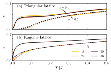
Figure 1: Comparison of FTLM results for the entropy $s(T)$, as obtained for different sizes $N=18-36$ for two characteristic $\alpha=0.1,0.5$ (a) for the triangular lattice, and (b) for the kagome lattice.

First, we consider the $h=0$ case. The central quantity evaluated within FTLM for a given system is the grand-canonical sum $Z(T)=\textrm{Tr}\{\exp[-(H-E_{0})]/T\}$ where $E_{0}$ is the gs energy. Orthogonalized FTLM reproduces exactly $Z(T\to 0)=1$ (for non-degenerate gs) even for $N_{s}=1$. Within the same procedure, we evaluate the entropy density

$$s(T)=[\ln Z+(\langle H\rangle-E_{0})/T]/N,$$ (2)

as well as the corresponding specific heat $c(T)=T(ds/dT)$ and the uniform (easy-axis) magnetic susceptibility $\chi_{0}={\cal M}^{2}/T$ (using theoretical units $k_{B}=g=\mu_{h}=1$) where the magnetization fluctuations are ${\cal M}^{2}=\langle(S^{z})^{2}\rangle/N$. Of special interest, in particular in relation to the QSL phenomenon, is the generalized Wilson ratio [35, 36, 34, 37]

$$R=4\pi^{2}T\chi_{0}/(3s),$$ (3)

which equals the standard Wilson ratio (constant at $T\to 0$) in the case of Fermi-liquid behavior at low $T$, i.e., for $s=c=\gamma T$. It should be noted that a constant $R(T\to 0)=R_{0}$ appears also within the Ising limit ($\alpha=0$) since $\chi_{0}\sim C/T$ and $s_{0}>0$, so that $R_{0}=4\pi^{2}C/(3s_{0})>0$. For the considered models at $\alpha>0$, this is not the case. Still we have $R(T)\propto{\cal M}^{2}(T)/s(T)$ at $T>0$ which represents a measure for the ratio of easy-axis magnetic excitations (contained in ${\cal M}^{2}$) to all excitations (represented with $s$). In particular, in the frustrated isotropic models, the signature of QSL is $R_{0}\to 0$ [36, 34], which is the case for $\alpha=1$ model on KL, but not on TL, where the lowest magnetic excitation is a triplet leading to a diverging $R_{0}\to\infty$.

It is relevant to realize the limitations of obtained numerical results for $T>0$. With the use of orthogonalized FTLM, statistical fluctuations at fixed $N$ are suppressed even at $T\to 0$, so the actual limitations are finite-size effects. For thermodynamic quantities, it is essential to capture enough many-body states. This requires $T>T_{fs}(N)$ [35] mostly reducing to an entropy requirement $s(T)>s_{min}(N)$. For the largest TL cluster with $N=36$, we estimate $s_{min}\sim 0.07$. In frustrated systems, this restriction comes into play only at very low $T\ll J$, in particular for at $\alpha\ll 1$, reflected in the quite accurate reproduction of the remanent gs entropy $s_{0}$. Conversely, long-range correlations remain more sensitive to $N$ as revealed in $S_{{\bf q}_{0}}(T\to 0)$.

To elucidate finite-size effects on thermodynamic quantities, we present a direct comparison of the results for entropy $s(T)$ on various $N=18-36$ and two different $\alpha=0.1,0.5$ in Fig. 1, both for TL and KL. Deviations are generally very small, with some finite-size discrepancies (related also to different lattice shapes) even in the limit $\alpha\to 0$ where exact result for TL is known to be $s_{0}=0.323$ [15, 26], while our finite-size result mildly deviate, e.g., in Fig. 4a we show $s_{0}=0.345$ (and corresponding $R_{0}$) obtained on $N=36$. A few conclusions directly follow: (a) finite-size effects on thermodynamic quantities are more pronounced for larger $\alpha\gtrsim 0.5$, both for TL and KL, which can be understood in terms of larger and $N$-dependent gaps, (b) finite-size effects are more visible for TL (also persisting to higher $T$), while being very small for KL. This has been realized already for the isotropic $\alpha=1$ case [34], (c) within TL and at $\alpha\ll 1$ our $T\to 0$ results can slightly deviate from exact $s_{0}=0.323$ (we get, e.g., for $N=36$ the value $s_{0}=0.345$ as shown in Fig. 4a) depending on actual lattices which are of different shapes, but all with PBC. On the other hand, such deviations are apparently quite negligible within KL as the finite systems reproduce the known exact $s_{0}=0.502$.

III Triangular lattice

III.1 Spin structure factor

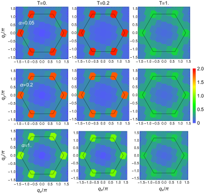
Figure 2: Color plots of the static spin structure factor $S_{\bf q}(T)$, as obtained via FTLM for anisotropic HM on TL with $N=30$ sites, shown for different $\alpha=0.05,0.2,1.0$ and $T=0,0.2,1$.

The spin structure factor $S_{\bf q}=(1/N)\sum_{i,j}\exp[i{\bf q}\cdot({\bf r}_{i}-{\bf r}_{j})]S^{z}_{i}S^{z}_{j}$ is expected to reveal the persistence of gs long-range spin correlations [20, 21, 22, 23, 24, 25] in the whole $\alpha\leq 1$ regime. Besides $T=0$ gs properties the behavior of $S_{\bf q}(T>0)$ is much less explored, except for the isotropic model [46]. Here, we present results for the $S_{\bf q}(T)$ within the anisotropic HM on TL, as obtained within FTLM on $N=30$ sites. In Fig. 2 we present numerical results for $S_{\bf q}(T)$ throughout the Brillouin zone (BZ) for ${\bf q}$ consistent with the finite-size $N=30$ lattice with PBC, for several $\alpha=0.05,0.2,1.0$ and different $T=0,0.1,0.5$. Apparently, the behavior at all considered $\alpha$ is qualitatively similar. At low $T$, the results reveal very pronounced maxima at the corners of the BZ ${\bf q}_{0}=(4\pi/3,0)$, being the signature of the LRO. It is significant that absolute and relative (to neighboring ${\bf q}\neq{\bf q}_{0}$, e.g., ${\bf q_{M}}$ at the middle BZ edge) maxima at ${\bf q}_{0}$ are even stronger in the Ising regime $\alpha\ll 1$. Clearly, at $T\sim 1$ the dependence on $\alpha$ is largely washed out.

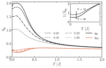
Figure 3: The spin structure factor $S_{\bf q}$ vs. $T$, calculated for the HM on TL with $N=30$ sites, presented for ${\bf q}={\bf q}_{0}$ at the BZ corner corresponding to ordering as well as for ${\bf q}={\bf q}_{M}$ in the middle of the BZ edge. The results correspond to various anisotropies, namely $\alpha=0.05,0.2,0.5,1$. The inset shows the comparison of $S^{-1}_{{\bf q}_{0}}(T)$ for $\alpha=0.05$ as calculated on $N=18,30$ sites, respectively.

More detailed results on $T$ dependence of $S_{\bf q}$ are shown in Fig. 3 for the ordering ${\bf q}={\bf q}_{0}$ and for more general ${\bf q}={\bf q}_{M}$ in the middle of the BZ edge. It should be noted that here we present results (for finite system $N=30$) in the whole range $T\geq 0$, although it is evident that results for $S_{\bf q}(T\sim 0)$ are size-dependent [23], due to long-range spin correlations, in particular for ${\bf q}={\bf q}_{0}$. This is confirmed by the comparison to our results on $N=18$, presented in the inset of Fig. 3 for $\alpha=0.05$ and ${\bf q}={\bf q}_{0}$. As expected $S_{{\bf q}_{0}}(T\sim 0)\propto\mu_{z}^{2}N$ is consistent with the gs LRO with the finite moment $\mu_{z}$. It is remarkable that the fall-off of $S_{{\bf q}_{0}}$ with $T$ is quite independent of $\alpha$ and does not appear to be related to the typical temperatures visible in thermodynamic quantities $s(T)$ and $\chi_{0}(T)$. On the other hand, as shown in Fig. 3 for other ${\bf q}={\bf q}_{M}$ inside the BZ, our results reveal some anomalies at low $T$ in the Ising regime, which seem to indicate the relation to $T^{*}\propto\alpha$ observed in, e.g., $s(T)$, although we cannot exclude that they disappear for increasing $N\to\infty$.

III.2 Thermodynamic quantities

We present results for the anisotropic HM on TL for various $\alpha$ between the Ising ($\alpha=0$) and the isotropic limit ($\alpha=1$) in Fig. 4: for the entropy density $s(T)$, inverse susceptibility $1/\chi_{0}(T)$ and the corresponding Wilson ratio $R(T)$ given by Eq. (3). All presented results in Fig. 4 are restricted to estimated $s>s_{min}$ since below they can be dominated by various finite-size effects. Results in Fig. 4(a) reproduce the residual entropy $s_{0}$ at $\alpha\to 0$ and $T\to 0$, whereas the effect of $\alpha>0$ is the final drop $s(T\ll T^{*})\to 0$, where $T^{*}\sim 0.3\alpha{J}$ is a characteristic crossover temperature. There is an evident high-$T$ regime, $T>T_{0}\sim 0.4\,{J}$, where $s(T)$, as well as other quantities, remain weakly dependent on $\alpha$.

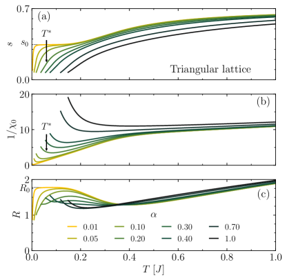
Figure 4: Entropy density $s(T)$ (a), inverse susceptibility $1/\chi_{0}(T)$ (b), and related Wilson ratio $R(T)$ (c) for the Heisenberg model, as obtained with FTLM on $N=36$ TL for anisotropies $0<\alpha\leq 1$. Thin dashed lines mark are the residual entropy $s_{0}$ in the Ising limit and the corresponding Wilson ratio $R_{0}$ while the arrows denote the crossover $T^{*}=0.3\alpha{J}$ for selected $\alpha=0.2$.

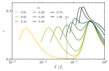
Figure 5: Specific heat $c$ vs. $T$ for the HM on TL for different $\alpha$. Marked is the maximum of the low-$T$ peak at $T^{*}=0.3\alpha{J}$ for $\alpha=0.2$.

The susceptibility $1/\chi_{0}(T)$ in Fig. 4(b) reveals several regimes. For $T>T_{0}$ the behavior (for all $\alpha$) follows the Curie-Weiss behavior with $\chi_{0}(T)\propto 1/(T+\Theta)$ where $\Theta\sim 1.5\,J$. On the other hand, in the Ising limit ($\alpha=0$), the dependence turns into a Curie law $\chi_{0}(T<T_{0})=C/T$ with $C=0.045$, where our value is comparable with $C=(5/36)/4=0.035$ from Ref. 16 and with $C=0.042$ from Ref. 18. In Appendix A we present an analytical analysis that gives a simple and quite accurate value of obtained Curie constant $C$.

The effect of finite $\alpha>0$ is the vanishing of $\chi_{0}(T\to 0)=0$, leading to pronounced maximum at $\chi_{0}(T\sim T^{*})$, i.e., the minimum of $\chi_{0}^{-1}(T\sim T^{*})$ in Fig. 4(b). The most important implication for the gs, however, follows from $R(T)$ shown in Fig. 4(c). The isotropic case of $\alpha=1$ has a minimum $R({T\sim 0.2\,J})$ [34] and $R(T\to 0)$ is expected to diverge (in the thermodynamic limit) due to the onset of magnetic LRO at $T=0$ (note that $T_{fs}>0.15\,J$ is the most restrictive for $\alpha\sim 1$). Results shown in Fig. 4(c) indicate that this minimum disappears for $\alpha<\alpha^{*}\sim 0.3$ and the behavior changes into the vanishing $R(T\to 0)=0$. Approaching $\alpha\to 0$ a broad plateau at the Ising value $R_{0}\sim 4\pi^{2}C/(3s_{0})$ also becomes evident and a downturn in $R(T)$ only occurs at $T<T^{*}$. Relevant for experiments is also the specific heat $c(T)$ presented in Fig. 5, directly related to $s(T)$ in Fig. 4(a). Its characteristic feature is a double-peak structure, becoming very pronounced for $\alpha\lesssim\alpha^{*}$. The high-$T$ peak at $T\sim 0.3\,{J}$ reflects correlations due to the dominant exchange $J$ and is nearly $\alpha$-independent. On the other hand, the maximum of the lower-energy peak coincides with the drop of $s(T)$ in Fig. 4(a) and occurs at $T\sim T^{*}$.

III.3 Lowest excitations

In order to understand the thermodynamic quantities, it is informative to follow the lowest excitations within the model. Their general structure within TL for $\alpha\leq 1$ is presented in Fig. 6. The gs (at $h=0$) belongs to the nonmagnetic $S^{z}=0$ sector. In the whole $\alpha<1$ range the lowest gap $\Delta_{0}$ belongs to a single nonmagnetic ($S^{z}=0$) state, lying below the first magnetic $S^{z}=1$ excitation with the gap $\Delta_{1}$. The next nonmagnetic gap is, however, $\Delta_{0}^{*}>\Delta_{1}$. The $N$ and $\alpha$ variations of gaps are very different in $\alpha\ll 1$ and $\alpha\sim 1$ regimes. In the latter, the magnetic $\Delta_{1}$ is expected to vanish with increasing $N$ as $\Delta_{1}\propto N^{-1}$, as established for $\alpha\sim 1$ [12]. This is consistent with our results in Fig. 6. We note that at least at $\alpha=1$, $\Delta_{0}$ should merge with $\Delta_{1}$, representing in this case the triplet excitation. On the other hand, the behavior for $\alpha<\alpha^{*}$ is markedly different. Results in Fig. 6 indicate that the magnetic $\Delta_{1}$ is almost $N$-independent and seems to converge to $\Delta_{1}\sim 0.5\alpha$. The lowest nonmagnetic $\Delta_{0}\ll\Delta_{1}$ that qualitatively explains the vanishing $R(T\to 0)\to 0$ in Fig. 4c, whereby $\Delta_{0}(N)$ might even vanish for $N\to\infty$. Still, higher nonmagnetic excitations are above the lowest magnetic one, i.e., $\Delta_{0}^{*}>\Delta_{1}$. This is in marked contrast with the analogous HM on KL, characterized by numerous nonmagnetic excitations below the lowest magnetic excitation in the whole regime of $\alpha\leq 1$, well established for $\alpha=1$ [39, 40, 34].

Figure 6: Magnetic and nonmagnetic gaps $\Delta_{1},\Delta_{0}$, respectively, vs. $\alpha$, as obtained on TL systems with $N=24-36$ sites. For $\alpha<0.5$ next-lowest-lying nonmagnetic excitations $\Delta^{*}_{0}$ are also presented. The dashed line in the lower panel shows the linear scaling of the magnetic gap on $\alpha$ in the Ising regime.

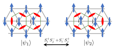
Figure 7: Configurations on TL in the gs manifold which allow a spin exchange without changing the Ising energy. Green hexagons show the dual honeycomb lattice [15, 26] with the red dimer indicating energetically unfavorable (parallel) orientation of spins on particular TL bond.

The emergence of the magnetic gap $\Delta_{1}$ at $\alpha>0$ can be considered through the lifting of the Ising gs degeneracy. For $\alpha\to 0$ one can apply the degenerate perturbation theory, in analogy to the Hubbard model for large $U$ [47], within which the concept of “interchangeable pairs” of spins emerged [19, 20], treating the $\alpha$ term perturbatively within the degenerate gs manifold. In our case, one transforms the Hamiltonian in such a way that it does not change the number of frustrated bonds. The application of the linear $\alpha$ term changes the configuration to the one shown on the right side of Fig. 7 (denoted with $|\psi_{2}\rangle$). The corresponding antisymmetric combination $|\psi_{s}\rangle=(|\psi_{1}\rangle-|\psi_{2}\rangle)/\sqrt{2}$ has lower energy $E_{s}=E_{0}-\alpha J/2$ ($E_{0}$ is the energy of the Ising gs manifold) and $S^{z}=0$. One can also create a $S^{z}=1$ state $|\psi_{t}\rangle=S^{+}_{i}|\psi_{1}\rangle$ by flipping the “free spin” on the site $i$ on the left configuration in Fig. 7 and making spins at sites $i$ and $j$ parallel. This state has $S^{z}=1$ and energy $E_{t}=E_{0}$ (up to a linear order in $\alpha$). Within this picture follows that $\Delta_{1}=E_{t}-E_{s}=\alpha J/2$, comparing favourably with FTLM results (see Fig. 6) for small $\alpha$.

III.4 Finite fields

The variation of the (normalized) magnetization density $m=\langle S^{z}\rangle/(NS)$ with external magnetic field $h$ in Eq. (1) can be evaluated within FTLM without additional numerical effort. The magnetization curves $m(h)$ are of particular interest also for the experiment since in related materials the whole regime of $h$ can potentially be explored. On frustrated lattices, such as TL and KL, a pronounced plateau at $m=1/3$ is expected and has been investigated within gs calculations [38]. The focus here is on the behavior at small finite $\alpha\ll 1$, since in the Ising limit ($\alpha=0$) the variation $m(h)$ is anomalous, with a discontinuous jump at $T\sim 0$, i.e., any small $h>0$ stabilizes the $m=1/3$ plateau. Numerical results for $m(h)$ for some characteristic $\alpha$ are presented in Fig. 8 where we show results up to $\alpha=1$ for completeness. The variation with $\alpha$ at small finite $T=0.1\,{J}$ reveals that the jump at $\alpha=0$ transforms into a nearly linear variation $m\propto h$ up to the $m=1/3$ plateau. At the same time, the plateau melts with increasing $T$ and essentially disappears for $T>T_{0}=0.4{J}$ even for small $\alpha$, as shown in Fig. 8(b).

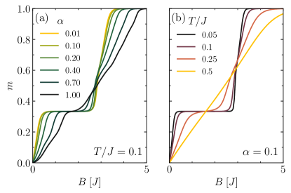
Figure 8: Magnetization curves $m(h)$ for the anisotropic HM on TL: (a) for different $\alpha$ at fixed $T=0.1$, and (b) for different $T$ at fixed $\alpha=0.1$.

IV Kagome lattice

IV.1 Spin structure factor

In contrast to TL, gs spin correlations within the anisotropic HM on KL are expected to be short-range even in the Ising limit $\alpha=0$ [26, 27]. Here, we present finite $T\geq 0$ results for easy-axis spin structure factor as obtained via FTLM for systems up to $N=30$ sites. We note that for isotropic $\alpha=1$ our $S_{\bf q}(T)$ results correspond well to previous studies [46]. In Fig. 9 we present results in analogy with Fig. 2, shown for the same $\bf q$ (taking the site/bond distance as unit $a=1$) as for TL (at same $N$). It is quite evident that (in contrast to TL) the variation of $S_{\bf q}(T)$ with ${\bf q}$ is quite smooth even in the gs with a weak maximum at the boundary of the extended BZ. The dependence on both $\alpha$ and $T$ is modest. This signals very short-range spin correlations and SL character, well established in the isotropic $\alpha=1$ case.

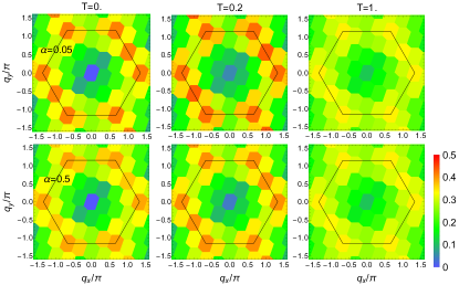
Figure 9: Color plots of the static spin structure factor $S_{\bf q}(T)$, as obtained via FTLM for anisotropic HM on KL with $N=30$ sites, shown for two $\alpha=0.05,0.5$ and $T=0.,0.2,1$.

IV.2 Thermodynamic quantities

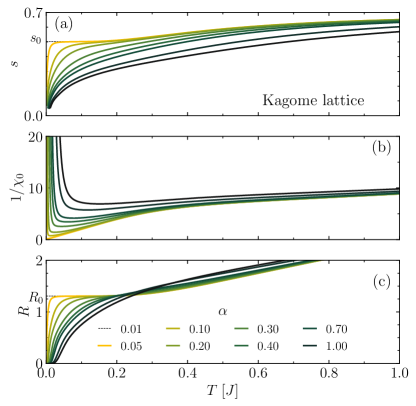
Figure 10: Thermodynamic quantities for the Heisenberg model on KL, as obtained with FTLM on $N=36$ sites for different $\alpha\leq 1$ : (a) entropy density $s(T)$, (b) inverse susceptibility $1/\chi_{0}(T)$, and (c) Wilson ratio $R(T)$. Marked are also exact $s_{0}=0.502$ as the Ising-limit result, and the corresponding Wilson ratio $R_{0}=1.306$.

We present further results for thermodynamic quantities for the anisotropic HM on KL, in analogy to previous results for TL. In Fig. 10 results are shown for various $\alpha\leq 1$ for entropy density $s(T)$, inverse susceptibility $1/\chi_{0}(T)$ and Wilson ratio $R(T)$, as obtained via FTLM on the largest KL with $N=36$ sites (the cutoff here is at $s>s_{min}=0.05$). In Fig. 11 the corresponding specific heat $c(T)$ is shown. The comparison with results on TL in Figs. 4,5 reveal similarities, but also pronounced qualitative differences between both lattices: (a) There is an essential difference close to the isotropic regime $\alpha\sim 1$, where HM on KL is the prominent example of a QSL without LRO [6, 7, 8, 9, 10], showing up also in the smoothly vanishing $R(T\to 0)$ [36, 34]. (b) In the regime $\alpha<\alpha^{*}$ for TL thermodynamic properties appear qualitatively similar. The drop of $s(T)$ from the Ising value $s_{0}$ with the corresponding lower peak in $c(T)$ appears at $T\sim T^{*}\sim 0.5\alpha\,{J}$. Related is the minimum of $1/\chi_{0}(T)$ in Fig. 10(b). (c) Still, there is a marked difference between TL and KL in the sharpness of the lower peak in $c(T)$. As evident in Fig. 11 the latter peak in KL extends to much lower $T$, which can be attributed to a large density of low-lying nonmagnetic excitations, valid also for the isotropic case HM at $\alpha=1$ [39, 40, 34]. Additional structure apparent in $c(T)$ at lowest $T\gtrsim T_{fs}$ can be partly attributed to finite-size effects, as also observed for $\alpha=1$ for even larger $N=42$ [10].

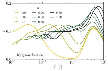
Figure 11: Specific heat $c$ vs. $T$ (in log scale) for the anisotropic HM on KL for various $\alpha$.

IV.3 Lowest excitations

In analogy to TL, we also analyze the gap structure on KL. In Fig. 12 we present the variation of the magnetic gap $\Delta_{1}$ with $\alpha$ for different system sizes $N$. The gap vanishes (linearly for all $N$) approaching Ising limit $\alpha\to 0$, in analogy to TL in Fig. 8. However, the gap for KL increases steadily up to $\alpha\lesssim 1$, which is in contrast to TL. The $N$ dependence is less systematic even at $\alpha\lesssim 1$ in accordance with the open question whether $\Delta_{1}$ remains finite in the $N\to\infty$ limit [39]. The same question applies to our results in Fig. 12 for the regime of $\alpha\ll 1$, where we do not observe clear convergence with $N$, unlike the TL case in Fig. 6. However, the crucial difference to TL is the behavior of nonmagnetic excitations. It is known that in the isotropic case, there are (macroscopically) numerous nonmagnetic excitations below the lowest magnetic one [39, 40]. Our results reveal that this remains the case in the whole regime of $\alpha\leq 1$, i.e., we find many $S^{z}=0$ states satisfying $\Delta_{0}\ll\Delta_{1}$, which are hard to enumerate fully within our Lanczos-based method.

Presented results for the HM on KL offer an important insight into the well-established QSL state in that its properties in the isotropic $\alpha=1$ model are smoothly connected to the Ising-like regime at $\alpha\ll 1$. This contrasts with the corresponding HM on TL.

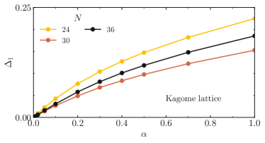
Figure 12: The magnetic gap $\Delta_{1}$ vs. $\alpha$, obtained on KL systems with $N=24-36$ sites.

IV.4 Finite fields

Finally, we show results for the magnetization curves $m(h)$ for KL. Again, in the Ising limit $\alpha=0$ the variation $m(h)$ reveals a discontinuous jump at $T\sim 0$, i.e., even small $h>0$ stabilizes $m=1/3$ magnetization. Numerical results for $m(h)$ for some characteristic cases are presented in Fig. 13. The variation with $\alpha$ at small finite $T=0.1\,{J}$ shows that the jump at $\alpha=0$ transforms into a nearly linear variation $m\propto h$ up to the $m=1/3$ plateau. At the same time, the plateau disappears with increasing $T>T_{0}$ already at small $\alpha\ll 1$, as shown in Fig. 13(b).

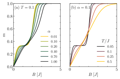
Figure 13: Magnetization curves $m(h)$ for the anisotropic HM on KL: (a) for different $\alpha$ at fixed $T=0.1$, and (b) for different $T$ at fixed $\alpha=0.1$.

V Discussion

Isotropic AFM spin models on frustrated lattices have been intensively studied, mostly as candidates for the QSL phenomenon. The anisotropy studied here offers another route to interesting collective phenomena. Our analysis indicates that with the increasing easy-axis anisotropy, the thermodynamic quantities within Heisenberg model on TL undergo a crossover from the isotropic-like regime to the Ising regime at $\alpha<\alpha^{*}\sim 0.3$, most pronounced in the behavior of the Wilson ratio $R(T\to 0)$ vanishing at $\alpha<\alpha^{*}$ and increasing for $\alpha>\alpha^{*}$, at least within the range of low $T$ but above finite-size $T>T_{fs}(N)$. On the other hand, spin correlations as displayed in $S_{\bf q}(T\to 0)$ are consistent with LRO in the gs in the whole $\alpha\leq 1$ regime, thus apparently coexisting with strongly $\alpha$-dependent thermodynamic properties. It is quite remarkable that the calculated thermodynamic quantities, at least in the Ising regime $\alpha\ll 1$, do not exhibit any significant finite-size effects down to the lowest $T<T_{fs}\ll\alpha J$ while the gs static spin structure factor $S_{{\bf q}_{0}}$ remains consistent with gs LRO and consequently also with finite-size ($N$) dependence $S_{{\bf q}_{0}}(T\to 0)\propto N$, but at the same time not reflecting any evident influence of the quantum-fluctuation scale $T^{*}\propto\alpha$.

Remarkably, in the Ising limit ($\alpha=0$), there are analogies between the low-$T$ thermodynamic properties of spin models on the TL and KL. In particular, the existence of remanent entropy $s_{0}>0$ and the Curie susceptibility $\chi_{0}\sim C/T$. However, in contrast to the TL case, in the KL case there is a continuous (smooth) variation of all quantities from $\alpha\gtrsim 0$ regime to the most studied isotropic $\alpha=1$ QSL. Moreover, on KL, contrary to TL, there are numerous nonmagnetic excitations below the lowest magnetic one (i.e., the triplet at $\alpha=1$ [39, 40, 34]) within the whole range of $\alpha\leq 1$. Still, there are evident differences in the spin correlations. In contrast to TL, within KL spin structure factor $S_{\bf q}(T)$ smoothly varies with ${\bf q}$ within the BZ, but only weakly depends on $T$ and $\alpha$, consistent with the short-range correlations and the QSL character.

Finally, let us return to the potential relevance of our study for experimental realizations of anisotropic HM on TL and KL. Recently, the TL antiferromagnet NdTa₇O₁₉ was shown to host dominant Ising spin correlations between nearest neighbors and the anisotropy was estimated to be $\alpha=0.18$ [33]. This estimate was based on the assumption that the exchange anisotropy in the lowest order follows the anisotropy of the $g$ factor squared [48]. Various experiments suggest QSL gs arising from strong Ising anisotropy of the exchange interactions. A direct comparison to our results is at present limited, as susceptibility data are so far restricted to powder samples at $T\gtrsim J$, and the specific heat has not been measured yet. Recently, the delafossite compound KTmSe₂ has been also proposed as another quantum-Ising TL candidate [49].

Appendix A Origin of the Curie susceptibility

Figure 14: Probability of states with given $S^{z}$ in the Ising gs manifold, relative to the total number of states. The distribution is numerically calculated for TL and for KL on $N=36$ sites and fitted with the Gaussian (dashed lines). Note that the normalized probabilities are small due to a large portion of non-free spins in the system.

In the Ising limit $\alpha=0$ the Curie susceptibility is related to “free spins” or “orphans” [15, 31, 26], which can be flipped without any energy cost within the gs manifold. From the magnetization curves in Fig. 8(a) and gs results showing $m=1/3$ plateau one can estimate the density of free spins as $p_{\textrm{free}}=1/6$, based on the observation that any $h\gtrsim 0$ at $T=0$ leads to $m=1/3$. The resulting $C=p_{\textrm{free}}/4=0.042$ compares well with FTLM numerical results of $C=0.045$, as obtained from Fig. 4(b). Further support for this interpretation can be made by counting the number of states with a certain total $S^{z}$, within the gs manifold. Such distribution is a Gaussian and our numerical results comply well with that (see Fig. 14). The width of the distribution is directly related to the number of free spins and by fitting it we get $p_{\textrm{free}}=0.176$, leading to the estimate $C=0.044$, which agrees even better with the FTLM result.

The Ising limit ($\alpha=0$) has a macroscopically degenerate gs. In such a case, the spin susceptibility can be written as

$$\chi_{0}=\frac{1}{NT}\sum_{S^{z}}p_{S^{z}}(S^{z})^{2},$$ (4)

where $p_{S^{z}}=N_{S^{z}}/N_{all}$ with $N_{S^{z}}$ is the number of many-body states with some value of $S^{z}$ and $N_{all}$ is the total number of all states in the gs manifold. Assuming $N_{f}$ free spins, each state can have a certain number of up spins $N_{\uparrow}$ and down spins $N_{\downarrow}$ so that $N_{f}=N_{\uparrow}+N_{\downarrow}$. Further one can write the probability for $S^{z}=\frac{1}{2}(N_{\uparrow}-N_{\downarrow})=N_{\uparrow}-\frac{1}{2}N_{f}$ as

$$p_{S^{z}}=\frac{1}{2^{N_{f}}}\binom{N_{f}}{N_{\uparrow}}\approx\sqrt{\frac{2}{\pi N_{f}}}\textrm{e}^{-2(S^{z})^{2}/N_{f}}\leavevmode\nobreak\$$ (5)

by using the normal approximation for large $N_{f}$ and $N_{\uparrow}$. The probability of free spins becomes Gaussian for large systems and we clearly observe such behavior numerically on $N=36$ sites within an Ising gs manifold by counting the number of states (see Fig. 14). Further, the fitted width of the Gaussian is an estimate of the number of free spins $N_{f}$, which gives a good estimate for the Curie constant $C=N_{f}/(4N)=0.044$ for TL and $C=0.051$ for KL.

References

- Anderson [1973] P. W. Anderson, Mat. Res. Bull. 8, 153 (1973).
- Mila [2000] F. Mila, Eur. J. Phys. 21, 499 (2000).
- Lee [2008] P. A. Lee, Science 321, 1306 (2008).
- Balents [2010] L. Balents, Nature 464, 199 (2010).
- Savary and Balents [2017] L. Savary and L. Balents, Rep. Prog. Phys. 80, 016502 (2017).
- Mila [1998] F. Mila, Phys. Rev. Lett. 81, 2356 (1998).
- Budnik and Auerbach [2004] R. Budnik and A. Auerbach, Phys. Rev. Lett. 93, 187205 (2004).
- Läuchli et al. [2011] A. M. Läuchli, J. Sudan, and E. S. Sørensen, Phys. Rev. B 83, 212401 (2011).
- Iqbal et al. [2013] Y. Iqbal, F. Becca, S. Sorella, and D. Poilblanc, Phys. Rev. B 87, 060405(R) (2013).
- Schnack et al. [2018] J. Schnack, J. Schulenburg, and J. Richter, Phys. Rev. B 98, 094423 (2018).
- Bernu et al. [1994] B. Bernu, P. Lecheminant, C. Lhuillier, and L. Pierre, Phys. Rev. B 50, 10048 (1994).
- Capriotti et al. [1999] L. Capriotti, A. E. Trumper, and S. Sorella, Phys. Rev. Lett. 82, 3899 (1999).
- White and Chernyshev [2007] S. R. White and A. L. Chernyshev, Phys. Rev. Lett. 99, 127004 (2007).
- Chernyshev and Zhitomirsky [2009] A. L. Chernyshev and M. E. Zhitomirsky, Phys. Rev. B 79, 144416 (2009).
- Wannier [1950] G. H. Wannier, Phys. Rev. 79, 357 (1950).
- Sykes and Zucker [1961] M. Sykes and I. J. Zucker, Phys. Rev. 52, 410 (1961).
- Miyashita and Kawamura [1985] S. Miyashita and H. Kawamura, J. Phys. Soc. Jpn. 54, 3385 (1985).
- Sano [1987] K. Sano, Prog. Theor. Phys. 77, 287 (1987).
- Fazekas and Anderson [1974] P. Fazekas and P. W. Anderson, Philos. Mag. 30, 423 (1974).
- Kleine et al. [1992a] B. Kleine, P. Fazekas, and E. Müller-Hartmann, Z. Phys. B 86, 405 (1992a).
- Kleine et al. [1992b] B. Kleine, E. Müller-Hartmann, F. K., and P. Fazekas, Z. Phys. B 87, 103 (1992b).
- Wang et al. [2009] F. Wang, F. Pollmann, and A. Vishwanath, Phys. Rev. Lett. 102, 017203 (2009).
- Jiang et al. [2009] H. C. Jiang, M. Q. Weng, Z. Y. Weng, D. N. Sheng, and L. Balents, Phys. Rev. B 79, 020409 (2009).
- Yamamoto et al. [2014] D. Yamamoto, G. Marmorini, and I. Danshita, Phys. Rev. Lett. 112, 127203 (2014).
- Sellmann et al. [2015] D. Sellmann, X.-F. Zhang, and S. Eggert, Phys. Rev. B 91, 081104 (2015).
- Moessner et al. [2000] R. Moessner, S. L. Sondhi, and P. Chandra, Phys. Rev. Lett. 84, 4457 (2000).
- Moessner and Sondhi [2001] R. Moessner and S. L. Sondhi, Phys. Rev. B 63, 224401 (2001).
- Mostovoy et al. [2003] M. V. Mostovoy, D. I. Khomskii, J. Knoester, and N. V. Prokof’ev, Phys. Rev. Lett. 90, 4 (2003).
- Chern and Tsukamoto [2008] C. H. Chern and M. Tsukamoto, Phys. Rev. B 77, 4 (2008).
- Chen [2019] G. Chen, Phys. Rev. Res. 1, 033141 (2019).
- Isoda [2008] M. Isoda, J. Phys. Condens. Matter 20, 315202 (2008).
- Isoda et al. [2011] M. Isoda, H. Nakano, and T. Sakai, J. Phys. Soc. Jpn. 80, 1 (2011).
- Arh et al. [2022] T. Arh, B. Sana, M. Pregelj, P. Khuntia, Z. Jagličić, M. D. Le, P. K. Biswas, P. Manuel, L. Mangin-Thro, A. Ozarowski, and A. Zorko, Nat. Mater. 21, 416 (2022).
- Prelovšek et al. [2020] P. Prelovšek, K. Morita, T. Tohyama, and J. Herbrych, Phys. Rev. Res. 2, 1 (2020).
- Jaklič and Prelovšek [2000] J. Jaklič and P. Prelovšek, Adv. Phys. 49, 1 (2000).
- Prelovšek and Kokalj [2018] P. Prelovšek and J. Kokalj, Phys. Rev. B 98, 035107 (2018).
- Richter et al. [2022] J. Richter, O. Derzhko, and J. Schnack, Phys. Rev. B 105, 144427 (2022).
- Honecker et al. [2004] A. Honecker, J. Schulenburg, and J. Richter, J. Phys. Condens. Matter 16, 10.1088/0953-8984/16/11/025 (2004).
- Waldtmann et al. [1998] C. Waldtmann, H. U. Everts, B. Bernu, C. Lhuillier, P. Sindzingre, P. Lecheminant, and L. Pierre, Eur. Phys. J. B 2, 501 (1998).
- Läuchli et al. [2019] A. M. Läuchli, J. Sudan, and R. Moessner, Phys. Rev. B 100, 155142 (2019).
- Jaklič and Prelovšek [1994] J. Jaklič and P. Prelovšek, Phys. Rev. B 49, 5065 (1994).
- Prelovšek and Bonča [2013] P. Prelovšek and J. Bonča, in Strongly Correlated Systems - Numerical Methods, edited by A. Avella and F. Mancini (Springer, Berlin, 2013).
- Prelovšek et al. [2021] P. Prelovšek, M. Gomilšek, T. Arh, and A. Zorko, Phys. Rev. B 103, 014431 (2021).
- Wietek and Läuchli [2018] A. Wietek and A. M. Läuchli, Phys. Rev. E 98, 033309 (2018).
- Morita [2022] K. Morita, Phys. Rev. B 105, 064428 (2022).
- Morita and Tohyama [2020] K. Morita and T. Tohyama, Phys. Rev. Res. 2, 013205 (2020).
- Eskes et al. [1994] H. Eskes, A. M. Oleś, M. B. J. Meinders, and W. Stephan, Phys. Rev. B 50, 17980 (1994).
- Abragam and Bleaney [1970] A. Abragam and B. Bleaney, Electron Paramagnetic Resonance of Transition Ions (Clarendon Press, 1970).
- Zheng et al. [2023] S. Zheng, H. Wo, Y. Gu, R. L. Luo, Y. Gu, Y. Zhu, P. Steffens, M. Boehm, Q. Wang, G. Chen, and J. Zhao, arXiv:2305.19824 10.48550/arXiv.2306.03544 (2023).