Randomized subspace gradient method for constrained optimization

Abstract

We propose randomized subspace gradient methods for high-dimensional constrained optimization. While there have been similarly purposed studies on unconstrained optimization problems, there have been few on constrained optimization problems due to the difficulty of handling constraints. Our algorithms project gradient vectors onto a subspace that is a random projection of the subspace spanned by the gradients of active constraints. We determine the worst-case iteration complexity under linear and nonlinear settings and theoretically confirm that our algorithms can take a larger step size than their deterministic version. From the advantages of taking longer step and randomized subspace gradients, we show that our algorithms are especially efficient in view of time complexity when gradients cannot be obtained easily. Numerical experiments show that they tend to find better solutions because of the randomness of their subspace selection. Furthermore, they performs well in cases where gradients could not be obtained directly, and instead, gradients are obtained using directional derivatives.

1 Introduction

In this paper, we consider the following constrained optimization problem:

$${}\begin{split}&\min_{x\in\mathbb{R}^{n}}f(x)\\ &\mathrm{s.t.}\;\mathcal{C}:=\{x~{}|~{}g_{i}(x)\leq 0,\quad i=1,...,m\},\end{split}$$ (1)

where $f$ is $L$-smooth and $g_{i}$ are $L_{g}$-smooth, neither of which need be convex functions as long as an optimal solution exists. There is a growing demand for solving large-scale constrained optimization problems in many applications such as machine learning, statistics, and signal processing tibshirani2005sparsity ; lee1999learning ; zafar2017fairness ; komiyama2018icml ; moldovan2012safe ; achiam2017constrained ; for example, sparse optimization problems are often formulated as

$$\min_{x}L(x)\;\mathrm{s.t.}\;\mathcal{R}(x)\leq s,$$ (2)

where $L(x)$ is a loss function, $\mathcal{R}$ is some sparsity-inducing norm such as $l_{1}$, and $s$ is some fixed positive integer value. Recently, machine-learning models (2) including a fairness constraint zafar2017fairness ; komiyama2018icml have attracted researchers’ attention, but difficulties have emerged in solving such large-scale problems.

For solving large-scale unconstrained problems, i.e., (2) with $\mathcal{C}=\mathbb{R}^{n}$, kozak2021stochastic ; gower2019rsn ; hanzely2020stochastic ; fuji2022randomized ; chen2020randomized ; berglund2022zeroth ; cartis2022randomised have proposed subspace methods using random projection. These methods update the iterate point as follows:

$${}x_{k+1}=x_{k}+M_{k}d_{k},$$ (3)

where $M_{k}$ is an $n\times d$ ($d<n$) random matrix. One of the difficulties with high-dimensional problems is calculating the gradient $\nabla f$. Although there are some methods that calculate gradients, such as automatic differentiation that is popular in machine learning, when the objective function has a complicated structure, backward-mode automatic differentiation leads to an explosion in memory usage margossian2019review . Kozak et al. kozak2021stochastic proposed a stochastic subspace descent method combining gradient descent with random projections to overcome the difficulties of calculating gradients. The method uses the direction $d_{k}=-M_{k}^{\top}\nabla f(x_{k})$, and it was shown that $d_{k}$ can be computed by using finite-difference or forward-mode automatic differentiation of the directional derivative. To obtain the full gradients by using finite difference or forward-mode automatic differentiation, we need to evaluate the function values $n$ times. On the other hand, the projected gradient can be computed by evaluating the function values only $d$ times.

Compared with unconstrained problems, subspace optimization algorithms using random projections have made little progress in solving constrained problems. To the best of our knowledge, apart from cartis2022bound , there is no paper on subspace optimization algorithms using (3) for constrained optimization (1). Here, Cartis et al. cartis2022bound proposed a general framework to investigate a general random embedding framework for bound-constrained global optimization of $f$ with low effective dimensionality. The framework projects the original problem onto a random subspace and solves the reduced subproblem in each iteration:

$$\min_{d}f(x_{k}+M_{k}d)~{}~{}\mbox{subject to}~{}x_{k}+M_{k}d\in\mathcal{C}.$$

These subproblems need to be solved to some required accuracy by using a deterministic global optimization algorithm.

In this study, we propose gradient-based subspace methods for constrained optimization. The descent direction $d_{k}$ is obtained without solving any subproblems, by projecting the gradient vector $\nabla f$ onto a subspace that is a random projection of the subspace spanned by the gradients of the active constraints. A novel property of our algorithms is that when the dimension $n$ is large enough, they are almost unaffected by the constraint boundary; because of this, they can take a longer step than their deterministic versions. In standard constrained optimization methods, the iterates become difficult to move when they get close to the constraint boundary. Our methods randomly update the subspace where the iterate is reconstructed in each iteration, which makes it possible for them to take a large step.

We present two randomized subspace gradient algorithms: one is specialized for linear constrained optimization problems and the other is able to handle nonlinear constraints. On linearly constrained problems, these algorithms work very similarly to the gradient projection method rosen1960gradient if random projections are not used. The gradient projection method (GPM) rosen1960gradient ; du1990rosen is one of the active set methods. Under linear constraints, GPM projects the gradients $\nabla f$ onto a subspace spanned by the gradients of the active constraints. The projected gradient does not change the function values of active constraints. Hence, the advantage of GPM is that all of the updated points are feasible. Rosen rosen1961gradient augmented GPM to make it able to handle nonlinear constraints and proved global convergence. Also for nonlinear constraints, a generalized gradient projection method (GGPM) gao1996generalized ; wang2013generalized was derived from GPM; it does not require an initial feasible point.

Our algorithms need $O(\frac{n}{d}\varepsilon^{-2})$ iterations to reach an approximate Karush-Kuhn-Tucker (KKT), while other standard gradient-algorithms for solving unconstrained problems need $O(\varepsilon^{-2})$ iterations. While the theoretical worst-case iteration complexity increases because of the subspace projection, the gradient computation at each iteration costs less; when gradients cannot be obtained easily, our algorithms have the same advantage as stochastic subspace gradients kozak2021stochastic by calculating the gradients with $d$ directional derivatives. Due to their advantages of taking longer step and reducing the computational complexity of calculating the gradients, our algorithms are especially efficient in view of time complexity. This is because when gradients are obtained by directional derivatives, ours need $O(d)\times O(\frac{n}{d}\varepsilon^{-2})$ function evaluations to reach an approximate KKT, which is the same as the number of evaluations in standard gradient-algorithms for solving unconstrained problems ($O(n)\times O(\varepsilon^{-2})$). Furthermore, our algorithms can reduce the worst time complexity to reach an approximate KKT from $O(n)\times O(\max{(\varepsilon^{-2},(u_{g}^{\varepsilon})^{-1}\varepsilon^{-2})})$ to $O(d)\times O(\frac{n}{d}\varepsilon^{-2})$ compared to their deterministic version when gradients are obtained by directional derivatives. $u_{g}^{\varepsilon}$ represents a particular value that is dependent on the given constraints and the parameter $\varepsilon$. In the case where all constraints are linear functions, $u_{g}^{\varepsilon}$ simplifies to $\varepsilon$.

In numerical experiments, we show that our algorithms work well when the gradient of the objective functions cannot be calculated. The numerical results indicate that our algorithms tend to find better solutions than deterministic algorithms, because they can search for solutions randomly in a wide space without being affected by the luck involved in the initial solution selection.

2 Preliminaries

2.1 Notations

In this paper, we denote the optimum of (1) by $x^{*}$. The vector norm $\|\cdot\|$ is assumed to be the $l_{2}$ norm and the matrix norm is the operator norm. $\|\cdot\|_{F}$ denotes the Frobenius norm. $\lambda_{\mathrm{min}}(A)$ and $\lambda_{\mathrm{max}}(A)$ are the minimum eigenvalue and maximum eigenvalue of a matrix $A$, respectively.

For a vector $a$, we define $[a]_{+}$ be a vector whose $i$-th entry is given by $[a_{i}]_{+}:=\max(0,a_{i})$. $\bm{1}$ denotes an all-ones vector and $\chi_{S}(x)$ denotes a step function for all $x\in\mathbb{R}$;

$$\chi_{S}(x)=\left\{\begin{array}[]{cc}1&(x\in S),\\ 0&(x\notin S).\\ \end{array}\right.$$

$\chi_{-}$ and $\chi_{+}$ are step functions with $S=\{x|x\leq 0\}$ and $S=\{x|x>0\}$, respectively. For a vector $a$, we define $\chi_{+}(a)$ (or $\chi_{-}(a)$) to be a vector whose $i$-th entry is $\chi_{+}(a_{i})$ (or $\chi_{-}(a_{i})$, respectively).

2.2 Key lemma

The following lemma implies that a random projection defined by a random matrix $P$ nearly preserves the norm of any given vector $x$ with arbitrarily high probability. It is a variant of the Johnson-Linderstrauss lemma jllemma .

Lemma 1.

vershynin2018high Let $P\in\mathbb{R}^{d\times n}$ be a random matrix whose entries are independently drawn from $\mathcal{N}(0,1)$. Then for any $x\in\mathbb{R}^{n}$ and $\varepsilon\in(0,1)$, we have

$$\mathrm{Prob}[(1-\varepsilon)\|x\|^{2}\leq\frac{1}{d}\|Px\|^{2}\leq(1+\varepsilon)\|x\|^{2}]\geq 1-2\exp{(-C_{0}\varepsilon^{2}d)},$$

whose $C_{0}$ is an absolute constant.

3 Algorithm for linear inequality constraints

In this section, we describe our randomized subspace gradient method for solving linear constrained problems (RSG-LC), which is listed as Algorithm 1 below.

Algorithm 1 Randomized Subspace Gradient Method for Linear Constrained Problems (RSG-LC)

INPUT: $x_{0}$ (a feasible point), step size $h>0$, reduced dimension $d$, $\varepsilon_{0},\delta_{1},\varepsilon_{2}>0,1>\beta>0$.

for $k=0,1,2,...$ do

     $\alpha_{k}=h$

     Set $M_{k}=\frac{1}{n}P_{k}^{\top}$ by sampling a random matrix $P_{k}\in\mathbb{R}^{d\times n}\sim\mathcal{N}$.

     Set $G_{k}=\left(\nabla g_{i}(x_{k})\right)_{i\in\mathcal{A}_{k}}\in\mathbb{R}^{n\times|\mathcal{A}_{k}|}$ by using $\mathcal{A}_{k}$ defined in (7).

     Compute

$$\lambda^{(k)}=-(G_{k}^{\top}M_{k}M_{k}^{\top}G_{k})^{-1}G_{k}^{\top}M_{k}M_{k}^{\top}\nabla f(x_{k})$$ (4)

and

$$d_{k}=-M_{k}^{\top}\left(\nabla f(x_{k})+G_{k}\lambda^{(k)}\right).$$ (5)

     if $\|d_{k}\|\leq\delta_{1}$ then

         if $\min_{i}\lambda^{(k)}_{i}\geq-\varepsilon_{2}$ then

              terminate.

         else

              

$$d_{k}=-\frac{d}{n}M_{k}^{\top}G_{k}(G_{k}^{\top}M_{k}M_{k}^{\top}G_{k})^{-1}\left[-\lambda^{(k)}\right]_{+}$$ (6)

         end if

     end if

     while $x_{k}+\alpha_{k}M_{k}d_{k}$ is not feasible do

         $\alpha_{k}\leftarrow\beta\alpha_{k}$

     end while

     $x_{k+1}\leftarrow x_{k}+\alpha_{k}M_{k}d_{k}$

end for

3.1 Outline of our algorithm: RSG-LC

Let $\mathcal{N}$ denote the set of Gaussian matrices of size $d\times n$ whose entries are independently sampled from $\mathcal{N}(0,1)$, and define $M_{k}=\frac{1}{n}P_{k}^{\top}$, where $P_{k}$ is a Gaussian random matrix sampled from $\mathcal{N}$.

Definition of $\mathcal{A}_{k}$

Let $\mathcal{A}_{k}:=\mathcal{A}(x_{k})$ be the index set of active constraints such that the inequality constraints are almost satisfied by equality at the iterate $x_{k}$. The active set usually refers to the set of indices whose constraints satisfy $g_{i}(x)=0$. We use loose criteria for the active set of our randomized subspace algorithm:

$$\mathcal{A}(x)=\left\{i\in\{1,2,\cdots,m\}|\ [-g_{i}(x)]_{+}\leq\varepsilon_{0}\|\nabla g_{i}(x)\|\right\}$$ (7)

using a parameter $\varepsilon_{0}$ $(>0)$.

Section 3.3 shows that the definition of $\mathcal{A}_{k}$ makes the iterates $\{x_{k}\}$ all feasible with high probability, and that the step size $\alpha_{k}$ is larger than when the random matrices are not used. Notice that we can replace $\nabla g_{i}$ in $\mathcal{A}_{k}$ with the projected gradients $M_{k}^{\top}\nabla g_{i}$ to reduce the computation costs when calculating $\nabla g_{i}$ is difficult. This is because, from Lemma 1, $\frac{[-g_{i}(x_{k})]_{+}}{\|M_{k}^{\top}\nabla g_{i}(x_{k})\|}\approx\frac{n}{\sqrt{d}}\frac{[-g_{i}(x_{k})]_{+}}{\|\nabla g_{i}(x_{k})\|}$ holds with high probability. Therefore, the active set $\mathcal{A}_{k}$ using projected gradients can be almost the same as the set using the full gradients by adjusting $\varepsilon_{0}$. For the sake of simplicity, we define $\frac{[-g_{i}(x_{k})]_{+}}{\|\nabla g_{i}(x_{k})\|}\leq\varepsilon_{0}$ to be the active set $\mathcal{A}_{k}$.

Update of Iterates

Algorithm 1 calculates the sequence $\{x_{k}\}$ by using the step size $\alpha_{k}$ and the Lagrange multiplier $\lambda^{(k)}\in\mathbb{R}^{|\mathcal{A}_{k}|}$ of (4) corresponding to constraints in $\mathcal{A}_{k}$ as

$$x_{k+1} =x_{k}-\alpha_{k}M_{k}M_{k}^{\top}\left(\nabla f(x_{k})+G_{k}\lambda^{(k)}\right)$$ (8)

$$=x_{k}-\alpha_{k}M_{k}\left(I-M_{k}^{\top}G_{k}(G_{k}^{\top}M_{k}M_{k}^{\top}G_{k})^{-1}G_{k}^{\top}M_{k}\right)M_{k}^{\top}\nabla f(x_{k})$$

or

$$x_{k+1}=x_{k}-\frac{d}{n}\alpha_{k}M_{k}M_{k}^{\top}G_{k}(G_{k}^{\top}M_{k}M_{k}^{\top}G_{k})^{-1}\left[-\lambda^{(k)}\right]_{+},$$ (9)

where $G_{k}=\left(\nabla g_{i}(x_{k})\right)_{i\in\mathcal{A}_{k}}\in\mathbb{R}^{n\times|\mathcal{A}_{k}|}$. This corresponds to taking $d_{k}$ as (5) or (6).

The search directions $x_{k+1}-x_{k}$ in (8) and (9) are descent directions with high probability as shown in Propositions 1 and 2 in Section 3.2. Propositions 3 and 4 in Section 3.3 ensure that if the $\alpha_{k}$ are chosen to be less than some threshold, all points in $\{x_{k}\}$ are feasible. Hence, the while-loop reducing the value of $\alpha_{k}$ stops after a fixed number of iterations. Theoretically, (8) reduces the objective function more than (9) does at each iteration. Therefore, the algorithm first computes (8) and if the search direction is small enough and the Lagrange multiplier $\lambda^{(k)}$ is not nonnegative, (9) is used for the next iterate $x_{k+1}$.

The search direction in (8) is regarded as the projected gradient vector onto a subspace that itself is a random projection of the subspace spanned by the gradients of active constraints. Note that if we ignore the random matrix $M_{k}$ (i.e., by setting $M_{k}=I$), the update rule of (8) becomes

$$x_{k+1}=x_{k}-\alpha_{k}\left(I-G_{k}(G_{k}^{\top}G_{k})^{-1}G_{k}^{\top}\right)\nabla f(x_{k})$$

and $\left(I-G_{k}(G_{k}^{\top}G_{k})^{-1}G_{k}^{\top}\right)\nabla f(x_{k})$ is the projected gradient onto the subspace spanned by the gradients of the active constraints in $\mathcal{A}_{k}$. If $\mathcal{A}_{k}$ is an active set in the usual sense defined by the valid constraints, the projected gradient is the same as the one used in the gradient projection method (GPM) rosen1960gradient .

By the definition of $d_{k}$ of (5), if $\|d_{k}\|\approx 0$, then $\|\nabla f(x_{k})+G_{k}\lambda^{(k)}\|\approx 0$ holds by Lemma 1. If $\lambda^{(k)}\geq 0$ holds, the resulting point is an approximate Karush-Kuhn-Tucker (KKT) point. As shown later in Theorem 5, given inputs $d,\varepsilon_{0},\varepsilon_{2}$ and $\delta_{1}=\sqrt{\frac{d(1-\varepsilon)}{n^{2}}}\varepsilon_{1}$, Algorithm 1 generates for the original problem (1) with large $n$ an output $x_{k}$ that is with high probability an $(\varepsilon_{1},\varepsilon_{2},O(\varepsilon_{0}))$-KKT point within $O(\frac{n}{d\min(\varepsilon_{1}^{2},\varepsilon_{2}^{2})})$ iterations.

3.2 Decrease in objective value

We will make the following assumptions.

Assumption 1.

1. $f$ is $L$-smooth, i.e., $\|\nabla f(x)-\nabla f(y)\|\leq L\|x-y\|$ for any $x,y\in\mathbb{R}^{n}$.

2. The level set $\{x\in\mathcal{C}|f(x)\leq f(x_{0})\}$ is compact.

(i) and (ii) together imply that $\|\nabla f(x_{k})\|$ is bounded, i.e., $\|\nabla f(x_{k})\|\leq U_{f}$ for some value $U_{f}>0$.

Assumption 2.

1. The vectors $\nabla g_{i}(x)$, $\forall i\in\mathcal{A}_{k}$, of the active constraints at $x_{k}\in\mathcal{C}$ are linearly independent.

2. The reduced dimension $d$ is larger than the number of active constraints $|\mathcal{A}_{k}|$.

Notice that Assumption 2 implies that $M_{k}^{\top}G_{k}$ has full row rank with probability 1, which ensures the existence of $(G_{k}^{\top}M_{k}M_{k}^{\top}G_{k})^{-1}$. Here, we define

$$\lambda^{*}_{\mathrm{min}}=\min_{\begin{subarray}{c}\mathcal{A}\subset\{1,2,...,m\},|\mathcal{A}|<n,x\in\mathcal{C},\\ \nabla g_{i}(x)(i\in\mathcal{A})\mathrm{\;are\;linear\;independent}\end{subarray}}\lambda_{\mathrm{min}}(G_{\mathcal{A}}(x)^{\top}G_{\mathcal{A}}(x)),$$

where $G_{\mathcal{A}}(x)=(\nabla g_{i}(x))_{i\in\mathcal{A}}$. Obviously, $\lambda^{*}_{\mathrm{min}}>0$ and Assumption 2(i) ensure that $\lambda^{*}_{\mathrm{min}}\leq\lambda_{\mathrm{min}}(G_{k}^{\top}G_{k})$. By defining

$$Z_{k}:=I-M_{k}^{\top}G_{k}(G_{k}^{\top}M_{k}M_{k}^{\top}G_{k})^{-1}G_{k}^{\top}M_{k},$$ (10)

we can rewrite the next iterate (8) as $x_{k+1}=x_{k}-\alpha_{k}M_{k}Z_{k}M_{k}^{\top}\nabla f(x_{k})$.

Proposition 1.

Under Assumptions 1(i) and 2, when $d_{k}=-M_{k}^{\top}\left(\nabla f(x_{k})+G_{k}\lambda^{(k)}\right)$ of (5) in Algorithm 1, then

$$f(x_{k+1})\leq f(x_{k})-\left(\alpha_{k}-\frac{L\alpha_{k}^{2}(1+\varepsilon)}{2n}\right)\|Z_{k}M_{k}^{\top}\nabla f(x_{k})\|^{2}$$

holds with probability at least $1-2\exp{(-C_{0}\varepsilon^{2}n)}$.

Proof: Since $f$ is $L$-smooth from Assumption 1(i), we have

$$f(x_{k+1})-f(x_{k})\leq\langle\nabla f(x_{k}),x_{k+1}-x_{k}\rangle+\frac{L}{2}\|x_{k+1}-x_{k}\|^{2}.$$ (11)

We also have $x_{k+1}-x_{k}=-\alpha_{k}M_{k}Z_{k}M_{k}^{\top}\nabla f(x_{k})$ from (8). Using this equality in (11), we obtain

$$f(x_{k+1})-f(x_{k})\leq$$

$$\quad-\alpha_{k}\nabla f(x_{k})^{\top}M_{k}Z_{k}M_{k}^{\top}\nabla f(x_{k})+\frac{\alpha_{k}^{2}L}{2}\|M_{k}Z_{k}M_{k}^{\top}\nabla f(x_{k})\|^{2}.$$

By definition, $Z_{k}$ is an orthogonal projection matrix; hence, $Z_{k}^{2}=Z_{k}$. Therefore, $\nabla f(x_{k})^{\top}M_{k}Z_{k}M_{k}^{\top}\nabla f(x_{k})=\|Z_{k}M_{k}^{\top}\nabla f(x_{k})\|^{2}$. Furthermore, by noticing that $M_{k}=\frac{1}{n}P_{k}^{\top}$ and using Lemma 1, we obtain that $\|M_{k}Z_{k}M_{k}^{\top}\nabla f(x_{k})\|^{2}=\frac{1}{n^{2}}\|P_{k}^{\top}Z_{k}M_{k}^{\top}\nabla f(x_{k})\|^{2}\leq\frac{1+\varepsilon}{n}\|Z_{k}M_{k}^{\top}\nabla f(x_{k})\|^{2}.$ With these relations, we find that

$$f(x_{k+1})-f(x_{k})\leq-\left(\alpha_{k}-\frac{\alpha_{k}^{2}L(1+\varepsilon)}{2n}\right)\|Z_{k}M_{k}^{\top}\nabla f(x_{k})\|^{2}$$

with probability at least $1-2\exp{(-C_{0}\varepsilon^{2}n)}$.

Because $\|Z_{k}M_{k}^{\top}\nabla f(x_{k})\|=\|M_{k}^{\top}(\nabla f(x_{k})+G_{k}\lambda^{(k)})\|$, which is derived from (4) and (10), Proposition 1 implies that the function value $f(x_{k})$ strictly decreases unless $d_{k}=0$.

Proposition 2.

Under Assumptions 1(i) and 2, when $d_{k}=-\frac{d}{n}M_{k}^{\top}G_{k}(G_{k}^{\top}M_{k}M_{k}^{\top}G_{k})^{-1}[-\lambda^{(k)}]_{+}$ of (6) in Algorithm 1, then

$$f(x_{k+1})\leq f(x_{k})-\frac{d}{n}\left(\alpha_{k}-\frac{L\alpha_{k}^{2}(1+\varepsilon)}{2(1-\varepsilon)\lambda_{\mathrm{min}}(G_{k}^{\top}G_{k})}\right)\|[-\lambda^{(k)}]_{+}\|^{2}$$

with probability at least $1-2\exp{(-C_{0}\varepsilon^{2}n)}-2\exp{(-C_{0}\varepsilon^{2}d)}$.

Proof: We can confirm that $M_{k}d_{k}$ is a descent direction by using the definition (4) of $\lambda^{(k)}$ for the second equality:

$${}\nabla f(x_{k})^{\top}M_{k}d_{k} =-\frac{d}{n}\nabla f(x_{k})^{\top}M_{k}M_{k}^{\top}G_{k}(G_{k}^{\top}M_{k}M_{k}^{\top}G_{k})^{-1}[-\lambda^{(k)}]_{+}$$

$$=\frac{d}{n}\lambda^{(k)\top}[-\lambda^{(k)}]_{+}$$

$$=-\frac{d}{n}\|[-\lambda^{(k)}]_{+}\|^{2}<0.$$ (12)

Now let us evaluate $f(x_{k+1})-f(x_{k})$ using (11) with $x_{k+1}-x_{k}=\alpha_{k}M_{k}d_{k}$ as

$$f(x_{k+1})\leq f(x_{k})+\alpha_{k}\nabla f(x_{k})^{\top}M_{k}d_{k}+\frac{L\alpha_{k}^{2}}{2}\|M_{k}d_{k}\|^{2}.$$ (13)

Notice first that $M_{k}^{\top}M_{k}=\frac{1}{n^{2}}P_{k}P_{k}^{\top}$ and Lemma 1 give

$${}\|M_{k}d_{k}\|^{2}\leq\frac{1+\varepsilon}{n}\|d_{k}\|^{2}$$ (14)

with probability at least $1-2\exp{(-C_{0}\varepsilon^{2}n)}$. Moreover,

$${}\|d_{k}\|^{2} =\frac{d^{2}}{n^{2}}([-\lambda^{(k)}]_{+})^{\top}(G_{k}^{\top}M_{k}M_{k}^{\top}G_{k})^{-1}[-\lambda^{(k)}]_{+}$$

$$\leq\frac{d^{2}}{n^{2}\lambda_{\min}(G_{k}^{\top}M_{k}M_{k}^{\top}G_{k})}\|[-\lambda^{(k)}]_{+}\|^{2}$$ (15)

holds from the definition of $d_{k}$. Let $w$ be the eigenvector corresponding to the minimum eigenvalue of $G_{k}^{\top}M_{k}M_{k}^{\top}G_{k}$. From Lemma 1, we have

$${}\lambda_{\mathrm{min}}(G_{k}^{\top}M_{k}M_{k}^{\top}G_{k}) =w^{\top}(G_{k}^{\top}M_{k}M_{k}^{\top}G_{k})w$$

$$\geq\frac{d(1-\varepsilon)}{n^{2}}w^{\top}(G_{k}^{\top}G_{k})w$$

$$\geq\frac{d(1-\varepsilon)}{n^{2}}\lambda_{\mathrm{min}}(G_{k}^{\top}G_{k})$$ (16)

with probability at least $1-2\exp{(-C_{0}\varepsilon^{2}d)}$. Combining (3.2) and (3.2), we find that

$${}\|d_{k}\|^{2}\leq\frac{d}{(1-\varepsilon)\lambda_{\mathrm{min}}(G_{k}^{\top}G_{k})}\|[-\lambda^{(k)}]_{+}\|^{2}.$$ (17)

From Assumption  2(i), $\lambda_{\min}(G_{k}^{\top}G_{k})$ has a positive lower bound. (13) together with (3.2) leads to

$$f(x_{k+1}) \leq f(x_{k})-\alpha_{k}\frac{d}{n}\|[-\lambda^{(k)}]_{+}\|^{2}+\frac{L\alpha_{k}^{2}}{2}\|M_{k}d_{k}\|^{2}$$

$$\leq f(x_{k})-\alpha_{k}\frac{d}{n}\|[-\lambda^{(k)}]_{+}\|^{2}+\frac{L\alpha_{k}^{2}(1+\varepsilon)}{2n}\|d_{k}\|^{2}$$

$$\leq f(x_{k})-\alpha_{k}\frac{d}{n}\|[-\lambda^{(k)}]_{+}\|^{2}+\frac{dL\alpha_{k}^{2}(1+\varepsilon)}{2n(1-\varepsilon)\lambda_{\mathrm{min}}(G_{k}^{\top}G_{k})}\|[-\lambda^{(k)}]_{+}\|^{2},$$

with probability at least $1-2\exp{(-C_{0}\varepsilon^{2}n)}-2\exp{(-C_{0}\varepsilon^{2}d)}$. The second inequality follows from (14) and the last inequality follows from (17). Proposition 2 shows that if $0<\alpha_{k}<\frac{2(1-\varepsilon)\lambda_{\mathrm{min}}(G_{k}^{\top}G_{k})}{(1+\varepsilon)L}$ and $\min_{i}\lambda_{i}^{(k)}<0$, then $f(x_{k+1})<f(x_{k})$.

3.3 Feasibility

In this section, we derive conditions under which that the sequence $\{x_{k}\}$ generated by Algorithm 1 is feasible. Assuming that the initial point is feasible, we update the iterate while preserving feasibility. We prove the following lemma by utilizing the properties of linear constraints.

Proposition 3.

Suppose that Assumptions 1 and 2 hold and that all constraints $g_{i}$ are linear and $x_{k}$ is feasible. Then, if the step size $\alpha_{k}$ satisfies

$$0\leq\alpha_{k}\leq\frac{\varepsilon_{0}}{U_{f}}\frac{n^{2}}{(1+\varepsilon)d}$$

when $d_{k}=-M_{k}^{\top}(\nabla f(x_{k})+G_{k}\lambda^{(k)})$ of (5) in Algorithm 1, $x_{k+1}$ is feasible with probability at least $1-2(m-|\mathcal{A}_{k}|+1)\exp{(-C_{0}\varepsilon_{1}^{2}d)}$.

Proof: Note that $\lambda^{(k)}$ is the solution of $G_{k}^{\top}M_{k}M_{k}^{\top}G_{k}\lambda^{(k)}=-G_{k}^{\top}M_{k}M_{k}^{\top}\nabla f(x_{k})$, which is equal to $G_{k}^{\top}M_{k}d_{k}=0$ when $d_{k}$ is defined as (5). Since the constraints are linear, the direction $M_{k}d_{k}$ preserves feasibility for the active constraints:

$$g_{i}(x_{k}+\alpha_{k}M_{k}d_{k})=g_{i}(x_{k})+\alpha_{k}\nabla g_{i}(x_{k})^{\top}M_{k}d_{k}=g_{i}(x_{k}),\;\;\forall i\in\mathcal{A}_{k}.$$

As for $i\notin\mathcal{A}_{k}$, notice that $x_{k+1}$ is feasible if

$$g_{i}(x_{k+1}) =g_{i}(x_{k})-\alpha_{k}\nabla g_{i}(x_{k})^{\top}M_{k}Z_{k}M_{k}^{\top}\nabla f(x_{k})$$

$$\leq g_{i}(x_{k})+\alpha_{k}\|M_{k}^{\top}\nabla g_{i}(x_{k})\|\|Z_{k}M_{k}^{\top}\nabla f(x_{k})\|\leq 0$$

is satisfied. By Lemma 1, we have

$$\|M_{k}^{\top}\nabla g_{i}(x_{k})\|\leq\sqrt{\frac{d(1+\varepsilon)}{n^{2}}}\|\nabla g_{i}(x_{k})\|\qquad(i\notin\mathcal{A}_{k}),$$

with probability at least $1-2(m-|\mathcal{A}_{k}|)\exp{(-C_{0}\varepsilon^{2}d)}$. Since $Z_{k}$ is an orthogonal projection, we further have

$$\|Z_{k}M_{k}^{\top}\nabla f(x_{k})\|\leq\|M_{k}^{\top}\nabla f(x_{k})\|\leq\sqrt{\frac{d(1+\varepsilon)}{n^{2}}}\|\nabla f(x_{k})\|$$

with probability at least $1-2\exp{(-C_{0}\varepsilon^{2}d)}$. From Assumption 1(ii), we have

$$g_{i}(x_{k})+\alpha_{k}\|M_{k}^{\top}\nabla g_{i}(x_{k})\|\|Z_{k}M_{k}^{\top}\nabla f(x_{k})\| \leq g_{i}(x_{k})+\alpha_{k}\frac{d(1+\varepsilon)}{n^{2}}\|\nabla g_{i}(x_{k})\|\|\nabla f(x_{k})\|$$

$$\leq g_{i}(x_{k})+\alpha_{k}\frac{d(1+\varepsilon)}{n^{2}}\|\nabla g_{i}(x_{k})\|U_{f}.$$ (18)

Because of the assumption on $\alpha_{k}$ and $\varepsilon_{0}<\frac{-g_{i}(x_{k})}{\|\nabla g_{i}(x_{k})\|}$ for $i\notin\mathcal{A}_{k}$, we have

$$0\leq\alpha_{k}\leq\frac{\varepsilon_{0}}{U_{f}}\frac{n^{2}}{(1+\varepsilon)d}<\frac{1}{U_{f}}\frac{n^{2}}{(1+\varepsilon)d}\frac{-g_{i}(x_{k})}{\|\nabla g_{i}(x_{k})\|},$$

which ensures that the right-hand side of (18) is upper-bounded by $0$. Hence, $x_{k+1}$ is feasible.

Remark 1.

If we do not use random matrices, the condition becomes $\alpha_{k}\leq\varepsilon_{0}/U_{f}$ and the original dimension $n$ does not appear. Also, since $\|M_{k}^{\top}(\nabla f(x_{k})+G_{k}\lambda^{(k)})\|\approx\frac{\sqrt{d}}{n}\|\nabla f(x_{k})+G_{k}\lambda^{(k)}\|$, we see that, using a random subspace allows us to use a larger step size $\frac{n}{\sqrt{d}}$. Notice, that when the dimension $n$ is large enough, the random matrices allow us to ignore the step-size condition because the step size is at least proportional to $\sqrt{n}(<\frac{n}{\sqrt{d}})$, which comes from $d<n$.

Proposition 4.

Suppose that Assumptions 1 and 2 hold and that all constraints $g_{i}$ are linear and $x_{k}$ is feasible. Then, if the step size $\alpha_{k}$ satisfies

$${}0\leq\alpha_{k}\leq\frac{n}{d}\frac{(1-\varepsilon)\lambda_{\mathrm{min}}^{*}}{(1+\varepsilon)U_{f}}\varepsilon_{0}$$ (19)

when $d_{k}=-\frac{d}{n}M_{k}^{\top}G_{k}(G_{k}^{\top}M_{k}M_{k}^{\top}G_{k})^{-1}[-\lambda^{(k)}]_{+}$ of (6) in Algorithm 1, $x_{k+1}$ is feasible with probability at least $1-2(m-|\mathcal{A}_{k}|+2)\exp{(-C_{0}\varepsilon^{2}d)}$.

Proof: Regarding the active constraints,

$$G_{k}^{\top}M_{k}d_{k}= -\frac{d}{n}G_{k}^{\top}M_{k}M_{k}^{\top}G_{k}(G_{k}^{\top}M_{k}M_{k}^{\top}G_{k})^{-1}[-\lambda^{(k)}]_{+}$$

$$= -\frac{d}{n}[-\lambda^{(k)}]_{+}\leq 0$$

holds. Therefore,

$$g_{i}(x_{k}+\alpha_{k}M_{k}d_{k})=g_{i}(x_{k})+\alpha_{k}\nabla g_{i}(x_{k})^{\top}M_{k}d_{k}\leq g_{i}(x_{k}),\;\;\forall i\in\mathcal{A}_{k}.$$

Hence, $g_{i}(x_{k+1})\leq 0$ is satisfied for the active constraints.

As for the nonactive constraints ($i\notin\mathcal{A}_{k}$), it is enough to prove the inequality,

$$g_{i}(x_{k})+\alpha_{k}\|M_{k}^{\top}\nabla g_{i}(x_{k})\|\|d_{k}\|\leq 0,$$ (20)

which leads to

$$g_{i}(x_{k+1})=g_{i}(x_{k})+\alpha_{k}\nabla g_{i}^{\top}(x_{k})M_{k}d_{k}\leq g_{i}(x_{k})+\alpha_{k}\|M_{k}^{\top}\nabla g_{i}(x_{k})\|\|d_{k}\|\leq 0.$$

From Lemma 1, we find that

$$g_{i}(x_{k})+\alpha_{k}\|M_{k}^{\top}\nabla g_{i}(x_{k})\|\|d_{k}\|$$

$$\leq g_{i}(x_{k})+\alpha_{k}\sqrt{\frac{d(1+\varepsilon)}{n^{2}}}\|\nabla g_{i}(x_{k})\|\|d_{k}\|$$

$$\leq g_{i}(x_{k})+\alpha_{k}\frac{d}{n}\sqrt{\frac{(1+\varepsilon)}{(1-\varepsilon)\lambda_{\mathrm{min}}(G_{k}^{\top}G_{k})}}\|\nabla g_{i}(x_{k})\|\|[-\lambda^{(k)}]_{+}\|$$

$$\leq g_{i}(x_{k})+\alpha_{k}\frac{d}{n}\sqrt{\frac{(1+\varepsilon)}{(1-\varepsilon)\lambda_{\mathrm{min}}^{*}}}\|\nabla g_{i}(x_{k})\|\|[-\lambda^{(k)}]_{+}\|\qquad(i\notin\mathcal{A}_{k})$$ (21)

holds with probability at least $1-2(m-|\mathcal{A}_{k}|+1)\exp{(-C_{0}\varepsilon_{1}^{2}d)}$. The second inequality follows from (17). Now, we will show that the step size satisfies

$$0\leq\alpha_{k} \leq\frac{n}{d}\frac{(1-\varepsilon)\lambda_{\mathrm{min}}^{*}}{(1+\varepsilon)U_{f}}\varepsilon_{0}$$

$$\leq\frac{n}{d\|[-\lambda^{(k)}]_{+}\|}\sqrt{\frac{(1-\varepsilon)\lambda_{\mathrm{min}}^{*}}{(1+\varepsilon)}}\varepsilon_{0},$$ (22)

which proves (20) from $\varepsilon_{0}\leq\frac{-g_{i}(x_{k})}{\|\nabla g_{i}(x_{k})\|}$ together with (21). Let us evaluate the upper bound on $\|\lambda^{(k)}\|$. From (4), we have

$$\|\lambda^{(k)}\| =\|(G_{k}^{\top}M_{k}M_{k}^{\top}G_{k})^{-1}G_{k}^{\top}M_{k}M_{k}^{\top}\nabla f(x_{k})\|$$

$$\leq\|(G_{k}^{\top}M_{k}M_{k}^{\top}G_{k})^{-1}G_{k}^{\top}M_{k}\|\|M_{k}^{\top}\nabla f(x_{k})\|,$$

where the first norm $\|\cdot\|$ on the right-hand side is the operator norm for a matrix. We obtain

$$\|(G_{k}^{\top}M_{k}M_{k}^{\top}G_{k})^{-1}G_{k}^{\top}M_{k}\|^{2}=\lambda_{\mathrm{max}}((G_{k}^{\top}M_{k}M_{k}^{\top}G_{k})^{-1})=\frac{1}{\lambda_{\mathrm{min}}(G_{k}^{\top}M_{k}M_{k}^{\top}G_{k})}.$$

Then, from (3.2) and Lemma 1, we find that

$${}\|\lambda^{(k)}\| \leq\frac{\|M_{k}^{\top}\nabla f(x_{k})\|}{\sqrt{\lambda_{\mathrm{min}}(G_{k}^{\top}M_{k}M_{k}^{\top}G_{k})}}$$

$$\leq\sqrt{\frac{n^{2}}{d(1-\varepsilon)}}\frac{\|M_{k}^{\top}\nabla f(x_{k})\|}{\sqrt{\lambda_{\mathrm{min}}(G_{k}^{\top}G_{k})}}$$

$$\leq\sqrt{\frac{(1+\varepsilon)}{(1-\varepsilon)}}\frac{\|\nabla f(x_{k})\|}{\sqrt{\lambda_{\mathrm{min}}(G_{k}^{\top}G_{k})}}$$

$$\leq\sqrt{\frac{(1+\varepsilon)}{(1-\varepsilon)}}\frac{U_{f}}{\sqrt{\lambda_{\mathrm{min}}(G_{k}^{\top}G_{k})}}\leq\sqrt{\frac{(1+\varepsilon)}{(1-\varepsilon)}}\frac{U_{f}}{\sqrt{\lambda_{\mathrm{min}}^{*}}}$$ (23)

holds with probability at least $1-4\exp{(-C_{0}\varepsilon^{2}d)}$. The second inequality follows from (3.2) and the third inequality follows from Lemma 1. Hence, using (3.3) with $\|[-\lambda^{(k)}]_{+}\|\leq\|\lambda^{(k)}\|$, the second inequality in (22) holds and it is confirmed that $x_{k+1}$ satisfies the nonactive inequality constraints. Thus, $x_{k+1}$ is feasible with probability at least $1-2(m-|\mathcal{A}_{k}|+2)\exp{(-C_{0}\varepsilon^{2}d)}$; the probability can be derived by applying Lemma 1 to $\|M_{k}^{\top}\nabla f(x_{k})\|,\|M_{k}^{\top}\nabla g_{i}(x_{k})\|\;(i\notin\mathcal{A}_{k})$ and (3.2).

Similarly to Proposition 3, we can ignore this condition when the original dimension $n$ is large enough.

3.4 Global convergence

Definition 1.

We say that $(x,\eta)\in\mathbb{R}^{n}\times\mathbb{R}^{m}$ is an $(\varepsilon_{1},\varepsilon_{2},\varepsilon_{3})$-KKT pair of Problem (1) if the following conditions hold:

$$\|\nabla f(x)+\sum_{i=1}^{m}\eta_{i}\nabla g_{i}(x)\|\leq\varepsilon_{1},$$ (24)

$$g_{i}(x)\leq 0,$$ (25)

$$\eta_{i}\geq-\varepsilon_{2},$$ (26)

$$|\eta_{i}g_{i}(x)|\leq\varepsilon_{3}.$$ (27)

We can construct $\eta^{(k)}\in\mathbb{R}^{m}$ from the output $\lambda^{(k)}\in\mathbb{R}^{|\mathcal{A}_{k}|}$ of Algorithm 1 as follows: copy the values of $\lambda^{(k)}$ to the subvector of $\eta^{(k)}$ corresponding to the index set $\mathcal{A}_{k}$, filling in the other elements of $\eta^{(k)}$ with $0$. We will regard $(x_{k},\eta^{(k)})$ as the output of Algorithm 1. Now, let us prove that the output $(x_{k},\eta^{(k)})$ is an $(\varepsilon_{1},\varepsilon_{2},\varepsilon_{3})$-KKT pair for some $\varepsilon_{1},\varepsilon_{2},\varepsilon_{3}$.

Theorem 5.

Suppose that Assumptions 1 and 2 hold. Let the constraints $g_{i}$ be linear functions and $U_{g}=\max_{i}\|\nabla g_{i}(x)\|$. Moreover, let the optimal value of (1) be $f^{*}(>-\infty)$, and let

$$\delta(\varepsilon,\varepsilon_{0},\varepsilon_{1},\varepsilon_{2}) :=\min\left(\min\left(\frac{n}{L(1+\varepsilon)},\frac{\varepsilon_{0}}{U_{f}}\frac{n^{2}}{(1+\varepsilon)d}\right)\frac{d(1-\varepsilon)}{2n^{2}}\varepsilon_{1}^{2},\right.$$

$$~{}~{}~{}~{}~{}~{}~{}~{}~{}~{}~{}~{}~{}~{}~{}~{}~{}~{}~{}~{}\left.\min\left(\frac{(1-\varepsilon)\lambda_{\mathrm{min}}^{*}}{(1+\varepsilon)L},\frac{n}{d}\frac{(1-\varepsilon)\lambda_{\mathrm{min}}^{*}}{(1+\varepsilon)U_{f}}\varepsilon_{0}\right)\frac{d}{2n}\varepsilon_{2}^{2}\right).$$

Then Algorithm 1 generates an $(\varepsilon_{1},\varepsilon_{2},O(\varepsilon_{0}))$-KKT pair from the inputs $d,\varepsilon_{0},\varepsilon_{2}$, $\delta_{1}=\sqrt{\frac{d(1-\varepsilon)}{n^{2}}}\varepsilon_{1}$ within $K:=\left\lceil\frac{f(x_{0})-f^{*}}{\delta(\varepsilon,\varepsilon_{0},\varepsilon_{1},\varepsilon_{2})}\right\rceil$ iterations, with probability at least $1-2K\exp{(-C_{0}\varepsilon^{2}n)}-2K(m+5)\exp{(-C_{0}\varepsilon^{2}d)}$.

Proof: The points $\{x_{k}\}$ are feasible when the step size $\alpha_{k}$ satisfies the conditions of Propositions 3 and 4. Hence, (25) is satisfied. Next, we prove (27). In terms of $i\in\mathcal{A}_{k}$, $\frac{[-g_{i}(x)]_{+}}{\|\nabla g_{i}(x)\|}\leq\varepsilon_{0}$ and Lemma 1 imply that

$$\sum_{i\in\mathcal{A}_{k}}(\eta_{i}^{(k)})^{2}([-g_{i}(x_{k})]_{+})^{2} \leq\sum_{i\in\mathcal{A}_{k}}\varepsilon_{0}^{2}(\eta_{i}^{(k)})^{2}\|\nabla g_{i}(x_{k})\|^{2}$$

$$\leq\varepsilon_{0}^{2}\max_{j}\|\nabla g_{j}(x_{k})\|^{2}\sum_{i\in\mathcal{A}_{k}}(\eta_{i}^{(k)})^{2}$$

$$=\varepsilon_{0}^{2}\max_{j}\|\nabla g_{j}(x_{k})\|^{2}\|\lambda^{(k)}\|^{2}$$

$$\leq\varepsilon_{0}^{2}\max_{j}\frac{\|\nabla g_{j}(x_{k})\|^{2}}{\lambda_{\mathrm{min}}(G_{k}^{\top}G_{k})}\lambda^{(k)\top}G_{k}^{\top}G_{k}\lambda^{(k)}$$

$$\leq\varepsilon_{0}^{2}\frac{n^{2}}{d(1-\varepsilon)}\max_{j}\frac{\|\nabla g_{j}(x_{k})\|^{2}}{\lambda_{\mathrm{min}}(G_{k}^{\top}G_{k})}\lambda^{(k)\top}G_{k}^{\top}M_{k}M_{k}^{\top}G_{k}\lambda^{(k)}.$$

The first inequality follows from $[-g_{i}(x_{k})]_{+}\leq\varepsilon_{0}\|\nabla g_{i}(x_{k})\|$ and the last inequality follows from Lemma 1. From (4) we have

$$\lambda^{(k)\top}G_{k}^{\top}M_{k}M_{k}^{\top}G_{k}\lambda^{(k)} =\nabla f(x_{k})^{\top}M_{k}M_{k}^{\top}G_{k}(G_{k}^{\top}M_{k}M_{k}^{\top}G_{k})^{-1}G_{k}^{\top}M_{k}M_{k}^{\top}\nabla f(x_{k})$$

$$\leq\|M_{k}^{\top}\nabla f(x_{k})\|^{2},$$

where we have used the fact that $M_{k}^{\top}G_{k}(G_{k}^{\top}M_{k}M_{k}^{\top}G_{k})^{-1}G_{k}^{\top}M_{k}$ is an orthogonal projection matrix and hence its maximum eigenvalue is equal to $1$. From these inequalities, we obtain

$${}\sum_{i\in\mathcal{A}_{k}}(\eta_{i}^{(k)})^{2}([-g_{i}(x_{k})]_{+})^{2} \leq\varepsilon_{0}^{2}\frac{n^{2}}{d(1-\varepsilon)}\max_{j}\frac{\|\nabla g_{j}(x_{k})\|^{2}}{\lambda_{\mathrm{min}}(G_{k}^{\top}G_{k})}\|M_{k}^{\top}\nabla f(x_{k})\|^{2}$$

$$\leq\varepsilon_{0}^{2}\frac{(1+\varepsilon)}{(1-\varepsilon)}\max_{j}\frac{\|\nabla g_{j}(x_{k})\|^{2}\|\nabla f(x_{k})\|^{2}}{\lambda_{\mathrm{min}}(G_{k}^{\top}G_{k})}$$

$$\leq\varepsilon_{0}^{2}\frac{(1+\varepsilon)}{(1-\varepsilon)}\frac{U_{g}^{2}U_{f}^{2}}{\lambda_{\mathrm{min}}^{*}}.$$ (28)

The second inequality follows from Lemma 1. Hence, $|\eta_{i}^{(k)}g_{i}(x_{k})|=|\eta_{i}^{(k)}[-g_{i}(x_{k})]_{+}|=O(\varepsilon_{0})$, satisfying (27). Next, we derive (24). When Algorithm 1 terminates at iteration $\bar{k}$, $\|M_{\bar{k}}^{\top}\nabla f(x_{\bar{k}})+M_{\bar{k}}^{\top}G_{\bar{k}}\lambda^{(\bar{k})}\|\leq\delta_{1}$ holds, implying from Lemma 1 that

$$\sqrt{\frac{d(1-\varepsilon)}{n^{2}}}\|\nabla f(x_{\bar{k}})+G_{\bar{k}}\lambda^{({\bar{k}})}\|\leq\delta_{1}=\sqrt{\frac{d(1-\varepsilon)}{n^{2}}}\varepsilon_{1}$$

with probability at least $1-2\exp{(-C_{0}\varepsilon^{2}d)}$. By definition of $\eta^{({\bar{k}})}$, we have

$$\|\nabla f(x_{\bar{k}})+G_{\bar{k}}\lambda^{({\bar{k}})}\|=\|\nabla f(x)+\sum_{i=1}^{m}\eta_{i}\nabla g_{i}(x)\|.$$

Furthermore, because $\min_{i}\lambda_{i}^{(\bar{k})}>-\varepsilon_{2}$ also holds, $(x_{\bar{k}},\eta^{({\bar{k}})})$ is an $(\varepsilon_{1},\varepsilon_{2},O(\varepsilon_{0}))$-KKT pair.

Now we prove that the iteration number $\bar{k}$ for finding an $(\varepsilon_{1},\varepsilon_{2},O(\varepsilon_{0}))$-KKT pair is at most $K$, i.e., $\bar{k}\leq K$. We will show that the function value strictly and monotonically decreases in the two directions (denoted as Case 1 and Case 2, here) at each iteration $k(\leq\bar{k}-1)$ of Algorithm 1.

Case 1: When $\|Z_{k}M_{k}^{\top}\nabla f(x_{k})\|=\|M_{k}^{\top}\nabla f(x_{k})+M_{k}^{\top}G_{k}\lambda^{(k)}\|\geq\delta_{1}$ and $0\leq\alpha_{k}\leq\frac{n}{L(1+\varepsilon)}$, we have

$$\alpha_{k}-\frac{L\alpha_{k}^{2}(1+\varepsilon)}{2n}\geq\frac{1}{2}\alpha_{k}.$$

These relations and Proposition 1 yield the following:

$${}f(x_{k+1})\leq f(x_{k})-\frac{1}{2}\alpha_{k}\frac{d(1-\varepsilon)}{n^{2}}\varepsilon_{1}^{2}.$$

If the step size $\alpha_{k}$ satisfies the condition of Proposition 3,

$${}f(x_{k+1})-f(x_{k})\leq-\frac{1}{2}\min\left(\frac{n}{L(1+\varepsilon)},\frac{\varepsilon_{0}}{U_{f}}\frac{n^{2}}{(1+\varepsilon)d}\right)\frac{d(1-\varepsilon)}{n^{2}}\varepsilon_{1}^{2}$$ (29)

holds and $x_{k+1}$ is feasible.

Case 2: Next, when $\|M_{k}^{\top}\nabla f(x_{k})+M_{k}^{\top}G_{k}\lambda^{(k)}\|\leq\delta_{1}$, we update the point by

$$d_{k}=-\frac{d}{n}M_{k}^{\top}G_{k}(G_{k}^{\top}M_{k}M_{k}^{\top}G_{k})^{-1}[-\lambda^{(k)}]_{+}.$$

Since Algorithm 1 does not terminate at iteration $k$, we have $\min_{i}\lambda_{i}^{(k)}<-\varepsilon_{2}$, and this inequality leads to $\|[-\lambda^{(k)}]_{+}\|^{2}\geq\varepsilon_{2}^{2}$. When then step size $\alpha_{k}$ satisfies $0\leq\alpha_{k}\leq\frac{(1-\varepsilon)\lambda_{\mathrm{min}}(G_{k}^{\top}G_{k})}{(1+\varepsilon)L}$, from Proposition 2 and

$$\alpha_{k}-\frac{L\alpha_{k}^{2}(1+\varepsilon)}{2(1-\varepsilon)\lambda_{\mathrm{min}}(G_{k}^{\top}G_{k})}\geq\frac{1}{2}\alpha_{k},$$

we have

$${}f(x_{k+1})-f(x_{k})\leq-\alpha_{k}\frac{d}{2n}\varepsilon_{2}^{2}.$$

If the step size $\alpha_{k}$ satisfies (19) in Proposition 4,

$${}f(x_{k+1})-f(x_{k})\leq-\min\left(\frac{(1-\varepsilon)\lambda_{\mathrm{min}}^{*}}{(1+\varepsilon)L},\frac{n}{d}\frac{(1-\varepsilon)\lambda_{\mathrm{min}}^{*}}{(1+\varepsilon)U_{f}}\varepsilon_{0}\right)\frac{d}{2n}\varepsilon_{2}^{2}$$ (30)

holds and $x_{k+1}$ is feasible.

Combining (29) and (30) and then summing over $k$ and using the relation $f^{*}\leq f(x_{\bar{k}})$, we find that

$$f^{*}-f(x_{0})\leq f(x_{\bar{k}})-f(x_{0})\leq-\bar{k}\delta(\varepsilon,\varepsilon_{0},\varepsilon_{1},\varepsilon_{2})$$ (31)

holds with probability as least $1-2\bar{k}\exp{(-C_{0}\varepsilon^{2}n)}-2\bar{k}(m+5)\exp{(-C_{0}\varepsilon^{2}d)}$. Accordingly, (31) implies $\bar{k}\leq K$, which completes the proof.

Remark 2.

If the original dimension $n$ is large enough, $\delta(\varepsilon,\varepsilon_{0},\varepsilon_{1},\varepsilon_{2})$ becomes

$$\delta(\varepsilon,\varepsilon_{0},\varepsilon_{1},\varepsilon_{2})=\min\left(\frac{(1-\varepsilon)}{2L(1+\varepsilon)}\frac{d}{n}\varepsilon_{1}^{2},\frac{(1-\varepsilon)\lambda_{\mathrm{min}}^{*}}{2L(1+\varepsilon)}\frac{d}{n}\varepsilon_{2}^{2}\right)$$

without the parameter $\varepsilon_{0}$ that is used in the definition of the active constraints. This means that the random projection allow us to ignore the boundary of the constraints, while the convergence rate becomes $O(\frac{n}{d}\max(\varepsilon_{1}^{-2},\varepsilon_{2}^{-2}))$. Our methods become more efficient when calculating the gradient $\nabla f(x_{k})$ is difficult and require the use of finite difference or forward-mode automatic differentiation. We can obtain $M_{k}^{\top}\nabla f(x_{k})$ with $O(d)$ function evaluations. On the other hand, calculating the full gradients $\nabla f(x_{k})$ requires $O(n)$ function evaluations and this calculation is time-consuming when $n$ is large. Hence, if the computational complexity per iteration is dominated by the gradient calculation, the total complexity is reduced compared with that of the deterministic algorithm.

Remark 3.

We can prove convergence of the deterministic version of our algorithm (i.e., $M_{k}=I$) by the same argument in Section 3. However, the iteration complexity becomes $O(\max{(\max{(\varepsilon_{1}^{-2},\varepsilon_{2}^{-2})},\varepsilon_{0}^{-1}\max{(\varepsilon_{1}^{-2},\varepsilon_{2}^{-2})})})$ and we cannot ignore the parameter $\varepsilon_{0}$. When calculating the gradient $\nabla f(x_{k})$ is difficult, the time complexity of the deterministic version to reach an approximate KKT point becomes $O(n)\times O(\max{(\max{(\varepsilon_{1}^{-2},\varepsilon_{2}^{-2})},\varepsilon_{0}^{-1}\max{(\varepsilon_{1}^{-2},\varepsilon_{2}^{-2})})})$, which is worse than ours with randomness ($O(d)\times O(\frac{n}{d}\max(\varepsilon_{1}^{-2},\varepsilon_{2}^{-2}))$).

Here, we evaluate the computational complexity per iteration of our algorithm. Let $T_{value},T_{grad}$ be the computational complexities of evaluating the function value and the gradient of $f,g_{i}$. Our method requires $O\left(dn|\mathcal{A}_{k}|+m(T_{value}+T_{grad})+mT_{value}\left|\log{\left(\frac{d}{\varepsilon_{0}n}\right)}\right|\right)$ complexity. The first term $O(dn|\mathcal{A}_{k}|)$ comes from calculating $M_{k}^{\top}G_{k}$. Using automatic differentiation, we can reduce the complexity to $O(|\mathcal{A}_{k}|T_{grad})$. The second term $O(m(T_{grad}+T_{value}))$ comes from calculating the active sets $\mathcal{A}_{k}$. The last term comes from the while-loop in the proposed method. From Propositions 3 and 4, if $h\beta^{k}\leq O(\min(\frac{n^{2}\varepsilon_{0}}{d},\frac{n\varepsilon_{0}}{d}))$ holds, the while-loop will terminate. Then, we check the feasibility at most $O\left(\left|\log{\left(\frac{d}{\varepsilon_{0}n}\right)}\right|\right)$ times. The total computational complexity of our algorithm is estimated by multiplying the iteration complexity in Theorem 5 and the above complexity per iteration.

4 Algorithm for nonlinear inequality constraints

In this section, we extend the application of the randomized subspace gradient method to nonlinear constrained problems. The algorithm is summarized in Algorithm 2.

Algorithm 2 Randomized Subspace Gradient for Nonlinear Constrained Problems (RSC-NC)

INPUT: $x_{0}$ (a feasible point), step size $h>0$, reduced dimension $d$, $\varepsilon_{0},\delta_{1},\varepsilon_{2}>0,1>\beta>0,\{\mu_{k}\}_{k}>0$.

for $k=0,1,2,...$ do

     $\alpha_{k}=h$

     Set $M_{k}=\frac{1}{n}P_{k}^{\top}$ by sampling a random matrix $P_{k}\in\mathbb{R}^{d\times n}\sim\mathcal{N}$.

     Set $G_{k}=(\nabla g_{i}(x_{k}))_{i\in\mathcal{A}_{k}}\in\mathbb{R}^{n\times|\mathcal{A}_{k}|}$ and $s_{k}=\left(\|M_{k}^{\top}\nabla g_{i}(x_{k})\|\right)_{i\in\mathcal{A}_{k}}\in\mathbb{R}^{|\mathcal{A}_{k}|}$ using $\mathcal{A}_{k}$ defined in (7).

     Compute

$$\bar{\lambda}^{(k)}=-\left(\left(G_{k}-\mu_{k}\frac{\nabla f(x_{k})}{\|M_{k}^{\top}\nabla f(x_{k})\|}s_{k}^{\top}\right)^{\top}M_{k}M_{k}^{\top}G_{k}\right)^{-1}$$

$$\hskip 50.0pt\left(G_{k}-\mu_{k}\frac{\nabla f(x_{k})}{\|M_{k}^{\top}\nabla f(x_{k})\|}s_{k}^{\top}\right)^{\top}M_{k}M_{k}^{\top}\nabla f(x_{k})$$ (32)

and

$$d_{k}=-M_{k}^{\top}\left(\nabla f(x_{k})+G_{k}\bar{\lambda}^{(k)}\right).$$ (33)

     if $\|d_{k}\|<\delta_{1}$ then

         Compute

$$\lambda^{(k)}=-(G_{k}^{\top}M_{k}M_{k}^{\top}G_{k})^{-1}G_{k}^{\top}M_{k}M_{k}\nabla f(x_{k}).$$ (34)

         if $\min_{i}\lambda^{(k)}_{i}\geq-\varepsilon_{2}$ then

              terminate.

         end if

         Compute

$$d_{k}=-\frac{\varepsilon_{2}d}{n}M_{k}^{\top}G_{k}(G_{k}^{\top}M_{k}M_{k}^{\top}G_{k})^{-1}\bar{d}^{(k)}$$ (35)

using 2 & 1   if -1^⊤λ^(k)≥ε22,

χ_-(λ^(k)) + ∑λj(k)≤0 -λj(k)2∑λj(k)>0λj(k)χ_+(λ^(k)) otherwise.

     end if

     while $x_{k}+\alpha_{k}M_{k}d_{k}$ is not feasible do

         $\alpha_{k}\leftarrow\beta\alpha_{k}$

     end while

     $x_{k+1}\leftarrow x_{k}+\alpha_{k}M_{k}d_{k}$

end for

4.1 Outline of our algorithm: RSG-NC

Update of Iterates

Algorithm 2 calculates the sequence $\{x_{k}\}$ by using the step size $\alpha_{k}$ and the Lagrange multiplier $\bar{\lambda}^{(k)}\in\mathbb{R}^{|\mathcal{A}_{k}|}$ corresponding to the constraints in $\mathcal{A}_{k}$ as

$$x_{k+1} =x_{k}-\alpha_{k}M_{k}M_{k}^{\top}(\nabla f(x_{k})+G_{k}\bar{\lambda}^{(k)})$$

$$=x_{k}-\alpha_{k}M_{k}\left(I-M_{k}^{\top}G_{k}\left(\left(G_{k}-\mu_{k}\frac{\nabla f(x_{k})}{\|M_{k}^{\top}\nabla f(x_{k})\|}s_{k}^{\top}\right)^{\top}M_{k}M_{k}^{\top}G_{k}\right)^{-1}\right.$$

$$\hskip 70.0pt\left.\left(G_{k}-\mu_{k}\frac{\nabla f(x_{k})}{\|M_{k}^{\top}\nabla f(x_{k})\|}s_{k}^{\top}\right)^{\top}M_{k}\right)M_{k}^{\top}\nabla f(x_{k})$$ (36)

or

$$x_{k+1}=x_{k}-\frac{\varepsilon_{2}d}{n}\alpha_{k}M_{k}M_{k}^{\top}G_{k}(G_{k}^{\top}M_{k}M_{k}^{\top}G_{k})^{-1}\bar{d}^{(k)}.$$ (37)

The search directions $x_{k+1}-x_{k}$ in (36) and (37) are descent directions with high probability as shown in Propositions 6 and 7 later in Section 4.2. Propositions 8 and 9 in Section 4.3 ensure that if $\alpha_{k}$ are chosen to be less than some threshold, all points in $\{x_{k}\}$ are feasible with high probability. Hence, the while-loop reducing the value of $\alpha_{k}$ stops after a fixed number of iterations. RSG-NC first computes (36) and if the search direction is small enough and the Lagrange multiplier $\lambda^{(k)}$, defined by (4), is not nonnegative, it uses (37) for the next iterate $x_{k+1}$. The direction $d_{k}$ of (33) is identical to the one (5) in Algorithm 1 when $\mu_{k}=0$. Here, we define the following matrices,

$$R^{\prime}_{k}:= M_{k}^{\top}G_{k}\left(\left(G_{k}-\mu_{k}\frac{\nabla f(x_{k})}{\|M_{k}^{\top}\nabla f(x_{k})\|}s_{k}^{\top}\right)^{\top}M_{k}M_{k}^{\top}G_{k}\right)^{-1}$$ (38)

$$\hskip 100.0pt\left(G_{k}-\mu_{k}\frac{\nabla f(x_{k})}{\|M_{k}^{\top}\nabla f(x_{k})\|}s_{k}^{\top}\right)^{\top}M_{k},$$

$$R_{k}:= I-R^{\prime}_{k},$$

and

$$y_{k}:=\frac{\varepsilon_{2}d}{n}(G_{k}^{\top}M_{k}M_{k}^{\top}G_{k})^{-1}\bar{d}^{(k)}.$$ (39)

We can verify that $R_{k}$ and $R^{\prime}_{k}$ are projection matrices; hence, $R_{k}^{2}=R_{k}$ and ${R^{\prime}}_{k}^{2}=R^{\prime}_{k}$.

We can therefore rewrite the next iterate (36) as

$$x_{k+1}=x_{k}-\alpha_{k}M_{k}R_{k}M_{k}^{\top}\nabla f(x_{k})$$

and (37) as

$$x_{k+1}=x_{k}-\alpha_{k}M_{k}M_{k}^{\top}G_{k}y_{k}.$$

When $\|R_{k}M_{k}^{\top}\nabla f(x_{k})\|=\|M_{k}^{\top}(\nabla f(x_{k})+G_{k}\bar{\lambda}^{(k)})\|$ is small enough, Lemma 3 shows that, by choosing a specific value of $\{\mu_{k}\}$, $\|Z_{k}M_{k}^{\top}\nabla f(x_{k})\|=\|M_{k}^{\top}(\nabla f(x_{k})+G_{k}\lambda^{(k)})\|$ is also small. We recall here that $Z_{k}$ is defined in (10). Therefore, we will check whether $x_{k}$ is a KKT point or not with the Lagrange multiplier $\lambda^{(k)}$. As will be shown later in Theorem 10, when given inputs $d,\varepsilon_{0},\varepsilon_{2},\delta_{1}=\sqrt{\frac{d(1-\varepsilon)}{n^{2}}}\varepsilon_{1}$ and $\mu_{k}=\frac{1}{2\sqrt{s_{k}^{\top}(G_{k}^{\top}M_{k}M_{k}^{\top}G_{k})^{-1}s_{k}}}$, Algorithm 2 generates an output $x_{k}$ that is guaranteed to be an $(\varepsilon_{1},\varepsilon_{2},O(\varepsilon_{0}))$-KKT point.

4.2 Decrease in objective value

We will make the following assumptions.

Assumption 3.

1. All constraints, $g_{i}$ for $\forall i$, are $L_{g}$-smooth on the feasible set.

2. There exists an interior point $x$, i.e., $g_{i}(x)<0$ for each $i$.

Assumption 3(i) is satisfied when Assumption 1(ii) is satisfied and $g_{i}$ are twice continuously differentiable functions. Assumptions 1(ii) and 3(i) imply that $\|\nabla g_{i}\|$ are continuous and bounded on the feasible set ($\|\nabla g_{i}(x)\|\leq U_{g}$).

Assumption 4.

The following problems for all $i$:

$$\min_{x}\|\nabla g_{i}(x)\|\quad\mathrm{s.t.}\;f(x)\leq f(x_{0}),~{}[-g_{i}(x)]_{+}\leq\varepsilon_{0}\|\nabla g_{i}(x)\|,~{}x\in\mathcal{C}$$ (40)

and problems for all $i$:

$$\max_{x}g_{i}(x)\quad\mathrm{s.t.}\;f(x)\leq f(x_{0}),~{}\varepsilon_{0}\|\nabla g_{i}(x)\|\leq[-g_{i}(x)]_{+},~{}x\in\mathcal{C}$$ (41)

have nonzero optimal values.

This assumption means that $\|\nabla g_{i}(x)\|$ is not zero when $x$ is close to the boundary $g_{i}(x)=0$ and $g_{i}(x)$ is not zero when $x$ is far from the boundary. If the problems (40) and (41) have no solutions, we set the optimal values to $\infty$ and $-\infty$, respectively. We set $l_{g}^{\varepsilon_{0}}~{}(>0)$ for the minimum of all optimal values of (40) over all $i$ and $u_{g}^{\varepsilon_{0}}~{}(<0)$ for the maximum of all optimal values of (41) over all $i$. Let $g_{*}~{}(<0)$ denote the minimum of all optimal values of the following problems over $i$:

$$\min_{x}g_{i}(x)\quad\mathrm{s.t.}\;f(x)\leq f(x_{0}),~{}x\in\mathcal{C}.$$

$g_{*}$ is bounded from Assumptions 1(ii) and 3(i). The following lemma implies that if the constraints are all convex, Assumption 4 is not necessary because it is proved to hold from more general standard assumptions as follows.

Lemma 2.

Suppose that Assumptions 1(ii) and 3 hold and that $g_{i}$ are all convex. Then, Assumption 4 holds.

Proof: If the feasible set is not empty, from Assumptions 1(ii) and 3(i), there exist optimal solutions for (40) and (41), respectively. Suppose that there exists an optimal solution $\hat{x}^{*}$ such that $\|\nabla g_{i}(\hat{x}^{*})\|=0$ for (40). Since $[-g_{i}(\hat{x}^{*})]_{+}\leq\varepsilon_{0}\|\nabla g_{i}(\hat{x}^{*})\|$ holds, $g_{i}(\hat{x}^{*})=0$. Similarly under the assumption that there exists $\tilde{x}^{*}$ such that $g_{i}(\tilde{x}^{*})=0$ for (41), we see that $\varepsilon_{0}\|\nabla g_{i}(\tilde{x}^{*})\|\leq[-g_{i}(\tilde{x}^{*})]_{+}$ holds and obtain $\|\nabla g_{i}(\tilde{x}^{*})\|=0$. By the convexity of $g_{i}$, for all $x$ and $x^{*}\in\{\hat{x}^{*},~{}\tilde{x}^{*}\}$

$$g_{i}(x)\geq g_{i}(x^{*})+\langle\nabla g_{i}(x^{*}),x-x^{*}\rangle=0$$

holds for any $i$; hence, $g_{i}(x)\geq 0$. This contradicts Assumption 3(ii).

Next, we prove that the update direction in Algorithm 2 is a descent direction for a specific value of $\{\mu_{k}\}_{k}$. Let us consider the orthogonal projection of $M_{k}^{\top}\nabla f(x_{k})$ into the image of $M_{k}^{\top}G_{k}$:

$${}M_{k}^{\top}\nabla f(x_{k})=-M_{k}^{\top}G_{k}\lambda^{(k)}+Z_{k}M_{k}^{\top}\nabla f(x_{k}),$$ (42)

where $\lambda^{(k)}$ is defined by (4).

Lemma 3.

Suppose that Assumption 2 holds. Let $\mu_{k}=\frac{1}{2\sqrt{s_{k}^{\top}(G_{k}^{\top}M_{k}M_{k}^{\top}G_{k})^{-1}s_{k}}}$. Then,

• $\left(\left(G_{k}-\mu_{k}\frac{\nabla f(x_{k})}{\|M_{k}^{\top}\nabla f(x_{k})\|}s_{k}^{\top}\right)^{\top}M_{k}M_{k}^{\top}G_{k}\right)^{-1}$ exists,

• the following inequalities hold:

  $${}\frac{2}{3}\|Z_{k}M_{k}^{\top}\nabla f(x_{k})\|^{2}\leq\nabla f(x_{k})^{\top}M_{k}R_{k}M_{k}^{\top}\nabla f(x_{k})\leq 2\|Z_{k}M_{k}^{\top}\nabla f(x_{k})\|^{2},$$ (43)

  $${}\|Z_{k}M_{k}^{\top}\nabla f(x_{k})\|^{2}\leq\|R_{k}M_{k}^{\top}\nabla f(x_{k})\|^{2}\leq 2\|Z_{k}M_{k}^{\top}\nabla f(x_{k})\|^{2},and$$ (44)

• $d_{k}=-M_{k}R_{k}M_{k}^{\top}\nabla f(x_{k})$ is a descent direction.

Proof: Let $\nu=\frac{\mu_{k}s_{k}}{\|M_{k}^{\top}\nabla f(x_{k})\|}$; we will show that $\left(G_{k}-\nabla f(x_{k})\nu^{\top}\right)^{\top}M_{k}M_{k}^{\top}G_{k}$ is non-singular. Here,

$$\left(G_{k}-\nabla f(x_{k})\nu^{\top}\right)^{\top}M_{k}M_{k}^{\top}G_{k}= G_{k}^{\top}M_{k}M_{k}^{\top}G_{k}-\nu\nabla f(x_{k})^{\top}M_{k}M_{k}^{\top}G_{k}$$

$$= G_{k}^{\top}M_{k}M_{k}^{\top}G_{k}+\nu\lambda^{(k)\top}G_{k}^{\top}M_{k}M_{k}^{\top}G_{k}$$

$$= (I+\nu\lambda^{(k)\top})(G_{k}^{\top}M_{k}M_{k}^{\top}G_{k}),$$ (45)

where the second equality follows from (42). We will confirm that $I+\nu\lambda^{(k)\top}$ is invertible: notice that $\nu$ is an eigenvector of $I+\nu\lambda^{(k)\top}$ whose corresponding eigenvalue is $1+\nu^{\top}\lambda^{(k)}$. All the other eigenvectors are orthogonal to $\lambda^{(k)}$ and their corresponding eigenvalues are equal to one. From the definition of $\nu,\mu_{k},\lambda^{(k)}$,

$$|\nu^{\top}\lambda^{(k)}| =\frac{\mu_{k}}{\|M_{k}^{\top}\nabla f(x_{k})\|}|s_{k}^{\top}(G_{k}^{\top}M_{k}M_{k}^{\top}G_{k})^{-1}G_{k}^{\top}M_{k}M_{k}\nabla f(x_{k})|$$

$$\leq\frac{\mu_{k}}{\|M_{k}^{\top}\nabla f(x_{k})\|}\|M_{k}^{\top}G_{k}(G_{k}^{\top}M_{k}M_{k}^{\top}G_{k})^{-1}s_{k}\|\|M_{k}^{\top}\nabla f(x_{k})\|$$

$$=\mu_{k}\sqrt{s_{k}^{\top}(G_{k}^{\top}M_{k}M_{k}^{\top}G_{k})^{-1}s_{k}}=\frac{1}{2}$$

holds, as $\|M_{k}^{\top}G_{k}(G_{k}^{\top}M_{k}M_{k}^{\top}G_{k})^{-1}s_{k}\|^{2}=s_{k}^{\top}(G_{k}^{\top}M_{k}M_{k}^{\top}G_{k})^{-1}s_{k}$. Hence, we obtain $1/2\leq\nu^{\top}\lambda^{(k)}+1\leq 3/2$ which implies that $(I+\nu\lambda^{(k)\top})$ is invertible as all of its eigenvalues are non-zero. From Assumption 2, $G_{k}^{\top}M_{k}M_{k}^{\top}G_{k}$ is also invertible; thus, from (45), $\left(\left(G_{k}-\nabla f(x_{k})\nu^{\top}\right)^{\top}M_{k}M_{k}^{\top}G_{k}\right)^{-1}$ exists.

Next, we calculate $\nabla f(x_{k})^{\top}M_{k}R_{k}M_{k}^{\top}\nabla f(x_{k})$ and $\|R_{k}M_{k}^{\top}\nabla f(x_{k})\|^{2}$. From (42) and the definition of the orthogonal projection, we obtain

$${}\|M_{k}^{\top}\nabla f(x_{k})\|^{2}=\|M_{k}^{\top}G_{k}\lambda^{(k)}\|^{2}+\|Z_{k}M_{k}^{\top}\nabla f(x_{k})\|^{2}.$$ (46)

In order to project $M_{k}^{\top}\nabla f(x_{k})$ by $R_{k}$, first of all, we need to rewrite $R^{\prime}_{k}$ in (38) as

$$R_{k}^{\prime} =M_{k}^{\top}G_{k}\left(\left(G_{k}-\nabla f(x_{k})\nu^{\top}\right)^{\top}M_{k}M_{k}^{\top}G_{k}\right)^{-1}\left(G_{k}-\nabla f(x_{k})\nu^{\top}\right)^{\top}M_{k}$$

$$=M_{k}^{\top}G_{k}(G_{k}^{\top}M_{k}M_{k}^{\top}G_{k})^{-1}(I+\nu\lambda^{(k)\top})^{-1}\left(G_{k}-\nabla f(x_{k})\nu^{\top}\right)^{\top}M_{k}$$

using (45). We project $M_{k}^{\top}\nabla f(x_{k})$ by $R_{k}^{\prime}$ and obtain

$$R_{k}^{\prime}M_{k}^{\top}\nabla f(x_{k})$$

$$=M_{k}^{\top}G_{k}(G_{k}^{\top}M_{k}M_{k}^{\top}G_{k})^{-1}(I+\nu\lambda^{(k)\top})^{-1}(G_{k}^{\top}M_{k}M_{k}^{\top}\nabla f(x_{k})-\|M_{k}^{\top}\nabla f(x_{k})\|^{2}\nu)$$

$$=M_{k}^{\top}G_{k}(G_{k}^{\top}M_{k}M_{k}^{\top}G_{k})^{-1}(I+\nu\lambda^{(k)\top})^{-1}(-G_{k}^{\top}M_{k}M_{k}^{\top}G_{k}\lambda^{(k)}-\|M_{k}^{\top}\nabla f(x_{k})\|^{2}\nu)$$

$$=-M_{k}^{\top}G_{k}(G_{k}^{\top}M_{k}M_{k}^{\top}G_{k})^{-1}(I+\nu\lambda^{(k)\top})^{-1}$$

$$\hskip 150.0pt((I+\nu\lambda^{(k)\top})G_{k}^{\top}M_{k}M_{k}^{\top}G_{k}\lambda^{(k)}+\|Z_{k}M_{k}^{\top}\nabla f(x_{k})\|^{2}\nu)$$

$$=-M_{k}^{\top}G_{k}\lambda^{(k)}-\|Z_{k}M_{k}^{\top}\nabla f(x_{k})\|^{2}M_{k}^{\top}G_{k}(G_{k}^{\top}M_{k}M_{k}^{\top}G_{k})^{-1}(I+\nu\lambda^{(k)\top})^{-1}\nu.$$

The second equality follows from (42) and the third equality comes from (46). Note that $\nu$ is a eigenvector of $(I+\nu\lambda^{(k)\top})^{-1}$, and

$$(I+\nu\lambda^{(k)\top})^{-1}\nu=\frac{\nu}{1+\lambda^{(k)\top}\nu}$$

holds. These relations leads us to

$$R_{k}^{\prime}M_{k}^{\top}\nabla f(x_{k})=-M_{k}^{\top}G_{k}\lambda^{(k)}-\frac{\|Z_{k}M_{k}^{\top}\nabla f(x_{k})\|^{2}}{1+\lambda^{(k)\top}\nu}M_{k}^{\top}G_{k}(G_{k}^{\top}M_{k}M_{k}^{\top}G_{k})^{-1}\nu.$$

From this equation, we obtain

$$\nabla f(x_{k})^{\top}M_{k}R^{\prime}_{k}M_{k}^{\top}\nabla f(x_{k})$$

$$=-\nabla f(x_{k})^{\top}M_{k}M_{k}^{\top}G_{k}\lambda^{(k)}-\frac{\|Z_{k}M_{k}^{\top}\nabla f(x_{k})\|^{2}}{1+\lambda^{(k)\top}\nu}\nabla f(x_{k})^{\top}M_{k}M_{k}^{\top}G_{k}(G_{k}^{\top}M_{k}M_{k}^{\top}G_{k})^{-1}\nu$$

$$=\|M_{k}^{\top}G_{k}\lambda^{(k)}\|^{2}+\frac{\nu^{\top}\lambda^{(k)}}{\nu^{\top}\lambda^{(k)}+1}\|Z_{k}M_{k}^{\top}\nabla f(x_{k})\|^{2},$$ (47)

where the last equality follows from (42). We also obtain

$$\|R^{\prime}_{k}M_{k}^{\top}\nabla f(x_{k})\|^{2}$$

$$=\|M_{k}^{\top}G_{k}\lambda^{(k)}\|^{2}+\frac{2\nu^{\top}\lambda^{(k)}}{\nu^{\top}\lambda^{(k)}+1}\|Z_{k}M_{k}^{\top}\nabla f(x_{k})\|^{2}+\frac{\|Z_{k}M_{k}^{\top}\nabla f(x_{k})\|^{4}}{(\nu^{\top}\lambda^{(k)}+1)^{2}}\nu^{\top}(G_{k}^{\top}M_{k}M_{k}^{\top}G_{k})^{-1}\nu.$$ (48)

Recalling that $R_{k}=I-R_{k}^{\prime}$, we have

$$\nabla f(x_{k})^{\top}M_{k}R_{k}M_{k}^{\top}\nabla f(x_{k})$$

$$=\|M_{k}^{\top}\nabla f(x_{k})\|^{2}-\nabla f(x_{k})^{\top}M_{k}R^{\prime}_{k}M_{k}^{\top}\nabla f(x_{k})$$

$$=\|M_{k}^{\top}G_{k}\lambda^{(k)}\|^{2}+\|Z_{k}M_{k}^{\top}\nabla f(x_{k})\|^{2}-\|M_{k}^{\top}G_{k}\lambda^{(k)}\|^{2}-\frac{\nu^{\top}\lambda^{(k)}}{\nu^{\top}\lambda^{(k)}+1}\|Z_{k}M_{k}^{\top}\nabla f(x_{k})\|^{2}$$

$$=\frac{1}{\nu^{\top}\lambda^{(k)}+1}\|Z_{k}M_{k}^{\top}\nabla f(x_{k})\|^{2}.$$ (49)

The second equality follows from (46) and (47). Using (49) and $1/2\leq\nu^{\top}\lambda^{(k)}+1\leq 3/2$, we find that

$$\frac{2}{3}\|Z_{k}M_{k}^{\top}\nabla f(x_{k})\|^{2}\leq\nabla f(x_{k})^{\top}M_{k}R_{k}M_{k}^{\top}\nabla f(x_{k})\leq 2\|Z_{k}M_{k}^{\top}\nabla f(x_{k})\|^{2}.$$

Using $R_{k}=I-R_{k}^{\prime}$, we also have

$$\|R_{k}M_{k}^{\top}\nabla f(x_{k})\|^{2}$$

$$=\|M_{k}^{\top}\nabla f(x_{k})\|^{2}-2\nabla f(x_{k})^{\top}M_{k}R^{\prime}_{k}M_{k}^{\top}\nabla f(x_{k})+\|R^{\prime}_{k}M_{k}^{\top}\nabla f(x_{k})\|^{2}$$

$$=\|Z_{k}M_{k}^{\top}\nabla f(x_{k})\|^{2}+\frac{\|Z_{k}M_{k}^{\top}\nabla f(x_{k})\|^{4}}{(\nu^{\top}\lambda^{(k)}+1)^{2}}\nu^{\top}(G_{k}^{\top}M_{k}M_{k}^{\top}G_{k})^{-1}\nu.$$ (50)

The last equality follows from (46),(47) and (4.2). We can now evaluate the last term of (50) as

$$\|Z_{k}M_{k}^{\top}\nabla f(x_{k})\|^{2}\nu^{\top}(G_{k}^{\top}M_{k}M_{k}^{\top}G_{k})^{-1}\nu$$

$$=\frac{\mu_{k}^{2}\|Z_{k}M_{k}^{\top}\nabla f(x_{k})\|^{2}}{\|M_{k}^{\top}\nabla f(x_{k})\|^{2}}s_{k}^{\top}(G_{k}^{\top}M_{k}M_{k}^{\top}G_{k})^{-1}s_{k}$$

$$=\frac{1}{4}\frac{\|Z_{k}M_{k}^{\top}\nabla f(x_{k})\|^{2}}{\|M_{k}^{\top}\nabla f(x_{k})\|^{2}}$$

$$\leq\frac{1}{4}.$$

The first equality follows from definition of $\nu$, the second equality follows from definition of $\mu_{k}$, and the last inequality follows from (46). Finally, by using (50) and the above upper bound, we obtain

$$\|Z_{k}M_{k}^{\top}\nabla f(x_{k})\|^{2}\leq\|R_{k}M_{k}^{\top}\nabla f(x_{k})\|^{2}\leq 2\|Z_{k}M_{k}^{\top}\nabla f(x_{k})\|^{2}.$$

Lastly, we can easily confirm from (49) that $d_{k}=-M_{k}R_{k}M_{k}^{\top}\nabla f(x_{k})$ is a descent direction.

Proposition 6.

Let $\mu_{k}=\frac{1}{2\sqrt{s_{k}^{\top}(G_{k}^{\top}M_{k}M_{k}^{\top}G_{k})^{-1}s_{k}}}$. Under Assumptions 1(i) and 2, when $d_{k}=-M_{k}^{\top}(\nabla f(x_{k})+G_{k}\bar{\lambda}^{(k)})$ of (33) in Algorithm 2, we have

$$f(x_{k+1})\leq f(x_{k})-\left(\frac{2}{3}\alpha_{k}\ -\frac{\alpha_{k}^{2}L(1+\varepsilon)}{n}\right)\|Z_{k}M_{k}^{\top}\nabla f(x_{k})\|^{2}$$

with probability at least $1-2\exp{(-C_{0}\varepsilon^{2}n)}$.

Proof: Using the same argument as in Proposition 1, from the $L$-smoothness (11) of the objective function $f$, Lemma 1, and $x_{k+1}-x_{k}=-\alpha_{k}M_{k}R_{k}M_{k}^{\top}\nabla f(x_{k})$ from (36), we obtain

$$f(x_{k+1})-f(x_{k})$$

$$\leq-\alpha_{k}\nabla f(x_{k})^{\top}M_{k}R_{k}M_{k}^{\top}\nabla f(x_{k})+\frac{\alpha_{k}^{2}L}{2}\|M_{k}R_{k}M_{k}^{\top}\nabla f(x_{k})\|^{2}$$

$$\leq-\alpha_{k}\nabla f(x_{k})^{\top}M_{k}R_{k}M_{k}^{\top}\nabla f(x_{k})+\frac{\alpha_{k}^{2}L(1+\varepsilon)}{2n}\|R_{k}M_{k}^{\top}\nabla f(x_{k})\|^{2}.$$

The last inequality follows form Lemma 1. Combining (43) and (44), we find that

$${}f(x_{k+1})-f(x_{k})\leq-\left(\frac{2}{3}\alpha_{k}\ -\frac{\alpha_{k}^{2}L(1+\varepsilon)}{n}\right)\|Z_{k}M_{k}^{\top}\nabla f(x_{k})\|^{2}$$

holds with probability at least $1-2\exp{(-C_{0}\varepsilon^{2}n)}$.

Proposition 7.

Suppose that Assumptions 1(i) and 2 hold and let $d_{k}=-\frac{\varepsilon_{2}d}{n}M_{k}^{\top}G_{k}(G_{k}^{\top}M_{k}M_{k}^{\top}G_{k})^{-1}\bar{d}^{(k)}$, i.e., (35) with $\bar{d}^{(k)}$ defined by (12) or (13) in Algorithm 2 and $\min_{i}\lambda^{(k)}_{i}<-\varepsilon_{2}$. Then,

$$f(x_{k+1})-f(x_{k})\leq-\alpha_{k}\left(1-\frac{(1+\varepsilon)L\alpha_{k}|\mathcal{A}_{k}|}{(1-\varepsilon)\lambda_{\mathrm{min}}(G_{k}^{\top}G_{k})}\right)\frac{\varepsilon_{2}^{2}d}{2n}$$

holds with probability at least $1-2\exp{(-C_{0}\varepsilon^{2}n)}-2\exp{(-C_{0}\varepsilon^{2}d)}$.

Proof: First, we show that $M_{k}d_{k}$ is a descent direction for both $\bar{d}^{(k)}$ defined by (12) and by (13). We have

$$\nabla f(x_{k})^{\top}M_{k}d_{k} =-\frac{\varepsilon_{2}d}{n}\nabla f(x_{k})^{\top}M_{k}M_{k}^{\top}G_{k}\left(G_{k}^{\top}M_{k}M_{k}^{\top}G_{k}\right)^{-1}\bar{d}^{(k)}$$ (51)

$$=\frac{\varepsilon_{2}d}{n}\lambda^{(k)\top}\bar{d}^{(k)}$$

using the definition (34) of $\lambda^{(k)}$. When $-\mathbf{1}^{\top}\lambda^{(k)}\geq\frac{\varepsilon_{2}}{2}$ and $\bar{d}^{(k)}=\mathbf{1}$, i.e., (12), (LABEL:eq:Algorithm3_second_descent_direction) gives

$${}\nabla f(x_{k})^{\top}M_{k}d_{k}\leq-\frac{\varepsilon_{2}^{2}d}{2n}.$$ (52)

Moreover, when $\bar{d}_{i}^{(k)}=\chi_{-}(\lambda_{i}^{(k)})+\frac{\sum_{\lambda_{j}^{(k)}\leq 0}-\lambda_{j}^{(k)}}{2\sum_{\lambda_{j}^{(k)}>0}\lambda_{j}^{(k)}}\chi_{+}(\lambda_{i}^{(k)})$, i.e., (13), we have

$$\nabla f(x_{k})^{\top}M_{k}d_{k}$$

$$=\frac{\varepsilon_{2}d}{n}\left(\sum_{\lambda_{j}^{(k)}\leq 0}\lambda_{j}^{(k)}+\sum_{\lambda_{j}^{(k)}>0}\lambda_{j}^{(k)}\frac{\sum_{\lambda_{i}^{(k)}\leq 0}-\lambda_{i}^{(k)}}{2\sum_{\lambda_{i}^{(k)}>0}\lambda_{i}^{(k)}}\right)$$

$$=\frac{\varepsilon_{2}d}{n}\left(\sum_{\lambda_{j}^{(k)}\leq 0}\lambda_{j}^{(k)}-\frac{1}{2}\sum_{\lambda_{j}^{(k)}\leq 0}\lambda_{j}^{(k)}\right)$$

$$=\frac{\varepsilon_{2}d}{2n}\sum_{\lambda_{j}^{(k)}\leq 0}\lambda_{j}^{(k)}$$

$$<-\frac{\varepsilon^{2}_{2}d}{2n}.$$ (53)

The first equality follows from (LABEL:eq:Algorithm3_second_descent_direction) and definition of $\bar{d}^{(k)}$. The last inequality follows from $\min_{i}\lambda_{i}^{(k)}<-\varepsilon_{2}$. Thus, in both cases, $M_{k}d_{k}$ is a descent direction. Next, we will evaluate the decrease $f(x_{k+1})-f(x_{k})$. By using (11) from Assumption 1(i) and $x_{k+1}-x_{k}=\alpha_{k}M_{k}d_{k}=-\alpha_{k}M_{k}M_{k}^{\top}G_{k}y_{k}$ from (37), we have

$${}f(x_{k+1})\leq f(x_{k})+\alpha_{k}\nabla f(x_{k})^{\top}M_{k}d_{k}+\frac{L}{2}\alpha_{k}^{2}\|M_{k}M_{k}^{\top}G_{k}y_{k}\|^{2}.$$ (54)

We apply Lemma 1 to the last term and obtain

$${}\|M_{k}M_{k}^{\top}G_{k}y_{k}\|^{2} \leq\frac{1+\varepsilon}{n}\|M_{k}^{\top}G_{k}y_{k}\|^{2}$$

$$=\frac{\varepsilon_{2}^{2}d^{2}(1+\varepsilon)}{n^{3}}\bar{d}^{(k)\top}(G_{k}^{\top}M_{k}M_{k}^{\top}G_{k})^{-1}\bar{d}^{(k)}$$

$$\leq\frac{\varepsilon_{2}^{2}d^{2}(1+\varepsilon)}{n^{3}\lambda_{\mathrm{min}}{(G_{k}^{\top}M_{k}M_{k}^{\top}G_{k})}}\|\bar{d}^{(k)}\|^{2}.$$

The first inequality follows from Lemma 1 with $M_{k}=\frac{1}{n}P_{k}^{\top}$ and the first equality follows from definition of $y_{k}$ in (39). Furthermore, we evaluated $\lambda_{\mathrm{min}}(G_{k}^{\top}M_{k}M_{k}^{\top}G_{k})$ in (3.2) with probability at least $1-2\exp{(-C_{0}\varepsilon^{2}d)}$. Then, we have

$${}\|M_{k}M_{k}^{\top}G_{k}y_{k}\|^{2}\leq\frac{\varepsilon_{2}^{2}d(1+\varepsilon)}{n(1-\varepsilon)\lambda_{\mathrm{min}}{(G_{k}^{\top}G_{k})}}\|\bar{d}^{(k)}\|^{2}.$$ (55)

We can compute an upper bound for $\|\bar{d}^{(k)}\|$, where $\bar{d}^{(k)}$ is defined by (12) or (13). When $-\mathbf{1}^{\top}\lambda^{(k)}\geq\frac{\varepsilon_{2}}{2}$ and $\bar{d}^{k}=\bm{1}$ from (12), it is clear that $\|\bar{d}^{(k)}\|=\|\mathbf{1}\|=\sqrt{|\mathcal{A}_{k}|}<\sqrt{d}$ (by Assumption 2(ii)). When $-\mathbf{1}^{\top}\lambda^{(k)}<\frac{\varepsilon_{2}}{2}$ and $\bar{d}^{(k)}$ is defined by (13), we have

$${}-\sum_{\lambda^{(k)}_{i}\leq 0}\lambda^{(k)}_{i}<\sum_{\lambda^{(k)}_{i}>0}\lambda^{(k)}_{i}+\frac{\varepsilon_{2}}{2},$$ (56)

and since $\min_{i}\lambda_{i}^{(k)}<-\varepsilon_{2}<0$, we have

$${}\varepsilon_{2}<-\sum_{\lambda^{(k)}_{i}\leq 0}\lambda^{(k)}_{i}.$$ (57)

From (56) and (57), we find that

$${}\frac{\varepsilon_{2}}{2}<\sum_{\lambda^{(k)}_{i}>0}\lambda^{(k)}_{i}.$$ (58)

These relations leads us to

$${}\frac{\sum_{\lambda^{(k)}_{j}\leq 0}-\lambda^{(k)}_{j}}{2\sum_{\lambda^{(k)}_{j}>0}\lambda^{(k)}_{j}} <\frac{\varepsilon_{2}}{4\sum_{\lambda^{(k)}_{j}>0}\lambda_{j}^{(k)}}+\frac{1}{2}$$

$$<\frac{1}{2}+\frac{1}{2}=1.$$

The first inequality follows from (56) and the last inequality follows from (58). Accordingly, we have $\|\bar{d}^{(k)}\|=\sqrt{\sum_{\lambda^{(k)}_{j}\leq 0}1+\sum_{\lambda^{(k)}_{j}>0}\left(\frac{\sum_{\lambda^{(k)}_{j}<0}-\lambda^{(k)}_{j}}{2\sum_{\lambda^{(k)}_{j}>0}\lambda^{(k)}_{j}}\right)^{2}}\leq\sqrt{|\mathcal{A}_{k}|}$. Thus, $\|\bar{d}^{(k)}\|\leq\sqrt{|\mathcal{A}_{k}|}$ holds when $\bar{d}^{(k)}$ is defined by (12) and by (13). Combining (52), (4.2), (54), (55) and $\|\bar{d}^{(k)}\|\leq\sqrt{|\mathcal{A}_{k}|}$, we obtain the following lower bound of the step size,

$$f(x_{k+1})-f(x_{k}) \leq-\alpha_{k}\frac{\varepsilon_{2}^{2}d}{2n}+\frac{L}{2}\alpha_{k}^{2}\|M_{k}M_{k}^{\top}G_{k}y_{k}\|^{2}$$

$$\leq-\alpha_{k}\frac{\varepsilon_{2}^{2}d}{2n}+\frac{L}{2}\alpha_{k}^{2}\frac{(1+\varepsilon)\varepsilon_{2}^{2}d}{n(1-\varepsilon)\lambda_{\mathrm{min}}{(G_{k}^{\top}G_{k})}}\|\bar{d}^{(k)}\|^{2}$$

$$\leq-\alpha_{k}\left(1-\frac{(1+\varepsilon)L\alpha_{k}|\mathcal{A}_{k}|}{(1-\varepsilon)\lambda_{\mathrm{min}}(G_{k}^{\top}G_{k})}\right)\frac{\varepsilon_{2}^{2}d}{2n}.$$

The first inequality follows from (54) and, (52) or (4.2). The second inequality follows from (55) and the last inequality from $\|\bar{d}^{(k)}\|\leq\sqrt{|\mathcal{A}_{k}|}$.

4.3 Feasibility

Here, by utilizing the $L_{g}$-smoothness of the constraints from Assumption 3(i), we derive conditions on the step size so that the sequence $\{x_{k}\}$ generated by Algorithm 2 is feasible.

Proposition 8.

Let $\mu_{k}=\frac{1}{2\sqrt{s_{k}^{\top}(G_{k}^{\top}M_{k}M_{k}^{\top}G_{k})^{-1}s_{k}}}$ and assume that $x_{k}$ is feasible. Furthermore, suppose that Assumptions 1(ii), 2, 3, and 4 hold. Then, if the step size $\alpha_{k}$ satisfies

$$0\leq\alpha_{k}\leq\min\left(\frac{\sqrt{\lambda_{\mathrm{min}}^{*}}l_{g}^{\varepsilon_{0}}(1-\varepsilon)}{3U_{f}U_{g}L_{g}(1+\varepsilon)^{2}}\frac{n}{\sqrt{d}},\frac{1}{U_{f}}\sqrt{\frac{n^{3}}{2d(1+\varepsilon)^{2}}}\frac{-2u_{g}^{\varepsilon_{0}}}{U_{g}+\sqrt{U_{g}^{2}-2L_{g}g_{*}}}\right),$$

when $d_{k}=-M_{k}R_{k}M_{k}^{\top}\nabla f(x_{k})$ of (33) in Algorithm 2, $x_{k+1}$ is feasible with probability at least $1-2\exp{(-C_{0}\varepsilon^{2}n)}-(2|\mathcal{A}_{k}|+6)\exp{(-C_{0}\varepsilon^{2}d)}$.

Proof: First, let us consider the active constraints $g_{i}$ $(i\in\mathcal{A}_{k})$. Since $g_{i}$ are $L_{g}$-smooth from Assumption 3(i), we have

$$g_{i}(x_{k+1})\leq g_{i}(x_{k})+\nabla g_{i}(x_{k})^{\top}(x_{k+1}-x_{k})+\frac{L_{g}}{2}\|x_{k+1}-x_{k}\|^{2}.$$ (59)

From (59) and $x_{k+1}-x_{k}=-\alpha_{k}M_{k}R_{k}M_{k}^{\top}\nabla f(x_{k})$ of (36), we have

$$g_{i}(x_{k+1})\leq g_{i}(x_{k})-\alpha_{k}\nabla g_{i}(x_{k})^{\top}M_{k}R_{k}M_{k}^{\top}\nabla f(x_{k})+\frac{\alpha_{k}^{2}L_{g}}{2}\|M_{k}R_{k}M_{k}^{\top}\nabla f(x_{k})\|^{2}.$$

Note that $\bar{\lambda}^{(k)}$ of (6) is the solution of

$$\left(G_{k}-\mu_{k}\frac{\nabla f(x_{k})s_{k}^{\top}}{\|M_{k}^{\top}\nabla f(x_{k})\|}\right)^{\top}M_{k}(M_{k}^{\top}\nabla f(x_{k})+M_{k}^{\top}G_{k}\bar{\lambda}^{(k)})=0.$$

Recalling that

$$R^{\prime}_{k}:= M_{k}^{\top}G_{k}\left(\left(G_{k}-\mu_{k}\frac{\nabla f(x_{k})}{\|M_{k}^{\top}\nabla f(x_{k})\|}s_{k}^{\top}\right)^{\top}M_{k}M_{k}^{\top}G_{k}\right)^{-1}$$

$$\hskip 100.0pt\left(G_{k}-\mu_{k}\frac{\nabla f(x_{k})}{\|M_{k}^{\top}\nabla f(x_{k})\|}s_{k}^{\top}\right)^{\top}M_{k},$$

$$R_{k}:= I-R^{\prime}_{k},$$

we deduce that $R_{k}M_{k}^{\top}\nabla f(x_{k})=M_{k}^{\top}\nabla f(x_{k})+M_{k}^{\top}G_{k}\bar{\lambda}^{(k)}$; thus,

$$G_{k}^{\top}M_{k}R_{k}M_{k}^{\top}\nabla f(x_{k})=\mu_{k}\frac{s_{k}}{\|M_{k}^{\top}\nabla f(x_{k})\|}\nabla f(x_{k})^{\top}M_{k}R_{k}M_{k}^{\top}\nabla f(x_{k}),$$

which is equivalent to

$$\nabla g_{i}(x_{k})^{\top}M_{k}R_{k}M_{k}^{\top}\nabla f(x_{k})=\mu_{k}\frac{\|M_{k}^{\top}\nabla g_{i}(x_{k})\|}{\|M_{k}^{\top}\nabla f(x_{k})\|}\nabla f(x_{k})^{\top}M_{k}R_{k}M_{k}^{\top}\nabla f(x_{k}),$$ (61)

for all $i\in\mathcal{A}_{k}$. From this equation and (LABEL:Lsmooth_g), we obtain that for all $i\in\mathcal{A}_{k}$,

$$g_{i}(x_{k+1})$$

$$\leq g_{i}(x_{k})-\mu_{k}\alpha_{k}\frac{\|M_{k}^{\top}\nabla g_{i}(x_{k})\|}{\|M_{k}^{\top}\nabla f(x_{k})\|}\nabla f(x_{k})^{\top}M_{k}R_{k}M_{k}^{\top}\nabla f(x_{k})+\frac{\alpha_{k}^{2}L_{g}(1+\varepsilon)}{2n}\|R_{k}M_{k}^{\top}\nabla f(x_{k})\|^{2}$$

$$\leq g_{i}(x_{k})-\frac{2}{3}\mu_{k}\alpha_{k}\frac{\|M_{k}^{\top}\nabla g_{i}(x_{k})\|}{\|M_{k}^{\top}\nabla f(x_{k})\|}\|Z_{k}M_{k}^{\top}\nabla f(x_{k})\|^{2}+\frac{\alpha_{k}^{2}L_{g}(1+\varepsilon)}{n}\|Z_{k}M_{k}^{\top}\nabla f(x_{k})\|^{2}.$$

The first inequality follows from (61) and Lemma 1. The last inequality follows from (43) and (44). Hence, if the step size $\alpha_{k}$ satisfies

$${}0\leq\alpha_{k}\leq\mu_{k}\frac{\|M_{k}^{\top}\nabla g_{i}(x_{k})\|}{\|M_{k}^{\top}\nabla f(x_{k})\|}\frac{2n}{3L_{g}(1+\varepsilon)},$$ (62)

$g_{i}(x_{k+1})\leq 0$ holds for all $i\in\mathcal{A}_{k}$. We now show that a nonzero lower bound of $\alpha_{k}$ exists by computing a lower bound for $\frac{\|M_{k}^{\top}\nabla g_{i}(x_{k})\|}{\|M_{k}^{\top}\nabla f(x_{k})\|}$. We apply Lemma 1 to $\nabla f(x_{k})$ and $\nabla g_{i}(x_{k})\;(i\in\mathcal{A}_{k})$; from Assumptions 1 and 4, it follows that

$${}\frac{\|M_{k}^{\top}\nabla g_{i}(x_{k})\|}{\|M_{k}^{\top}\nabla f(x_{k})\|}\geq\sqrt{\frac{(1-\varepsilon)}{(1+\varepsilon)}}\frac{\|\nabla g_{i}(x_{k})\|}{\|\nabla f(x_{k})\|}\geq\sqrt{\frac{(1-\varepsilon)}{(1+\varepsilon)}}\frac{l_{g}^{\varepsilon_{0}}}{U_{f}}\qquad(i\in\mathcal{A}_{k})$$ (63)

holds with probability at least $1-2(|\mathcal{A}_{k}|+1)\exp{(-C_{0}\varepsilon^{2}d)}$. This inequality shows that $\frac{\|M_{k}^{\top}\nabla g_{i}(x_{k})\|}{\|M_{k}^{\top}\nabla f(x_{k})\|}$ has a nonzero lower bound. Next we find a lower bound of $\mu_{k}=\frac{1}{2\sqrt{s_{k}^{\top}(G_{k}^{\top}M_{k}M_{k}^{\top}G_{k})^{-1}s_{k}}}$. First, we compute an upper bound for $s_{k}^{\top}(G_{k}^{\top}M_{k}M_{k}^{\top}G_{k})^{-1}s_{k}$. We apply Lemma 1 to $\nabla g_{i}(x_{k})\;(i\in\mathcal{A}_{k})$ with $M_{k}=\frac{1}{n}P_{k}^{\top}$; from (3.2), we find that

$$s_{k}^{\top}(G_{k}^{\top}M_{k}M_{k}^{\top}G_{k})^{-1}s_{k} \leq\frac{\|s_{k}\|^{2}}{\lambda_{\mathrm{min}}(G_{k}^{\top}M_{k}M_{k}^{\top}G_{k})}$$

$$\leq\frac{n^{2}}{d(1-\varepsilon)\lambda_{\mathrm{min}}(G_{k}^{\top}G_{k})}\sum_{i\in\mathcal{A}_{k}}\|M_{k}^{\top}\nabla g_{i}(x_{k})\|^{2}$$

$$\leq\frac{(1+\varepsilon)}{(1-\varepsilon)\lambda_{\mathrm{min}}(G_{k}^{\top}G_{k})}\sum_{i\in\mathcal{A}_{k}}\|\nabla g_{i}(x_{k})\|^{2}$$

$$<\frac{|\mathcal{A}_{k}|U_{g}^{2}(1+\varepsilon)}{(1-\varepsilon)\lambda_{\mathrm{min}}(G_{k}^{\top}G_{k})}\leq\frac{dU_{g}^{2}(1+\varepsilon)}{(1-\varepsilon)\lambda_{\mathrm{min}}(G_{k}^{\top}G_{k})}$$

$$\leq\frac{dU_{g}^{2}(1+\varepsilon)}{(1-\varepsilon)\lambda_{\mathrm{min}}^{*}}$$ (64)

holds. The second inequality follows from (3.2) and the third inequality follows from Lemma 1. The 4th and 5th inequalities come from Assumptions 2(ii) and 3. Inequality (64) implies that $\mu_{k}$ has a lower bound. Hence, upon combining (62), (63) and (64), we see that if the step size $\alpha_{k}$ satisfies

$${}0\leq\alpha_{k}\leq\frac{\sqrt{\lambda_{\mathrm{min}}^{*}}l_{g}^{\varepsilon_{0}}(1-\varepsilon)}{3U_{f}U_{g}L_{g}(1+\varepsilon)^{2}}\frac{n}{\sqrt{d}},$$

then $g_{i}(x_{k})\leq 0\;(i\in\mathcal{A}_{k})$ holds.

As for the nonactive constraints (i.e., $i\notin\mathcal{A}_{k}$), from the $L_{g}$-smoothness of constraint functions (59), we have that for all $i\notin\mathcal{A}_{k}$,

$$g_{i}(x_{k+1})\leq g_{i}(x_{k})+\alpha_{k}\|\nabla g_{i}(x_{k})\|\|M_{k}R_{k}M_{k}^{\top}\nabla f(x_{k})\|+\frac{\alpha_{k}^{2}L_{g}}{2}\|M_{k}R_{k}M_{k}^{\top}\nabla f(x_{k})\|^{2}.$$

In solving the quadratic inequality,

$$g_{i}(x_{k})+\|\nabla g_{i}(x_{k})\|z+\frac{L_{g}}{2}z^{2}\leq 0$$

with $z=\alpha_{k}\|M_{k}R_{k}M_{k}^{\top}\nabla f(x_{k})\|$, we find that if the step size $\alpha_{k}$ satisfies

$$0\leq\alpha_{k}\leq\frac{1}{L_{g}\|M_{k}R_{k}M_{k}^{\top}\nabla f(x_{k})\|}\frac{-2L_{g}g_{i}(x_{k})}{\|\nabla g_{i}(x_{k})\|+\sqrt{\|\nabla g_{i}(x_{k})\|^{2}-2L_{g}g_{i}(x_{k})}},$$

then $g_{i}(x_{k+1})\leq 0\;(i\notin\mathcal{A}_{k})$. Assumptions 1(ii), 3, and 4 yield $\|\nabla g_{i}\|\leq U_{g},-\infty<g_{*}\leq g_{i}\leq u_{g}^{\varepsilon_{0}}<0$. From these relations, we find that $x_{k+1}$ is feasible if the step size $\alpha_{k}$ satisfies

$${}0\leq\alpha_{k}\leq\frac{1}{\|M_{k}R_{k}M_{k}^{\top}\nabla f(x_{k})\|}\frac{-2u_{g}^{\varepsilon_{0}}}{U_{g}+\sqrt{U_{g}^{2}-2L_{g}g_{*}}}.$$ (65)

From Lemma 1 and (44),

$$\|M_{k}R_{k}M_{k}^{\top}\nabla f(x_{k})\|^{2} \leq\frac{1+\varepsilon}{n}\|R_{k}M_{k}^{\top}\nabla f(x_{k})\|^{2}$$

$$\leq\frac{2(1+\varepsilon)}{n}\|Z_{k}M_{k}^{\top}\nabla f(x_{k})\|^{2}$$

$$\leq\frac{2(1+\varepsilon)}{n}\|M_{k}^{\top}\nabla f(x_{k})\|^{2}$$

$$\leq\frac{2d(1+\varepsilon)^{2}}{n^{3}}U_{f}^{2}$$ (66)

hold with probability at least $1-2\exp{(-C_{0}\varepsilon^{2}n)}-2\exp{(-C_{0}\varepsilon^{2}d)}$. The first inequality follows from Lemma 1 with $M_{k}=\frac{1}{n}P_{k}^{\top}$ and the second inequality follows from (44). The third inequality follows from (46) and the last inequality follows from Lemma 1 with $M_{k}^{\top}=\frac{1}{n}P_{k}$   and  Assumption 1(ii). (65) and (4.3) together yield

$${}0\leq\alpha_{k}\leq\frac{1}{U_{f}}\sqrt{\frac{n^{3}}{2d(1+\varepsilon)^{2}}}\frac{-2u_{g}^{\varepsilon_{0}}}{U_{g}+\sqrt{U_{g}^{2}-2L_{g}g_{*}}}.$$

The upper bound of the step size $\alpha_{k}$ in Proposition 8 consists of two terms, an $O(n/d^{1/2})$ term and an $O(n^{3/2}/d^{1/2})$ term. When the original dimension $n$ is large enough, the $O(n^{3/2}/d^{1/2})$ term becomes larger than the $O(n/d^{1/2})$ term. Accordingly, the step size condition becomes

$$0\leq\alpha_{k}\leq\frac{\sqrt{\lambda_{\mathrm{min}}^{*}}l_{g}^{\varepsilon_{0}}(1-\varepsilon)}{3U_{f}U_{g}L_{g}(1+\varepsilon)^{2}}\frac{n}{\sqrt{d}}.$$

Next, we prove that there exists a non-zero lower bound for the step size in the second direction $d_{k}=-M_{k}^{\top}G_{k}y_{k}$.

Proposition 9.

Suppose that Assumptions 1(ii),2, 3, and 4 hold and that $x_{k}$ is feasible and $\min_{i}\lambda_{i}^{(k)}<-\varepsilon_{2}$. Then, if the step size $\alpha_{k}$ satisfies

$$0\leq\alpha_{k}\leq\min\left(\frac{2(1-\varepsilon)\lambda_{\mathrm{min}}^{*}}{\varepsilon_{2}(1+\varepsilon)L_{g}d},\frac{1}{U_{f}L_{g}}\sqrt{\frac{(\lambda_{\mathrm{min}}^{*})^{3}(1-\varepsilon)^{3}}{d^{3}(1+\varepsilon)^{3}}},\right.$$

$$\hskip 100.0pt\left.\sqrt{\frac{(1-\varepsilon)\lambda_{\mathrm{min}}^{*}}{1+\varepsilon}}\frac{\sqrt{n}}{d\varepsilon_{2}}\frac{-2u_{g}^{\varepsilon_{0}}}{U_{g}+\sqrt{U_{g}^{2}-2L_{g}g_{*}}}\right),$$

when $d_{k}=-\frac{\varepsilon_{2}d}{n}M_{k}^{\top}G_{k}(G_{k}^{\top}M_{k}M_{k}^{\top}G_{k})^{-1}\bar{d}^{(k)}$ of (35) with $\bar{d}^{(k)}$ defined by (12) or (13) in Algorithm 2, $x_{k+1}$ is feasible with probability at least $1-2\exp{(-C_{0}\varepsilon^{2}n)}-6\exp{(-C_{0}\varepsilon^{2}d)}$.

Proof: Regarding the active constraints, from the $L_{g}$-smoothness of $g_{i}$ to (59) and $x_{k+1}-x_{k}=-\alpha_{k}M_{k}M_{k}^{\top}G_{k}y_{k}$ of (37), we have

$$g_{i}(x_{k+1})\leq g_{i}(x_{k})-\alpha_{k}\nabla g_{i}(x_{k})^{\top}M_{k}M_{k}^{\top}G_{k}y_{k}+\frac{L_{g}}{2}\alpha_{k}^{2}\|M_{k}M_{k}^{\top}G_{k}y_{k}\|^{2},$$

which leads to

$$g_{i}(x_{k+1}) \leq g_{i}(x_{k})-\alpha_{k}\nabla g_{i}(x_{k})^{\top}M_{k}M_{k}^{\top}G_{k}y_{k}+\frac{L_{g}}{2}\alpha_{k}^{2}\frac{\varepsilon_{2}^{2}d(1+\varepsilon)}{n(1-\varepsilon)\lambda_{\mathrm{min}}(G_{k}^{\top}G_{k})}\|\bar{d}^{(k)}\|^{2}$$

$$=g_{i}(x_{k})-\alpha_{k}\frac{\varepsilon_{2}d}{n}\bar{d}_{i}^{(k)}+\frac{L_{g}}{2}\alpha_{k}^{2}\frac{\varepsilon_{2}^{2}d(1+\varepsilon)}{n(1-\varepsilon)\lambda_{\mathrm{min}}(G_{k}^{\top}G_{k})}\|\bar{d}^{(k)}\|^{2}$$

$$=g_{i}(x_{k})-\alpha_{k}\frac{\varepsilon_{2}d}{n}\bar{d}_{i}^{(k)}+\frac{L_{g}}{2}\alpha_{k}^{2}\frac{\varepsilon_{2}^{2}d(1+\varepsilon)}{n(1-\varepsilon)\lambda_{\mathrm{min}}^{*}}\|\bar{d}^{(k)}\|^{2},$$

with probability at least $1-2\exp{(-C_{0}\varepsilon^{2}n)}-2\exp{(-C_{0}\varepsilon^{2}d)}$. The first inequality follows from (55) and the first equality follows from definition (39) of $y_{k}$. Hence, if the step size satisfies $-\alpha_{k}\bar{d}^{(k)}_{i}+\frac{L_{g}}{2}\alpha_{k}^{2}\frac{\varepsilon_{2}(1+\varepsilon)}{(1-\varepsilon)\lambda_{\mathrm{min}}^{*}}\|\bar{d}^{(k)}\|^{2}\leq 0$, this direction preserves feasibility. Therefore, we have

$${}0\leq\alpha_{k}\leq\frac{2(1-\varepsilon)\lambda_{\mathrm{min}}^{*}}{\varepsilon_{2}(1+\varepsilon)L_{g}}\frac{\bar{d}_{i}^{(k)}}{\|\bar{d}^{(k)}\|^{2}}.$$ (67)

Next, we evaluate the lower bound of $\frac{\bar{d}_{i}^{(k)}}{\|\bar{d}^{(k)}\|^{2}}$ with $\bar{d}^{(k)}$ defined by (12) and by (13). From the proof of Proposition 7, $\|\bar{d}^{(k)}\|^{2}\leq|\mathcal{A}_{k}|$ holds for both (12) and (13).

In the case of $\bar{d}^{(k)}=\bm{1}$, i.e., (12) in Algorithm 2, we have that $\bar{d}_{i}^{(k)}$ = 1 and $\bar{d}^{(k)}_{i}/\|\bar{d}^{(k)}\|^{2}\geq 1/|\mathcal{A}_{k}|>1/d$ from Assumption 2(ii).

In the case of $\bar{d}^{(k)}_{i}=\chi_{-}(\lambda_{i}^{(k)})+\frac{\sum_{\lambda_{j}^{(k)}\leq 0}-\lambda_{j}^{(k)}}{2\sum_{\lambda_{j}^{(k)}>0}\lambda_{j}^{(k)}}\chi_{+}(\lambda_{i}^{(k)})$, i.e., (13) in Algorithm 2, when $\lambda_{i}^{(k)}$ is non-positive, $\bar{d}_{i}^{(k)}=1$ and $\bar{d}^{(k)}_{i}/\|\bar{d}^{(k)}\|^{2}>1/d$. When $\lambda_{i}^{(k)}>0$, we have

$${}\frac{\bar{d}^{(k)}_{i}}{\|\bar{d}^{(k)}\|^{2}} \geq\frac{\sum_{\lambda^{(k)}_{j}\leq 0}(-\lambda^{(k)}_{j})}{2|\mathcal{A}_{k}|\sum_{\lambda^{(k)}_{j}>0}\lambda^{(k)}_{j}}$$

$$>\frac{\varepsilon_{2}}{2|\mathcal{A}_{k}|\|\lambda^{(k)}\|_{1}}$$

$$>\frac{\varepsilon_{2}}{2d\|\lambda^{(k)}\|_{1}}>0.$$ (68)

The first inequality follows from the definition of $\bar{d}_{i}^{(k)}$ of (13) and $\|\bar{d}^{(k)}\|\leq\sqrt{|\mathcal{A}_{k}|}$. The second inequality follows from $\min_{i}\lambda^{(k)}_{i}<-\varepsilon_{2}$ and the last inequality follows from Assumption 2(ii). Furthermore, from (3.3), we have

$${}\|\lambda^{(k)}\|_{1}\leq\sqrt{|\mathcal{A}_{k}|}\|\lambda^{(k)}\|\leq\sqrt{\frac{d(1+\varepsilon)}{(1-\varepsilon)}}\frac{U_{f}}{\sqrt{\lambda_{\mathrm{min}}(G_{k}^{\top}G_{k})}}\leq\sqrt{\frac{d(1+\varepsilon)}{(1-\varepsilon)}}\frac{U_{f}}{\sqrt{\lambda_{\mathrm{min}}^{*}}}$$ (69)

with probability at least $1-4\exp{(-C_{0}\varepsilon^{2}d)}$. Combining (4.3) and (69), we have

$${}\frac{\bar{d}^{(k)}_{i}}{\|\bar{d}^{(k)}\|^{2}}\geq\frac{1}{2U_{f}}\sqrt{\frac{\lambda_{\mathrm{min}}^{*}(1-\varepsilon)}{d^{3}(1+\varepsilon)}}\varepsilon_{2}.$$ (70)

From (67) and, (70) or $\bar{d}^{(k)}_{i}/\|\bar{d}^{(k)}\|^{2}>1/d$, if the step size $\alpha_{k}$ satisfies

$$0\leq\alpha_{k}\leq\min\left(\frac{2(1-\varepsilon)\lambda_{\mathrm{min}}^{*}}{\varepsilon_{2}(1+\varepsilon)L_{g}d},\frac{1}{U_{f}L_{g}}\sqrt{\frac{(\lambda_{\mathrm{min}}^{*})^{3}(1-\varepsilon)^{3}}{d^{3}(1+\varepsilon)^{3}}}\right),$$

$g_{i}(x_{k+1})\leq 0$ is satisfied for the active constraints.

If $i\notin\mathcal{A}_{k}$, we can apply the same argument as in (65) of Proposition 8 by replacing $\|M_{k}^{\top}R_{k}M_{k}^{\top}\nabla f(x_{k})\|$ with $\|M_{k}M_{k}^{\top}G_{k}y_{k}\|$. Thus, we have

$${}0\leq\alpha_{k}\leq\frac{1}{\|M_{k}M_{k}^{\top}G_{k}y_{k}\|}\frac{-2u_{g}^{\varepsilon_{0}}}{U_{g}+\sqrt{U_{g}^{2}-2L_{g}g_{*}}}.$$ (71)

From (55), (71), and $\|\bar{d}^{(k)}\|\leq\sqrt{|\mathcal{A}_{k}|}\leq\sqrt{d}$, if the step size $\alpha_{k}$ satisfies

$$0\leq\alpha_{k}\leq\sqrt{\frac{(1-\varepsilon)\lambda_{\mathrm{min}}^{*}}{1+\varepsilon}}\frac{\sqrt{n}}{d\varepsilon_{2}}\frac{-2u_{g}^{\varepsilon_{0}}}{U_{g}+\sqrt{U_{g}^{2}-2L_{g}g_{*}}},$$

$g_{i}(x_{k+1})\leq 0$ for the non-active constraints with probability at least $1-2\exp{(-C_{0}\varepsilon^{2}n)}-2\exp{(-C_{0}\varepsilon^{2}d)}$. Following a similar argument to Proposition 8, the upper bound of the step size $\alpha_{k}$ in Proposition 9 consists of three terms, an $O(1/d)$ term, an $O(1/d^{3/2})$ term, and an $O(n^{1/2}/d)$ term. When the original dimension $n$ is large enough, the $O(n^{1/2}/d)$ term becomes larger than other terms and the step size conditions can be written as

$$0\leq\alpha_{k}\leq\min\left(\frac{2(1-\varepsilon)\lambda_{\mathrm{min}}^{*}}{\varepsilon_{2}(1+\varepsilon)L_{g}d},\frac{1}{U_{f}L_{g}}\sqrt{\frac{(\lambda_{\mathrm{min}}^{*})^{3}(1-\varepsilon)^{3}}{d^{3}(1+\varepsilon)^{3}}}\right).$$

4.4 Global convergence

We will construct $\eta^{(k)}\in\mathbb{R}^{m}$ from $\lambda^{(k)}$ of Algorithm 2 in the same way as described in Section 3.4.

Theorem 10.

Suppose that Assumptions 1,2,3 and 4 hold. Let the optimal value of (1) be $f^{*}(>-\infty)$, and let

$$\delta(\varepsilon,\varepsilon_{0},\varepsilon_{1},\varepsilon_{2})= \min\left(\min\left(O(n),O\left(\frac{n}{\sqrt{d}}\right),O\left(\sqrt{\frac{n^{3}}{d}}|u_{g}^{\varepsilon_{0}}|\right)\right)\frac{d}{n^{2}}\varepsilon_{1}^{2},\right.$$

$$\qquad\left.\min\left(O(d^{-1}),O(\varepsilon_{2}^{-1}d^{-1}),O(d^{-3/2}),O\left(\frac{\sqrt{n}}{d\varepsilon_{2}}|u_{g}^{\varepsilon_{0}}|\right)\right)\frac{d}{n}\varepsilon_{2}^{2}\right).$$

Then, Algorithm 2 generates an ($\varepsilon_{1},\varepsilon_{2},O(\varepsilon_{0})$)-KKT pair from inputs $d,\varepsilon_{0},\varepsilon_{2},\delta_{1}=\sqrt{\frac{d(1-\varepsilon)}{n^{2}}}\varepsilon_{1},\mu_{k}=\frac{1}{2\sqrt{s_{k}^{\top}(G_{k}^{\top}M_{k}M_{k}^{\top}G_{k})^{-1}s_{k}}}$ within $K:=\left\lceil\frac{f(x_{0})-f^{*}}{\delta(\varepsilon,\varepsilon_{0},\varepsilon_{1},\varepsilon_{2})}\right\rceil$ iterations with probability at least $1-4K\exp{(-C_{0}\varepsilon^{2}n)}-2K(d+6)\exp{(-C_{0}\varepsilon^{2}d)}$.

Proof: The points $\{x_{k}\}$ are feasible because the conditions of Propositions 8 and 9 are satisfied. Hence, (25) is satisfied. Furthermore, we can prove (27) in a similar way to (3.4) in Theorem 5. Next, we prove (24) and (26). If Algorithm 2 stops, we have

$${}\|d_{k}\|\leq\delta_{1}$$ (72)

and

$$\min_{i}\lambda_{i}^{(k)}\geq-\varepsilon_{2}.$$

The second inequality is identical to (26). From (72) and (33), we obtain

$$\delta_{1} =\sqrt{\frac{d(1-\varepsilon)}{n^{2}}}\varepsilon_{1}\geq\|M_{k}^{\top}(\nabla f(x_{k})+G_{k}\bar{\lambda}^{(k)})\|=\|R_{k}M_{k}^{\top}\nabla f(x_{k})\|$$

$$\geq\|Z_{k}M_{k}^{\top}\nabla f(x_{k})\|=\|M_{k}^{\top}(\nabla f(x_{k})+G_{k}\lambda^{(k)})\|$$

$$\geq\sqrt{\frac{d(1-\varepsilon)}{n^{2}}}\|\nabla f(x_{k})+G_{k}\lambda^{(k)}\|.$$

The second inequality follows from (44) and the last inequality follows from Lemma 1. Then,

$$\varepsilon_{1}\geq\|\nabla f(x_{k})+G_{k}\lambda^{(k)}\|=\|\nabla f(x_{k})+\sum_{i=1}^{m}\eta_{i}^{(k)}\nabla g_{i}(x_{k})\|$$

holds with probability at least $1-2\exp{(-C_{0}\varepsilon^{2}d)}$, and we have confirmed that $(x_{k},\eta^{(k)})$ is an $\left(\varepsilon_{1},\varepsilon_{2},O(\varepsilon_{0})\right)$-KKT pair.

Now let us prove that Algorithm 2 terminates at the $\bar{k}$th iteration with $\bar{k}\leq K$, by using the same argument as in Theorem 5. Assuming an arbitrary iteration $k\leq\bar{k}-1$, we will show that the function value strictly and monotonically decreases in the two directions.

Case 1: When $\|M_{k}^{\top}(\nabla f(x_{k})+G_{k}\bar{\lambda}^{(k)})\|>\delta_{1}$ and $0\leq\alpha_{k}\leq\frac{n}{3L(1+\varepsilon)}$ hold, we have

$$\delta_{1}^{2}=\frac{d(1-\varepsilon)}{n^{2}}\varepsilon_{1}^{2}<\|M_{k}^{\top}(\nabla f(x_{k})+G_{k}\bar{\lambda}^{(k)})\|^{2}=\|R_{k}M_{k}^{\top}\nabla f(x_{k})\|^{2}<2\|Z_{k}M_{k}^{\top}\nabla f(x_{k})\|^{2}$$

from (44) and

$$\alpha_{k}-\frac{3\alpha_{k}^{2}L(1+\varepsilon)}{2n}\geq\frac{1}{2}\alpha_{k}.$$

These relations together with Proposition 6 lead us to

$$f(x_{k+1})-f(x_{k})\leq-\frac{1}{6}\alpha_{k}\frac{d(1-\varepsilon)}{n^{2}}\varepsilon_{1}^{2},$$

when the step size $\alpha_{k}$ satisfies $0\leq\alpha_{k}\leq\frac{n}{3L(1+\varepsilon)}$. For the first direction $d_{k}=-R_{k}M_{k}^{\top}\nabla f(x_{k})$ of (33), Proposition 8 allows us to set the step size $\alpha_{k}$ as

$$\alpha_{k} =\min\left(\frac{n}{3L(1+\varepsilon)},\frac{\sqrt{\lambda_{\mathrm{min}}^{*}}l_{g}^{\varepsilon_{0}}(1-\varepsilon)}{3U_{f}U_{g}L_{g}(1+\varepsilon)^{2}}\frac{n}{\sqrt{d}},\frac{1}{U_{f}}\sqrt{\frac{n^{3}}{2d(1+\varepsilon)^{2}}}\frac{-2u_{g}^{\varepsilon_{0}}}{U_{g}+\sqrt{U_{g}^{2}-2L_{g}g_{*}}}\right)$$

$$=\min\left(O(n),O\left(\frac{n}{\sqrt{d}}\right),O\left(\sqrt{\frac{n^{3}}{d}}|u_{g}^{\varepsilon_{0}}|\right)\right).$$

Then,

$${}f(x_{k+1})-f(x_{k})\leq-\min\left(O(n),O\left(\frac{n}{\sqrt{d}}\right),O\left(\sqrt{\frac{n^{3}}{d}}|u_{g}^{\varepsilon_{0}}|\right)\right)\frac{d}{n^{2}}\varepsilon_{1}^{2}.$$ (73)

Case 2: When $\|M_{k}^{\top}\nabla f(x_{k})+M_{k}^{\top}G_{k}\bar{\lambda}^{(k)}\|\leq\delta_{1}$, we update the point by $d_{k}=M_{k}^{\top}G_{k}y_{k}$. Since Algorithm 2 does not terminate at iteration $k$, we have $\min_{i}\lambda_{i}^{(k)}<-\varepsilon_{2}$. When the step size $\alpha_{k}$ satisfies $0\leq\alpha_{k}\leq\frac{(1-\varepsilon)\lambda_{\min}(G_{k}^{\top}G_{k})}{2(1+\varepsilon)|\mathcal{A}_{k}|L}$, from Proposition 7 and the following inequality,

$$\alpha_{k}-\frac{(1+\varepsilon)L\alpha_{k}^{2}|\mathcal{A}_{k}|}{(1-\varepsilon)\lambda_{\min}(G_{k}^{\top}G_{k})}\geq\frac{1}{2}\alpha_{k},$$

we have

$$f(x_{k+1})-f(x_{k})\leq-\alpha_{k}\frac{\varepsilon_{2}^{2}d}{4n}.$$

By Proposition 9, we can set the step size $\alpha_{k}$ to

$$\alpha_{k} =\min\left(\frac{(1-\varepsilon)\lambda_{\mathrm{\mathrm{min}}}^{*}}{2(1+\varepsilon)Ld},\frac{2(1-\varepsilon)\lambda_{\mathrm{min}}^{*}}{\varepsilon_{2}(1+\varepsilon)L_{g}d},\frac{1}{U_{f}L_{g}}\sqrt{\frac{(\lambda_{\mathrm{min}}^{*})^{3}(1-\varepsilon)^{3}}{d^{3}(1+\varepsilon)^{3}}},\right.$$

$$\quad\left.\sqrt{\frac{(1-\varepsilon)\lambda_{\mathrm{min}}^{*}}{1+\varepsilon}}\frac{\sqrt{n}}{d\varepsilon_{2}}\frac{-2u_{g}^{\varepsilon_{0}}}{U_{g}+\sqrt{U_{g}^{2}-2L_{g}g_{*}}}\right)$$

$$=\min\left(O(d^{-1}),O(\varepsilon_{2}^{-1}d^{-1}),O(d^{-3/2}),O\left(\frac{\sqrt{n}}{d\varepsilon_{2}}|u_{g}^{\varepsilon_{0}}|\right)\right).$$

Accordingly, we have

$${}f(x_{k+1})-f(x_{k})\leq-\min\left(O(d^{-1}),O(\varepsilon_{2}^{-1}d^{-1}),O(d^{-3/2}),O\left(\frac{\sqrt{n}}{d\varepsilon_{2}}|u_{g}^{\varepsilon_{0}}|\right)\right)\frac{d}{n}\varepsilon_{2}^{2}.$$ (74)

From the relations (73) and (74), Algorithm 2 decreases the objective function value by $\delta(\varepsilon,\varepsilon_{0},\varepsilon_{1},\varepsilon_{2})$:

$$f(x_{k+1})-f(x_{k})\leq-\delta(\varepsilon,\varepsilon_{0},\varepsilon_{1},\varepsilon_{2})<0.$$

Summing over $k$, we find that

$$f^{*}-f(x_{0})\leq f(x_{\bar{k}})-f(x_{0})\leq-\bar{k}\delta(\varepsilon,\varepsilon_{0},\varepsilon_{1},\varepsilon_{2}),$$

which implies $\bar{k}\leq K$, with probability at least $1-4\bar{k}\exp{(-C_{0}\varepsilon^{2}n)}-2\bar{k}(d+6)\exp{(-C_{0}\varepsilon^{2}d)}$.

Remark 4.

If the original dimension $n$ is large enough, the denominator of the iteration number $K$, $\delta$, becomes

$$\delta(\varepsilon,\varepsilon_{0},\varepsilon_{1},\varepsilon_{2})= \min\left(\min\left(O(n),O\left(\frac{n}{\sqrt{d}}\right),\right)\frac{d}{n^{2}}\varepsilon_{1}^{2},\right.$$

$$\qquad\left.\min\left(O(d^{-1}),O(\varepsilon_{2}^{-1}d^{-1}),O(d^{-3/2})\right)\frac{d}{n}\varepsilon_{2}^{2}\right),$$

and we can ignore the terms of $|u_{g}^{\varepsilon_{0}}|$.

Remark 5.

We can prove convergence of the deterministic of our algorithm (i.e., $M_{k}=I$) by the same argument in Section 4. However, the iteration complexity becomes $O(\max{(\max{(\varepsilon_{1}^{-2},\varepsilon_{2}^{-2})},(|u_{g}^{\varepsilon_{0}}|)^{-1}\max{(\varepsilon_{1}^{-2},\varepsilon_{2}^{-2})})})$ and we cannot ignore $u_{g}^{\varepsilon_{0}}$ terms. When calculating the gradient $\nabla f(x_{k})$ is difficult, the time complexity of the deterministic version to reach an approximate KKT point becomes $O(n)\times O(\max{(\max{(\varepsilon_{1}^{-2},\varepsilon_{2}^{-2})},(|u_{g}^{\varepsilon_{0}}|)^{-1}\max{(\varepsilon_{1}^{-2},\varepsilon_{2}^{-2})})})$, which is worse than ours with randomness ($O(d)\times O(\max(\frac{n}{\sqrt{d}}\varepsilon_{1}^{-2},n\sqrt{d}\varepsilon_{2}^{-2}))$).

The computational complexity per iteration of the proposed method is

$$O\left(dn|\mathcal{A}_{k}|+m(T_{grad}+T_{value})+mT_{value}N_{\mathrm{while}}\right).$$

$N_{\mathrm{while}}$ denotes the number of executions of the while-loop to satisfy feasibility and $N_{\mathrm{while}}$ is $O\left(|\log{\frac{\sqrt{d}}{n}}|\right)$ or $O(\log{d})$. The first and second terms come from calculating $M_{k}^{\top}G_{k}$ and the active set, respectively. The last term comes from the while-loop. From Propositions 8 and 9, if

$$h\beta^{k}\leq\min\left(O\left(\frac{n}{\sqrt{d}}\right),O\left(\sqrt{\frac{n^{3}}{d}}|u_{g}^{\varepsilon_{0}}|\right)\right)$$

with the direction of (33) or

$$h\beta^{k}\leq\min\left(O(\varepsilon_{0}^{-1}d^{-1}),O(d^{-3}),O\left(\frac{\sqrt{n}|u_{g}^{\varepsilon_{0}}|}{d\varepsilon_{2}}\right)\right)$$

with the direction of (35) is satisfied, the while-loop will terminate. Hence, we can find a feasible solution within at least $O\left(|\log{\frac{\sqrt{d}}{n}}|\right)$ or $O(\log{d})$ steps.

5 Numerical experiments

In this section, we provide results for test problems and machine-learning problems using synthetic and real-world data. For comparison, we selected projected gradient descent (PGD) and the gradient projection method (GPM) rosen1960gradient . Furthermore, we compared our method with a deterministic version constructed by setting $M_{k}$ to an identity matrix, which is the same as in GPM when setting $\varepsilon_{0}=0$ of $\mathcal{A}_{k}$ for all $k$. All programs were coded in python 3.8 and run on a machine with Intel(R) Xeon(R) CPU E5-2695 v4 @ 2.10GHz and Nvidia (R) Tesla (R) V100 SXM2 16GB.

5.1 Linear constrained problems

5.1.1 Nonconvex quadratic objective function

We applied Algorithm 1 to a nonconvex quadratic function under box constraints:

$$\begin{split}&\min_{x}\frac{1}{2}x^{\top}Qx+b^{\top}x,\\ &\mathrm{s.t.}\;-1\leq x\leq 1.\end{split}$$

We used $Q\in\mathbb{R}^{1000\times 1000},b\in\mathbb{R}^{1000}$, whose entries were sampled from $\mathcal{N}(0,1)$, and thus, $Q$ was not a positive semi-definite matrix. We set the parameters $\varepsilon_{0},\delta_{1},\varepsilon_{2},\beta$, and the reduced dimension $d$ as follows:

$$\varepsilon_{0}=10^{-6},\delta_{1}=10^{-4},\varepsilon_{2}=10^{-6},\beta=0.8,d=1000.$$

For $M_{k}=\frac{1}{n}P_{k}^{\top}$, we set the step size as $h\in\{10^{2}n/L,10^{1}n/L,n/L,10^{-1}/L\}$. For $M_{k}=I$, we set the step sizes as $h\in\{10^{2}/L,10^{1}/L,1/L,10^{-1}/L\}$. $L$ denotes the maximum eigenvalue of $Q$. As shown in Table 1, our method with random projections worked better than the deterministic version. This is because our method could move randomly when there are many stationary points. This result indicates that our randomized subspace algorithm tends to explore a wider space than the deterministic version. PGD converges to a stationary point faster than our method does, while our method obtains better solutions achieving smaller function values than those of the PGD in most cases for some choices of random matrices.

Table 1: Applying methods starting from $0$ as the initial solution for minimizing a quadratic function under box constraints. The results for Ours ($M_{k}=\frac{1}{n}P_{k}^{\top}$) are the average and the standard deviation among 10 trials with different choices of random matrices.

	PGD	GPM	Ours $(M_{k}=I)$	Ours ($M_{k}=\frac{1}{n}P_{k}^{\top}$)
$f(x_{k})$	-21545	-20620	-22172	-21751$\pm$ 400
Time[s]	0.74	1198	146	172 $\pm$ 25

5.1.2 Non-negative matrix completion

We applied Algorithm 1 to optimization problems with realistic data. We used the MovieLens 100k dataset and solved the non-negative matrix completion problem:

$$\begin{split}&\min_{U,V}\|\mathcal{P}_{\Omega}(X)-\mathcal{P}_{\Omega}(UV^{\top})\|^{2},\\ &\mathrm{s.t.}\;U\geq 0,V\geq 0.\end{split}$$

Here, $X\in R^{943\times 1682}$ is a data matrix, and $U\in\mathbb{R}^{943\times 5}$ and $V\in\mathbb{R}^{1682\times 5}$ are decision variables. We set $\Omega\subset\{(i,j)|\ i=1,\ldots,943,j=1\ldots,1682\}$ and defined $\mathcal{P}_{\Omega}$ as

$$(\mathcal{P}_{\Omega}(X))_{ij}=\left\{\begin{array}[]{cc}X_{ij}&((i,j)\in\Omega),\\ 0&(\mathrm{otherwise}).\end{array}\right.$$

We set the parameters $\varepsilon_{0},\delta_{1},\varepsilon_{2},\beta$, and reduced dimension $d$ as follows:

$$\varepsilon_{0}=10^{-4},\delta_{1}=10^{-5},\varepsilon_{2}=10^{-5},\beta=0.8,d=600.$$

For $M_{k}=\frac{1}{n}P_{k}^{\top}$, we set the step size as $h\in\{10^{2}n,10^{1}n,n,10^{-1}n,10^{-2}n\}$. For $M_{k}=I$, we set the step size as $h\in\{10^{2},10^{1},1,10^{-1},10^{-2}\}$. As shown in Table 2, our method with randomness obtained the best result. It converged to a different point from the point found by the other methods; that made its computation time longer.

Table 2: Applying methods starting from all $1$ as the initial solution for the non-negative matrix completion problem. The results in Ours ($M_{k}=\frac{1}{n}P_{k}^{\top}$) are the average and the standard deviation among 20 trials with different choices of random matrices.

	PGD	GPM	Ours $(M_{k}=I)$	Ours ($M_{k}=\frac{1}{n}P_{k}^{\top}$)
$f(x_{k})$	66580	66580	66582	51585 $\pm$ 348
Time[s]	220	325	379	579 $\pm$ 5

5.2 Nonlinear constrained problems

5.2.1 Neural network with constraints

We applied Algorithm 2 to a high-dimensional optimization having nonlinear constraint(s) as a regularizer $\mathcal{R}$ of (2). We used three different three-layer neural networks with cross entropy loss functions $\mathcal{L}(x):=\sum_{i=1}^{48000}\ell_{i}(x)$ for the MNIST dataset, in which the dimension of $x$ is $669706$;

(a) neural network with $l_{1}$-regularizer $\|x\|_{1}\leq 12000$ and sigmoid activation function,

(b) neural network with the same $l_{1}$-regularizer with (a) and ReLu activation function, and

(c) neural network with fused lasso tibshirani2005sparsity $\|x\|_{1}\leq 12000,\sum_{i=2}^{669706}|x_{i}-x_{i-1}|\leq 14600$ and sigmoid activation function.

We set the parameters $\varepsilon_{0},\delta_{1},\varepsilon_{2},\beta,\mu_{k}$ as follows:

$$\varepsilon_{0}=10^{-1},\delta_{1}=10^{-8},\varepsilon_{2}=10^{-5},\beta=0.8,$$

$$\mu_{k}=\frac{r}{\sqrt{s_{k}^{\top}(G_{k}^{\top}M_{k}M_{k}^{\top}G_{k})s_{k}}}\;(r\in\{0.5,0.1,0.05\}).$$

For $M_{k}=\frac{1}{n}P_{k}^{\top}$, we set the step size as $h\in\{10^{4}n,10^{3}n,10^{2}n,10^{1}n,n,10^{-1}n\}$. For $M_{k}=I$, we set the step size as $h\in\{10^{4}.10^{3},10^{2},10,1,10^{-1}\}$. We also used the dynamic barrier method gong2021automatic for the $l_{1}$ regularizer and fused lasso problems, and PGD for the $l_{1}$ regularizer problems.

PGD performed well when the projection onto the constraints could be calculated easily, while the dynamic barrier methods worked well when the number of constraints was equal to one. Therefore, problem settings (a) and (b) are good for these methods. Figure 1(a,b) shows that our method with randomness worked as well as the compared methods under $l_{1}$-regularization. Furthermore, it performed better than the deterministic versions, although we did not prove convergence in the non-smooth-constraints setting due to the $l_{1}$-norm. As shown in Figure 1(c) for the non-simple projection setting, our method with randomness outperformed the compared methods. The step size of RSG-NC with $M_{k}=I$ came close to 0 in order to satisfy feasibility under $l_{1}$ regularization. On the other hand, our method with $M_{k}=\frac{1}{n}P_{k}^{\top}$ performed well and the step size did not come close to 0.

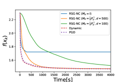
(a)

(b)

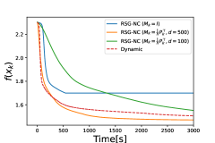
(c)

Figure 1: (a) Neural network with $l_{1}$-regularizer and sigmoid activation function, (b) Neural network with $l_{1}$-regularizer and ReLu activation function (c) Neural network with fused lasso and sigmoid activation function.

5.2.2 CNN with constraints

Since machine-learning problems often have highly nonconvex complicated objective functions consisting of numerous terms, we can not obtain the full gradient because of limitations on memory. In such a situation, we can use finite difference to calculate gradients. Here, we applied our method to this optimization problem that needs only the projected gradients $M_{k}^{\top}\nabla f\in\mathbb{R}^{d}$. If the reduced dimension $d$ is much smaller than original dimension $n$, it would save on time complexity. We optimized the CNN with the cross entropy loss under $l_{2}$ regularization, $\|x\|_{2}^{2}\leq 50$, on the MNIST dataset. We set the parameters $\varepsilon_{0},\delta_{1},\varepsilon_{2},\beta,\mu_{k}$ as follows:

$$\varepsilon_{0}=10^{-6},\delta_{1}=10^{-8},\varepsilon_{2}=10^{-4},\beta=0.8,\mu_{k}=\frac{1}{2\sqrt{s_{k}^{\top}(G_{k}^{\top}M_{k}M_{k}^{\top}G_{k})s_{k}}}.$$

For $M_{k}=\frac{1}{n}P_{k}^{\top}$, we set the step size as $h\in\{10^{2}n,10^{1}n,n\}$. For $M_{k}=I$, we set the step size as $h\in\{100,10,1\}$. Figure 2 shows that our method with random projection performs better than the deterministic version.

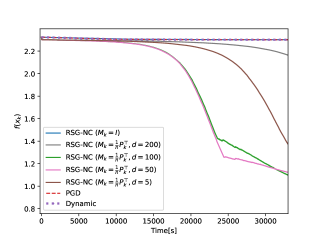
Figure 2: CNN with $l_{2}$-regularizer

6 Conclusion

We proposed new methods combining the random projection and gradient projection method. We proved that they globally converge under linear constraints and nonlinear constraints. When the original dimension is large enough, they converge in $O(\varepsilon^{-2})$. The numerical experiments showed some advantages of random projections as follows. First, our methods with randomness have the potential to obtain better solutions than those of their deterministic versions. Second, under non-smooth constraints, they did not become trapped at the boundary, whereas their deterministic versions did become trapped. Last, our methods performed well when the gradients could not be obtained directly. In the future, we would like to investigate the convergence rate of our algorithms in a non-smooth constraints setting.

7 Compliance with Ethical Standards

This work was partially supported by JSPS KAKENHI (23H03351) and JST ERATO (JPMJER1903). There is no conflict of interest in writing the paper.

References

- \bibcommenthead
- (1) Tibshirani, R., Saunders, M., Rosset, S., Zhu, J., Knight, K.: Sparsity and smoothness via the fused lasso. Journal of the Royal Statistical Society: Series B (Statistical Methodology) 67(1), 91–108 (2005)
- (2) Lee, D.D., Seung, H.S.: Learning the parts of objects by non-negative matrix factorization. Nature 401(6755), 788–791 (1999)
- (3) Zafar, M.B., Valera, I., Rogriguez, M.G., Gummadi, K.P.: Fairness constraints: Mechanisms for fair classification. In: Artificial Intelligence and Statistics, pp. 962–970 (2017)
- (4) Komiyama, J., Takeda, A., Honda, J., Shimao, H.: Nonconvex optimization for regression with fairness constraints. Proceedings of the Thirty-fifth International Conference on Machine Learning (ICML 2018) PMLR 80, 2737–2746 (2018)
- (5) Moldovan, T.M., Abbeel, P.: Safe exploration in markov decision processes. arXiv preprint arXiv:1205.4810 (2012)
- (6) Achiam, J., Held, D., Tamar, A., Abbeel, P.: Constrained policy optimization. In: International Conference on Machine Learning, pp. 22–31 (2017). PMLR
- (7) Kozak, D., Becker, S., Doostan, A., Tenorio, L.: A stochastic subspace approach to gradient-free optimization in high dimensions. Computational Optimization and Applications 79(2), 339–368 (2021)
- (8) Gower, R., Kovalev, D., Lieder, F., Richtárik, P.: Rsn: Randomized subspace newton. Advances in Neural Information Processing Systems 32 (2019)
- (9) Hanzely, F., Doikov, N., Nesterov, Y., Richtarik, P.: Stochastic subspace cubic newton method. In: International Conference on Machine Learning, pp. 4027–4038 (2020). PMLR
- (10) Fuji, T., Poirion, P., Takeda, A.: Randomized subspace regularized newton method for unconstrained non-convex optimization. arXiv preprint arXiv:2209.04170 (2022)
- (11) Chen, L., Hu, X., Wu, H.: Randomized fast subspace descent methods. arXiv preprint arXiv:2006.06589 (2020)
- (12) Berglund, E., Khirirat, S., Wang, X.: Zeroth-order randomized subspace newton methods. In: ICASSP 2022-2022 IEEE International Conference on Acoustics, Speech and Signal Processing (ICASSP), pp. 6002–6006 (2022). IEEE
- (13) Cartis, C., Fowkes, J., Shao, Z.: Randomised subspace methods for non-convex optimization, with applications to nonlinear least-squares. arXiv preprint arXiv:2211.09873 (2022)
- (14) Margossian, C.C.: A review of automatic differentiation and its efficient implementation. Wiley interdisciplinary reviews: data mining and knowledge discovery 9(4), 1305 (2019)
- (15) Cartis, C., Massart, E., Otemissov, A.: Bound-constrained global optimization of functions with low effective dimensionality using multiple random embeddings. Mathematical Programming, 1–62 (2022)
- (16) Rosen, J.B.: The gradient projection method for nonlinear programming. part i. linear constraints. Journal of the Society for industrial and applied mathematics 8(1), 181–217 (1960)
- (17) Du, D.-Z., Wu, F., Zhang, X.-S.: On rosen’s gradient projection methods. Annals of Operations Research 24(1), 9–28 (1990)
- (18) Rosen, J.B.: The gradient projection method for nonlinear programming. part ii. nonlinear constraints. Journal of the Society for Industrial and Applied Mathematics 9(4), 514–532 (1961)
- (19) Gao, Z., Lai, Y., Hu, Z.: A generalized gradient projection method for optimization problems with equality and inequality constraints about arbitrary initial point. Acta Mathematicae Applicatae Sinica 12, 40–49 (1996)
- (20) Wang, W., Hua, S., Tang, J.: A generalized gradient projection filter algorithm for inequality constrained optimization. Journal of Applied Mathematics 2013 (2013)
- (21) Johnson, W., Lindenstrauss, J.: Extensions of Lipschitz mappings into a Hilbert space. In: Hedlund, G. (ed.) Conference in Modern Analysis and Probability. Contemporary Mathematics, vol. 26, pp. 189–206. American Mathematical Society, Providence (1984)
- (22) Vershynin, R.: High-dimensional Probability: An Introduction with Applications in Data Science vol. 47. Cambridge university press, Cambridge (2018)
- (23) Gong, C., Liu, X., Liu, Q.: Automatic and harmless regularization with constrained and lexicographic optimization: A dynamic barrier approach. Advances in Neural Information Processing Systems 34, 29630–29642 (2021)