Improving Retrieval-Augmented Large Language Models via Data Importance Learning

Abstract

Retrieval augmentation enables large language models to take advantage of external knowledge, for example on tasks like question answering and data imputation. However, the performance of such retrieval-augmented models is limited by the data quality of their underlying retrieval corpus. In this paper, we propose an algorithm based on multilinear extension for evaluating the data importance of retrieved data points. There are exponentially many terms in the multilinear extension, and one key contribution of this paper is a polynomial time algorithm that computes exactly, given a retrieval-augmented model with an additive utility function and a validation set, the data importance of data points in the retrieval corpus using the multilinear extension of the model’s utility function. We further proposed an even more efficient $(\epsilon,\delta)$-approximation algorithm. Our experimental results illustrate that we can enhance the performance of large language models by only pruning or reweighting the retrieval corpus, without requiring further training. For some tasks, this even allows a small model (e.g., GPT-JT), augmented with a search engine API, to outperform GPT-3.5 (without retrieval augmentation). Moreover, we show that weights based on multilinear extension can be computed efficiently in practice (e.g., in less than ten minutes for a corpus with 100 million elements).

1 Introduction

Large language models (LLMs) consisting of neural networks with billions of parameters and trained on vast quantities of unlabelled text are the basis of unprecented progress in natural language processing tasks [6, 20, 21, 13]. With zero-shot or few-shot prompting, LLMs can be adopted for a wide range of diverse tasks, such as question answering [15] summarization [15, 2] and data imputation [17].

Drawbacks of large language models. LLMs, however, have two widely acknowledged disadvantages [1, 22]. Firstly, despite their impressive capabilities, LLMs actually perform badly on tail entities [1], which they have not seen at training time or cannot remember due to limitations of the network capacity. The second drawback is that with the ever-growing number of model parameters, training, and fine-tuning costs are exploding as well. As a rough estimate, it costs $80k - $1.6m to train a 1.5 billion parameter language model [25, 22, 29]. This makes it difficult to leverage LLMs for tasks that require regularly updated data or that regularly need to remove privacy-sensitive or copyright-protected data [3].

Retrieval-augmented models. To address such problems, retrieval-augmented (RAG) models have recently been proposed [12, 14, 8]. A typical retrieval-augmented model consists of two parts, a retriever $f_{ret}$ and a generator $f_{gen}$. Given a retrieval corpus $\mathcal{D}_{ret}=\{d_{1},\cdots,d_{M}\}$, the retriever $f_{ret}$ retrieves $K$ data points for an input $x_{i}$ as $f_{ret}(x_{i},\mathcal{D}_{ret})=\{d_{\alpha_{1}},d_{\alpha_{2}},...,d_{\alpha_{K}}\}$. Here, $\alpha_{k}$ denotes the rank of each data point in the retrieval corpus assigned by the retriever. The generator $f_{gen}$ then generates its prediction based on the input and the retrieved data points as evidence $f_{gen}(x_{i},f_{ret}(x_{i},\mathcal{D}_{ret}))$. Recent research indicates that incorporating external knowledge into LLMs improves their performance for various tasks and allows them to easily adapt to new knowledge [23, 30].

Figure 1: Data importance evaluation for retrieval-augmented models: The retriever $f_{ret}$ retrieves $K$ data points from the retrieval corpus $\mathcal{D}_{ret}$ and provides them to the answer generator $f_{gen}$. Our data importance evaluator learns weights for the data sources in the retrieval corpus based on the performance on a validation set $\mathcal{D}_{val}$. These weights are subsequently used to reweight or prune the data sources, and improve the model’s performance without further training.

Impact of data quality on retrieval-augmented LLMs. The performance of retrieval-augmented models is highly limited by the quality of the retrieved data points. For example, GPT-3 is able to give the correct answer “Frank Herbert” to the question “Who is the author of Old Rambling House?” with the help of a retrieved Wikipedia page  [28], which contains the sentence "Old Rambling House is a short story by American science fiction author Frank Herbert." However, it would with a high probability give the wrong answer if the retrieved page contained incorrect text such as “Old Rambling House is a short story by American science fiction author J. R. R. Tolkien.” Retrieval corpora are rarely clean in reality (especially if the underlying data comes from the web), and the origin of noise and errors in the data is difficult to track down [7, 5]. For example, according to recent estimates, $8.0\%$ to $38.5\%$ of labels in real-world datasets are corrupted [24]. In the domain of natural language processing, which relies on raw text, the rapidly growing number of use cases and an increasing amount of text have especially exacerbated data quality issues [5].

Learning the data importance of retrieval sources. Given this data quality problem, we propose to improve retrieval-augmented models by learning the data importance of retrieval sources. Let $U\left(\cdot\right)$ be the utility function of a retrieval-augmented model with a validation set $\mathcal{D}_{val}=\{x_{1},x_{2},...,x_{N}\}$, and let $\mathcal{D}_{ret}=\{d_{1},\cdots,d_{M}\}$ be the underlying retrieval corpus of $M$ data points. The performance of the model can be written as:

$$U(f_{gen},f_{ret},\mathcal{D}_{val},\mathcal{D}_{ret}):=\sum_{x_{i}\subseteq\mathcal{D}_{val}}U\left(f_{gen}(x_{i},f_{ret}(x_{i},\mathcal{D}_{ret}))\right)$$ (1)

Our goal to is find a subset $\mathcal{S}$ of the retrieval corpus $\mathcal{D}_{ret}$ that maximizes the utility function $U(f_{gen},f_{ret},\mathcal{D}_{val},\mathcal{S})$. We leave out $f_{gen}$, $f_{ret}$, and $\mathcal{D}_{val}$ from the notation and use $U(\mathcal{S})$ for readability. It is hard to solve this combinatorial optimization problem since it requires enumerating exponentially many possible subsets $\mathcal{S}$. One natural way is to change this problem to an optimization problem on continuous functions. Therefore, we define the multilinear extension of the utility function as:

$$\tilde{U}(w_{1},\cdots,w_{M}):=\sum_{\mathcal{S}\subseteq\mathcal{D}_{ret}}U\left(\mathcal{S}\right)\underbrace{\prod_{d_{i}\in\mathcal{S}}w_{i}\prod_{d_{i}\not\in\mathcal{S}}(1-w_{i})}_{P[\mathcal{S}]}$$ (2)

Here, $P[\mathcal{S}]$ denotes the probability of the sampled retrieval corpus $\mathcal{S}\subseteq\mathcal{D}_{ret}$ based on the weights $w_{1},\cdots,w_{M}$. Our goal is to find the optimal weights $w_{1},\cdots,w_{M}$ that maximize the multilinear extension of the utility function:

$$\max_{w_{1},\cdots,w_{M}\in[0,1]}\tilde{U}(w_{1},\cdots,w_{M})$$ (3)

The optimal weights can be found with textbook optimization methods like gradient descent. This, however, requires enumerating exponentially many sample sets, making the problem infeasible in practice. We tackle this challenge with the following main contributions of this paper:

• We present an efficient algorithm to compute weights for a large family (but not all) of retrieval-augmented models with additive utility functions. Our algorithm has polynomial time complexity and does not depend on the retrieval corpus size (Sections 2.1 & 2.2), even given that there are exponential many terms in Equation 2.

• We introduce an efficient estimation algorithm to compute the $(\epsilon,\delta)$-approximation of weights for a large family of retrieval-augmented models (Section 2.3).

• We experimentally demonstrate that retrieval augmentation and data evaluation based on multilinear extension improve the performance of large language models in question answering and data imputation tasks. The experiments demonstrate that with external retrieval knowledge, small language models can yield comparable performance to large language models. Furthermore, our evaluation shows that weights based on multilinear extension can identify noisy data and help models adapt to new sources of knowledge (Section 3.3).

• Our implementation of the algorithm illustrates that weights based on multilinear extension can be calculated very fast in practice, even for a large corpus with 100 million data points (Section 3.5).

• We provide the source code of our implementation and experiments under https://github.com/amsterdata/ragbooster.

2 Algorithms for Deriving Gradients

We can find the optimal weights for the multilinear extension of the utility function via computing the gradient of a particular weight $w_{i}$ based on a validation set $\mathcal{D}_{val}$:

$$\frac{\partial\tilde{U}}{\partial w_{i}} =\sum_{\mathcal{S}\subseteq\mathcal{D}_{ret}\backslash d_{i}}{\left(U(\mathcal{S}\cup\{d_{i}\})-U(\mathcal{S})\right)\cdot P[\mathcal{S}]}$$ (4)

$$=\sum_{x_{val}\in\mathcal{D}_{val}}\frac{1}{|\mathcal{D}_{val}|}\cdot\sum_{\mathcal{S}\subseteq\mathcal{D}_{ret}\backslash d_{i}}\underbrace{\left(U_{x_{val}}(\mathcal{S}\cup\{d_{i}\})-U_{x_{val}}(\mathcal{S})\right)\cdot P[\mathcal{S}]}_{G(x_{val},\ w_{i})}$$

$$=\frac{1}{|\mathcal{D}_{val}|}\cdot\sum_{x_{val}\in\mathcal{D}_{val}}G(x_{val},\ w_{i})$$

Infeasability of a naive implementation. However, computing the gradients in Equation 4 is challenging. A naive implementation would have to enumerate all possible subsets $\mathcal{S}$ for each validation tuple $x_{val}\in\mathcal{D}_{val}$ to compute the contribution of this subset $\mathcal{S}$ to the gradient value $G(x_{val},\ w_{i})$. Such a naive implementation is infeasible in practice due to its inherent exponential time complexity.

Efficient weight computation for retrieval-augmented models. As discussed before, we focus on a specific family of machine learning models, called retrieval-augmented (RAG) models. Retrieval-augmented models benefit from locality: the predictions of retrieval-augmented models for an input sample are only determined by the Top-$K$ closest data points in the retrieval corpus and the answer generator. Combined with additive utility functions (which are common for both classical KNN and state-of-the-art RAG models), this allows us to efficiently compute exact gradients within polynomial time complexity (Section 2.1 and Section 2.4). In Section 2.2, we show that we only have to consider a small subset of data points for each validation tuple and that the time complexity only depends on $K$ instead of the retrieval corpus size $M$ if we apply an $\epsilon$-approximation. Finally, we propose an $(\epsilon,\delta)$-approximation algorithm in Section 2.3 to calculate gradients for general utility functions.

2.1 Exact Gradient Calculation for Models with an Additive Utility Function

A textbook $K$-nearest neighbor classifier and many state-of-the-art retrieval-augmented models [14] can be viewed as models with additive utility functions. In this section, we present a polynomial time complexity algorithm to compute the exact gradient of the weights of the multilinear extension of the utility function. We follow existing work [10] to define the additive utility function of a retrieval-augmented model as:

$$U_{x_{val}}(\mathcal{S})=\frac{1}{K}\sum_{k=1}^{\min{(K,|\mathcal{S}|)}}{U_{x_{val}}(f_{gen}(d_{\alpha_{k}^{x_{val}}(\mathcal{S})}))}$$ (5)

Here, $\alpha_{k}^{x_{val}}(\mathcal{S})$ represents the index of the data point, which is the $k$th closest to $x_{val}$ among all the data points retrieved by $f_{ret}$ from $\mathcal{S}$. From now on, we abbreviate $\alpha_{k}^{x_{val}}(\mathcal{S})$ to $\alpha_{k}$. $U_{x_{val}}(f_{gen}(d_{\alpha_{k}^{x_{val}}(\mathcal{S})}))$ denotes the utility function for the output generated based on the validation tuple $x_{val}$ and the single data point $d_{\alpha_{k}^{x_{val}}}$. We assume that the possible values of $U\left(\cdot\right)$ function are within a countable finite set $\mathcal{V}$, where $|\mathcal{V}|=V$, and leave out $f_{gen}$ from the notation for readability in the following. In this scenario, we can provide an algorithm with PTIME time complexity in Appendix A. The overall time complexity of the algorithm is $\mathcal{O}{\left(N\cdot(M\log{M}+MK^{2}+MKV)\right)}$

2.2 $\epsilon$-approximation Algorithm for Calculating Exact Gradient Values

The overall time complexity for computing gradients for models with an additive utility function is $\mathcal{O}{\left(N\cdot(M\log{M}+MK^{2}+MKV)\right)}$. In this section, we show that if we are allowed to do $\epsilon$-approximations, we can significantly speed up the calculation of the gradients $\frac{\partial\tilde{U}}{\partial w_{i}}$. We will only introduce the main idea here, leaving the details in Appendix B.

Theorem 2.1.

If we calculate the $\epsilon$-approximation $\hat{G}(x_{val},\ w_{i})$ for the each $G(x_{val},\ w_{i})$, we can get the $\epsilon$-approximation for $\frac{\partial\tilde{U}}{\partial w_{i}}$ as the average of $\hat{G}(x_{val},\ w_{i})$.

Proof.

See Section E.1.∎

Our next step is to detail how to compute the $\epsilon$-approximation for $G(x_{val},\ w_{i})$. One observation is that the absolute value $G(x_{val},\ w_{i})$ is bounded by the sum of the probabilities of the data points $d_{i}$ in the $K$-nearest neighbor set of $x_{val}$. Notice that for a data point with a lower rank, the probability of it being in the $K$-nearest neighbor set is smaller. Therefore we can define the boundary point $d_{b}$ of the retrieval corpus.

Definition 2.1.

(Boundary Point) Given a validation tuple $x_{val}$ and the retrieval corpus $\mathcal{D}_{ret}=\{d_{1},\cdots,d_{M}\}$ ranked with respect to $x_{val}$, the boundary point $d_{b}$ is the data point with the highest rank in the sorted corpus such that any data point that has a lower rank than $d_{b}$ has a probability less than $\epsilon$ to be in the $K$-nearest neighbor set of $x_{val}$.

In practice, after we rank the corpus with respect to a validation tuple, we can use binary search to find the boundary point. After we find this boundary point $d_{b}$, we can use 0 as the $\epsilon$-approximation for the gradient for data points with a lower rank as $\hat{G}(x_{val},\ w_{i})=0$ for $i\in\{b,...,M\}$. It is because the probability of those data points being in the $K$-nearest neighbor set is less than $\epsilon$. In the following, we will show the approximation for data points with a higher rank.

Theorem 2.2.

Given the validation tuple $x_{val}$, the retrieval corpus $\mathcal{D}_{ret}=\{d_{1},...,d_{M}\}$, the boundary point $d_{b}$, and the weights $W=\{w_{1},...,w_{M}\}$, if we have an algorithm $\mathcal{A}$ to calculate the $G(x_{val},w_{i})=\mathcal{A}(x_{val},\mathcal{D}_{ret},W)$, then $\hat{G}(x_{val},\ w_{i})=\mathcal{A}(x_{val},\{d_{1},...,d_{b}\},\{w_{1},...,w_{b}\})$ is the $\epsilon$-approximation for $G(x_{val},w_{i})$.

Proof.

See Section E.2∎

From Theorem 2.2, we can compute the $\epsilon$-approximation for every data point by discarding the outlier points $\{d_{b},d_{b+1},...,d_{M}\}$. This reduces the time complexity from $\mathcal{O}{\left(N\cdot(M\log{M}+MK^{2}+MKV)\right)}$ to $\mathcal{O}{\left(N\cdot(B\log{B}+BK^{2}+BKV)\right)}$ where $B$ is the rank of the boundary point.

Theorem 2.3.

If the value of all $w_{i}$ is greater than a certain constant $\lambda$, then the index of the boundary point $B$ is $\mathcal{O}(K)$.

Proof.

See Section E.3∎

The above theorem shows that if all weights $W$ are greater than a certain constant, the scale of $B$ is only related to $K$ instead of the size of the retrieval corpus $M$. It means that even though we may have millions of data points in the retrieval corpus, we only have to consider $O(K)$ data points with the highest rank for a validation tuple. The overall time complexity for computing the approximate gradients for models with additive utility functions is $\mathcal{O}{\left(N\cdot(K\log{K}+KKV)\right)}=\mathcal{O}{\left(N\cdot K^{2}\cdot V\right)}$. This significantly speeds up their computation.

2.3 $(\epsilon,\delta)$-approximation Algorithm for Models with General Utility Functions

Next, we provide a solution for efficiently approximating gradients for retrieval-augmented models with a general utility function. According to what we proposed in the previous section, for every validation tuple, we can find the boundary point of the retrieval corpus. When a point has a smaller rank score than the boundary point, the epsilon approximation is 0. Using the Markov chain Monte Carlo method, we can calculate an approximation of the gradients for a retrieval-augmented model with a general utility function. In light of the fact that 0 is the approximate value for most points, we only need to perform MCMC on a small number of data points. Detailed proofs and algorithms are provided in appendix D.

2.4 Projected Gradient Descent for Weights on a Data Source Level

Exact gradients for a grouped retrieval corpus. In the previous section, we introduced the algorithm for calculating gradients for weights for the multilinear extension of the utility function. We also proved that each validation tuple only contributes gradients to a small part of the retrieval corpus. A further problem is how to evaluate the quality of the data points which are not retrieved for the validation tuples. In real-world ML applications, a retrieval corpus is commonly generated from various data sources. For example, data points in the retrieval corpus may come from the same labeler, the same websites, or the same database. As a consequence, we can evaluate data quality at this level, which we call the source level. This has the additional advantage that we do not have to inspect every data point before identifying if the data is useful. We formulate the corresponding problem as follows. Given a series of data sources for the retrieval corpus $\mathcal{O}_{ret}=\{o_{1},o_{2},...,o_{M}\}$, the generated retrieval corpus can be represented as a function of these sources ${D}_{ret}=\bigcup_{i=1}^{M}{f_{source}(o_{i})}$. We detail how to compute the exact gradient of the weights for the K-Nearest Neighbor classifier and a grouped corpus in Appendix C. The time complexity of the algorithm is $\mathcal{O}\left(N\cdot T^{2}\cdot M^{2}\right)$, where $T$ is the size of the generated retrieval corpus.

Projected gradient descent for weights on a grouped corpus. In general, given the retrieval corpus and the validation set, we can use a textbook batch gradient descent algorithm to find the optimal weights for the data points in the retrieval corpus. From the previous paragraph, we can see that computing the exact gradient values for a grouped retrieval corpus with several data sources can be computationally expensive. Therefore, we propose a projected gradient descent algorithm to efficiently learn the optimal weights for retrieval corpus generated from data sources. Given the generated retrieval corpus represented as a function of the sources $\{o_{1},o_{2},...,o_{M}\}$, ${D}_{ret}=\bigcup_{i=1}^{M}{f_{source}(o_{i})}$, we assign a weight to each data point in the generated retrieval corpus ${D}_{ret}$. Suppose there are $m_{i}$ data points in $f_{source}(o_{i})$, we assign the weights $\{w_{i,1}.w_{i,2},...,w_{i,m_{i}}\}$ to each data point in $f_{source}(o_{i})$. The original optimization problem can be relaxed to a constrained optimization problem as detailed below:

$$\max_{w_{1,1},\cdots,w_{M,m_{M}}\in[0,1]}\tilde{U}(\ w_{1,1},...,w_{M,m_{M}})$$ (6)

$$\begin{array}[]{r@{\quad}r@{}l@{\quad}l}s.t.&w_{1,1}=w_{1,2}=\cdots&=w_{1,m_{1}}\\ &w_{2,1}=w_{2,2}=\cdots&=w_{2,m_{2}}\\ &\cdots\\ &w_{M,1}=w_{M,2}=\cdots&=w_{M,m_{M}}\\ \end{array}$$

To find the optimum of this function, we use the existing algorithm for a non-grouped corpus to compute the gradient of the weight for each $w_{i,j}$. After we update the parameters using the gradients, we project the updated $w_{i,j}$ to satisfy the constraints by computing $\hat{w_{i}}=\frac{1}{\alpha}\sum{w_{i,j}}$ and set every $w_{i,j}$ to $\hat{w_{i}}$. Therefore, we can utilize the algorithm introduced in Section 2.2 to calculate the gradient and then compute the average. For retrieval-augmented models with additive utility functions, the time complexity becomes $\mathcal{O}{\left(N\cdot K^{2}\cdot V+T\right)}$.

3 Experimental Evaluation

We conduct a series of experiments for question answering and data imputation tasks. We confirm in Section 3.1 that retrieval augmentation enhances the performance of large language models. Section 3.2 and Section 3.3 show that the multilinear extension weights help us identify noisy/incorrect data in the retrieval corpus, and that pruning or reweighting the retrieval corpus accordingly improves performance without the need to fine-tune the underlying model. The runtime of the algorithm is examined in Section 3.5, where we showcase that the weights can be computed very fast in practice. We provide the source code of our implementation and experiments under https://github.com/schelterlabs/retrieval_importance.

Datasets and tasks. For question answering, we leverage the WikiFact [15] dataset, in which questions are extracted from Wikipedia pages using relation pairs. The answer to each question in this dataset can be found on Wikipedia. For example, for the relation "author", a question is "The author of Nimmer on Copyright is ?". We filter out relations with less than 500 questions and use each of the remaining 70 relations as a separate downstream task. In data imputation, the task is to predict missing values of a relational table [17]. We experiment with two common benchmark datasets for this task: restaurant, where the city column of a table about restaurants must be imputed, and buy, where we have to impute the manufacturer column in a table about electronics products. For each experimental run on a question answering or data imputation task, we randomly split the dataset into validation dataset and test dataset with an equal number of tuples. We repeat this for 64 different random seeds, and report the mean accuracy. For the zero-shot baselines in the imputation tasks, we use the prompts suggested in [17].

Language models. We leverage the language model GPT-JT [27, 26] with 6 billion parameters, which we enhance with retrieval augmentation. As a reference, we compare this to the language model “text-davinci-003” (to which we refer to as GPT-3.5) from OpenAI’s commercial GPT-3.5 family [19]. For both language models, we generate predictions with zero-shot or few-shot prompting, without further fine-tuning.

Retrieval augmentation. We leverage the Microsoft Bing search engine [16] to generate a retrieval corpus for each task. We create a query from each validation/test sample (e.g., the question to answer) and retrieve the first 50 websites together with their textual snippets provided by Bing as retrieved data points for the sample. We sort these data points according to the ranking score provided by Bing. We create a few-shot prompt from each retrieved data point, and generate an answer for the corresponding validation sample via GPT-JT. We decide on the final prediction via a majority vote using the generated answers from the top-$K$ websites.

Reweighting or pruning the retrieval corpus. In experiments which reweight or prune the retrieval corpus based on multilinear extension weights, we proceed as follows. We choose K = 10 and set the initial weight to 0.5. We group the retrieved websites by their domain name, and run the projected gradient descent algorithm from Section 2.4 for 50 iterations with a learning rate of 500 on the validation dataset to compute the optimal weights. Next, for reweighting, we compute the expectation of the accuracy on the test set by randomly sampling the retrieved data points 32 times based on the learned weights to form the retrieval corpus. For pruning, we remove retrieved data points with a learned weight below a certain threshold (tuned on the validation set) before computing predictions on the test set via majority vote. We use the leave-one-out (LOO) error as a baseline to refine the retrieval corpus. We compute the change in accuracy for the removal of each individual data source and finally remove all data sources with a LOO error below a certain threshold (tuned on the validation set) before computing predictions on the test set.

3.1 Benefits of Retrieval Augmentation

Experimental setup. The aim of this experiment is to confirm the well-known fact that retrieval augmentation alone already enhances the performance of language models. We compare the performance of GPT-3.5 without retrieval augmentation to the performance of GPT-JT with retrieval augmentation on the question answering and data imputation tasks.

Results and discussion. The results for question answering are shown in Table 1a. The mean accuracy of GPT-3.5 over all 70 relations is 0.33, which outperforms the mean accuracy of 0.21 achieved by GPT-JT standalone. However, retrieval augmentation raises the mean accuracy of GPT-JT to 0.33, making it competitive with the 30x larger GPT-3.5. The smaller model even outperforms the larger model in the majority of relations (39 out of 70, detailed results available in Appendix F). We encounter the analogous behavior for data imputation in Table 2, where retrieval augmentation (vanilla) makes the small GPT-JT model competitive with the 30x larger GPT-3.5 model, and even outperforms it on both datasets.

Table 1: Average accuracy for question answering on Wikifact. A small language model with retrieval augmentation and learned multilinear extension weights outperforms a large model with 30 times more parameters.

GPT-JT (6B)	GPT-JT (6B) w/ Retrieval			GPT-3.5 (175B)
	K = 1	K = 10	K = 50
0.214	0.332	0.333	0.293	0.339

(a) Benefits of retrieval augmentation.

GPT-JT (6B) w/ Retrieval				GPT-3.5 (175B)
vanilla	+ loo	+ reweight	+ prune
0.333	0.358	0.380	0.392	0.339

(b) Benefits of weight-based reweighting and pruning.

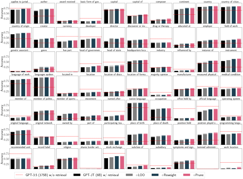
Figure 2: Accuracy for question answering on the 70 relations from WikiFact.

3.2 Improving Performance with Multilinear Extension Weights

Experimental setup. Next, we showcase that pruning or reweighting the retrieval corpus based on multilinear extension weights importance improves performance without having to fine-tune the underlying model. We group the retrieved websites by domain and refine the corpus as detailed earlier.

Results and discussion. The results for question answering are shown in Table 1b (detailed results inFigure 2 and Appendix G), and confirm that reweighting and pruning using the learned weights increases test accuracy. The mean accuracy of the GPT-JT model retrieval augmentation increases from 33.3% to 37.7% after pruning (and to 36.9% after reweighting) using the multilinear extension weights, and it clearly outperforms the state-of-the-art GPT-3.5 model with 175 billion parameters. In all 70 relations, the performance improved using multilinear extension weights by removing 71.5% of the retrieval corpus on average. Analogously, we find that the performance in the data imputation tasks is improved by pruning based on the learned weights importance as well (Table 2). For both datasets, the smaller model outperforms GPT-3.5 by more than 5% in test accuracy. These results confirm that the performance of retrieval-augmented models can be further optimized by evaluating the quality and reliability of real-world data sources in their underlying corpus.

Table 2: Average accuracy for data imputation on buy and restaurant.

Dataset	GPT-JT (6B)	GPT-JT (6B) w/ retrival				GPT-3.5 (175B)
		vanilla	+loo	+reweight	+prune
Buy	0.102	0.789	0.808	0.815	0.813	0.764
Restaurant	0.030	0.746	0.756	0.760	0.761	0.463

3.3 Mitigating the Impact of Noise in the Retrieval Corpus

Table 3: Accuracy improvements for GPT-JT (6B) with retrieval augmentation on a noisy corpus.

CLEAN CORPUS	DIRTY CORPUS
	vanilla	+ loo	+ reweight	+ prune
0.333	0.270	0.311	0.330	0.335

Experimental setup. The aim of the following experiment is to demonstrate how the learned weights assist us with mitigating the impact of noise in the retrieval corpus. To achieve this, we manually inject noise into the retrieval corpus of the question-answering task as follows. We create five copies of the retrieval corpus for each question with noise levels ranging from $0\%$ to $80\%$ (resulting in around 250 retrieved websites per question, of which $40\%$ are corrupted). To inject noise, we randomly replace the correct answer in the retrieved websites with an incorrect one according to the noise level. Then, for each copy, we randomly split the corpus into ten sources according to rank. Now we have $5\cdot 10$ different sources in total with different noise levels. We expect a performance drop when using the dirty corpus and aim to demonstrate how data evaluation can help us restore performance.

Results and discussion. As shown in Table 3, the performance drops from 33.3% on the clean corpus to 27.0% on the dirty corpus with injected noise. Using the leave-one-out error to remove noise sources improves performance to 31.1%. Both reweighting and pruning using learned weights drastically improve the performance on the dirty corpus and both enhance the performance by over 33.0% on the dirty corpus. Pruning even results in a better performance of 33.5% compared to the clean corpus without pruning. The results show that even if we are faced with a situation where nearly half of the retrieval corpus is noisy, multilinear extension weights can help the model reach performance comparable to the clean corpus.

GPT-JT (6B) w/  Retrieval	GPT-JT (6B) w/  Retrieval + Fabricated Data				GPT-3.5 (175B)
	vanilla	+loo	+reweight	+prune
0.333	0.382	0.399	0.410	0.418	0.339

tableAccuracy impact of additional fabricated data sources for question answering on Wikifact.

figureRuntime per epoch on corpora with up to 100M elements.

3.4 Handling Auto-Generated Data Sources in the Retrieval Corpus

Experimental setup. Next, we illustrate how learned weights allows us to handle new sources in the retrieval corpus for question answering. We manually generate five synthetic Wikipedia pages for each question using the OpenAI “text-davinci” generator. We adopt the real Wikipedia pages as a few-shot example, add the fabricated sources to the retrieval corpus and give them the highest rank among the websites. We aim to show that when new knowledge is added to the corpus, the learned weights help us to utilize the sources based on their quality.

Results and discussion. Section 3.3 shows the results of this experiment. We find that adding fabricated Wikipedia pages to the corpus increases the accuracy from 33.3% to 38.2%. This is due to the fact that the OpenAI model itself can reach 33.9% and most Wikipedia pages contain the correct information if the model memorizes the answer. We see, however (e.g., for the relation "place of death"), that adding generated Wikipedia pages will decrease the performance from 38.3% to 33.8%. Using LOO to prune the retrieval corpus improves performance by 39.9% on average. Reweighting or pruning using the learned multilinear extension weights achieves the highest accuracy of 41.0% and 41.8%, improving the performance on the corpus without fabricated Wikipedia sources. The results show that the learned weights help the model to easily adapt to new knowledge sources without further training.

3.5 Computational Performance

Experimental setup. Finally, we illustrate that the weights can be computed very fast in practice. For that, we implement our approach in Rust (with a Python frontend), and apply several performance optimizations to the code such as parallelization, memory pre-allocation and re-use, operator fusion, and predication [4, 18]. We run the experiments on consumer hardware (a machine with a four-core Intel i7-8569U CPU @2.80GHz, 16GB of RAM, and MacOS 12.6). We measure the runtime of our implementation on three relations from the Wikifact dataset (“author”, “place-of-birth”, “currency”), which contain 1,700-2,700 questions each, with 50 corresponding retrieved answers per question. We additionally run experiments on a synthetic retrieval corpus whose size $M=N\cdot b$ we scale up from 50,000 to 100,000,000 (with a validation set size $N$ from 1,000 to 1000,000 times $b=[50,100]$ retrieved data points per sample). We run each configuration with one, two, and four threads, repeat each run seven times, and measure the mean execution time per epoch.

Results and discussion. For the relations from WikiFact, a gradient update only takes between two and four milliseconds. We plot the results for the synthetic corpus in Section 3.3. The x-axis is the size of the retrieval corpus $M=N\cdot b$ (size $N$ of the validation set times the number of retrieved data points per sample $b$) and the y-axis denotes the mean runtime in milliseconds with a logarithmic scale. We see that with all four cores, we can finish an epoch for corpora with up to 10 million elements with a sub-second runtime. Even for the largest corpus with 100 million elements, an epoch can be conducted in 6.3 seconds on consumer hardware. Furthermore, we find that the runtime grows linearly with the size of the retrieval corpus and that our implementation easily benefits from parallelism when multiple cores are utilized. This showcases that data refinement using multilinear extension weights is computationally cheaper than model fine-tuning, which (in many cases) has to conduct an expensive backpropagation of errors through the underlying model.

4 Conclusion

We presented efficient algorithms to compute the optimal weights that maximize the multilinear extension of the utility function and use them to refine the retrieval corpus for retrieval-augmented large language models. Overall, our results illustrate that the learned weights are a powerful metric for evaluating the quality of the retrieval corpus and that retrieval-augmented models can be enhanced by only pruning the retrieval corpus without further training the underlying model. Furthermore, the weights can be computed efficiently even for a large retrieval corpus, and allow us to easily adapt predictions in cases where new sources are added to the retrieval corpus.

Appendix A Exact Gradient Calculation for Models with an Additive Utility Function

We will first introduce two building blocks to help calculate the gradient:

Definition A.1.

(Subset Probability) Given the retrieval corpus $\mathcal{D}_{ret}=\{d_{1},...,d_{M}\}$ and the weights $W=\{w_{1},...,w_{M}\}$, subset probability $P_{k}(a,b)$ is the sum of the probability of subsets with a size of $k$ from $\mathcal{D}^{\prime}=\{d_{a},d_{a+1},...,d_{b}\}$.

$$P_{k}(a,b)=\sum_{|\mathcal{S}|=k,\mathcal{S}\subseteq\mathcal{D}^{\prime}}\prod_{d_{i}\in\mathcal{S}}w_{i}\prod_{d_{i}\not\in\mathcal{S}}(1-w_{i})$$ (7)

We only use the subset probability values $P_{\cdot}{(1,\cdot)}$ and $P_{\cdot}{(\cdot,M)}$. We compute these subset probability values within $\mathcal{O}(MK)$ time complexity, leveraging previous work on efficiently computing Poisson-binomial distribution values [9].

Definition A.2.

(Boundary Value Probability) Given the validation tuple $x_{val}$, the retrieval corpus $\mathcal{D}_{ret}=\{d_{1},...,d_{M}\}$, the weights $W=\{w_{1},...,w_{M}\}$ and the possible value set $\mathcal{V}$ of the utility function, the boundary value probability $B_{k}(i,e)$ is the sum of the probability of all subsets $\mathcal{S}$ sampled from $\mathcal{D}^{\prime}=\{d_{i},d_{i+1},...,d_{M}\}$ whose $k$-th element $d_{\alpha_{k}{(\mathcal{S})}}$ is evaluated as $e$.

$$B_{k}(i,e)=\sum_{U_{x_{val}}(d_{\alpha_{k}{(\mathcal{S})}})=e,\mathcal{S}\subseteq\mathcal{D}^{\prime}}\prod_{d_{i}\in\mathcal{S}}w_{i}\prod_{d_{i}\not\in\mathcal{S}}(1-w_{i})$$ (8)

This term can be calculated via dynamic programming:

$$B_{k}(i,e)=\left\{\begin{array}[]{lr}B_{k}(i+1,e)*(1-w_{i})+\mathbb{I}\{U_{x_{val}}(d_{i})=e\}*w_{i}&k=1\\ B_{k}(i+1,e)*(1-w_{i})+B_{k-1}(i+1,e)*w_{i}&k>1\end{array}\right.$$ (9)

To make Equation (9) correct for every $k\in[1,K]$, $i\in[1,M]$ and $e\in\mathcal{V}$, we initialize the boundary value to $B_{k}(M+1,e)=0$ for $k\in[1,K],e\in\mathcal{V}$. The time complexity of computing the boundary value probability using the above equation is $\mathcal{O}{(MKV)}$.

With these two building blocks, we are able to calculate the exact value of $G(x_{val},\ w_{i})$. We examine two situations.

(1) $|\mathcal{S}|<K$

In this case, the size of sampled retrieval corpus $\mathcal{S}$ is smaller than $K$. Therefore, including the data point $d_{i}$ in $\mathcal{S}$ does not expel any data point from the $K$-nearest neighbor set. Thus,

$$U_{x_{val}}(\mathcal{S}\cup\{d_{i}\})-U_{x_{val}}(\mathcal{S})=\frac{U_{x_{val}}(d_{i})}{K}$$ (10)

The sum of the probability of the respective subsets $\mathcal{S}$ equals the probability of selecting subsets with sizes less than $K$ from $\{d_{1},...,d_{i-1},d_{i+1},...,d_{M}\}$. The gradient for these sampled subsets $\mathcal{S}$ can be written as:

$$G_{1}(x_{val},\ w_{i}) =\sum_{|S|<K,\mathcal{S}\subseteq\mathcal{D}_{ret}\backslash d_{i}}\frac{U_{x_{val}}(d_{i})}{K}\cdot P[\mathcal{S}]$$ (11)

$$=\frac{U_{x_{val}}(d_{i})}{K}\cdot\sum_{k^{\prime}=0}^{K-1}\sum_{j=0}^{k^{\prime}}P_{j}{(1,i-1)}\cdot P_{k^{\prime}-j}{(i+1,M)}$$

The time complexity of computing all $G_{1}(x_{val},\ w_{i})$ using the above equation is $\mathcal{O}{(MK^{2})}$.

(2) $|\mathcal{S}|\geq K$

In this scenario, adding data point $d_{i}$ to the sampled corpus $\mathcal{S}$ expels data point $d_{\alpha_{K}(S)}$ from the $K$-nearest neighbor set. The corresponding difference in the utility function is:

$$U_{x_{val}}(\mathcal{S}\cup\{d_{i}\})-U_{x_{val}}(\mathcal{S})=\frac{U_{x_{val}}(d_{i})-U_{x_{val}}(d_{\alpha_{K}(S)})}{K}$$ (12)

The gradient contributed by the corresponding sampled subsets can be calculated by enumerating the data points that would be expelled from the $K$-nearest neighbor set. Suppose $d_{k^{\prime}}$ is the one to be expelled, then the sum of the probability of the corresponding subsets $\mathcal{S}$ equals selecting $K$ data points from $\{d_{1},...,d_{i-1},d_{i+1},...,d_{k^{\prime}}\}$. Therefore, the sum of the gradient can be written as:

$$G_{2}(x_{val},\ w_{i})= \sum_{|S|\geq K,\mathcal{S}\subseteq\mathcal{D}_{ret}\backslash d_{i}}\frac{U_{x_{val}}(d_{i})-U_{x_{val}}(d_{\alpha_{K}(S)})}{K}\cdot P[\mathcal{S}]$$ (13)

$$= \sum_{e\in\mathcal{V}}\frac{U_{x_{val}}(d_{i})-e}{K}\cdot\sum_{j=0}^{K-1}P_{j}{(1,i-1)}\cdot B_{K-j}{(i+1,e)}$$

The time complexity of computing all $G_{2}(x_{val},\ w_{i})$ using the above equation is $\mathcal{O}{(MKV)}$. The exact gradient values $G(x_{val},\ w_{i})$ can be computed by the sum of $G_{1}(x_{val},\ w_{i})$ and $G_{2}(x_{val},\ w_{i})$. The detailed algorithm is shown in Algorithm 1. The overall time complexity of the algorithm is $\mathcal{O}{\left(N\cdot(M\log{M}+MK^{2}+MKV)\right)}$

Algorithm 1 Exact Gradient Calculation for Models with an Additive Utility Function

  Input: $\mathcal{D}_{ret}=\{d_{1},...,d_{M}\}$, retrieval corpus; $\mathcal{D}_{val}=\{x_{1},\cdots,x_{N}\}$, validation set; $W=\{w_{1},...,w_{M}\}$, weights of data points;

  Output: $\{g_{1},\cdots,g_{M}\}$, gradients of weights;

  $\{g_{1},...,g_{M}\}\leftarrow 0$

  for  $x_{val}\in\mathcal{D}_{val}$ do

     $\{d_{\pi_{1}},\cdots,d_{\pi_{M}}\}\leftarrow$ SortByRankingScore($\mathcal{D}_{ret},x_{val}$)

     $P\leftarrow$ ComputeSubsetProb$(W,\pi)$

     $B,\mathcal{V}\leftarrow$ ComputeBVProb$(W,\pi,\mathcal{D}_{ret},x_{val})$

     for $i\leftarrow 1\ to\ M$ do

        $\mu_{1}\leftarrow\frac{U_{x_{val}}(d_{\pi_{i}})}{K}\cdot\frac{1}{N}$

        for $k^{\prime}\leftarrow 0\ to\ K-1$ do

           for $j\leftarrow 0\ to\ k^{\prime}$ do

              $g_{\pi_{i}}\leftarrow g_{\pi_{i}}+\mu_{1}\cdot P_{j}{(1,i-1)}\cdot P_{k^{\prime}-j}{(i+1,M)}$

           end for

        end for

        for $e\in\mathcal{V}$ do

           $\mu_{2}\leftarrow\frac{U_{x_{val}}(d_{\pi_{i}})-e}{K}\cdot\frac{1}{N}$

           for $j\leftarrow 0\ to\ K-1$ do

              $g_{\pi_{i}}\leftarrow g_{\pi_{i}}+\mu_{2}\cdot P_{j}{(1,i-1)}\cdot B_{K-j}{(i+1,e)}$

           end for

        end for

     end for

  end for

Appendix B $\epsilon$-approximation Algorithm for Calculating Exact Gradient Value

The overall time complexity for computing gradients for models with an additive utility function is $\mathcal{O}{\left(N\cdot(M\log{M}+MK^{2}+MKV)\right)}$. In this section, we show that if we are allowed to do $\epsilon$-approximations, we can significantly speed up the calculation of the gradients.

Theorem B.1.

If we calculate the $\epsilon$-approximation $\hat{G}(x_{val},\ w_{i})$ for the each $G(x_{val},\ w_{i})$, we can get the $\epsilon$-approximation for $\frac{\partial\tilde{U}}{\partial w_{i}}$ as the average of $\hat{G}(x_{val},\ w_{i})$.

Proof.

See Section E.1.∎

Our next step is to detail how to compute the $\epsilon$-approximation for $G(x_{val},\ w_{i})$. The variable $\phi_{\mathcal{S},x_{val}}\left(\ d_{i}\right)=(U_{x_{val}}(\mathcal{S}\cup\{d_{i}\})-U_{x_{val}}(\mathcal{S}))$ equals zero if $d_{i}$ is not in the $K$-nearest neighbor set of $\mathcal{S}\cup\{d_{i}\}$. This is due to the fact that adding the data point $d_{i}$ to the corpus will not change the data points retrieved by the model. Assuming that the utility function value is within the range of $[0,1]$, Equation 4 can be written as:

$$\left|G(x_{val},\ w_{i})\right| =\left|\sum_{\mathcal{S}\subseteq\mathcal{D}_{ret}\backslash d_{i}}\mathbb{I}\left\{d_{i}\in\operatorname{top_{K}}(\mathcal{S}\cup\{d_{i}\})\right\}\cdot\underbrace{\phi_{\mathcal{S},x_{val}}\left(\ d_{i}\right)}_{\in[-1,1]}\cdot P(\mathcal{S})\right|$$ (14)

$$\leq\sum_{\mathcal{S}\subseteq\mathcal{D}_{ret}\backslash d_{i}}\mathbb{I}\left\{d_{i}\in\operatorname{top_{K}}(\mathcal{S}\cup\{d_{i}\})\right\}\cdot P[\mathcal{S}]$$

From Equation 14 we can see that the absolute value $G(x_{val},\ w_{i})$ is bounded by the sum of the probabilities of the data points $d_{i}$ in the $K$-nearest neighbor set of $x_{val}$. The probability of data point $d_{i}$ to be in the $K$-nearest neighbor set equals the probability of less than $(K-1)$ points with higher ranks appearing in $\mathcal{S}$. The latter can be modeled by a Poisson-binomial distribution. Suppose that the retrieval corpus $\{d_{1},d_{2},\cdots,d_{M}\}$ is ranked with respect to $x_{val}$, then the gradient can be bounded via the Chernoff bound for $\mu_{i}>K-1$, where $\mu_{i}=\sum_{k=0}^{i-1}w_{k}$:

$$\left|G(x_{val},\ w_{i})\right| \leq P[{\bf PB}(w_{1},w_{2},\cdots,w_{i-1})\leq K-1] \leq\exp(-\frac{(\mu_{i}-K+1)^{2}}{2\mu_{i}})$$ (15)

Notice that for a data point with a lower rank, the probability of it being in the $K$-nearest neighbor set is smaller. Therefore we can define the boundary point $d_{b}$ of the retrieval corpus.

Definition B.1.

(Boundary Point) Given a validation tuple $x_{val}$ and the retrieval corpus $\mathcal{D}_{ret}=\{d_{1},\cdots,d_{M}\}$ ranked with respect to $x_{val}$, the boundary point $d_{b}$ is the data point with the highest rank in the sorted corpus such that any data point that has a lower rank than $d_{b}$ has a probability less than $\epsilon$ to be in the $K$-nearest neighbor set of $x_{val}$.

In practice, after we rank the corpus with respect to a validation tuple, we can use binary search to find the boundary point.

$$\min_{b}{\left[\left(\exp(-\frac{(\mu_{b}-K+1)^{2}}{2\mu_{b}})<\epsilon\right)\land\left(\mu_{b}>K-1\right)\right]}$$ (16)

After we find this boundary point $d_{b}$, we can use 0 as the $\epsilon$-approximation for the gradient for data points with a lower rank. $\hat{G}(x_{val},\ w_{i})=0$ for $i\in\{b,...,M\}$, because the probability of those data points being the $K$-nearest neighbor is less than $\epsilon$. In the following, we detail the approximation for data points with a higher rank.

Theorem B.2.

Given the validation tuple $x_{val}$, the retrieval corpus $\mathcal{D}_{ret}=\{d_{1},...,d_{M}\}$, the boundary point $d_{b}$, and the weights $W=\{w_{1},...,w_{M}\}$, if we have an algorithm $\mathcal{A}$ to calculate the $G(x_{val},w_{i})=\mathcal{A}(x_{val},\mathcal{D}_{ret},W)$, then $\hat{G}(x_{val},\ w_{i})=\mathcal{A}(x_{val},\{d_{1},...,d_{b}\},\{w_{1},...,w_{b}\})$ is the $\epsilon$-approximation for $G(x_{val},w_{i})$.

Proof.

See Section E.2∎

From Theorem B.2, we can compute the $\epsilon$-approximation for every data point by discarding the outlier points $\{d_{b},d_{b+1},...,d_{M}\}$. This reduces the time complexity from $\mathcal{O}{\left(N\cdot(M\log{M}+MK^{2}+MKV)\right)}$ to $\mathcal{O}{\left(N\cdot(B\log{B}+BK^{2}+BKV)\right)}$ where $B$ is the rank of the boundary point.

Theorem B.3.

If the value of all $w_{i}$ is greater than a certain constant $\lambda$, then the index of the boundary point $B$ is $\mathcal{O}(K)$.

Proof.

See Section E.3∎

The above theorem shows that if all weights $W$ are greater than a certain constant, the scale of $B$ is only related to $K$ instead of the size of the retrieval corpus $M$. It means even though we may have millions of data points in the retrieval corpus, we only have to consider $O(K)$ passages with the highest rank to the validation tuple. The overall time complexity for computing the approximate gradients for weights of models with additive utility functions is $\mathcal{O}{\left(N\cdot(K\log{K}+KKV)\right)}=\mathcal{O}{\left(N\cdot K^{2}\cdot V\right)}$. This significantly speeds up their computation.

Appendix C Exact Gradients for a Grouped Retrieval Corpus

In this section, we will compute the exact gradient of the weights for the K-Nearest Neighbor classifier assuming that the retrieval corpus is generated from multiple data sources. We can see from Equation 4 that the key component of computing the accurate gradient value is computing $G(x_{val},\ w_{i})$. Inspired from previous work [11]. We can simplify the equation as follow:

$$G(x_{val},\ w_{i}) =\sum_{t,t^{\prime}\in\mathcal{D}_{ret}}\cdot\sum_{\gamma,\gamma^{\prime}\in\Gamma}\cdot u_{\Delta}\left(\gamma,\gamma^{\prime}\right)\cdot\omega_{t,t^{\prime}}\left(\gamma,\gamma^{\prime},i,x_{val}\right)$$ (17)

The idea of Equation (17) is to enumerate which data point $t$ in the generated retrieval corpus is the $k$th nearest neighbor $\alpha_{K}{(f_{source}(\mathcal{S}))}$ of a sampled subset $f_{source}(\mathcal{S})$. Added the data points from the source $f_{source}(o_{i})$ to the retrieval corpus may expel more than one data point from the original $K$-nearest neighbor set. Therefore, we also enumerate which new data point $t^{\prime}$ is the $\alpha_{K}{(f_{source}(\mathcal{S}\cup\{o_{i}\}))}$.

The $\operatorname{tally}_{v,t}$ operator returns the number of data points with a similarity score greater than $t$ with the utility function value $v$. The $\operatorname{tally}_{t}{\mathcal{S}}=\left(\operatorname{tally}_{v_{1},t}{\mathcal{S}},\cdots,\operatorname{tally}_{v_{|\mathcal{V}|},t}{\mathcal{S}}\right)$ returns a tally vector $\gamma\in\Gamma\subset\mathbb{N}^{|\mathcal{V}|}$ consisting of tailed occurrences of each possible utility function value $v\in\mathcal{V}$ of $\alpha_{K}{(f_{source}(\mathcal{S}))}$. Let $\Gamma$ be the set of all possible tally vectors. Enumerating the label tally vectors allows us to easily calculate the difference in utility function value after adding the data source $o_{i}$ to the retrieval corpus by

$$u_{\Delta}\left(\gamma,\gamma^{\prime}\right)=\sum_{v\in\mathcal{V}}{\frac{\gamma_{v}\cdot v}{K}}-\sum_{v\in\mathcal{V}}{\frac{\gamma^{\prime}_{v}\cdot v}{K}}$$

Inspired by [11], we associate a binary variable $a_{i}\in\mathcal{A}$ to every data source $o_{i}$ to represent the sampled dataset. We can define value assignments $z:\mathcal{A}\rightarrow\mathbb{B}$ to determine whether a data source is in the sampled dataset. By setting $z(a_{i})=0$, we expel $o_{i}$ from the sampled data sources for the retrieval corpus. By setting $z(a_{i})=1$, we include $o_{i}$ in the sampled data sources for the retrieval corpus. Let $\mathcal{Z}_{\mathcal{A}}$ be all possible value assignments. We can change counting the possibility of sampled datasets to counting the possibility of value assignments. The $\omega_{t,t^{\prime}}\left(\gamma,\gamma^{\prime},i,x_{val}\right)$ is defined below:

$$\omega_{t,t^{\prime}}\left(\gamma,\gamma^{\prime},i,x_{val}\right) =\sum_{z\in\mathcal{z}_{A\backslash\left\{a_{i}\right\}}}\underbrace{\prod_{z(a_{j})\neq 0}w_{j}\prod_{z(a_{j})=0}(1-w_{j})}_{P(v)}$$ (18)

$$\cdot\mathbb{I}\left\{t=\alpha_{K}\left(\mathcal{D}_{ret}\left[z\left[a_{i}\leftarrow 0\right]\right]\right)\right\}\cdot\mathbb{I}\left\{t^{\prime}=\alpha_{K}\left(\mathcal{D}_{ret}\left[z\left[a_{i}\leftarrow 1\right]\right]\right)\right\}$$

$$\cdot\mathbb{I}\left\{\gamma=\operatorname{tally}_{t}\left(\mathcal{D}_{ret}\left[z\left[a_{i}\leftarrow 0\right]\right]\right)\right\}\cdot\mathbb{I}\left\{\gamma^{\prime}=\text{tally}_{t^{\prime}}\left(\mathcal{D}_{ret}\left[z\left[a_{i}\leftarrow 1\right]\right]\right)\right\}$$

We define the evaluation of data sources similarly to [11]:

$$\operatorname{eval}_{z}(j):=\begin{cases}(\mathbf{0},\mathbf{0}),&\text{ if }j=M+1,\\ (\mathbf{0},\mathbf{0})+\operatorname{eval}_{z}\left(j+1\right)&\text{ if }z(a_{j})=0,\\ \left(\operatorname{tally}_{t}{(o_{j})},\operatorname{tally}_{t^{\prime}}{(o_{j})}\right)+\operatorname{eval}_{z}\left(j+1\right)&\text{ if }z(a_{j})=1.\end{cases}$$ (19)

To count the sum of the probability of valid value assignments, we define the count function as:

$$\operatorname{count}_{e}(j):=\sum_{z\in\left\{z\in\mathcal{z}_{A}\mid\operatorname{eval}_{z}(j)=e\right\}}{\prod_{z(a_{i})=1,i\geq j}w_{i}\prod_{z(a_{i})=0,i\geq j}(1-w_{i})}$$ (20)

$\operatorname{count}_{e}(j)$ can be computed by a dynamic programming algorithm as:

$$\operatorname{count}_{e}(j)=\operatorname{count}_{e}\left(j+1\right)*(1-w_{j})+\operatorname{count}_{e-\left(\operatorname{tally}_{t}{(o_{j})},\operatorname{tally}_{t^{\prime}}{(o_{j})}\right)}\left(j+1\right)*w_{j}$$ (21)

We initialize the value with $\operatorname{count}_{0}(M+1)=1$ and $\operatorname{count}_{e}{(M+1)}=0$, where $e$ in $\Gamma\times\Gamma$. Then we can compute the value as follows:

$$\omega_{t,t^{\prime}}\left(\gamma,\gamma^{\prime},i,x_{val}\right)=\operatorname{count}_{\left(\gamma,\gamma^{\prime}\right)}\left(1\right)$$ (22)

If we assume the parameter $K$ and the possible values of the label tally vector are constants, the time complexity of the algorithm is $\mathcal{O}\left(N\cdot T^{2}\cdot M^{2}\right)$, where $T$ is the size of the generated retrieval corpus.

Appendix D $(\epsilon,\delta)$-approximation Algorithm for General Utility Function

In this section, we provide a general solution for efficiently approximating gradients with a general utility function. In practice, we can use the Monte Carlo Method to approximate the gradient. Based on Equation 4, we can adapt the Monte Carlo method to get an $(\epsilon,\delta)$-approximation for each $G(x_{val},\ w_{i})$. For each validation tuple $x_{val}$, we randomly sample a retrieval corpus $\mathcal{S}$ from the $\mathcal{D}_{ret}\backslash d_{i}$ to compute the estimation for $G(x_{val},\ w_{i})$.

Theorem D.1.

If we can calculate the $(\epsilon,\delta)$-approximation for the each $G(x_{val},\ w_{i})$, we can get the $(\epsilon,\delta)$-approximation for $\frac{\partial\tilde{U}}{\partial w_{i}}$.

Proof.

To get the $(\epsilon,\delta)$-approximation for $\frac{\partial\tilde{U}}{\partial w_{j}}$, we set the $\epsilon^{\prime}=\epsilon,\delta^{\prime}=\frac{\delta}{|\mathcal{D}_{ret}|}$. Suppose we can get the $(\epsilon^{\prime},\delta^{\prime})$-approximation $\hat{G}(x_{val},\ w_{i})$ for the each $G(x_{val},\ w_{i})$, then we calculate $\hat{g}_{i}$ as

$$\hat{g}_{i}=\frac{1}{|\mathcal{D}_{val}|}\cdot\sum_{x_{val}\in\mathcal{D}_{val}}\hat{G}(x_{val},\ w_{i})$$ (23)

and $\hat{g}_{i}$ is the $(\epsilon,\delta)$-approximation for $\frac{\partial\tilde{U}}{\partial w_{i}}$. Each of the $|\mathcal{D}_{ret}|$ steps of the algorithm has at most a $\delta^{\prime}$ chance of failure. The union bound then bounds the total chance of failure by $\delta^{\prime}\cdot|\mathcal{D}_{ret}|=\delta$. Analogous to Section E.1, the difference between $\hat{g}_{i}$ and $\frac{\partial\tilde{U}}{\partial w_{i}}$ can be bound by $\epsilon$. Therefore, we have obtained the $(\epsilon,\delta)$-approximation for $G(x_{val},\ w_{i})$.

∎

However, the naive implementation of the approximation algorithm is time-consuming. We want to do fewer estimation steps without sacrificing accuracy. We can describe the improved algorithm of computing $G(x_{val},\ w_{i})$ as follows:

1. Initialization Given a validation tuple $x_{val}$ and the retrieval corpus $\mathcal{D}_{ret}$, we first rank the data points with respect to the validation tuple.

2. Filtering the outlier points We use a binary search to find the boundary point. Then we discard data points $d_{i}$ which have a lower rank than the boundary point by setting the $G(x_{val},\ w_{i})$ as 0.

3. Monte Carlo steps Finally, we use the Monte Carlo method to approximate the value $G(x_{val},\ w_{i})$ for all the remaining points.

Algorithm 2 $(\epsilon,\delta)$-approximation Algorithm for Gradients of Models with a General Utility Function

  Input: $\mathcal{D}_{ret}=\{d_{1},\cdots,d_{M}\}$, retrieval corpus; $\mathcal{D}_{val}=\{x_{1},\cdots,x_{N}\}$, validation set; $W=\{w_{1},\cdots,w_{M}\}$, weights of data points; $\epsilon,\delta$, error bound;

  Output: $\{g_{1},\cdots,g_{M}\}$, gradients of weights;

  $\{g_{1},\cdots,g_{M}\}\leftarrow 0$

  for  $x_{val}\in\mathcal{D}_{val}$ do

     $\{d_{\pi_{1}},\cdots,d_{\pi_{M}}\}\leftarrow$ SortByRankingScore($\mathcal{D}_{ret},x_{val}$)

     $b\leftarrow$ BinarySearch($\exp(-\frac{(\mu_{b}-K+1)^{2}}{2\mu_{b}})<\epsilon,\mu_{b}>K-1$)

     $T\leftarrow\lceil\frac{2}{\epsilon^{2}}\log(\frac{2N}{\delta})\rceil$

     for $i\leftarrow 1\ to\ b$ do

        for $t\leftarrow 1\ to\ T$ do

           $\mathcal{S}\leftarrow Sample(E,\mathcal{D}_{ret}\backslash d_{\pi_{i}})$

           $\phi_{t}\leftarrow(U_{x_{val}}(\mathcal{S}\cup\{d_{\pi_{i}}\})-U_{x_{val}}(\mathcal{S}))$

        end for

        $g_{\pi_{i}}\leftarrow g_{\pi_{i}}+\frac{1}{T}\cdot\frac{1}{N}\cdot\sum_{t=1}^{T}\phi_{t}$

     end for

  end for

So far, we have finished the $\left(\epsilon,\delta\right)$-approximation for all gradient values $G(x_{val},\ w_{i})$. For data points $d_{i}$ which has a lower rank than the boundary point, the approximate value equals $0$ because the $G(x_{val},\ w_{i})$ is bounded by $\epsilon$. For data points which has a higher rank than the boundary point, the $\left(\epsilon,\delta\right)$-approximation is guaranteed by the Monte Carlo method. The pseudocode for the algorithm is Algorithm 2.

The time complexity for computing the approximated gradient values is $\mathcal{O}(NM\log{M}+NMTC)$, where $N$ is the size of the validation set, $M$ is the size of the retrieval corpus, $T$ is the number of experiments conducted by the Monte Carlo Method and $C$ is the time complexity of each utility function evaluation. The time complexity of the improved algorithm is $\mathcal{O}(NM\log{M}+NBTC)$. $B$ is the index of the boundary point. With Theorem B.3, we can see that if the value of all $w_{i}$ is larger than a certain constant $\lambda$, the overall time complexity is $\mathcal{O}(NM\log{M}+NKTC)$.

Appendix E Proofs and Details

E.1 Details of Theorem B.1

Suppose we can get the $\epsilon$-approximation $\hat{G}(x_{val},\ w_{i})$ for the each $G(x_{val},\ w_{i})$, then we will calculate $\hat{g}_{i}$ as the approximation for $\frac{\partial\tilde{U}}{\partial w_{i}}$:

$$\hat{g}_{i}=\frac{1}{|\mathcal{D}_{val}|}\cdot\sum_{x_{val}\in\mathcal{D}_{val}}\hat{G}(x_{val},\ w_{i})$$ (24)

The difference between $\hat{g}_{i}$ and $\frac{\partial\tilde{U}}{\partial w_{i}}$ can be bound by:

$$\lvert\frac{\partial\tilde{U}}{\partial w_{i}}-\hat{g}_{i}\rvert =\frac{1}{|\mathcal{D}_{val}|}\cdot\lvert\sum_{x_{val}\in\mathcal{D}_{val}}G(x_{val},\ w_{i})-\sum_{x_{val}\in\mathcal{D}_{val}}\hat{G}(x_{val},\ w_{i})\rvert$$ (25)

$$\leq\frac{1}{|\mathcal{D}_{val}|}\cdot\sum_{x_{val}\in\mathcal{D}_{val}}\lvert G(x_{val},\ w_{i})-\hat{G}(x_{val},\ w_{i})\rvert\leq\frac{1}{|\mathcal{D}_{val}|}\cdot|\mathcal{D}_{val}|\cdot\epsilon=\epsilon$$

E.2 Details of Theorem B.2

Suppose $\mathcal{D}_{ret}^{\prime}=\{d_{b+1},d_{b+2},...,d_{M}\}$ and $\mathcal{W}^{\prime}=\{w_{b+1},w_{b+2},...,w_{M}\}$, we have:

$$\lvert\hat{G}(x_{val},\ w_{i})-G(x_{val},\ w_{i})\rvert=\lvert\mathcal{A}(x_{val},\mathcal{D}_{ret}\backslash\mathcal{D}_{ret}^{\prime},\mathcal{W}\backslash\mathcal{W}^{\prime})-\mathcal{A}(x_{val},\mathcal{D}_{ret},W)\rvert$$ (26)

$$=\left|\sum_{\mathcal{S}\subseteq\mathcal{D}_{ret}\backslash\left(\mathcal{D}_{ret}^{\prime}\cup\{d_{i}\}\right)}\phi_{\mathcal{S},x_{val}}\left(\ d_{i}\right)\cdot P[\mathcal{S}]-\sum_{\mathcal{S}\subseteq\mathcal{D}_{ret}\backslash d_{i}}\phi_{\mathcal{S},x_{val}}\left(\ d_{i}\right)\cdot P[\mathcal{S}]\right|$$

$$\leq\left|\sum_{\mathcal{S}\subseteq\mathcal{D}_{ret}\backslash d_{i}}\mathbb{I}\left\{\mathcal{D}_{ret}^{\prime}\cap\operatorname{top_{K}}(\mathcal{S})\neq\emptyset\right\}\cdot P[\mathcal{S}]\right|\leq P[{\bf PB}(w_{1},w_{2},\cdots,w_{b})\leq K-1]\leq\epsilon$$

E.3 Details of Theorem B.3

$B$ is the minimum $b$ such that $\exp(-\frac{(\mu_{b}-K+1)^{2}}{2\mu_{b}})<\epsilon$ and $\mu_{b}>K-1$. If the value of all $w_{i}$ is greater than a certain constant $\lambda$, suppose $b>\frac{4}{\lambda}\log{\frac{1}{\epsilon}}+\frac{2K-2}{\lambda}$, we have:

$$\mu_{b}>b\cdot\lambda>\frac{2K-2}{\lambda}\cdot\lambda>2(K-1)$$ (27)

and

$$\exp(-\frac{(\mu_{b}-K+1)^{2}}{2\mu_{b}})<\exp(-\frac{(\mu_{b}-K+1)^{2}}{4(\mu_{b}-K+1)}) <\exp(-\frac{\mu_{b}-K+1}{4})<\exp(-\frac{4\log{\frac{1}{\epsilon}}}{4})=\epsilon$$ (28)

Therefore, $B$ is $\mathcal{O}(\frac{4}{\lambda}\log{\frac{1}{\epsilon}}+\frac{2K-2}{\lambda})$. If we treat $\lambda$ and $\epsilon$ as contacts, $B$ is $\mathcal{O}(K)$.

Appendix F Full Results of Accuracy Added External Retrieval Source

Table 4: Accuracy using GPT-JT before and after adding external retrieval websites

relation	GPT-JT (6B) w/o Retrieval	GPT-JT (6B) w/ Retrieval			GPT-3.5(175B) w/o Retrieval
		K = 1	K = 10	K = 50
average	0.214	0.332	0.333	0.293	0.339
applies to jurisdiction	0.430	0.620	0.671	0.667	0.745
author	0.058	0.694	0.609	0.498	0.369
award received	0.033	0.113	0.138	0.119	0.114
basic form of government	0.173	0.119	0.113	0.110	0.259
capital	0.515	0.625	0.676	0.638	0.656
capital of	0.129	0.306	0.364	0.286	0.381
composer	0.004	0.198	0.151	0.098	0.168
continent	0.449	0.699	0.674	0.615	0.442
country	0.624	0.758	0.800	0.802	0.661
country of citizenship	0.515	0.790	0.796	0.725	0.647
country of origin	0.461	0.638	0.651	0.623	0.444
creator	0.019	0.422	0.389	0.296	0.241
currency	0.407	0.301	0.304	0.290	0.559
developer	0.199	0.386	0.391	0.333	0.536
director	0.005	0.481	0.321	0.110	0.236
discoverer or inventor	0.074	0.266	0.343	0.313	0.192
drug or therapy used for treatment	0.256	0.216	0.236	0.228	0.437
educated at	0.019	0.254	0.152	0.044	0.114
employer	0.018	0.291	0.308	0.146	0.238
field of work	0.070	0.320	0.347	0.298	0.231
genetic association	0.015	0.031	0.053	0.049	0.049
genre	0.105	0.227	0.165	0.107	0.135
has part	0.071	0.006	0.005	0.010	0.042
head of government	0.041	0.205	0.228	0.217	0.409
head of state	0.220	0.245	0.283	0.278	0.487
headquarters location	0.220	0.497	0.496	0.444	0.424
industry	0.182	0.213	0.218	0.215	0.225
influenced by	0.032	0.122	0.069	0.038	0.147
instance of	0.435	0.316	0.430	0.473	0.425
instrument	0.121	0.533	0.514	0.370	0.246
language of work or name	0.534	0.741	0.794	0.799	0.609
languages spoken written or signed	0.799	0.868	0.900	0.895	0.444
located in the administrative territorial entity	0.088	0.137	0.147	0.132	0.145
location	0.194	0.137	0.166	0.189	0.349
location of discovery	0.040	0.187	0.213	0.186	0.186
location of formation	0.127	0.349	0.312	0.210	0.360
majority opinion by	0.070	0.093	0.067	0.061	0.196
manufacturer	0.265	0.332	0.343	0.316	0.329
measured physical quantity	0.271	0.435	0.334	0.324	0.483
medical condition treated	0.193	0.277	0.344	0.352	0.440
member of	0.110	0.155	0.133	0.107	0.225
member of political party	0.213	0.481	0.432	0.298	0.326
member of sports team	0.010	0.280	0.230	0.156	0.109
movement	0.052	0.163	0.187	0.185	0.118
named after	0.292	0.156	0.199	0.203	0.452
native language	0.720	0.834	0.846	0.819	0.627
occupation	0.187	0.524	0.521	0.328	0.164
office held by head of government	0.066	0.103	0.106	0.102	0.581
official language	0.630	0.328	0.426	0.457	0.691
operating system	0.241	0.181	0.161	0.157	0.228
original language of film or TV show	0.625	0.626	0.614	0.564	0.498
original network	0.108	0.398	0.323	0.209	0.380
owned by	0.169	0.127	0.135	0.111	0.409
part of	0.099	0.159	0.156	0.151	0.316
participating team	0.150	0.231	0.183	0.126	0.340
place of birth	0.067	0.386	0.482	0.382	0.171
place of death	0.109	0.390	0.383	0.264	0.202
position held	0.114	0.193	0.214	0.160	0.132
position played on team	0.034	0.465	0.464	0.352	0.229
programming language	0.328	0.498	0.489	0.458	0.642
recommended unit of measurement	0.522	0.414	0.468	0.461	0.740
record label	0.020	0.176	0.102	0.043	0.133
religion	0.397	0.466	0.486	0.473	0.446
shares border with	0.003	0.023	0.004	0.000	0.051
stock exchange	0.320	0.481	0.528	0.472	0.761
subclass of	0.179	0.110	0.100	0.114	0.201
subsidiary	0.052	0.071	0.055	0.057	0.166
symptoms and signs	0.330	0.250	0.341	0.367	0.284
twinned administrative body	0.003	0.007	0.000	0.000	0.014
work location	0.317	0.099	0.036	0.026	0.324

Appendix G Full Results of Weight-based Reweighting and Pruning

Table 5: Accuracy for question answering on the 70 relations from WikiFact.

Relation	GPT-JT (6B) w/  Retrieval				GPT-3.5(175B) w/o Retrieval
	vanilla	+ LOO	+ reweight	+ prune
average	0.333	0.358	0.380	0.392	0.339
applies to jurisdiction	0.671	0.682	0.715	0.719	0.745
author	0.609	0.669	0.690	0.714	0.369
award received	0.138	0.146	0.162	0.166	0.114
basic form of government	0.113	0.115	0.126	0.141	0.259
capital	0.676	0.689	0.707	0.714	0.656
capital of	0.364	0.384	0.415	0.427	0.381
composer	0.151	0.196	0.204	0.236	0.168
continent	0.674	0.703	0.748	0.752	0.442
country	0.800	0.808	0.837	0.842	0.661
country of citizenship	0.796	0.821	0.837	0.841	0.647
country of origin	0.651	0.689	0.714	0.718	0.444
creator	0.389	0.422	0.443	0.464	0.241
currency	0.304	0.312	0.356	0.366	0.559
developer	0.391	0.428	0.453	0.465	0.536
director	0.321	0.441	0.433	0.474	0.236
discoverer or inventor	0.343	0.381	0.383	0.414	0.192
drug or therapy used for treatment	0.236	0.245	0.257	0.260	0.437
educated at	0.152	0.189	0.202	0.212	0.114
employer	0.308	0.334	0.371	0.380	0.238
field of work	0.347	0.366	0.401	0.419	0.231
genetic association	0.053	0.051	0.057	0.058	0.049
genre	0.165	0.238	0.234	0.256	0.135
has part	0.005	0.009	0.013	0.020	0.042
head of government	0.228	0.231	0.272	0.301	0.409
head of state	0.283	0.288	0.324	0.332	0.487
headquarters location	0.496	0.543	0.563	0.575	0.424
industry	0.218	0.229	0.250	0.257	0.225
influenced by	0.069	0.094	0.088	0.111	0.147
instance of	0.430	0.463	0.536	0.547	0.425
instrument	0.514	0.558	0.619	0.631	0.246
language of work or name	0.794	0.804	0.832	0.838	0.609
languages spoken written or signed	0.900	0.905	0.916	0.917	0.444
located in the administrative territorial entity	0.147	0.153	0.167	0.173	0.145
location	0.166	0.179	0.203	0.208	0.349
location of discovery	0.213	0.222	0.245	0.257	0.186
location of formation	0.312	0.370	0.364	0.379	0.360
majority opinion by	0.067	0.078	0.077	0.091	0.196
manufacturer	0.343	0.355	0.377	0.385	0.329
measured physical quantity	0.334	0.380	0.400	0.402	0.483
medical condition treated	0.344	0.367	0.402	0.407	0.440
member of	0.133	0.143	0.173	0.193	0.225
member of political party	0.432	0.459	0.483	0.491	0.326
member of sports team	0.230	0.309	0.330	0.345	0.109
movement	0.187	0.195	0.240	0.249	0.118
named after	0.199	0.216	0.249	0.256	0.452
native language	0.846	0.855	0.865	0.866	0.627
occupation	0.521	0.553	0.571	0.591	0.164
office held by head of government	0.106	0.111	0.121	0.122	0.581
official language	0.426	0.470	0.536	0.558	0.691
operating system	0.161	0.183	0.185	0.206	0.228
original language of film or TV show	0.614	0.687	0.696	0.711	0.498
original network	0.323	0.389	0.394	0.404	0.380
owned by	0.135	0.138	0.156	0.171	0.409
part of	0.156	0.180	0.181	0.200	0.316
participating team	0.183	0.188	0.198	0.200	0.340
place of birth	0.482	0.501	0.533	0.536	0.171
place of death	0.383	0.407	0.445	0.456	0.202
position held	0.214	0.236	0.270	0.277	0.132
position played on team	0.464	0.517	0.550	0.560	0.229
programming language	0.489	0.493	0.528	0.532	0.642
recommended unit of measurement	0.468	0.471	0.484	0.486	0.740
record label	0.102	0.164	0.159	0.172	0.133
religion	0.486	0.490	0.535	0.545	0.446
shares border with	0.004	0.014	0.012	0.022	0.051
stock exchange	0.528	0.563	0.614	0.616	0.761
subclass of	0.100	0.120	0.156	0.183	0.201
subsidiary	0.055	0.072	0.076	0.094	0.166
symptoms and signs	0.341	0.364	0.407	0.409	0.284
twinned administrative body	0.000	0.001	0.001	0.015	0.014
work location	0.036	0.061	0.051	0.084	0.324

Appendix H Full Results on Dirty Corpus

Table 6: Accuracy improvements for GPT-JT (6B) with retrieval augmentation on a noisy corpus.

Relation	CLEAN CORPUS	DIRTY CORPUS
		vanilla	+ LOO	+ reweight	+ prune
average	0.333	0.270	0.311	0.330	0.335
applies to jurisdiction	0.671	0.606	0.648	0.651	0.659
author	0.609	0.364	0.562	0.610	0.614
award received	0.138	0.095	0.106	0.108	0.116
basic form of government	0.113	0.113	0.121	0.122	0.122
capital	0.676	0.571	0.622	0.663	0.667
capital of	0.364	0.215	0.271	0.327	0.335
composer	0.151	0.098	0.142	0.180	0.180
continent	0.674	0.698	0.697	0.698	0.697
country	0.800	0.696	0.778	0.801	0.801
country of citizenship	0.796	0.744	0.777	0.797	0.799
country of origin	0.651	0.575	0.618	0.642	0.642
creator	0.389	0.245	0.352	0.393	0.395
currency	0.304	0.277	0.291	0.299	0.300
developer	0.391	0.283	0.350	0.376	0.378
director	0.321	0.258	0.340	0.423	0.423
discoverer or inventor	0.343	0.123	0.237	0.246	0.275
drug or therapy used for treatment	0.236	0.187	0.217	0.234	0.234
educated at	0.152	0.104	0.154	0.195	0.195
employer	0.308	0.164	0.232	0.301	0.304
field of work	0.347	0.288	0.310	0.320	0.331
genetic association	0.053	0.017	0.032	0.043	0.044
genre	0.165	0.181	0.193	0.184	0.187
has part	0.005	0.009	0.008	0.008	0.008
head of government	0.228	0.146	0.200	0.208	0.213
head of state	0.283	0.196	0.235	0.251	0.265
headquarters location	0.496	0.410	0.457	0.486	0.490
industry	0.218	0.190	0.196	0.194	0.209
influenced by	0.069	0.052	0.085	0.089	0.089
instance of	0.430	0.289	0.428	0.419	0.438
instrument	0.514	0.425	0.470	0.525	0.529
language of work or name	0.794	0.748	0.776	0.756	0.789
languages spoken written or signed	0.900	0.854	0.879	0.891	0.894
located in the administrative territorial entity	0.147	0.109	0.133	0.146	0.145
location	0.166	0.116	0.139	0.140	0.148
location of discovery	0.213	0.119	0.157	0.194	0.196
location of formation	0.312	0.245	0.289	0.334	0.335
majority opinion by	0.067	0.067	0.071	0.073	0.072
manufacturer	0.343	0.263	0.321	0.341	0.341
measured physical quantity	0.334	0.341	0.367	0.377	0.378
medical condition treated	0.344	0.253	0.306	0.307	0.327
member of	0.133	0.131	0.145	0.145	0.145
member of political party	0.432	0.360	0.424	0.450	0.451
member of sports team	0.230	0.142	0.225	0.231	0.234
movement	0.187	0.130	0.158	0.156	0.177
named after	0.199	0.119	0.159	0.179	0.183
native language	0.846	0.825	0.836	0.842	0.846
occupation	0.521	0.428	0.465	0.523	0.524
office held by head of government	0.106	0.099	0.097	0.100	0.103
official language	0.426	0.315	0.406	0.396	0.417
operating system	0.161	0.162	0.163	0.163	0.163
original language of film or TV show	0.614	0.554	0.596	0.631	0.631
original network	0.323	0.248	0.318	0.358	0.358
owned by	0.135	0.093	0.115	0.127	0.127
part of	0.156	0.124	0.133	0.142	0.144
participating team	0.183	0.122	0.183	0.190	0.191
place of birth	0.482	0.272	0.377	0.455	0.460
place of death	0.383	0.269	0.324	0.393	0.394
position held	0.214	0.175	0.184	0.200	0.206
position played on team	0.464	0.398	0.444	0.491	0.492
programming language	0.489	0.430	0.466	0.478	0.478
recommended unit of measurement	0.468	0.385	0.418	0.429	0.442
record label	0.102	0.084	0.112	0.122	0.123
religion	0.486	0.438	0.461	0.466	0.471
shares border with	0.004	0.007	0.008	0.010	0.010
stock exchange	0.528	0.402	0.462	0.519	0.519
subclass of	0.100	0.101	0.112	0.113	0.117
subsidiary	0.055	0.057	0.059	0.059	0.058
symptoms and signs	0.341	0.228	0.310	0.316	0.333
twinned administrative body	0.000	0.002	0.002	0.002	0.002
work location	0.036	0.060	0.066	0.066	0.065

Appendix I Full Results on Additional Fabricated Data

Table 7: Accuracy impact of additional fabricated data sources for question answering on Wikifact.

Relation	GPT-JT (6B) w/  Retrieval	GPT-JT (6B) w/  Retrieval + Fabricated Data				GPT-3.5 (175B) w/o Retrieval
		vanilla	+LOO	+reweight	+prune
average	0.333	0.382	0.399	0.410	0.418	0.339
applies to jurisdiction	0.671	0.693	0.692	0.714	0.721	0.745
author	0.609	0.660	0.662	0.691	0.707	0.369
award received	0.138	0.120	0.139	0.162	0.168	0.114
basic form of government	0.113	0.139	0.233	0.167	0.182	0.259
capital	0.676	0.707	0.707	0.707	0.715	0.656
capital of	0.364	0.417	0.417	0.436	0.442	0.381
composer	0.151	0.247	0.247	0.259	0.274	0.168
continent	0.674	0.843	0.846	0.854	0.855	0.442
country	0.800	0.821	0.819	0.837	0.842	0.661
country of citizenship	0.796	0.802	0.823	0.837	0.842	0.647
country of origin	0.651	0.677	0.681	0.713	0.719	0.444
creator	0.389	0.464	0.461	0.443	0.466	0.241
currency	0.304	0.272	0.305	0.355	0.364	0.559
developer	0.391	0.472	0.475	0.499	0.503	0.536
director	0.321	0.476	0.492	0.497	0.503	0.236
discoverer or inventor	0.343	0.271	0.375	0.378	0.406	0.192
drug or therapy used for treatment	0.236	0.306	0.308	0.318	0.320	0.437
educated at	0.152	0.210	0.207	0.202	0.213	0.114
employer	0.308	0.360	0.359	0.371	0.381	0.238
field of work	0.347	0.274	0.367	0.401	0.419	0.231
genetic association	0.053	0.053	0.052	0.057	0.057	0.049
genre	0.165	0.212	0.234	0.244	0.264	0.135
has part	0.005	0.015	0.014	0.016	0.018	0.042
head of government	0.228	0.402	0.404	0.416	0.422	0.409
head of state	0.283	0.437	0.439	0.448	0.450	0.487
headquarters location	0.496	0.538	0.537	0.566	0.576	0.424
industry	0.218	0.238	0.235	0.250	0.259	0.225
influenced by	0.069	0.112	0.107	0.100	0.112	0.147
instance of	0.430	0.388	0.459	0.535	0.547	0.425
instrument	0.514	0.615	0.621	0.618	0.628	0.246
language of work or name	0.794	0.809	0.808	0.834	0.839	0.609
languages spoken written or signed	0.900	0.917	0.917	0.916	0.917	0.444
located in the administrative territorial entity	0.147	0.153	0.154	0.167	0.173	0.145
location	0.166	0.195	0.195	0.215	0.221	0.349
location of discovery	0.213	0.198	0.215	0.245	0.258	0.186
location of formation	0.312	0.386	0.385	0.397	0.404	0.360
majority opinion by	0.067	0.111	0.128	0.125	0.128	0.196
manufacturer	0.343	0.368	0.366	0.377	0.385	0.329
measured physical quantity	0.334	0.550	0.584	0.562	0.564	0.483
medical condition treated	0.344	0.383	0.400	0.402	0.406	0.440
member of	0.133	0.190	0.191	0.203	0.210	0.225
member of political party	0.432	0.478	0.478	0.489	0.494	0.326
member of sports team	0.230	0.197	0.299	0.330	0.341	0.109
movement	0.187	0.177	0.200	0.240	0.250	0.118
named after	0.199	0.338	0.343	0.353	0.358	0.452
native language	0.846	0.863	0.863	0.867	0.868	0.627
occupation	0.521	0.543	0.552	0.571	0.592	0.164
office held by head of government	0.106	0.137	0.137	0.145	0.145	0.581
official language	0.426	0.701	0.711	0.722	0.727	0.691
operating system	0.161	0.207	0.214	0.185	0.206	0.228
original language of film or TV show	0.614	0.771	0.772	0.779	0.781	0.498
original network	0.323	0.454	0.467	0.483	0.485	0.380
owned by	0.135	0.195	0.192	0.201	0.211	0.409
part of	0.156	0.192	0.199	0.199	0.205	0.316
participating team	0.183	0.270	0.273	0.281	0.281	0.340
place of birth	0.482	0.360	0.491	0.533	0.537	0.171
place of death	0.383	0.335	0.396	0.445	0.455	0.202
position held	0.214	0.241	0.244	0.270	0.279	0.132
position played on team	0.464	0.435	0.511	0.549	0.559	0.229
programming language	0.489	0.705	0.707	0.717	0.720	0.642
recommended unit of measurement	0.468	0.464	0.466	0.484	0.487	0.740
record label	0.102	0.220	0.228	0.246	0.250	0.133
religion	0.486	0.535	0.535	0.549	0.555	0.446
shares border with	0.004	0.010	0.016	0.011	0.016	0.051
stock exchange	0.528	0.754	0.766	0.773	0.774	0.761
subclass of	0.100	0.129	0.151	0.155	0.186	0.201
subsidiary	0.055	0.087	0.100	0.096	0.105	0.166
symptoms and signs	0.341	0.348	0.363	0.406	0.410	0.284
twinned administrative body	0.000	0.003	0.005	0.002	0.005	0.014
work location	0.036	0.082	0.167	0.096	0.107	0.324

Appendix J Full Results on OpenAi Generator

Table 8: Accuracy for question answering using OpenAI on the 5 relations from WikiFact.

Relation	GPT-JT (6B) w/o	GPT-JT (6B) w/  Retrieval				GPT-3.5 (175B) w/o	GPT-3.5 w/  Retrieval
		vanilla	+LOO	+reweight	+prune		vanilla	+LOO	+reweight	+prune
applies to jurisdiction	0.430	0.673	0.681	0.715	0.719	0.745	0.718	0.734	0.750	0.751
author	0.058	0.615	0.669	0.690	0.714	0.369	0.712	0.724	0.741	0.749
award received	0.033	0.137	0.146	0.162	0.166	0.114	0.179	0.183	0.187	0.189
basic form of government	0.173	0.114	0.115	0.126	0.141	0.259	0.342	0.362	0.396	0.409
capital	0.515	0.679	0.689	0.707	0.714	0.656	0.756	0.756	0.769	0.775
average	0.242	0.444	0.460	0.480	0.491	0.429	0.541	0.552	0.569	0.575

References

- [1] Christoph Alt, Marc Hübner, and Leonhard Hennig. Fine-tuning pre-trained transformer language models to distantly supervised relation extraction. arXiv preprint arXiv:1906.08646, 2019.
- [2] Adithya Bhaskar, Alexander R Fabbri, and Greg Durrett. Zero-shot opinion summarization with gpt-3. arXiv preprint arXiv:2211.15914, 2022.
- [3] Rishi Bommasani, Drew A Hudson, Ehsan Adeli, Russ Altman, Simran Arora, Sydney von Arx, Michael S Bernstein, Jeannette Bohg, Antoine Bosselut, Emma Brunskill, et al. On the opportunities and risks of foundation models. arXiv preprint arXiv:2108.07258, 2021.
- [4] Tianqi Chen, Thierry Moreau, Ziheng Jiang, Lianmin Zheng, Eddie Yan, Meghan Cowan, Haichen Shen, Leyuan Wang, Yuwei Hu, Luis Ceze, et al. Tvm: An automated end-to-end optimizing compiler for deep learning. OSDI, 2018.
- [5] Viv Cothey. Web-crawling reliability. Journal of the American Society for Information Science and Technology, 55(14):1228–1238, 2004.
- [6] Jacob Devlin, Ming-Wei Chang, Kenton Lee, and Kristina Toutanova. Bert: Pre-training of deep bidirectional transformers for language understanding. arXiv preprint arXiv:1810.04805, 2018.
- [7] Benoît Frénay and Michel Verleysen. Classification in the presence of label noise: a survey. IEEE transactions on neural networks and learning systems, 25(5):845–869, 2013.
- [8] Kelvin Guu, Kenton Lee, Zora Tung, Panupong Pasupat, and Mingwei Chang. Retrieval augmented language model pre-training. In International conference on machine learning, pages 3929–3938. PMLR, 2020.
- [9] Yili Hong. On computing the distribution function for the poisson binomial distribution. Computational Statistics & Data Analysis, 59:41–51, 2013.
- [10] Ruoxi Jia, David Dao, Boxin Wang, Frances Ann Hubis, Nezihe Merve Gurel, Bo Li, Ce Zhang, Costas J Spanos, and Dawn Song. Efficient task-specific data valuation for nearest neighbor algorithms. arXiv preprint arXiv:1908.08619, 2019.
- [11] Bojan Karlaš, David Dao, Matteo Interlandi, Bo Li, Sebastian Schelter, Wentao Wu, and Ce Zhang. Data debugging with shapley importance over end-to-end machine learning pipelines. arXiv preprint arXiv:2204.11131, 2022.
- [12] Vladimir Karpukhin, Barlas Oğuz, Sewon Min, Patrick Lewis, Ledell Wu, Sergey Edunov, Danqi Chen, and Wen-tau Yih. Dense passage retrieval for open-domain question answering. arXiv preprint arXiv:2004.04906, 2020.
- [13] Mike Lewis, Yinhan Liu, Naman Goyal, Marjan Ghazvininejad, Abdelrahman Mohamed, Omer Levy, Ves Stoyanov, and Luke Zettlemoyer. Bart: Denoising sequence-to-sequence pre-training for natural language generation, translation, and comprehension. arXiv preprint arXiv:1910.13461, 2019.
- [14] Patrick Lewis, Ethan Perez, Aleksandra Piktus, Fabio Petroni, Vladimir Karpukhin, Naman Goyal, Heinrich Küttler, Mike Lewis, Wen-tau Yih, Tim Rocktäschel, et al. Retrieval-augmented generation for knowledge-intensive nlp tasks. Advances in Neural Information Processing Systems, 33:9459–9474, 2020.
- [15] Percy Liang, Rishi Bommasani, Tony Lee, Dimitris Tsipras, Dilara Soylu, Michihiro Yasunaga, Yian Zhang, Deepak Narayanan, Yuhuai Wu, Ananya Kumar, et al. Holistic evaluation of language models. arXiv preprint arXiv:2211.09110, 2022.
- [16] Microsoft. Bing web search api, 2023.
- [17] Avanika Narayan, Ines Chami, Laurel Orr, and Christopher Ré. Can foundation models wrangle your data? PVLDB, 2022.
- [18] Thomas Neumann. Efficiently compiling efficient query plans for modern hardware. Proceedings of the VLDB Endowment, 4(9):539–550, 2011.
- [19] OpenAI. Models - openai, 2023.
- [20] Alec Radford, Karthik Narasimhan, Tim Salimans, Ilya Sutskever, et al. Improving language understanding by generative pre-training. 2018.
- [21] Colin Raffel, Noam Shazeer, Adam Roberts, Katherine Lee, Sharan Narang, Michael Matena, Yanqi Zhou, Wei Li, and Peter J. Liu. Exploring the limits of transfer learning with a unified text-to-text transformer. Journal of Machine Learning Research, 21(140):1–67, 2020.
- [22] Or Sharir, Barak Peleg, and Yoav Shoham. The cost of training nlp models: A concise overview. 04 2020.
- [23] Shamane Siriwardhana, Rivindu Weerasekera, Elliott Wen, Tharindu Kaluarachchi, Rajib Rana, and Suranga Nanayakkara. Improving the domain adaptation of retrieval augmented generation (rag) models for open domain question answering. arXiv preprint arXiv:2210.02627, 2022.
- [24] Hwanjun Song, Minseok Kim, Dongmin Park, Yooju Shin, and Jae-Gil Lee. Learning from noisy labels with deep neural networks: A survey. IEEE Transactions on Neural Networks and Learning Systems, 2022.
- [25] Emma Strubell, Ananya Ganesh, and Andrew McCallum. Energy and policy considerations for deep learning in nlp. ACL, 2019.
- [26] Yi Tay, Mostafa Dehghani, Vinh Q Tran, Xavier Garcia, Dara Bahri, Tal Schuster, Huaixiu Steven Zheng, Neil Houlsby, and Donald Metzler. Unifying language learning paradigms. arXiv preprint arXiv:2205.05131, 2022.
- [27] Yi Tay, Jason Wei, Hyung Won Chung, Vinh Q Tran, David R So, Siamak Shakeri, Xavier Garcia, Huaixiu Steven Zheng, Jinfeng Rao, Aakanksha Chowdhery, et al. Transcending scaling laws with 0.1% extra compute. arXiv preprint arXiv:2210.11399, 2022.
- [28] Wikipedia contributors. Old rambling house — Wikipedia, the free encyclopedia, 2023. [Online; accessed 25-April-2023].
- [29] Binhang Yuan, Yongjun He, Jared Davis, Tianyi Zhang, Tri Dao, Beidi Chen, Percy S Liang, Christopher Re, and Ce Zhang. Decentralized training of foundation models in heterogeneous environments. Advances in Neural Information Processing Systems, 35:25464–25477, 2022.
- [30] Hamed Zamani, Fernando Diaz, Mostafa Dehghani, Donald Metzler, and Michael Bendersky. Retrieval-enhanced machine learning. SIGIR, 2022.