Exploratory mean–variance portfolio selection with Choquet regularizers

Abstract

In this paper, we study a continuous-time exploratory mean-variance (EMV) problem under the framework of reinforcement learning (RL), and the Choquet regularizers are used to measure the level of exploration. By applying the classical Bellman principle of optimality, the Hamilton–Jacobi–Bellman equation of the EMV problem is derived and solved explicitly via maximizing statically a mean–variance constrained Choquet regularizer. In particular, the optimal distributions form a location–scale family, whose shape depends on the choices of the Choquet regularizer. We further reformulate the continuous-time Choquet-regularized EMV problem using a variant of the Choquet regularizer. Several examples are given under specific Choquet regularizers that generate broadly used exploratory samplers such as exponential, uniform and Gaussian. Finally, we design a RL algorithm to simulate and compare results under the two different forms of regularizers.

Keywords: Choquet regularization, mean-variance problem, reinforcement learning, stochastic control

1 INTRODUCTION

Reinforcement learning (RL) is an active subarea of machine learning. In RL, the agent can directly interact with the black box environment and get feedback. This kind of learning that focuses on the interaction process between the agent and the environment is called trial-and-error learning. By trial and error learning, we skip the parameter estimation of the model and directly learn the optimal policy (Sutton and Barto, 2018), which can overcome some difficulties that traditional optimization theory may have in practice. Many RL algorithms are based on traditional deterministic optimization, and the optimal solution is usually a deterministic policy. But in some situations, it makes sense to solve for an optimal stochastic policy for exploration purposes. The stochastic policy is to change the determined action into a probability distribution through randomization. Searching for the optimal stochastic policy has many advantages, such as robustness (Ziebart, 2010) and better convergence (Gu et al., 2016) when the system dynamics are uncertain.

Entropy measures the randomness of the actions an agent takes, and thus can indicate the level of exploration in RL. The idea of maximum entropy RL is to make the strategy more random in addition to maximizing the cumulative reward, so entropy together with a temperature parameter is added to the objective function as a regularization term; see e.g., Neu et al. (2017). Here, the temperature parameter is a regularization coefficient used to control the importance of entropy; the larger the parameter, the stronger the exploratory ability, which helps to accelerate the subsequent policy learning and reduces the possibility of the policy converging to a local optimum. Haarnoja et al. (2017) generalized maximum entropy RL to continuous state and continuous action settings rather than tabular settings. Wang et al. (2020a) first established a continuous-time RL framework with continuous state and action from the perspective of stochastic control and proved that the optimal exploration strategy for the linear–quadratic (LQ) control problem in the infinite time horizon is Gaussian. Further, Wang and Zhou (2020) applied this RL framework for the first time to solve the continuous-time mean-variance (MV) problem, and we refer to Zhou (2021) for more summaries. Motivated by Wang et al. (2020a), Dai et al. (2023) extended the exploratory stochastic control framework to an incomplete market, where the asset return correlates with a stochastic market state, and learned an equilibrium policy under a mean-variance criterion. Jiang et al. (2022) studied the exploratory Kelly problem by considering both the amount of investment in stock and the portion of wealth in stock as the control for a general time-varying temperature parameter.

From the perspective of risk measures, Han et al. (2023) first introduced another kind of index that can measure the randomness of actions called Choquet regularization. They showed that the optimal exploration distribution of LQ control problem with infinite time horizon is no longer necessarily Gaussian as in Wang et al. (2020a), but are dictated by the choice of Choquet regularizers. As mentioned in Han et al. (2023), Choquet regularizers have a number of theoretical and practical advantages to be used for RL. In particular, they satisfy several “good” properties such as quantile additivity, normalization, concavity, and consistency with convex order (mean-preserving spreads) that facilitate analysis as regularizers. Moreover, the availability of a large class of Choquet regularizers makes it possible to compare and choose specific regularizers to achieve certain objectives specific to each learning problem. To the best of our knowledge, there is no literature using other regularizers rather than entropy to quantify the information gain of exploring the environment for practical problems. Thus, it is natural to consider some practical exploratory stochastic control problems using the Choquet regularizers for regularization.

This paper mainly studies the continuous-time exploratory mean-variance (EMV) problem as in Wang and Zhou (2020) in which we replace the differential entropy used for regularization with the Choquet regularizers. When looking for pre-committed optimal strategies as the goal, the MV model can be converted into a LQ model in finite time horizon by Zhou and Li (2000). The form of the LQ-specialized HJB equation suggests that the problem boils down to a static optimization where the given Choquet regularizer is to be maximized over distributions with given mean and variance, which has been solved by Liu et al. (2020). Since the EMV portfolio selection is formulated in a finite time horizon, we show that the optimal distributions form a location–scale family with a time-decaying variance whose shape depends on the choice of Choquet regularizers. This suggests that the level of exploration decreases as the time approaches the end of the planning horizon. We further give the optimal exploration strategies under several specific Choquet regularizers, and observe insights of the perfect separation between exploitation and exploration in the mean and variance of the optimal distribution and the positive effect of a random environment on learning.

Inspired by the form of entropy, we further reformulate the continuous-time Choquet-regularized RL problem based on a variant of Choquet regularizers – logarithmic Choquet regularizers. Because of the monotonicity of the logarithmic function, the problem can still be solved by maximizing the Choquet regularizer over distributions with given mean and variance. However, since the regularizers affect the value function, it is to be expected that the variance of the optimal distributions is different. Explicitly expressed costs of exploration for the two different forms of regularizers and close connections between the classical and the EMV problems are discussed. It is interesting to see that the costs of exploration for the two EMV problems are quite different. To be specific, with the Choquet regularizers, the exploration cost depends on the unknown model parameters and the specific regularizers, while with logarithmic Choquet regularizers, the derived exploration cost only depends on the exploration parameter and the time horizon, and it is the same as the cost when using entropy as the regularizer in Wang and Zhou (2020).

Finally, based on the policy improvement and convergence theorems, we designed a RL algorithm to solve the EMV problems according to the continuous-time policy gradient method proposed by Jia and Zhou (2022b) and then simulated it. By letting the Choquet integral being some concrete choices, we show that our RL algorithm based on Choquet regularizations and logarithmic Choquet regularizers perform on par with the one in Wang and Zhou (2020) where the differential entropy is applied and Gaussian is always the optimal exploration distribution.

The rest of this paper is organized as follows. Section 2 introduces the MV problem under the Choquet regularizations. Section 3 solves the continuous-time EMV problem and gives several examples. Section 4 discusses the corresponding results under the variant of Choquet regularizations. Section 5 introduces the RL algorithm, and the simulation results of the algorithm are summarized in Section 6. Section 7 concludes the paper.

2 FORMULATION OF PROBLEM

2.1 Choquet regularizers

We assume that $(\Omega,\mathcal{F},\mathbb{P})$ is an atomless probability space. With a slight abuse of notation, let $\mathcal{M}$ denote both the set of (probability) distribution functions of real random variables and the set of Borel probability measures on $\mathbb{R}$, with the obvious identity $\Pi(x)\equiv\Pi((-\infty,x])$ for $x\in\mathbb{R}$ and $\Pi\in\mathcal{M}$. We denote by $\mathcal{M}^{p}\subset\mathcal{M}$, $p\in[1,\infty)$, the set of distribution functions or probability measures with finite $p$-th moment. For a random variable $X$ and a distribution $\Pi$, we write $X\sim\Pi$ if the distribution of $X$ is $\Pi$ under $\mathbb{P}$, and $X\stackrel{{\scriptstyle\rm d}}{{=}}Y$ if two random variables $X$ and $Y$ have the same distribution. We denote by $\mu$ and $\sigma^{2}$ the mean and variance functionals on $\mathcal{M}^{2}$, respectively; that is, $\mu(\Pi)$ is the mean of $\Pi$ and $\sigma^{2}(\Pi)$ the variance of $\Pi$ for $\Pi\in\mathcal{M}^{2}$. We denote by $\mathcal{M}^{2}(m,s^{2})$ the set of $\Pi\in\mathcal{M}^{2}$ satisfying $\mu(\Pi)=m\in\mathbb{R}$ and $\sigma^{2}(\Pi)=s^{2}>0$.

In Han et al. (2023), the Choquet regularizer is defined to measure and manage the level of exploration for RL based on a subclass of signed Choquet integrals (Wang et al., 2020). Given a concave function $h:[0,1]\to\mathbb{R}$ of bounded variation with $h(0)=h(1)=0$ and $\Pi\in\mathcal{M}$, the Choquet regularizer $\Phi_{h}$ on $\mathcal{M}$ is defined as

$$\Phi_{h}(\Pi)\equiv\int h\circ\Pi([x,\infty))\mathrm{d}x:=\int_{-\infty}^{0}\left[h\circ\Pi([x,\infty))-h(1)\right]\mathrm{d}x+\int_{0}^{\infty}h\circ\Pi([x,\infty))\mathrm{d}x.$$

Note that the concavity of $h$ is equivalent to several other properties, and in particular, to that $\Phi_{h}$ is a concave mapping which means that

$$\Phi_{h}(\lambda\Pi_{1}+(1-\lambda)\Pi_{2})\geqslant\lambda\Phi_{h}(\Pi_{1})+(1-\lambda)\Phi_{h}(\Pi_{2}),~{}~{}\mbox{for all~{}}\Pi_{1},\Pi_{2}\in\mathcal{M}\mbox{~{}and~{}}\lambda\in[0,1],$$

and consistency with convex order means

$$\Phi_{h}(\Pi_{1})\leqslant\Phi_{h}(\Pi_{2}),~{}~{}\mbox{for all~{}}\Pi_{1},\Pi_{2}\in\mathcal{M}\mbox{~{}with~{}}\Pi_{1}\preceq_{\mathrm{cx}}\Pi_{2}.$$

If $\Pi_{1}\preceq_{\mathrm{cx}}\Pi_{2}$, then $\Pi_{2}$ is also called a mean-preserving spread of $\Pi_{1}$, which intuitively means that $\Pi_{2}$ is more spread-out (and hence “more random") than $\Pi_{1}$. The set of $h:[0,1]\to\mathbb{R}$ is denoted by $\mathcal{H}$.

We remark that the above properties indeed suggest that $\Phi_{h}(\Pi)$ serves as a measure of randomness for $\Pi$, since both a mixture and a mean-preserving spread introduce extra randomness. On the other hand, $h(0)=h(1)=0$ is equivalent to $\Phi_{h}(\delta_{c})=0$, $\forall c\in\mathbb{R}$, where $\delta_{c}$ is the Dirac measure at $c$. That is, degenerate distributions do not have any randomness measured by $\Phi_{h}$. Choquet regularizers include, for instance, range, mean-median deviation, the Gini deviation, and inter-ES differences; see Section 2.6 of Wang et al. (2020).

By Lemma 2.2 of Han et al. (2023), $\Phi_{h}$ is well defined, non-negative, and location invariant and scale homogeneous for $h\in\mathcal{H}$. The properties imply that any distribution for exploration can be measured in non-negative values. Moreover, the measurement of randomness does not depend on the location and is linear in its scale, which make $\Phi_{h}$ a meaningful regularizer that measures the level of randomness, or the level of exploration in the RL context.

For a distribution $\Pi\in\mathcal{M}$, let its left-quantile for $p\in(0,1]$ be defined as

$$Q_{\Pi}(p)=\inf\left\{x\in\mathbb{R}:\Pi(x)\geqslant p\right\}.$$

Next, we give a lemma which we will rely on when considering the EMV problem formulated by Wang and Zhou (2020). Let $h^{\prime}$ be the right-derivative of $h$ and $\|h^{\prime}\|_{2}=\left(\int_{0}^{1}(h^{\prime}(p))^{2}dp\right)^{1/2}$.

Lemma 2.1 (Theorem 3.1 of Liu et al. (2020)).

If $h$ is continuous and not constantly zero, then a maximizer $\Pi^{*}$ to the optimization problem

$$\max_{\Pi\in\mathcal{M}^{2}}\Phi_{h}(\Pi)\mbox{~{}~{}~{}~{}~{}subject to~{}}\mu(\Pi)=m~{}\mbox{and}~{}\sigma^{2}(\Pi)=s^{2}$$ (2.1)

has the following quantile function

$$Q_{\Pi^{*}}(p)=m+s\frac{h^{\prime}(1-p)}{||h^{\prime}||_{2}},~{}~{}\mbox{~{}a.e. }p\in(0,1),$$ (2.2)

and the maximum value of (2.1) is $\Phi_{h}(\Pi^{*})=s||h^{\prime}||_{2}$.

By Lemma 2.1, Han et al. (2023) presented many examples linking specific exploratory distributions with the corresponding Choquet regularizers and generated some common exploration measures including $\varepsilon$-greedy, three-point, exponential, uniform and Gaussian; see their Examples 4.3–4.6 and Sections 4.3–4.5.

Remark 2.2.

The result in Lemma 2.1 can be extended to a more general case involving higher moments. For $a>1$, Theorem 5 in Pesenti et al. (2020) showed that if the uncertain set is given by

$$\mathcal{M}^{a}(m,v)=\left\{\Pi\in\mathcal{M}^{a}:\mu(\Pi)=m~{}\mbox{and}~{}\mathbb{E}\left[|\Pi-m|^{a}\right]\leqslant v^{a}\right\},$$

the optimization problem $\max_{\Pi\in\mathcal{M}^{a}}\Phi_{h}(\Pi)$, for $p\in(0,1)$, can be solved by

$$Q_{\Pi}(p)=m+v\frac{\left|h^{\prime}(1-p)-c_{h,b}\right|^{b}}{h^{\prime}(1-p)-c_{h,b}}[h]_{b}^{1-b},~{}\mbox{ if }~{}h^{\prime}(1-p)-c_{h,b}\neq 0,~{}\mbox{ and }Q_{\Pi}(p)=m~{}\mbox{otherwise}.$$

Here, $b\in[1,\infty]$ is the Hölder conjugate of $a$, namely $b=(1-1/a)^{-1}$, or equivalently, $1/a+1/b=1$,

$$c_{h,b}=\underset{x\in\mathbb{R}}{\arg\min}\left\|h^{\prime}-x\right\|_{b}\quad\text{ and }\quad[h]_{b}=\min_{x\in\mathbb{R}}\left\|h^{\prime}-x\right\|_{b}=\left\|h^{\prime}-c_{h,b}\right\|_{b},$$

with

$$\left\|h^{\prime}-x\right\|_{b}=\left(\int_{0}^{1}\left|h^{\prime}(p)-x\right|^{b}\mathrm{~{}d}p\right)^{1/b},~{}b<\infty\text{~{} and }~{}\left\|h^{\prime}-x\right\|_{\infty}=\max_{p\in[0,1]}\left|h^{\prime}(p)-x\right|,~{}x\in\mathbb{R}.$$

2.2 Continuous-time EMV problem

The classical MV problem has been well studied in the literature; see e.g., Markowitz (1952), Li and Ng (2000) and Li et al. (2002). We first briefly introduce the classical MV problem in continuous time.

Let $T$ be a fixed investment planning horizon and $\{W_{t},0\leqslant t\leqslant T\}$ be a standard Brownian motion defined on a given filtered probability space $(\Omega,\mathscr{F},\{\mathscr{F}_{t}\}_{0\leqslant t\leqslant T},\mathbb{P})$ that statisfies usual conditions. Assume that a financial market consists of a riskless asset and only one risky asset, where the riskless asset has a constant interest rate $r>0$ and the risky asset has a price process governed by

$$\mathrm{d}S_{t}=S_{t}(\mu\mathrm{d}t+\sigma\mathrm{d}W_{t}),\ \ ~{}~{}~{}0\leqslant t\leqslant T,$$ (2.3)

with $S_{0}=s_{0}>0$ where $\mu\in\mathbb{R},\sigma>0$ is the mean and volatility parameters, respectively. The Sharpe ratio of the risky asset is defined by $\rho={(\mu-r)}/{\sigma}$. Let $u=\{u_{t},0\leqslant t\leqslant T\}$ denote the discounted amount invested in the risky asset at time $t$, and the rest of the wealth is invested in the risk-free asset. By (2.3), the discounted wealth process $\{X^{u}_{t},0\leqslant t\leqslant T\}$ for a strategy $u_{t}$ is then given as

$$\mathrm{d}X_{t}^{u} =\sigma u_{t}(\rho\mathrm{d}t+\mathrm{d}W_{t}),\ \ ~{}~{}~{}0\leqslant t\leqslant T,$$ (2.4)

with $X_{0}^{u}=x_{0}\in\mathbb{R}$. Under the continuous-time MV setting, we aim to solve the following constrained optimization problem

$$\begin{split}&\min\limits_{u}\mathrm{Var}[X_{T}^{u}]~{}~{}~{}~{}~{}\text{subject to }\mathrm{E}[X_{T}^{u}]=z,\end{split}$$ (2.5)

where $\{X_{t}^{u},0\leqslant t\leqslant T\}$ satisfies the dynamics (2.4) under the investment strategy $u$, and $z\in\mathbb{R}$ is an investment target determined at $t=0$ as the desired mean payoff at the end of the investment horizon $[0,T]$.

By applying a Lagrange multiplier $w$, we can transform (2.5) into an unconstrained problem

$$\min\limits_{u}\mathrm{E}[(X^{u}_{T})^{2}]-z^{2}-2w(\mathrm{E}[X_{T}^{u}]-z)=\min\limits_{u}\mathrm{E}[(X^{u}_{T}-w)^{2}]-(w-z)^{2}.$$ (2.6)

The problem in (2.6) was well studied by Li and Ng (2000), and it can be solved analytically, whose solution $u^{*}$ depends on $w$. Then the original constraint $\mathrm{E}[X_{T}^{u^{*}}]=z$ determines the value of $w$.

Employing the method in Wang et al. (2020a) and Wang and Zhou (2020), we give the “exploratory" version of the state dynamic (2.4) motivated by repetitive learning in RL. In this formulation, the control process is now randomized, leading to a distributional or exploratory control process denoted by $\Pi=\{\Pi_{t},0\leqslant t\leqslant T\}$. Here, $\Pi_{t}\in\mathscr{M}(U)$ is the probability distribution function for control at time $t$, with $\mathscr{M}(U)$ being the set of distribution functions on $U$. For such a given distributional control $\Pi\in\mathscr{M}(U)$, the exploratory version of the state dynamics in (2.4) is changed to

$$\mathrm{d}X_{t}^{\Pi}=\widetilde{b}(\Pi_{t})\mathrm{d}t+\widetilde{\sigma}(\Pi_{t})\mathrm{d}W_{t},\ \ 0<t\leqslant T,$$ (2.7)

with $X_{0}^{\Pi}=x_{0}$, where

$$\widetilde{b}(\Pi):=\int_{\mathbb{R}}\rho\sigma u\mathrm{d}\Pi(u)~{}~{}~{}~{}\text{and}~{}~{}~{}~{}\widetilde{\sigma}(\Pi):=\sqrt{\int_{\mathbb{R}}\sigma^{2}u^{2}\mathrm{d}\Pi(u)}.$$ (2.8)

Denote the mean and variance processes associated with the control process $\Pi$ by $\mu_{t}$ and $\sigma^{2}_{t}$ for $0\leqslant t\leqslant T$:

$$\begin{split}\mu_{t}:=\int_{\mathbb{R}}u\mathrm{d}\Pi_{t}(u),~{}~{}~{}\sigma^{2}_{t}:&=\int_{\mathbb{R}}u^{2}\mathrm{d}\Pi_{t}(u)-\mu_{t}^{2}.\end{split}$$ (2.9)

Then it follows from (2.7)–(2.9) that

$$\begin{split}\mathrm{d}X_{t}^{\Pi}=\rho\sigma\mu_{t}\mathrm{d}t+\sigma\sqrt{\mu_{t}^{2}+\sigma_{t}^{2}}\mathrm{d}W_{t},\end{split}$$ (2.10)

with $X_{0}^{\Pi}=x_{0}$. We refer to (Wang et al., 2020a, pp. 6–8) for more detailed explanation of where this exploratory formulation comes from.

Next, we use a Choquet regularizer $\Phi_{h}$ to measure the level of exploration, and the aim of the exploratory control is to achieve a continuous-time EMV problem under the framework of RL. For any fixed $w\in\mathbb{R}$, we get the Choquet-regularized EMV problem by adding an exploration weight $\lambda>0$, which reflects the strength of the exploration desire:

$$\min\limits_{\Pi\in\mathscr{A}(0,x_{0})}\mathrm{E}\left[(X_{T}^{\Pi}-w)^{2}-\lambda\int_{0}^{T}\Phi_{h}(\Pi_{t})\mathrm{d}t\right]-(w-z)^{2},$$

where $\mathscr{A}(t,x)$ is the set of all admissible controls $\Pi$ for $(t,x)\in[0,T)\times\mathbb{R}$. A control process $\Pi\in\mathscr{A}(t,x)$ is said to be admissible if (i) for $t\leqslant s\leqslant T$, $\Pi_{s}\in\mathscr{M}({\mathbb{R}})$ a.s.; (ii) for $A\in\mathscr{B}(\mathbb{R}),\ \{\int_{A}\Pi_{s}(u)\mathrm{d}u,t\leqslant s\leqslant T\}$ is $\mathscr{F}_{s}$-progressively measurable; (iii) $\mathrm{E}[\int_{t}^{T}(\mu_{s}^{2}+\sigma_{s}^{2})\mathrm{d}s]<\infty$; and (iv) $\mathrm{E}[(X_{T}^{\Pi}-w)^{2}-\lambda\int_{t}^{T}\Phi_{h}(\Pi_{s})\mathrm{d}s\large|X_{t}^{\Pi}=x]<\infty$.

The value function is then defined as

$$V(t,x;w):=\inf\limits_{\Pi\in\mathscr{A}(t,x)}\mathrm{E}\left[(X_{T}^{\Pi}-w)^{2}-\lambda\int_{t}^{T}\Phi_{h}(\Pi_{s})ds|X_{t}^{\Pi}=x\right]-(w-z)^{2},$$ (2.11)

and the value function under feedback control $\Pi$ is

$$V^{\Pi}(t,x;w):=\mathrm{E}\left[(X_{T}^{\Pi}-w)^{2}-\lambda\int_{t}^{T}\Phi_{h}(\Pi_{s})\mathrm{d}s|X_{t}^{\Pi}=x\right]-(w-z)^{2}.$$ (2.12)

3 SOLVING EMV PROBLEM

In this section, we aim to to solve the Choquet-regularized EMV problem. Firstly, we have following result based on Lemma 2.1.

Proposition 3.1.

Let a continuous $h\in\mathcal{H}$ be given. For any $\Pi=\{\Pi_{t}\}_{t\geqslant 0}\in\mathcal{A}(t,x)$ with mean process $\{\mu_{t}\}_{t\geqslant 0}$ and variance process $\{\sigma_{t}^{2}\}_{t\geqslant 0}$, there exists $\Pi^{*}=\{\Pi^{*}_{t}\}_{t\geqslant 0}\in\mathcal{A}(t,x)$ given by

$$Q_{\Pi^{*}_{t}}(p)=\mu_{t}+\sigma_{t}\frac{h^{\prime}(1-p)}{||h^{\prime}||_{2}},~{}~{}~{}~{}\mbox{~{}a.e.}~{}p\in(0,1),\;\;t\geqslant 0,$$

which has the same mean and variance processes satisfying $V^{\Pi^{*}}(t,x;w)\leqslant V^{\Pi}(t,x;w)$.

Proof.  By (2.7), it is clear that the term $\mathrm{E}\left[(X_{T}^{\Pi}-w)^{2}|X_{t}^{\Pi}=x\right]$ in (2.12) only depends on the mean process $\{\mu_{t}\}_{t\geqslant 0}$ and the variance process $\{\sigma_{t}^{2}\}_{t\geqslant 0}$ of $\{\Pi_{t}\}_{t\geqslant 0}$. Thus, for any fixed $t\geqslant 0$, choose $\Pi_{t}^{*}$ with mean $\mu_{t}$ and variance $\sigma_{t}^{2}$ that maximizes $\Phi_{h}(\Pi)$. Together with Lemma 2.1, we get the desired result. Proposition 3.1 indicates that the control problem in (2.11) is maximized within a location–scale family of distributions, which is determined only by $h$.

Remark 3.2.

We know from Remark 2.2 that if both the reward term and the dynamic process only depend on the mean process $\mu_{t}$ and the $a$-th moment process $\sigma^{a}_{t}$ of $\Pi_{t}$ for $t\geqslant 0$, then we have $V^{\Pi^{*}}(t,x;w)\leqslant V^{\Pi}(t,x;w)$ with $\Pi^{*}_{t}$ satisfying

$$Q_{\Pi_{t}^{*}}(p)=\mu_{t}+\sigma_{t}\frac{\left|h^{\prime}(1-p)-c_{h,b}\right|^{b}}{h^{\prime}(1-p)-c_{h,b}}[h]_{b}^{1-b},~{}\mbox{ if }~{}h^{\prime}(1-p)-c_{h,b}\neq 0,~{}\mbox{ and }Q_{\Pi_{t}^{*}}(p)=\mu_{t},\mbox{otherwise}.$$

Using the Bellman’s dynamic principle, we get

$$V(t,x;w)=\inf\limits_{\Pi\in\mathscr{A}(t,x)}\mathrm{E}\left[-\lambda\int_{t}^{s}\Phi_{h}(\Pi_{v})dv+V(s,X_{s}^{\Pi};w)|X_{t}^{\Pi}=x\right].$$ (3.1)

Then we can deduce from (3.1) that $V$ satisfies the HJB equation

$$V_{t}(t,x;w)+\min\limits_{\Pi\in\mathscr{M}(\mathbb{R})}\left[\dfrac{1}{2}\widetilde{\sigma}^{2}(\Pi)V_{xx}(t,x;w)+\widetilde{b}(\Pi)V_{x}(t,x;w)-\lambda\Phi_{h}(\Pi)\right]=0.$$ (3.2)

By (2.8), the HJB equation in (3.2) is equivalent to

$$V_{t}(t,x;w)+\min\limits_{\Pi\in\mathscr{M}(\mathbb{R})}\left[\dfrac{\sigma^{2}}{2}\left(\mu(\Pi)^{2}+\sigma(\Pi)^{2}\right)V_{xx}(t,x;w)+\rho\sigma\mu(\Pi)V_{x}(t,x;w)-\lambda\Phi_{h}(\Pi)\right]=0,$$ (3.3)

with terminal condition $V(T,x;w)=(x-w)^{2}-(w-z)^{2}$. Here, we assume that $\Pi$ has finite second-order moment, and $\mu(\Pi)$ and $\sigma(\Pi)^{2}$ are the mean and variance of $\Pi$, respectively.

We now pay attention to the minimization in (3.3). Let

$$\varphi(t,x,\Pi)=\dfrac{\sigma^{2}}{2}\left(\mu(\Pi)^{2}+\sigma(\Pi)^{2}\right)V_{xx}(t,x;w)+\rho\sigma\mu(\Pi)V_{x}(t,x;w)-\lambda\Phi_{h}(\Pi).$$

Note that $\varphi(t,x,\Pi)$ only depends on $\Pi$ by $\mu(\Pi)$ and $\sigma(\Pi)^{2}$ except $\Phi_{h}(\Pi)$, we get

$$\min\limits_{\Pi\in\mathscr{M}(\mathbb{R})}\varphi(t,x,\Pi)=\min\limits_{m\in\mathbb{R},s>0}\min\limits_{\begin{subarray}{c}\Pi\in\mathscr{M}(R)\\ \mu(\Pi)=m,\sigma(\Pi)^{2}=s^{2}\end{subarray}}\varphi(t,x,\Pi),$$

and the inner minimization problem is equivalent to

$$\max\limits_{\Pi\in\mathscr{M}(R)}\Phi_{h}(\Pi)\ \ \text{subject to }\mu(\Pi)=m,\ \sigma(\Pi)^{2}=s^{2}.$$ (3.4)

By Lemma 2.1, the maximizer $\Pi^{*}$ of (3.4) whose quantile function is $Q_{\Pi^{*}}(p)$ satisfies

$$Q_{\Pi^{*}}(p)=m+s\dfrac{h^{\prime}(1-p)}{\|h^{\prime}\|_{2}},$$ (3.5)

and $\Phi_{h}(\Pi^{*})=s\|h^{\prime}\|_{2}.$ Then the HJB equation in (3.3) is converted to

$$V_{t}(t,x;w)+\min\limits_{m\in\mathbb{R},s>0}\left[\dfrac{\sigma^{2}}{2}(m^{2}+s^{2})V_{xx}(t,x;w)+\rho\sigma mV_{x}(t,x;w)-\lambda s\|h^{\prime}\|_{2}\right]=0.$$ (3.6)

By the first-order conditions, we get the minimizer of (3.6)

$$m^{*}=-\dfrac{\rho}{\sigma}\dfrac{V_{x}}{V_{xx}},~{}~{}~{}~{}\ \text{and }~{}~{}~{}s^{*}=\dfrac{\lambda\|h^{\prime}\|_{2}}{\sigma^{2}v_{xx}}.$$ (3.7)

Bringing $m^{*}$ and $s^{*}$ back into (3.6), we can rewrite (3.6) as

$$V_{t}-\dfrac{\rho^{2}}{2}\dfrac{V_{x}^{2}}{V_{xx}}-\dfrac{\lambda^{2}}{2\sigma^{2}}\dfrac{\|h^{\prime}\|_{2}^{2}}{V_{xx}}=0.$$ (3.8)

By the terminal condition $V(T,x;w)=(x-w)^{2}-(w-z)^{2}$, a smooth solution to (3.8) is given by

$$V(t,x;w)=(x-w)^{2}e^{-\rho^{2}(T-t)}-\dfrac{\lambda^{2}\|h^{\prime}\|_{2}^{2}}{4\rho^{2}\sigma^{2}}(e^{\rho^{2}(T-t)}-1)-(w-z)^{2}.$$ (3.9)

Then we can deduce from (3.5), (3.7) and (3.9) that

$$m^{*}=-\dfrac{\rho}{\sigma}(x-w),~{}~{}~{}~{}\text{and}~{}~{}~{}~{}s^{*}=\dfrac{\lambda\|h^{\prime}\|_{2}}{2\sigma^{2}}e^{\rho^{2}(T-t)},$$

and the dynamic (2.10) under $\Pi^{*}$ becomes

$$\mathrm{d}X_{t}^{*}=-\rho^{2}(X_{t}^{*}-w)\mathrm{d}t+\sqrt{\rho^{2}(X_{t}^{*}-w)^{2}+\dfrac{\lambda^{2}\|h^{\prime}\|^{2}_{2}}{4\sigma^{2}}e^{2\rho^{2}(T-t)}}\mathrm{d}W_{t}$$

with $X_{0}^{*}=x_{0}$.

Finally, we try to calculate $w$. By $\mathrm{E}[\max\limits_{t\in[0,T]}(X_{t}^{*})^{2}]<\infty$ and using Fubini theorem, we get

$$\mathrm{E}[X_{t}^{*}]=x_{0}+\mathrm{E}\left[\int_{0}^{t}-\rho^{2}(X_{s}^{*}-w)ds\right]=x_{0}+\int_{0}^{t}-\rho^{2}(\mathrm{E}[X_{s}^{*}]-w)\mathrm{d}s.$$

Hence, $\mathrm{E}[X_{t}^{*}]=(x_{0}-w)^{2}e^{-\rho^{2}t}+w$. It follows from $\mathrm{E}[X_{T}^{*}]=z$ that

$$w=\frac{ze^{\rho^{2}T}-x_{0}}{e^{\rho^{2}T}-1}.$$

We summarize the above results in the following theorem.

Theorem 3.3.

The value function of Choquet-regularized EMV problem in (2.11) is given by

$$V(t,x;w)=(x-w)^{2}e^{-\rho^{2}(T-t)}-\dfrac{\lambda^{2}\|h^{\prime}\|_{2}^{2}}{4\rho^{2}\sigma^{2}}(e^{\rho^{2}(T-t)}-1)-(w-z)^{2},$$ (3.10)

and the corresponding optimal control process is $\Pi^{*}$, whose quantile function is

$$Q_{\Pi^{*}}(p)=-\dfrac{\rho}{\sigma}(x-w)+\dfrac{\lambda h^{\prime}(1-p)}{2\sigma^{2}}e^{\rho^{2}(T-t)},$$ (3.11)

with the mean and variance of $\Pi^{*}$

$$\mu(\Pi^{*})=-\dfrac{\rho}{\sigma}(x-w),~{}~{}~{}~{}\text{and}~{}~{}~{}~{}\sigma(\Pi^{*})^{2}=\dfrac{\lambda^{2}\|h^{\prime}\|_{2}^{2}}{4\sigma^{4}}e^{2\rho^{2}(T-t)}.$$ (3.12)

The optimal wealth process under $\Pi^{*}$ is the unique solution of the SDE

$$\begin{split}\mathrm{d}X_{t}^{*}=-\rho^{2}(X_{t}^{*}-w)\mathrm{d}t+\sqrt{\rho^{2}(X_{t}^{*}-w)^{2}+\dfrac{\lambda^{2}\|h^{\prime}\|^{2}_{2}}{4\sigma^{2}}e^{2\rho^{2}(T-t)}}\mathrm{d}W_{t}\ \end{split}$$

with $x_{0}^{*}=x_{0}$. Finally, the Lagrange multiplier $w$ is given by

$$w=\frac{ze^{\rho^{2}T}-x_{0}}{e^{\rho^{2}T}-1}.$$

Proof.  Along with the similar lines of the verification theorem in Wang et al. (2020a) (see their Theorem 4), we can verify that for any $w\in\mathbb{R}$, (3.10) is indeed the value function and the optimal control $\Pi^{*}$ is admissible. $\Box$

There are several observations to note in this result. We can see from (3.11) that for any Choquet regularizer, the optimal exploratory distribution is uniquely determined by $h^{\prime}$. Different $h$ corresponds to a different Choquet regularizer; hence $h$ will certainly affect the way and the level of exploration. Also, since $h^{\prime}(x)$ is the “probability weight" put on $x$ when calculating the (nonlinear) Choquet expectation; see e.g., Gilboa and Schmeidler (1989) and Quiggin (1982), the more weight put on the level of exploration, the more spreaded out the exploration becomes around the current position. In addition, we point out that if we fix the value of $\|h^{\prime}\|^{2}_{2}$ for different Choquet regularizers by multiplying or dividing by a constant, the mean and variance of the different optimal distributions are equal.

Moreover, the optimal control processes under $\Phi_{h}$ has the same expectation as the one in Wang and Zhou (2020) when the differential entropy is used as a regularizer, which is also identical to the optimal control of the classical, non-exploratory MV problem, and the expectation is independent of $\lambda$ and $h$. Meanwhile, the variance of optimal control process is independent of state $x$ but decreases over time, which is different from Han et al. (2023) where an infinite horizon counterpart is studied. This is intuitive because by exploration, one can get more information over time, and then the demand and aspiration of exploration decreases. In a sense, the expectation represents exploitation which means making the best decision based on existing information, and the variance represents exploration. As a result, the observations above show a perfect separation between exploitation and exploration.

In the following example, we show optimal exploration samplers under the EMV framework for some concrete choices of $h$ studied in Han et al. (2023). Theorem 3.3 yields that the mean of the optimal distribution is independent of $h$, so we will specify only its quantile function and variance for each $h$ discussed below.

Example 3.4.

(i) Let $h(p)=-p\log(p)$. Then we have

$$\Phi_{h}(\Pi)=\int_{0}^{\infty}\Pi([x,\infty))\log(\Pi([x,\infty)))\mathrm{d}x,$$

which is the cumulative residual entropy defined in Hu and Chen (2020) and Rao et al. (2004); see Example 4.5 of Han et al. (2023). The optimal policy is a shifted-exponential distribution given as

$$\Pi^{*}(u;t,x)=1-\exp\left\{-\frac{2\sigma^{2}}{\lambda e^{\rho^{2}(T-t)}}\left(u+\frac{\rho}{\sigma}(x-w)\right)-1\right\}.$$

Since $\|h^{\prime}\|^{2}_{2}=1$, the variance of $\Pi^{*}$ is given by

$$(\sigma^{*}(x))^{2}=\dfrac{\lambda^{2}}{4\sigma^{4}}e^{2\rho^{2}(T-t)}.$$

(ii) Let $h(p)=\int_{0}^{p}z(1-s)\mathrm{d}s$, where $z$ is the standard normal quantile function. We have $\Phi_{h}(\Pi)=\int_{0}^{1}Q_{\Pi}(p)z(p)\mathrm{d}p$; see Example 4.6 of Han et al. (2023). The optimal policy is a normal distribution given by

$${\Pi}^{*}(\cdot;t,x)={\mathrm{N}}\left(-\dfrac{\rho}{\sigma}(x-w),\dfrac{\lambda^{2}}{4\sigma^{4}}e^{2\rho^{2}(T-t)}\right),$$

owing to the fact that $\|h^{\prime}\|^{2}_{2}=1$.

(iii) Let $h(p)=p-p^{2}$. Then $\Phi_{h}(\Pi)=\mathbb{E}[|X_{1}-X_{2}|]/2$, which is the Gini mean difference; see Section 4.5 of Han et al. (2023). The optimal policy $\Pi^{*}(\cdot;x)$ is a uniform distribution given as

$$\mathrm{U}\left[-\dfrac{\rho}{\sigma}(x-w)-\dfrac{\lambda}{2\sigma^{2}}e^{\rho^{2}(T-t)},-\dfrac{\rho}{\sigma}(x-w)+\dfrac{\lambda}{2\sigma^{2}}e^{\rho^{2}(T-t)}\right].$$

Since $\|h^{\prime}\|^{2}_{2}=1/3$, the variance of $\Pi^{*}$ is given by $(\sigma^{*}(x))^{2}={\lambda^{2}e^{2\rho^{2}(T-t)}}/{12\sigma^{4}}.$

4 An alternative form of Choquet regularizers

As mentioned in Introduction, for an absolutely continuous $\Pi$, Shannon’s differential entropy, defined as

$${\rm DE}(\Pi):=-\int_{\mathbb{R}}\Pi^{\prime}(x)\log(\Pi^{\prime}(x))\mathrm{d}x$$

is commonly used for exploration–exploitation balance in RL; see Wang and Zhou (2020), Jiang et al. (2022) and Dai et al. (2023). It admits a different quantile representation (see Sunoj and Sankaran (2012))

$${\rm DE}(\Pi)=\int_{0}^{1}\log(Q^{\prime}_{\Pi}(p))\mathrm{d}p.$$

It is clear that DE is location invariant, but not scale homogeneous. It is not quantile additive either. Therefore, DE is not a Choquet regularizer.

Inspired by the logarithmic form of DE, we consider another EMV problem:

$$\widehat{V}(t,x;w):=\inf\limits_{\Pi\in\mathscr{A}(t,x)}\mathrm{E}\left[(X_{T}^{\Pi}-w)^{2}-\lambda\int_{t}^{T}\log\Phi_{h}(\Pi_{s})ds|X_{t}^{\Pi}=x\right]-(w-z)^{2},$$ (4.1)

where we apply the logarithmic form of $\Phi_{h}$ as the regularizer to measure and manage the level of exploration. According to the monotonicity and concavity of logarithmic function, we can easily verify that $\log\Phi_{h}$ is still a concave mapping:

$$\log\Phi_{h}(\lambda\Pi_{1}+(1-\lambda)\Pi_{2})\geqslant\log(\lambda\Phi_{h}(\Pi_{1})+(1-\lambda)\Phi_{h}(\Pi_{2}))\geqslant\lambda\log\Phi_{h}(\Pi_{1})+(1-\lambda)\log\Phi_{h}(\Pi_{2})$$

$\mbox{for all~{}}\Pi_{1},\Pi_{2}\in\mathcal{M}\mbox{~{}and~{}}\lambda\in[0,1],$ and consistent with convex order:

$$\log\Phi_{h}(\Pi_{1})\leqslant\log\Phi_{h}(\Pi_{2}),~{}~{}~{}~{}\mbox{for all~{}}\Pi_{1},\Pi_{2}\in\mathcal{M}\mbox{~{}with~{}}\Pi_{1}\preceq_{\mathrm{cx}}\Pi_{2}.$$

Comparing to the properties of $\Phi_{h}$, $\log\Phi_{h}$ is not necessarily non-negative as $\Phi_{h}$. However, the non-negativity does not inherently affect the exploration. Further, $\Phi(\Pi)$ is zero when $\Pi$ is Dirac measure, we then have $\log\Phi(\delta_{c})=-\infty$ for all $c\in\mathbb{R}$. The location invariance for $\log\Phi_{h}$ is obvious. For scale homogeneity, $\log\Phi_{h}$ is no longer linear in its scale, but we have $\log\Phi_{h}(\Pi^{\prime})=\log\Phi_{h}(\Pi)+\log\lambda$ for any $\lambda>0$ where $\Pi^{\prime}$ is the distribution of $\lambda X$ for $\lambda>0$ and $X\sim\Pi$. It is interesting to see that the level of randomness is captured by the term of $\log\lambda$. Based on the observations above, we find that $\log\Phi_{h}$ has many similarities with DE in capturing the randomness.

We remark that maximizing $\Phi_{h}$ over $\mathcal{M}^{2}(m,s^{2})$ is equivalent to maximizing $\log\Phi_{h}$ over $\mathcal{M}^{2}(m,s^{2})$. In the following theorem, we give the optimal result of (4.1) directly. Since the procedure is similar to Section 3, we omit the details here.

Theorem 4.1.

The value function of (4.1) is given by

$$\widehat{V}(t,x;w)=(x-w)^{2}e^{-\rho^{2}(T-t)}+\dfrac{\lambda\rho^{2}}{4}(T^{2}-t^{2})-\dfrac{\lambda}{2}\left(\rho^{2}T+\log\dfrac{\lambda\|h^{\prime}\|_{2}^{2}}{2e\sigma^{2}}\right)(T-t)-(w-z)^{2},$$ (4.2)

and the corresponding optimal control process is $\widehat{\Pi}^{*}$ with quantile function

$$Q_{\widehat{\Pi}^{*}}(p) =-\dfrac{\rho}{\sigma}(x-w)+\sqrt{\dfrac{\lambda}{2\sigma^{2}\|h^{\prime}\|^{2}_{2}}}e^{\frac{1}{2}\rho^{2}(T-t)}h^{\prime}(1-p).$$ (4.3)

Moreover, the mean and variance of $\Pi^{*}$ are

$$\mu(\widehat{\Pi}^{*})=-\dfrac{\rho}{\sigma}(x-w),~{}~{}and~{}~{}\sigma(\widehat{\Pi}^{*})^{2}=\dfrac{\lambda}{2\sigma^{2}}e^{\rho^{2}(T-t)}.$$

The optimal wealth process under $\Pi^{*}$ is the unique solution of the SDE

$$\begin{split}\mathrm{d}X_{t}^{*}&=-\rho^{2}(X_{t}^{*}-w)\mathrm{d}t+\sqrt{\rho^{2}(X_{t}^{*}-w)^{2}+\dfrac{\lambda}{2}e^{\rho^{2}(T-t)}}\mathrm{d}W_{t}\end{split}$$

with $X_{0}^{*}=x_{0}$. Finally, the Lagrange multiplier $w$ is given by

$$w=\frac{ze^{\rho^{2}T}-x_{0}}{e^{\rho^{2}T}-1}.$$

Remark 4.2.

By (4.3), we can see that the optimal exploratory distribution is also uniquely determined by $h^{\prime}$. Since the form of $\log\Phi_{h}$ affects the value function, even though the form of optimal distributions is the same, it is to be expected that the variance of the optimal distributions is different from (3.11). It is worth pointing that the mean and variance of the optimal distributions are the same as those in Wang and Zhou (2020) where the differential entropy is used as a regularizer, which is an interesting observation. This is because for the payoff function depending only on the mean and variance processes of the distributional control, the Gaussian distribution maximizes the entropy when the mean and variance are fixed, and the maximized MV constrained entropy and $\log\Phi_{h}$ are equal and both logorithmic in the given standard deviation and independent of the mean. Moreover, since different $h$ corresponds to different exploratory distributions, our optimal exploratory distributions are no longer necessarily Gaussian as in Wang and Zhou (2020), and are dictated by the choice of Choquet regularizers, which can be such as Gaussian, uniform distribution or exponential distribution.

Parallel to Example 3.4, we give Example 4.3. Theorem 4.1 yields that both the mean and the variance of the optimal distribution are independent of $h$, so we will specify only its quantile function.

Example 4.3.

(i) Let $h(p)=-p\log(p)$. Then we have

$$\log\Phi_{h}(\Pi)=\log\int_{0}^{\infty}\Pi([x,\infty))\log(\Pi([x,\infty)))\mathrm{d}x.$$

The optimal policy is a shifted-exponential distribution given as

$$\Pi^{*}(u;t,x)=1-\exp\left\{-\sqrt{\frac{2\sigma^{2}}{\lambda e^{\rho^{2}(T-t)}}}(u+\frac{\rho}{\sigma}(x-w))-1\right\}.$$

(ii) Let $h(p)=\int_{0}^{p}z(1-s)\mathrm{d}s$, where $z$ is the standard normal quantile function. We have $\log\Phi_{h}(\Pi)=\log\int_{0}^{1}Q_{\Pi}(p)z(p)\mathrm{d}p$. The optimal policy is a normal distribution given by

$${\Pi}^{*}(\cdot;t,x)={\mathrm{N}}\left(-\dfrac{\rho}{\sigma}(x-w),\dfrac{\lambda}{2\sigma^{2}}e^{\rho^{2}(T-t)}\right).$$

(iii) Let $h(p)=p-p^{2}$. Then $\log\Phi_{h}(\Pi)=\log\mathbb{E}[|X_{1}-X_{2}|]-\log 2$. The optimal policy $\Pi^{*}(\cdot;x)$ is a uniform distribution given as

$$\mathrm{U}\left[-\dfrac{\rho}{\sigma}(x-w)-\sqrt{\dfrac{3\lambda}{2\sigma^{2}}e^{\rho^{2}(T-t)}},-\dfrac{\rho}{\sigma}(x-w)+\sqrt{\dfrac{3\lambda}{2\sigma^{2}}e^{\rho^{2}(T-t)}}\right].$$

Next, we consider the solvability equivalence between the classical and the exploratory MV problems. Here, “solvability equivalence” implies that the solution of one problem will lead to that of the other directly, without needing to solve it separately. Recall the classical MV problem in Section 2.2. The explicit forms of optimal control and value function, denoted respectively by $u^{*}$ and $V^{cl}$, were given by Theorem 3.2-(b) of Wang and Zhou (2020). We provide the solvability equivalence between the classical and the exploratory MV problems defined by (2.6), (2.11) and (4.1), respectively. Since the proof is similar to that of Theorem 9 in Appendix C of Wang et al. (2020a), we omit the details here.

Proposition 4.4.

The following three statements (a), (b), (c) are equivalent.
(a) The function $V(t,x;w)=(x-w)^{2}e^{-\rho^{2}(T-t)}-\dfrac{\lambda^{2}\|h^{\prime}\|_{2}^{2}}{4\rho^{2}\sigma^{2}}(e^{\rho^{2}(T-t)}-1)-(w-z)^{2}$, $(t,x)\in[0,T]\times\mathbb{R}$, is the value function of the EMV problem (2.11) and the optimal feedback control is $\Pi^{*}$, whose quantile function is

$$Q_{\Pi^{*}}(p) =-\dfrac{\rho}{\sigma}(x-w)+\dfrac{\lambda h^{\prime}(1-p)}{2\sigma^{2}}e^{\rho^{2}(T-t)}.$$

(b) The value function $\widehat{V}(t,x;w)=(x-w)^{2}e^{-\rho^{2}(T-t)}+\dfrac{\lambda\rho^{2}}{4}(T^{2}-t^{2})-\dfrac{\lambda}{2}(\rho^{2}T+\log\dfrac{\lambda\|h^{\prime}\|_{2}^{2}}{2e\sigma^{2}})(T-t)-(w-z)^{2}$, $(t,x)\in[0,T]\times\mathbb{R}$, is the value function of the EMV problem (4.1) and the optimal feedback control is $\widehat{\Pi}^{*}$, whose quantile function is

$$Q_{\widehat{\Pi}^{*}}(p) =-\dfrac{\rho}{\sigma}(x-w)+\sqrt{\dfrac{\lambda}{2\sigma^{2}\|h^{\prime}\|^{2}_{2}}}h^{\prime}(1-p)e^{\frac{1}{2}\rho^{2}(T-t)}.$$

(c) The function $V^{cl}(t,x;w)=(x-w)^{2}e^{-\rho^{2}(T-t)}-(w-z)^{2}$, $(t,x)\in[0,T]\times\mathbb{R}$, is the value function of the classical MV problem (2.6) and the optimal feedback control is

$$u^{*}(t,x;w)=-\dfrac{\rho}{\sigma}(x-w).$$

Moreover, the three problems above all have the same Lagrange multiplier

$$w=\frac{ze^{\rho^{2}T}-x_{0}}{e^{\rho^{2}T}-1}.$$

From the proposition above, we naturally want to explore more connections between $(a)$, $(b)$ and $(c)$. In fact, they have the following convergence property.

Proposition 4.5.

Suppose that statement (a) or (b) or (c) of Proposition 4.4 holds. Then for each $(t,x,w)\in[0,T]\times\mathbb{R}\times\mathbb{R}$,

$$\lim\limits_{\lambda\rightarrow 0}\widehat{\Pi}^{*}(\cdot;t,x;w)=\lim\limits_{\lambda\rightarrow 0}\Pi^{*}(\cdot;t,x;w)=\delta_{u^{*}(t,x;w)}(\cdot)\ \ \text{weakly},$$

and

$$\lim\limits_{\lambda\rightarrow 0}|V(t,x;w)-V^{cl}(t,x;w)|=0,~{}~{}\text{and}~{}~{}\lim\limits_{\lambda\rightarrow 0}|\widehat{V}(t,x;w)-V^{cl}(t,x;w)|=0.$$

Proof.  The weak convergence is obvious and the convergence of value function follows from

$$\lim\limits_{\lambda\rightarrow 0}\dfrac{\lambda^{2}\|h^{\prime}\|_{2}^{2}}{4\rho^{2}\sigma^{2}}(e^{\rho^{2}(T-t)}-1)=0,~{}~{}~{}~{}\text{and}~{}~{}~{}~{}\lim\limits_{\lambda\rightarrow 0}\dfrac{\lambda}{2}\log\dfrac{\lambda\|h^{\prime}\|_{2}^{2}}{2e\sigma^{2}}=0.$$

$\Box$ Next, we examine the “cost of exploration" – the loss in the original (i.e., non-regularized) objective due to exploration, which was originally defined and derived in Wang et al. (2020a) for problems with entropy regularization. Due to the explicit inclusion of exploration in the objectives (2.11) and (4.1), the cost of the EMV problems are defined as

$$C^{u^{*},\Pi^{*}}(0,x_{0};w)=\left(V(0,x_{0};w)+\lambda\mathbb{E}\left[\int_{0}^{T}\Phi_{h}(\Pi_{t}^{*})dt|X_{0}^{\Pi^{*}}=x_{0}\right]\right)-V^{cl}(0,x_{0};w),$$ (4.4)

and

$$\widehat{C}^{u^{*},\widehat{\Pi}^{*}}(0,x_{0};w)=\left(\widehat{V}(0,x_{0};w)+\lambda\mathbb{E}\left[\int_{0}^{T}\log\Phi_{h}(\widehat{\Pi}_{t}^{*})dt|X_{0}^{\widehat{\Pi}^{*}}=x_{0}\right]\right)-V^{cl}(0,x_{0};w).$$ (4.5)

Proposition 4.6.

Suppose that statement (a) or (b) or (c) of Proposition 4.4 holds. Then the cost of exploration for the EMV problem are, respectively, given as

$$C^{u^{*},\Pi^{*}}(0,x_{0};w)=\dfrac{\lambda^{2}\|h^{\prime}\|_{2}^{2}}{4\rho^{2}\sigma^{2}}(e^{\rho^{2}T}-1),$$ (4.6)

and

$$\widehat{C}^{u^{*},\widehat{\Pi}^{*}}(0,x_{0};w)=\dfrac{\lambda T}{2}~{}.$$ (4.7)

Proof.  Note that

$$\Phi_{h}(\Pi^{*}_{t})=\sigma(\Pi^{*}_{t})\|h^{\prime}\|_{2}=\dfrac{\lambda\|h^{\prime}\|_{2}^{2}}{2\sigma^{2}}e^{\rho^{2}(T-t)},$$

and

$$\log\Phi_{h}(\widehat{\Pi}^{*}_{t})=\log\left(\sigma(\widehat{\Pi}^{*}_{t})\|h^{\prime}\|_{2}\right)=\frac{1}{2}\log\left(\dfrac{\lambda\|h^{\prime}\|^{2}_{2}}{2\sigma^{2}}e^{\rho^{2}(T-t)}\right).$$

Bringing $\Phi_{h}(\Pi^{*}_{t})$ and $\log\Phi_{h}(\widehat{\Pi}^{*}_{t})$ back into (4.4) and (4.5), respectively, we can get (4.6) and (4.7). $\Box$

Remark 4.7.

The costs of exploration for the two EMV problems are quite different. When $\Phi_{h}$ is regarded as the regularizer, the derived exploration cost does depend on the unknown model parameters through $h$, $\mu$ and $\sigma$. (4.6) implies that, with other parameters being equal, to reduce the exploration cost one should choose regularizers with smaller values of $\|h^{\prime}\|_{2}$. Moreover, by (3.12), we have

$$C^{u^{*},\Pi^{*}}(0,x_{0};w)=\frac{\lambda\|h^{\prime}\|_{2}}{2\rho^{2}}\sigma^{*}(x_{0})-\dfrac{\lambda^{2}\|h^{\prime}\|_{2}^{2}}{4\rho^{2}\sigma^{2}},$$

meaning that the cost is proportional to the standardized deviation of the exploratory control, but inversely proportional to the square of the Sharp ratio $\rho^{2}$. In contrast, when $\log\Phi_{h}$ is regarded as the regularizer, the derived exploration cost only depends on $\lambda$ and $T$. It is also interesting to note that $\widehat{C}^{u^{*},\Pi^{*}}(0,x_{0};w)$ in (4.7) is the same as the one using DE as the regularizer; see Theorem 3.4 of Wang and Zhou (2020).

Nevertheless, they also have some common features. The exploration cost increases as the exploration weight $\lambda$ and the exploration horizon $T$ increase, due to more emphasis placed on exploration. In addition, the costs are both independent of the Lagrange multiplier, which suggests that the exploration cost will not increase when the agent is more aggressive (or risk-seeking) reflected by the expected target $z$ or equivalently the Lagrange multiplier $w$.

Remark 4.8.

To compare $C^{u^{*},\Pi^{*}}(0,x_{0};w)$ and $\widehat{C}^{u^{*},\Pi^{*}}(0,x_{0};w)$, we have

$$\dfrac{C^{u^{*},\Pi^{*}}(0,x_{0};w)}{\widehat{C}^{u^{*},\widehat{\Pi}^{*}}(0,x_{0};w)}=\dfrac{\lambda\|h^{\prime}\|_{2}^{2}}{2\sigma^{2}}\dfrac{e^{\rho^{2}T}-1}{\rho^{2}T}=\dfrac{\lambda\|h^{\prime}\|_{2}^{2}}{2\sigma^{2}}\left(1+\sum\limits_{n=1}^{\infty}\dfrac{\rho^{2n}T^{n}}{(n+1)!}\right).$$

Then we can easily verify which regularizer has smaller exploration cost under determined market parameters. In general, from a cost point of view, when $\lambda$, $\|h^{\prime}\|_{2}$ and $\rho^{2}$ are small enough and $\sigma$ is relatively large, $\Phi_{h}$ is a good choice to reduce cost; otherwise $\log\Phi_{h}$ may be a better choice.

5 RL ALGORITHM DESIGN

5.1 Policy improvement

In RL setting, the policy improvement is an important process which ensures the existence of a new policy better than any given policy. In Proposition 3.1, we have showed that the EMV problem in (2.11) can be maximized within a location–scale family of distributions. Such a property is also applied to the EMV problem in (4.1) when $\log\Phi_{h}$ is regarded as the regularizer. In the following theorem, by Itô’s formula, we can also verify that for any given policy, when the regularizer is $\Phi_{h}$ or $\log\Phi_{h}$, there always exists a better policy in a location-scale family which depends on $h$. So we can search the optimal exploration distribution only in this location-scale family.

Theorem 5.1.

Let $w\in\mathbb{R}$ be fixed and $\Pi~{}(resp.~{}\widehat{\Pi})$ be an arbitrarily given admissible feedback control whose corresponding value function is $V^{\Pi}(t,x;w)~{}(resp.~{}\widehat{V}^{\Pi}(t,x;w))$ under regularizer $\Phi_{h}~{}(resp.~{}\log\Phi_{h})$. Suppose that $V^{\Pi}(t,x;w)~{}(resp.~{}\widehat{V}^{\Pi}(t,x;w))\in C^{1,2}([0,T)\times\mathbb{R}\cap C^{0}([0,T]\times\mathbb{R}))$ and $V^{\Pi}_{xx}(t,x;w)~{}(resp.~{}\widehat{V}^{\Pi}_{xx}(t,x;w))>0$ for any $(t,x)\in[0,T)\times\mathbb{R}$. Suppose further that the feedback control $\widetilde{\Pi}~{}(resp.~{}\widetilde{\widehat{\Pi}})$ whose quantile function is

$$Q_{\widetilde{\Pi}}(p) =-\dfrac{\rho}{\sigma}\dfrac{V_{x}^{\Pi}}{V_{xx}^{\Pi}}+\dfrac{\lambda}{\sigma^{2}V_{xx}^{\Pi}}h^{\prime}(1-p)$$ (5.1)

$$resp.~{}Q_{\widetilde{\widehat{\Pi}}}(p) =-\dfrac{\rho}{\sigma}\dfrac{\widehat{V}_{x}^{\widehat{\Pi}}}{\widehat{V}_{xx}^{\widehat{\Pi}}}+\sqrt{\dfrac{\lambda}{\sigma^{2}\|h^{\prime}\|^{2}_{2}\widehat{V}_{xx}^{\widehat{\Pi}}}}h^{\prime}(1-p)$$ (5.2)

is admissible. Then

$$V^{\widetilde{\Pi}}(t,x;w) \leqslant V^{\Pi}(t,x;w),\ \ (t,x)\in[0,T)\times\mathbb{R},$$

$$resp.~{}\widehat{V}^{\widetilde{\widehat{\Pi}}}(t,x;w) \leqslant\widehat{V}^{\widehat{\Pi}}(t,x;w),\ \ (t,x)\in[0,T)\times\mathbb{R}.$$

Proof.  Let $\widetilde{\Pi}=\{\widetilde{\Pi}_{s},s\in[t,T]\}$ and $\widetilde{\widehat{\Pi}}=\{\widetilde{\widehat{\Pi}}_{s},s\in[t,T]\}$ be the open-loop control generated by the given feedback control policies $\widetilde{\Pi}$ and $\widetilde{\widehat{\Pi}}$, respectively. By assumption, ${\widetilde{\Pi}}$ and $\widetilde{\widehat{\Pi}}$ are admissible. Applying Itô’s formula, we have for any $(t,x)\in[0,T]\times\mathbb{R}$,

$$\begin{split}V^{\Pi}(s,X_{s}^{\widetilde{\Pi}})&=V^{\Pi}(t,x)+\int_{t}^{s}V_{t}^{\Pi}(v,X_{v}^{\widetilde{\Pi}})\mathrm{d}v+\int_{t}^{s}V_{x}^{\Pi}(v,X_{v}^{\widetilde{\Pi}})\mathrm{d}X_{v}^{\widetilde{\Pi}}\\ &\quad+\dfrac{1}{2}\int_{t}^{s}V_{xx}^{\Pi}(v,X_{v}^{\widetilde{\Pi}})\mathrm{d}<X^{\widetilde{\Pi}},X^{\widetilde{\Pi}}>_{v}\\ &=V^{\Pi}(t,x)+\int_{t}^{s}V_{x}^{\Pi}(v,X_{v}^{\widetilde{\Pi}})\sigma\sqrt{\mu(\widetilde{\Pi}_{v})^{2}+\sigma(\widetilde{\Pi}_{v})^{2}}\mathrm{d}W_{v}\\ &\quad+\int_{t}^{s}[V_{t}^{\Pi}(v,X_{v}^{\widetilde{\Pi}})+\rho\sigma\mu(\widetilde{\Pi}_{v})V_{x}^{\Pi}(v,X_{v}^{\widetilde{\Pi}})+\dfrac{\sigma^{2}}{2}(\mu(\widetilde{\Pi}_{v})^{2}+\sigma(\widetilde{\Pi}_{v})^{2})V_{xx}^{\Pi}(v,X_{v}^{\widetilde{\Pi}})]\mathrm{d}v.\end{split}$$ (5.3)

Let $\tau_{n}:=\inf\{s\geqslant t:\int_{t}^{s}\sigma^{2}V_{x}^{\Pi}(v,X_{v}^{\widetilde{\Pi}})^{2}(\mu(\widetilde{\Pi}_{v})^{2}+\sigma(\widetilde{\Pi}_{v})^{2})\mathrm{d}v\geqslant n\}$ be a family of stopping times, then substituting $s\wedge\tau_{n}$ into (5.3) and taking expectation we get

$$\begin{split}V^{\Pi}(t,x)&=\mathrm{E}\left[V^{\Pi}(s\wedge\tau_{n},X_{s\wedge\tau_{n}}^{\widetilde{\Pi}})-\int_{t}^{s\wedge\tau_{n}}[V_{t}^{\Pi}(v,X_{v}^{\widetilde{\Pi}})+\rho\sigma\mu(\widetilde{\Pi}_{v})V_{x}^{\Pi}(v,X_{v}^{\widetilde{\Pi}})\right.\\ &\quad+\left.\dfrac{\sigma^{2}}{2}(\mu(\widetilde{\Pi}_{v})^{2}+\sigma(\widetilde{\Pi}_{v})^{2})V_{xx}^{\Pi}(v,X_{v}^{\widetilde{\Pi}})]\mathrm{d}v|X_{t}^{\widetilde{\Pi}}=x\right].\end{split}$$ (5.4)

On the other hand, by standard argument we have

$$V_{t}^{\Pi}(t,x)+\rho\sigma\mu(\Pi)V_{x}^{\Pi}(t,x)+\dfrac{\sigma^{2}}{2}(\mu(\Pi)^{2}+\sigma(\Pi)^{2})V_{xx}^{\Pi}(t,x)-\lambda\Phi_{h}(\Pi)=0.$$

It follows that

$$V_{t}^{\Pi}(t,x)+\min\limits_{\Pi^{\prime}\in\mathscr{P}(\mathbb{R})}\left[\rho\sigma\mu(\Pi^{\prime})V_{x}^{\Pi}(t,x)+\dfrac{\sigma^{2}}{2}(\mu(\Pi^{\prime})^{2}+\sigma(\Pi^{\prime})^{2})V_{xx}^{\Pi}(t,x)-\lambda\Phi_{h}(\Pi^{\prime})\right]\leqslant 0.$$ (5.5)

By (3.7), we know $\widetilde{\Pi}$ is the minimizer of (5.5). Substituting $\widetilde{\Pi}$ into (5.5) and bringing back to (5.4) we have

$$V^{\Pi}(t,x)\geqslant\mathrm{E}\left[V^{\Pi}(s\wedge\tau_{n},X_{s\wedge\tau_{n}}^{\widetilde{\Pi}})-\int_{t}^{s\wedge\tau_{n}}\lambda\Phi_{h}(\widetilde{\Pi}_{v})dv|X_{t}^{\widetilde{\Pi}}=x\right].$$ (5.6)

Taking $s=T$ in (5.6) and sending $n$ to $\infty$, we obtain

$$V^{\Pi}(t,x)\geqslant\mathrm{E}\left[V^{\widetilde{\Pi}}(T,X_{T}^{\widetilde{\Pi}})-\lambda\int_{t}^{T}\Phi_{h}(\widetilde{\Pi}_{v})dv|X_{t}^{\widetilde{\Pi}}=x\right]=V^{\widetilde{\Pi}}(t,x).$$

The proof of regularizer $\log\Phi_{h}$ is almost the same, so we omit it. $\Box$

Theorem 5.2.

Let $\Pi^{0}(u;t,x,w)$ be a feedback control which has quantile function

$$Q_{\Pi^{0}}(p)=Q_{\widehat{\Pi}^{0}}(p)=a(x-w)+c_{1}e^{c_{2}(T-t)}h^{\prime}(1-p),$$ (5.7)

and $\{\Pi^{n}(u;t,x,w)\}$ and $\{\widehat{\Pi}^{n}(u;t,x,w)\}$ be the sequence of feedback controls updated by (5.1) and (5.2), respectively. Denoted by $\{V^{\Pi^{n}}(t,x;w)\}$ and $\{\widehat{V}^{\widehat{\Pi}^{n}}(t,x;w)\}$ the sequence of corresponding value functions. Then

$$\lim\limits_{n\rightarrow\infty}\Pi^{n}(\cdot;t,x,w) =\Pi^{*}(\cdot;t,x,w)\ \ \text{weakly},$$

$$resp.~{}\lim\limits_{n\rightarrow\infty}\widehat{\Pi}^{n}(\cdot;t,x,w) =\widehat{\Pi}^{*}(\cdot;t,x,w)\ \ \text{weakly},$$

and

$$\lim\limits_{n\rightarrow\infty}V^{\Pi^{n}}(t,x;w) =V(t,x;w),\ \ (t,x)\in[0,T),$$

$$resp.~{}\lim\limits_{n\rightarrow\infty}\widehat{V}^{\widehat{\Pi}^{n}}(t,x;w) =\widehat{V}(t,x;w),\ \ (t,x)\in[0,T)\times\mathbb{R},$$

for any $(t,x,w)\in[0,T]\times\mathbb{R}\times\mathbb{R}$, where $\Pi^{*}$ and $\widehat{\Pi}^{*}$ in (3.11) and (4.3) are the optimal controls, and $V$ and $\widehat{V}$ are the value functions given by (3.10) and (4.2).

Proof.  Here we only provide the detailed proof for the case of $\Phi_{h}$, and the results of $\log\Phi_{h}$ can be derived in the same way. Let $\{\Pi^{0}_{s}\}$ be the open-loop control generated by $\Pi^{0}$. We can verify that $\{\Pi^{0}_{s}\}$ is admissible. The dynamic of wealth under $\Pi^{0}$ is

$$\mathrm{d}X_{t}^{\Pi^{0}}=\rho\sigma\mu(\Pi^{0})\mathrm{d}t+\sigma\sqrt{\mu(\Pi^{0})^{2}+\sigma(\Pi^{0})^{2}}\mathrm{d}W_{t},\ \ X_{t}^{\Pi^{0}}=x,$$

and the value function under $\Pi^{0}$ is

$$V^{\Pi^{0}}(t,x)=\mathrm{E}\left[\int_{t}^{T}-\lambda\Phi_{h}(\Pi_{v}^{0})dv+(X_{T}^{\Pi^{0}}-w)^{2}|X_{t}^{\Pi^{0}}=x\right]-(w-z)^{2}.$$

By Feynman–Kac formula, we deduce that $V^{\Pi^{0}}$ satisfies the following PDE

$$V_{t}(t,x)+\rho\sigma\mu(\Pi^{0})V_{x}(t,x)+\dfrac{1}{2}\sigma^{2}(\mu(\Pi^{0})^{2}+\sigma(\Pi^{0})^{2})V_{xx}(t,x)-\lambda\Phi_{h}(\Pi^{0})=0,$$

with terminal condition $V^{\Pi^{0}}(T,x)=(x-w)^{2}-(w-z)^{2}$. Solving this equation we obtain

$$V^{\Pi^{0}}(t,x;w)=(x-w)^{2}e^{(2\rho\sigma a+\sigma^{2}a^{2})(T-t)}+F_{0}(t),$$

where $F_{0}(t)$ is a smooth function which only depends on $t$. Obviously, $V^{\Pi^{0}}(t,x;w)$ satisfies the conditions of Theorem 5.1, so we can use (5.1) to obtain $\Pi^{1}$ whose quantile function is

$$Q_{\Pi^{1}}(p) =-\dfrac{\rho}{\sigma}(x-w)+\dfrac{\lambda h^{\prime}(1-p)}{2\sigma^{2}e^{(2\rho\sigma a+\sigma^{2}a^{2})(T-t)}},$$

with

$$\mu(\Pi^{1})=-\dfrac{\rho}{\sigma}(x-w),~{}~{}~{}\text{and}~{}~{}~{}\sigma^{2}(\Pi^{1})=\dfrac{\lambda^{2}\|h^{\prime}\|_{2}^{2}}{4\sigma^{2}e^{2(2\rho\sigma a+\sigma^{2}a^{2})(T-t)}}.$$

By repeating the above program with $\Pi^{1}$, we have

$$V^{\Pi^{1}}(t,x;w)=(x-w)^{2}e^{-\rho^{2}(T-t)}+F_{1}(t),$$

where $F_{1}(t)$ is a smooth function which only depends on $t$. Using Theorem 5.1 again we obtain $\Pi^{2}$ whose quantile function is

$$Q_{\Pi^{2}}(p)=-\dfrac{\rho}{\sigma}(x-w)+\dfrac{\lambda h^{\prime}(1-p)}{2\sigma^{2}}e^{\rho^{2}(T-t)},$$

with

$$\mu(\Pi^{2})=-\dfrac{\rho}{\sigma}(x-w),~{}~{}~{}~{}\text{and}~{}~{}~{}~{}\sigma^{2}(\Pi^{2})=\dfrac{\lambda^{2}\|h^{\prime}\|_{2}^{2}}{4\sigma^{4}}e^{2\rho^{2}(T-t)}.$$

By (3.11)-(3.12), we know that $\Pi^{2}$ is optimal. $\Box$ The above theorem shows that when designing a RL algorithm, the distribution with the quantile form (5.7) can be selected as the initial distribution to ensure the convergence.

5.2 The EMV algorithm

In this section, we aim to solve (2.11) and (4.1) by assuming that there is no knowledge about the underlying parameters. One method to overcome this problem is to replace the parameters by their estimations. However, as mentioned in Introduction, the estimations are usually very sensitive to the sample. We will give an offline RL algorithm based on the Actor-Critic algorithm in Konda and Tsitsiklis (1999), Sutton and Barto (2018) and Jia and Zhou (2022b). The Actor-Critic algorithm is essentially a policy-based algorithm, but additionally learns the value function in order to help the policy function learn better. Meanwhile, we use a self-correcting scheme in Wang and Zhou (2020) to learn the Lagrange multiplier $w$.

Here, we only present the RL algorithm for the case of $\Phi_{h}$ to solve (2.11). When using $\log\Phi_{h}$ as the regularizer, we only need to replace $\Phi_{h}$ by $\log\Phi_{h}$ and modify the parameterization appropriately.

In continuous-time setting, we first discretize $[0,T]$ into $N$ small intervals $[t_{i},t_{i+1}],(i=0,1,...,N-1)$ whose length is equal to ${T}/{N}=\Delta t$. We use policy gradient principle to update Actor; and for Critic, Jia and Zhou (2022a) showed that the time-discretized algorithm converges as $\Delta t\rightarrow 0$ as long as the corresponding discrete-time algorithms converges, thus we adopt a learning approach of temporal difference error (the TD error; see Doya (2000) and Wang and Zhou (2020)). Assume that $\Pi$ is a given admissible feedback policy and let $\mathscr{D}=\{(t_{i},x_{t_{i}}),i=0,1,...,N\}$ be a set of samples, the initial sample is $(0,x_{0})$, then for $i=1,2,...,N$, we sample $u_{t_{i-1}}$ from $\Pi_{t_{i-1}}$ and get $x_{t_{i}}$ at $t_{i}$.

On the one hand, we have

$$V^{\Pi}(t,x)=\mathrm{E}\left[(X_{T}^{\Pi}-w)^{2}-\lambda\int_{t}^{T}\Phi_{h}(\Pi_{s})ds|X_{t}^{\Pi}=x\right]-(w-z)^{2},$$

so the TD error at $t_{i}$ is

$$\delta_{i}=-\lambda\Phi_{h}(\Pi_{t_{i}})\Delta t+V^{\Pi}(t_{i+1},X_{t_{i+1}})-V^{\Pi}(t_{i},X_{t_{i}}),\quad i=0,1,...,N-1.$$

On the other hand, based on (3.10), we can parameterize the Critic value by

$$V^{\theta}(t,x)=(x-w)^{2}e^{-\theta_{2}(T-t)}-\theta_{1}e^{\theta_{0}(T-t)}-(w-z)^{2}.$$

For a single point $t_{i}$, we define the loss function as

$$L(\theta)=\dfrac{1}{2}(U_{t_{i}}-V^{\theta}(t_{i},X_{t_{i}}))^{2},$$ (5.8)

where $U_{t_{i}}$ is the estimation of $V(t_{i},X_{t_{i}})$. We take $U_{t_{i}}$ a bootstrapping estimate $-\lambda\Phi_{h}(\Pi_{t_{i}})\Delta t+V^{\theta}(t_{i+1},X_{t_{i+1}})$ in (5.8) as the temporal difference target which will not generate gradient to update the value function automatically. So the gradient of the loss function is

$$\nabla_{\theta}L(\theta)=-(-\lambda\Phi_{h}(\Pi_{t_{i}})\Delta t+V^{\theta}(t_{i+1},X_{t_{i+1}})-V^{\theta}(t_{i},X_{t_{i}}))\nabla_{\theta}V^{\theta}(t_{i},X_{t_{i}}).$$ (5.9)

Let $\alpha_{\theta}$ be the learning rate of $\theta$, then by (5.9), we can get the gradient and the update rule of $\theta$ with a set of sample $\mathscr{D}$:

$$\nabla\theta=-\sum\limits_{i=0}^{N-1}\dfrac{\partial V^{\theta}}{\partial\theta}(t_{i},x_{t_{i}})[V^{\theta}(t_{i+1},x_{t_{i+1}})-V^{\theta}(t_{i},x_{t_{i}})-\lambda\Phi_{h}(\Pi_{t_{i}}^{\phi})\Delta t],$$ (5.10)

and

$$\theta\longleftarrow\theta-\alpha_{\theta}\nabla\theta.$$ (5.11)

Based on Theorem 5.2, we can parameterize the policy by $\Pi^{\phi}$ with quantile function

$$Q_{\Pi_{t}^{\phi}}(p)=-\phi_{0}(x-w)+e^{\frac{1}{2}\phi_{1}+\frac{1}{2}\phi_{2}(T-t)}h^{\prime}(1-p).$$

By Lemma 2.3 of Han et al. (2023), we know that

$$\Phi_{h}(\Pi_{t}^{\phi})=\displaystyle\int_{0}^{1}(-\phi_{0}(x-w)+e^{\frac{1}{2}\phi_{1}+\frac{1}{2}\phi_{2}(T-t)}h^{\prime}(p)^{2})\mathrm{d}p.$$

Let $g(t,x;\phi)=\nabla_{\theta}V^{\Pi^{\phi}}(t,x)$ be the policy gradient of $\Pi^{\phi}$ and $p(t,\phi)=\Phi_{h}(\Pi_{t}^{\phi})$, together with Theorem 5 of Jia and Zhou (2022b), $g(t,x;\phi)$ has the following representation:

$$g(t,x;\phi)=\mathrm{E}\left[\displaystyle\int_{t}^{T}\left\{\dfrac{\partial}{\partial\phi}\log\dot{\Pi}^{\phi}_{t}\left(\mathrm{d}V^{\Pi_{\phi}}(s,X_{s}^{\Pi^{\phi}})-\lambda p(s,\phi)\mathrm{d}s\right)-\lambda\dfrac{\partial p}{\partial\phi}(s,\phi)\mathrm{d}s\right\}\left|X_{t}^{\Pi^{\phi}}=x\right.\right],$$ (5.12)

where $\dot{\Pi}^{\phi}_{t}$ is the density function of $\Pi^{\phi}_{t}$. Let $\alpha_{\phi}$ be the learning rate of $\phi$, then by (5.12), we can also get the gradient and the update rule of $\theta$ with a set of sample $\mathscr{D}$:

$$\begin{split}\nabla\phi=&\sum\limits_{i=0}^{N-1}\left\{\dfrac{\partial}{\partial\phi}\right.\log\dot{\Pi}^{\phi}(u_{t_{i}}|t_{i},x_{t_{i}})[V^{\theta}(t_{i+1},x_{t_{i+1}})-V^{\theta}(t_{i},x_{t_{i}})-\lambda\Phi_{h}(\Pi_{t_{i}}^{\phi})\Delta t]\\ &-\left.\lambda\dfrac{\partial p}{\partial\phi}(t_{i},x_{t_{i}},\phi)\Delta t\right\},\end{split}$$ (5.13)

and

$$\phi\longleftarrow\phi-\alpha_{\phi}\nabla\phi.$$ (5.14)

Let $\alpha_{w}$ be the learning rate of $\phi$, then by the constraint $\mathrm{E}[X_{T}]=z$ we can get the standard stochastic approximation update rule:

$$w_{n+1}=w_{n}-\alpha_{w}(\dfrac{1}{m}\sum\limits_{i=j-m+1}^{j}x_{T}^{(i)}-z),$$

where $x_{T}^{(i)}$ is the last point of sample $i$ and $j\equiv 0\mod m$.

We summarize the algorithm as pseudocode in Algorithm 1.

Algorithm 1 Actor-Critic Algorithm for EMV Problem

Input: initial wealth $x_{0}$, the parameters ($\mu,\sigma,r$) of Market, the target $z$, exploration weight $\lambda$, investment horizon $T$, time step $\Delta t$, number of time grids $N$, learning rates $\alpha_{\theta},\ \alpha_{\phi},\alpha_{w}$, number of episodes $K$, sample average size $m$, and a simulator of the market called $Market$.
Learning procedure: Initialize $\theta,\ \phi,\ w$.

  for episode $j=1$ to $K$ do

     Initialize $n=0$

     $x_{t_{n}}\leftarrow x_{0}$

     while $n<N$ do

        Compute and store $\dfrac{\partial}{\partial\theta}V^{\theta}(t_{n},x_{t_{n}})$

        Sample $u_{t_{n}}$ from $\Pi^{\phi}(\cdot|t_{n},x_{t_{n}})$.

        Compute and store $p(t_{n},x_{t_{n}},\phi)$.

        Compute and store $\dfrac{\partial p}{\partial\phi}(t_{n},x_{t_{n}},\phi).$

        Compute and store $\dfrac{\partial}{\partial\phi}\log\dot{\Pi}^{\phi}(u_{t_{n}}|t_{n},x_{t_{n}})$.

        Apply $u_{t_{n}}$ to the market simulator and get the state $x$ at next time point.

        Store $x_{t_{k+1}}\leftarrow x$.

        $k\leftarrow k+1$.

     end while

     Store the terminal wealth $x_{T}^{(j)}\leftarrow x_{t_{N}}$.

     Compute the gradient of $\theta$ and $\phi$ by (5.10) and (5.13), respectively.

$$\nabla\theta=-\sum\limits_{i=0}^{N-1}\dfrac{\partial V^{\theta}}{\partial\theta}(t_{i},x_{t_{i}})[V^{\theta}(t_{i+1},x_{t_{i+1}})-V^{\theta}(t_{i},x_{t_{i}})-\lambda p(t_{i},x_{t_{i}},\phi)\Delta t],$$

and

$$\nabla\phi= \sum\limits_{i=0}^{N-1}\left\{\dfrac{\partial\log\dot{\Pi}^{\phi}}{\partial\phi}\right.(u_{t_{i}}|t_{i},x_{t_{i}})[V^{\theta}(t_{i+1},x_{t_{i+1}})-V^{\theta}(t_{i},x_{t_{i}})-\lambda p(t_{i},x_{t_{i}},\phi)\Delta t]$$

$$-\left.\lambda\dfrac{\partial p}{\partial\phi}(t_{i},x_{t_{i}})\right\}.$$

     Update $\theta$ and $\phi$ by (5.11) and (5.14), respectively.

$$\theta\longleftarrow\theta-\alpha_{\theta}l(j)\nabla\theta$$

$$\phi\longleftarrow\phi-\alpha_{\phi}l(j)\nabla\phi$$

     Update $w$ every $m$ episodes:

     if $j\equiv 0\mod\ m$ then

        

$$w\leftarrow w-\alpha_{w}(\dfrac{1}{m}\sum\limits_{i=j-m+1}^{j}x_{T}^{(i)}-z).$$

     end if

  end for

6 SIMULATION

In this section, we conduct simulations and test our algorithm presented in Algorithm 1. In our setting, we take investment horizon to be $T=1$ and time step to be $\Delta t=\frac{1}{252}$, which can be interpreted as the MV problem considered over one-year period, and then the number of time grids is $N=252$ naturally. We can take the annualized interest rate to be $r=2\%$ and take the annualized return $\mu$ and volatility $\sigma$ from $\{-50\%,\ -30\%,\ -10\%,\ 10\%,\ 30\%,\ 50\%\}$ and $\{10\%,\ 20\%,\ 30\%,\ 40\%\}$, respectively. Let the initial wealth to be $x_{0}=1$ and the annualized target return on the terminal wealth is $40\%$ which yields $z=1.4$.

For our algorithm, we take the number of episodes $K=20000$, and take the sample average size for Lagrange multiplier $m=10$. Based on Proposition 4.6 and Remark 4.8, to control their exploration costs, the exploration weight $\lambda$ is taken as $0.01$ when we apply $\Phi_{h}$ as the regularizer, and $0.1$ for $\log\Phi_{h}$ being the regularizer. The learning rates are taken as $\alpha_{\theta}=\alpha_{\phi}=\alpha_{w}=0.01$ with decay rate $l(j)=j^{-0.51}$.

Based on Examples 3.4 and 4.3, we mainly investigate the simulation results for three exploration distributions: Gaussian, exponential distribution and uniform distribution. We present the mean and the variance of the last 200 terminal wealth, and the corresponding Sharpe ratio $(\frac{mean-1}{\sqrt{variance}})$. The simulation results of our algorithm are presented in Tables 1–3.

Table 1: Performance of Gaussian with $h(p)=\int_{0}^{p}z(1-s)\mathrm{d}s$

$\mu$	$\sigma$	$\Phi_{h}$			$\log\Phi_{h}$
		Mean	Variance	Sharpe ratio	Mean	Variance	Sharpe ratio
-0.5	0.1	1.4052	0.0035	6.8192	1.4052	0.0037	6.6520
-0.3	0.1	1.4141	0.0103	4.0852	1.4143	0.0104	4.0554
-0.1	0.1	1.4479	0.1104	1.3482	1.4485	0.1107	1.3482
0.1	0.1	1.3966	0.2516	0.7906	1.3970	0.2571	0.7828
0.3	0.1	1.4052	0.0408	2.0043	1.4055	0.0441	1.9307
0.5	0.1	1.4007	0.0247	2.5722	1.4007	0.0267	2.4519
-0.5	0.2	1.4078	0.0147	3.3654	1.4077	0.0153	3.2939
-0.3	0.2	1.4208	0.0458	1.9668	1.4209	0.0464	1.9534
-0.1	0.2	1.4557	0.5046	0.6416	1.4552	0.5038	0.6413
0.1	0.2	1.3576	0.8506	0.3878	1.3575	0.8643	0.3846
0.3	0.2	1.3967	0.1402	1.0595	1.3966	0.1487	1.0284
0.5	0.2	1.3943	0.0739	1.4506	1.3941	0.0799	1.3945
-0.5	0.3	1.4118	0.0368	2.1456	1.4117	0.0382	2.1053
-0.3	0.3	1.4290	0.1201	1.2362	1.4292	0.1221	1.2282
-0.1	0.3	1.4143	1.0305	0.4081	1.4126	1.0228	0.4080
0.1	0.3	1.2978	1.3627	0.2551	1.2974	1.3796	0.2532
0.3	0.3	1.3887	0.2825	0.7314	1.3884	0.2961	0.7138
0.5	0.3	1.3890	0.1353	1.0574	1.3886	0.1444	1.0225
-0.5	0.4	1.4171	0.0761	1.5122	1.4169	0.0786	1.4872
-0.3	0.4	1.4364	0.2507	0.8715	1.4366	0.2539	0.8665
-0.1	0.4	1.3539	1.4238	0.2966	1.3514	1.4054	0.2965
0.1	0.4	1.2358	1.5370	0.1902	1.2346	1.5465	0.1887
0.3	0.4	1.3801	0.4691	0.5550	1.3797	0.4879	0.5436
0.5	0.4	1.3844	0.2119	0.8351	1.3839	0.2244	0.8103

Table 2: Performance of exponential distribution with $h(p)=-p\log p$

$\mu$	$\sigma$	$\Phi_{h}$			$\log\Phi_{h}$
		Mean	Variance	Sharpe ratio	Mean	Variance	Sharpe ratio
-0.5	0.1	1.2501	0.0033	4.3463	1.3914	0.0051	5.4729
-0.3	0.1	1.3228	0.0096	3.3001	1.3625	0.0115	3.3737
-0.1	0.1	1.2750	0.0452	1.2934	1.2788	0.0469	1.2868
0.1	0.1	1.2764	0.1619	0.6867	1.2623	0.1694	0.6373
0.3	0.1	1.3939	0.0519	1.7287	1.3793	0.0906	1.2601
0.5	0.1	1.3962	0.0377	2.0408	1.3884	0.0849	1.3328
-0.5	0.2	1.2590	0.0133	2.2488	1.3940	0.0204	2.7564
-0.3	0.2	1.3274	0.0392	1.6534	1.3665	0.0473	1.6858
-0.1	0.2	1.2027	0.1059	0.6229	1.1990	0.1049	0.6114
0.1	0.2	1.2645	0.5390	0.3602	1.2556	0.5358	0.3492
0.3	0.2	1.3791	0.1694	0.9211	1.3666	0.2282	0.7675
0.5	0.2	1.3856	0.1140	1.1421	1.3776	0.1887	0.8693
-0.5	0.3	1.2706	0.0314	1.5271	1.3960	0.0475	1.8165
-0.3	0.3	1.3277	0.0893	1.0964	1.3665	0.1083	1.1139
-0.1	0.3	1.0972	0.0763	0.3521	1.0851	0.0680	0.3261
0.1	0.3	1.2686	1.0588	0.2610	1.2679	1.0534	0.2610
0.3	0.3	1.3686	0.3034	0.6691	1.3618	0.3311	0.6288
0.5	0.3	1.3783	0.1927	0.8616	1.3726	0.2439	0.7545
-0.5	0.4	1.2846	0.0597	1.1643	1.3972	0.0879	1.3396
-0.3	0.4	1.3138	0.1512	0.8069	1.3488	0.1828	0.8157
-0.1	0.4	1.0129	0.0390	0.0653	0.9962	0.0390	-0.0192
0.1	0.4	1.2869	1.7818	0.2150	1.2973	1.8495	0.2186
0.3	0.4	1.3610	0.4404	0.5440	1.3614	0.4285	0.5521
0.5	0.4	1.3731	0.2684	0.7203	1.3711	0.2797	0.7016

Table 3: Performance of uniform distribution with $h(p)=p-p^{2}$

$\mu$	$\sigma$	$\Phi_{h}$			$\log\Phi_{h}$
		Mean	Variance	Sharpe ratio	Mean	Variance	Sharpe ratio
-0.5	0.1	1.4057	0.0035	6.8631	1.4057	0.0038	6.5978
-0.3	0.1	1.4077	0.0107	3.9474	1.4077	0.0109	3.8992
-0.1	0.1	1.3663	0.0719	1.3657	1.3663	0.0722	1.3637
0.1	0.1	1.2843	0.1128	0.8465	1.2846	0.1160	0.8356
0.3	0.1	1.3873	0.0200	2.7362	1.3877	0.0240	2.5044
0.5	0.1	1.3953	0.0096	4.0327	1.3956	0.0137	3.3803
-0.5	0.2	1.4130	0.0145	3.4269	1.4130	0.0156	3.3090
-0.3	0.2	1.4206	0.0457	1.9682	1.4207	0.0467	1.9465
-0.1	0.2	1.3931	0.3254	0.6892	1.3932	0.3263	0.6882
0.1	0.2	1.2788	0.4258	0.4272	1.2792	0.4378	0.4220
0.3	0.2	1.3823	0.0813	1.3407	1.3831	0.0964	1.2342
0.5	0.2	1.3926	0.0389	1.9901	1.3933	0.0540	1.6929
-0.5	0.3	1.4215	0.0346	2.2657	1.4215	0.0369	2.1937
-0.3	0.3	1.4363	0.1118	1.3050	1.4364	0.1140	1.2921
-0.1	0.3	1.4274	0.8438	0.4653	1.4274	0.8459	0.4647
0.1	0.3	1.2795	0.9259	0.2905	1.2800	0.9460	0.2879
0.3	0.3	1.3803	0.1941	0.8631	1.3812	0.2239	0.8058
0.5	0.3	1.3914	0.0950	1.2702	1.3923	0.1257	1.1066
-0.5	0.4	1.4314	0.0661	1.6786	1.4314	0.0701	1.6300
-0.3	0.4	1.4550	0.2196	0.9711	1.4550	0.2234	0.9628
-0.1	0.4	1.4707	1.7666	0.3542	1.4707	1.7701	0.3538
0.1	0.4	1.2862	1.6430	0.2233	1.2863	1.6454	0.2232
0.3	0.4	1.3811	0.3868	0.6127	1.3818	0.4203	0.5889
0.5	0.4	1.3917	0.1937	0.8899	1.3925	0.2365	0.8071

For different values of $\mu$ and $\sigma$, we take means of every 100 terminal wealth for different $h$ to show the tendency of the expectation of terminal wealth in Figures 1 and 2, respectively. We find that the algorithm performs more significantly as $|\mu|$ increases or as $\sigma$ decreases with other parameters fixed. When $\mu<0$, exponential distribution seems to be underperforming, but in fact after enough iterations, the sample mean will still fluctuate around $1.4$. In addition, when $|\mu|$ is small and $\sigma$ is large relatively, the performance is bad. This is because larger $\sigma$ reflects higher level of randomness of the environment, and at this time the significance of exploration becomes smaller.

The performance under different $\lambda$ with Gaussian is shown in Figures 3 and 4. We can see that when $\rho^{2}$ is relatively larger, $\lambda$ has a more significant impact on algorithm performance under regularizer $\Phi_{h}$ than $\log\Phi_{h}$. This is consistent with Remark 4.8. Finally, we show one sample trajectory of $u_{t_{i}}$ under different $h$ in Figure 5. It is clearly from Figure 5 that the trajectories of $u_{t_{i}}$ under different regularizer are different, and the data from exponential distribution is more spread out compared to the normal and uniform distributions. In particular, most data of exponential distribution are small while some data are very large, which may be the reason why exponential distribution sometimes underperforms. Since our parameters and target settings are the same as those in Wang and Zhou (2020), we can see that our RL algorithm based on Choquet regularizations and logarithmic Choquet regularizers perform on par with the one in Wang and Zhou (2020). Compared with the results that Gaussian is always the optimal in Wang and Zhou (2020), the availability of a large class of Choquet regularizers makes it possible to choose specific regularizers to achieve certain objective used exploratory samplers such as exponential, uniform and Gaussian.

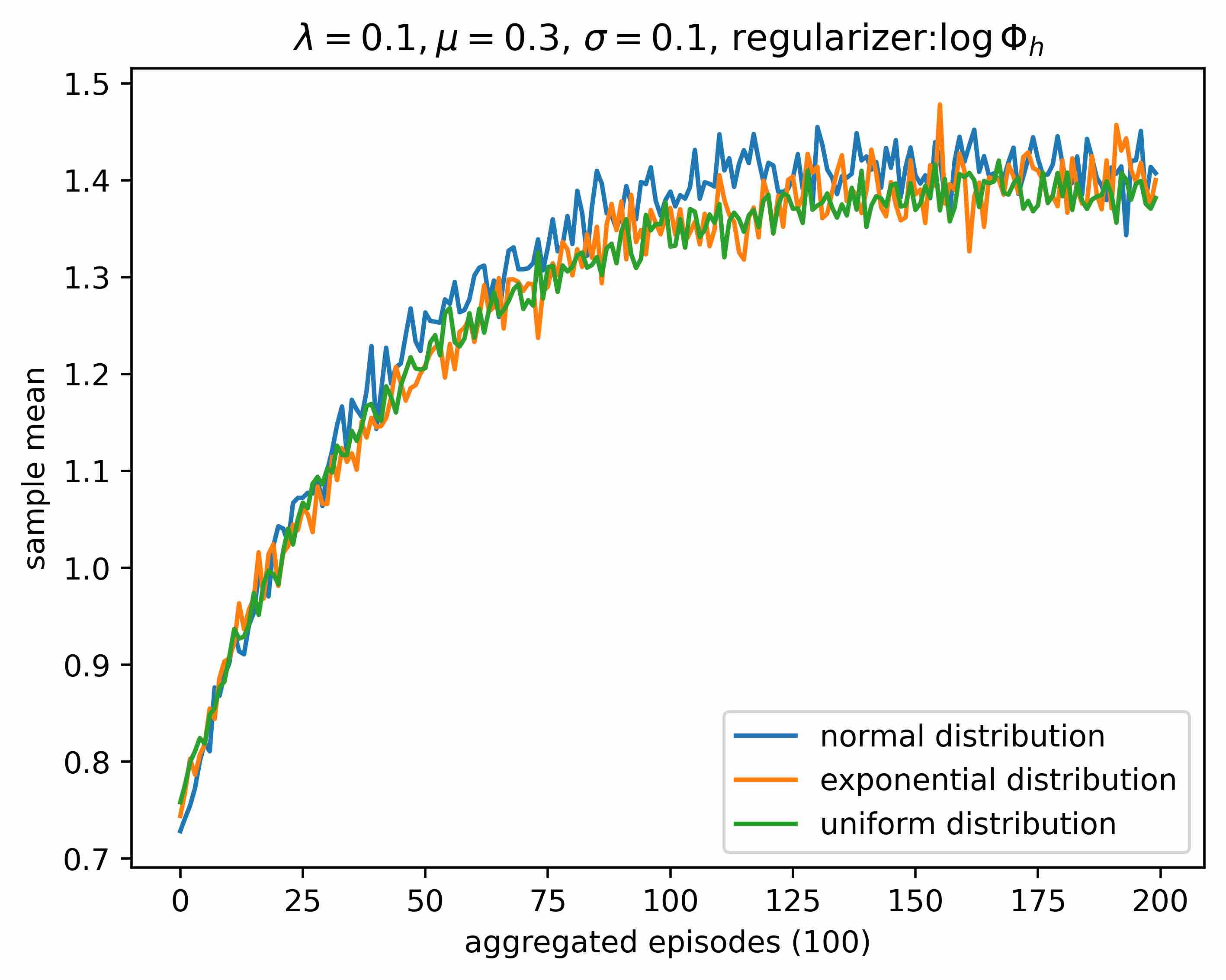
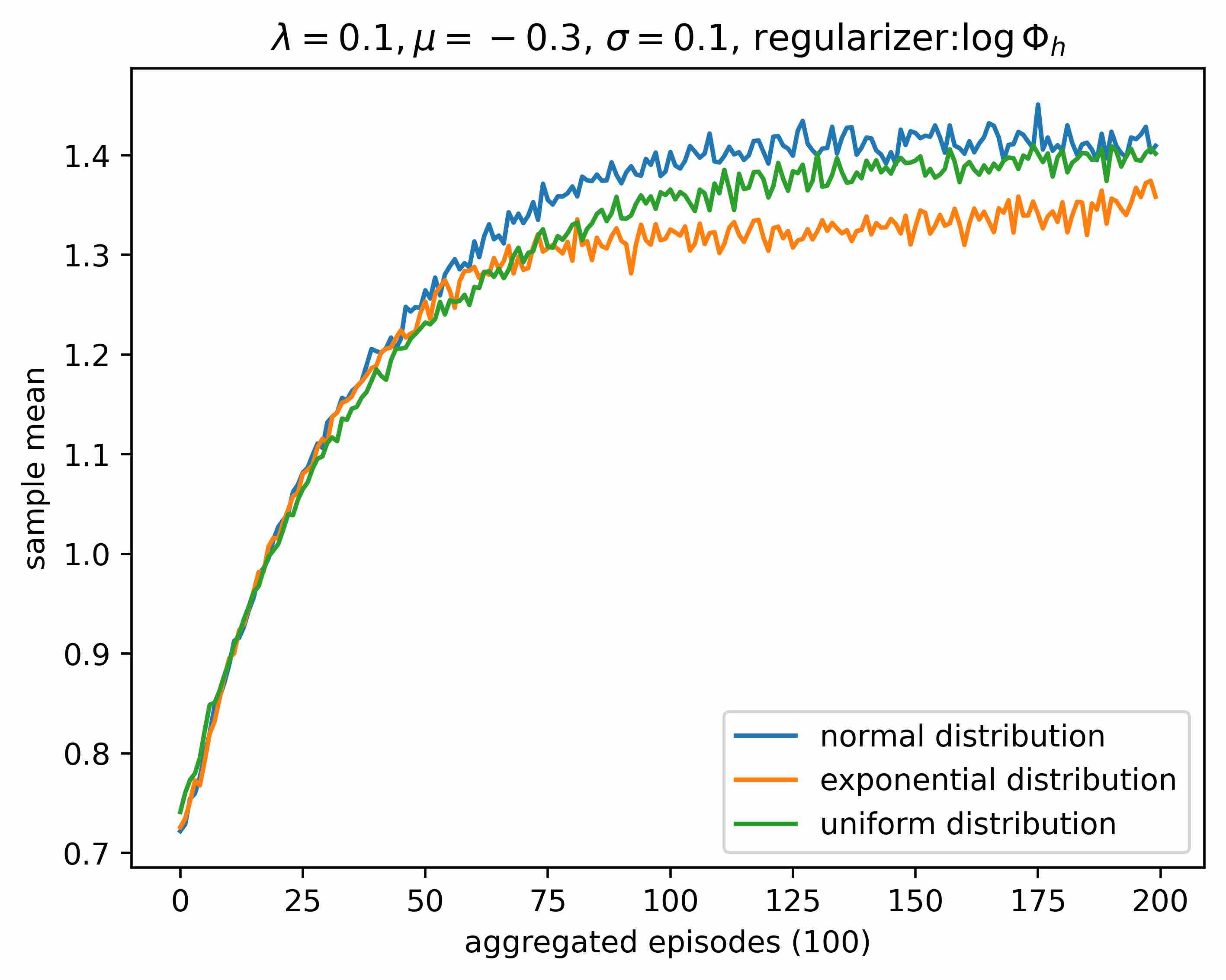
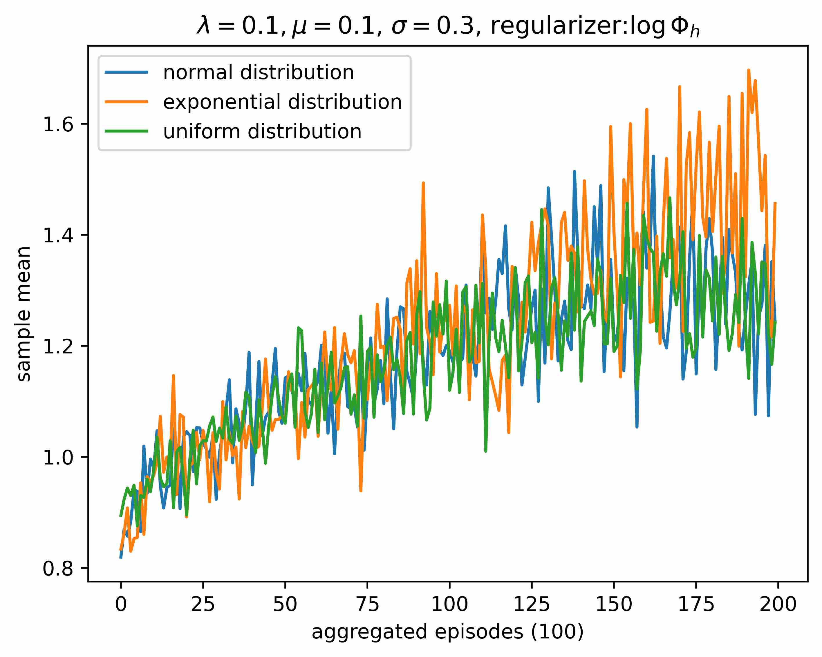
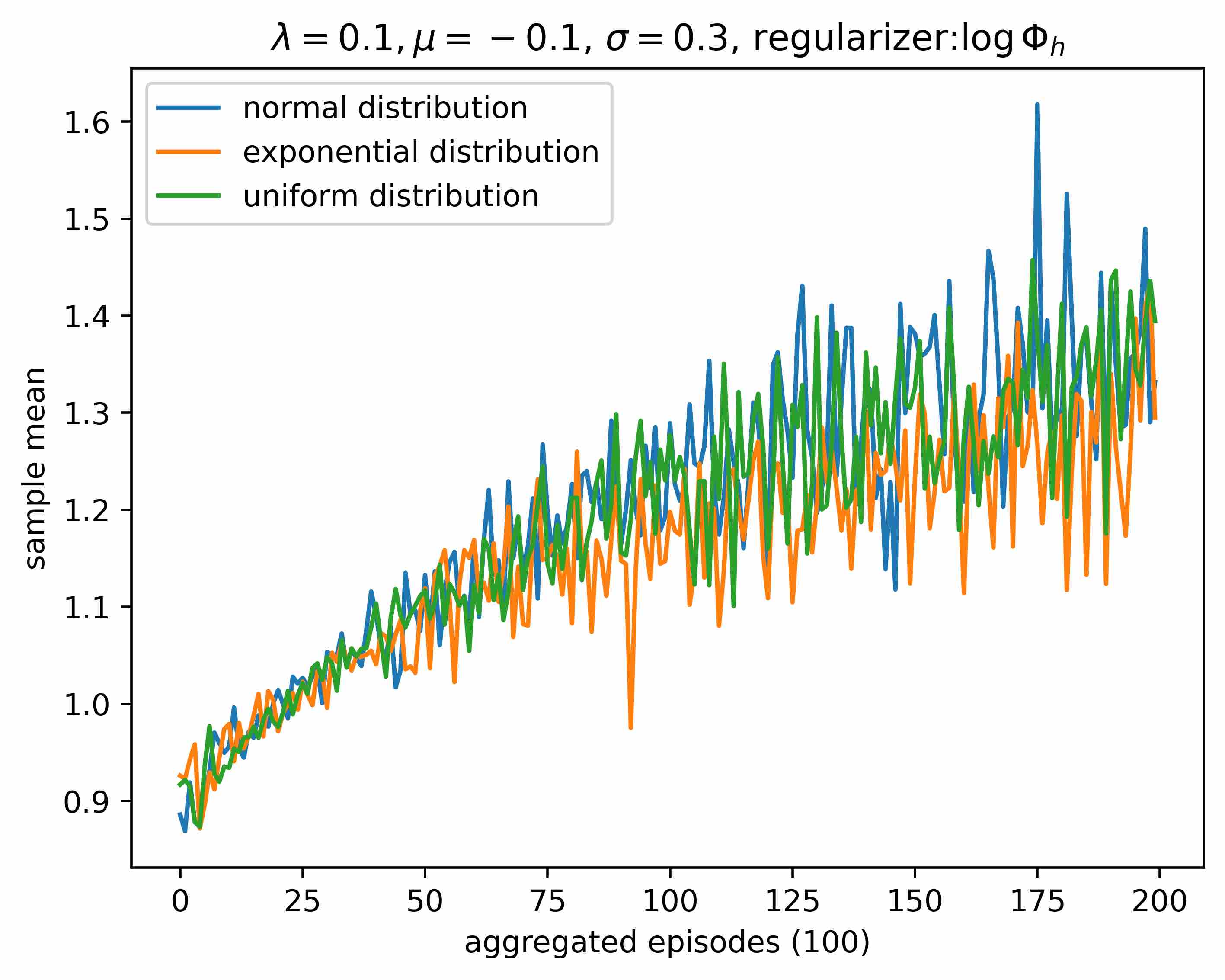
Figure 1: The effect of $\mu$ and $\sigma$ on the exploration for the regularizer $\log\Phi_{h}$

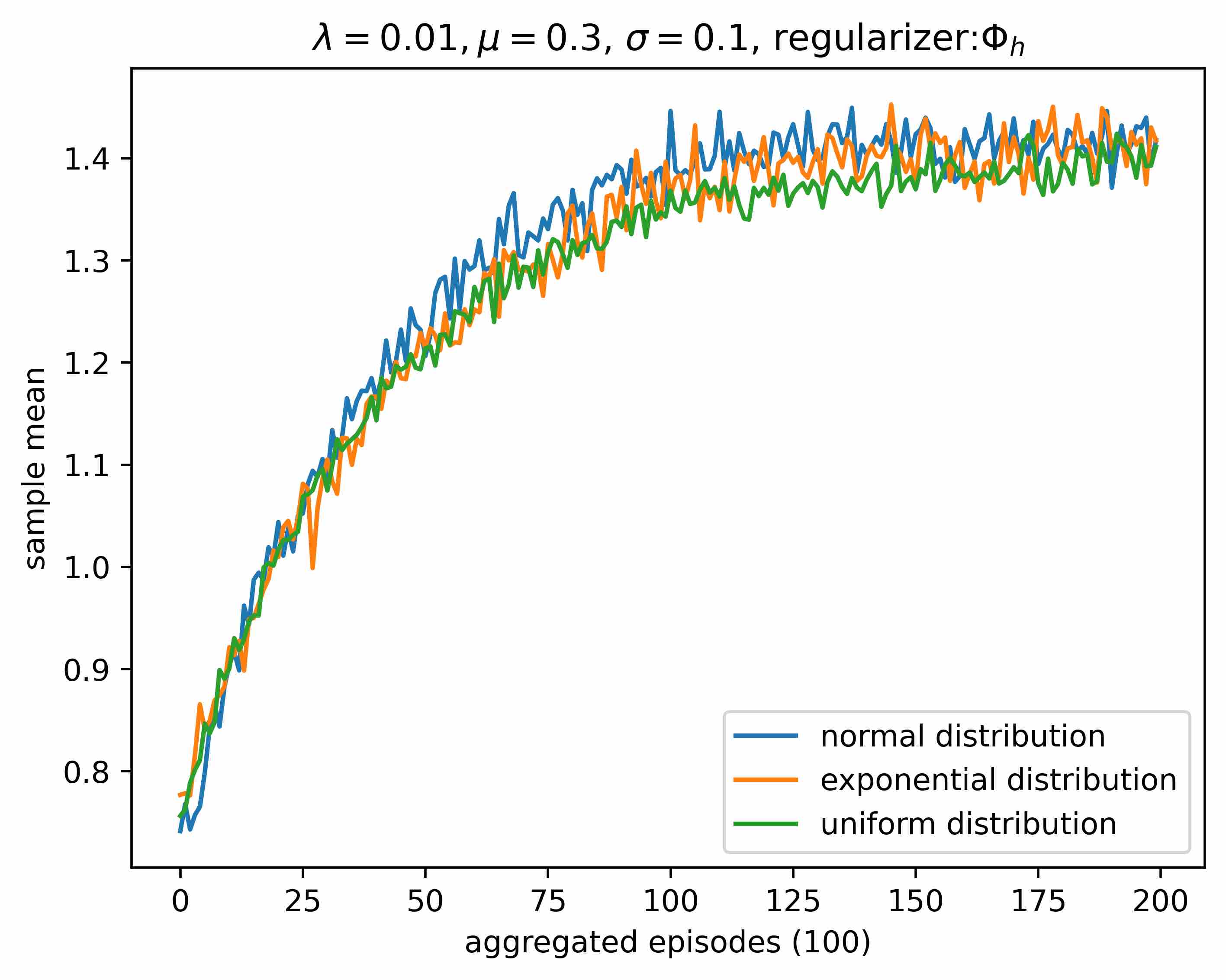
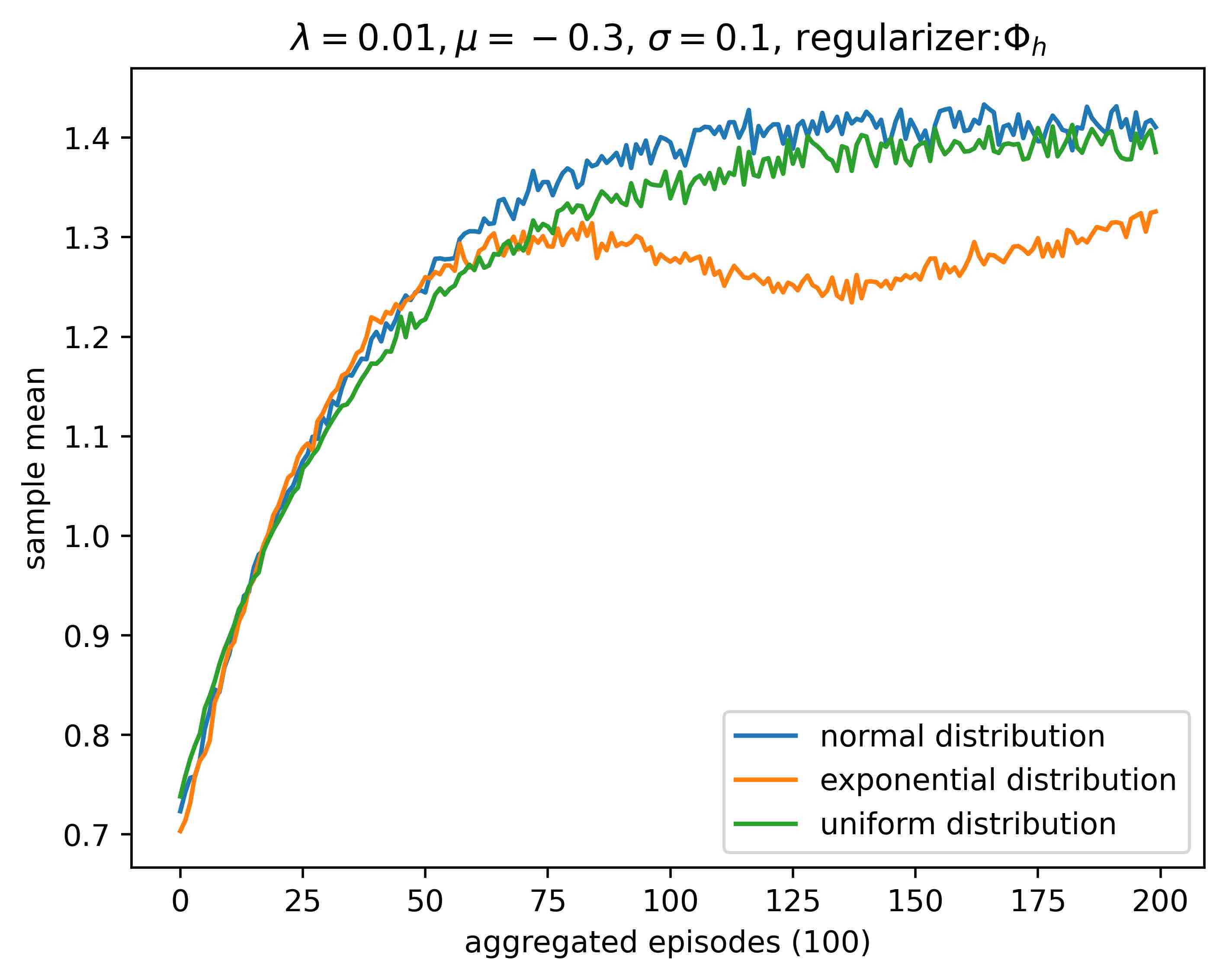
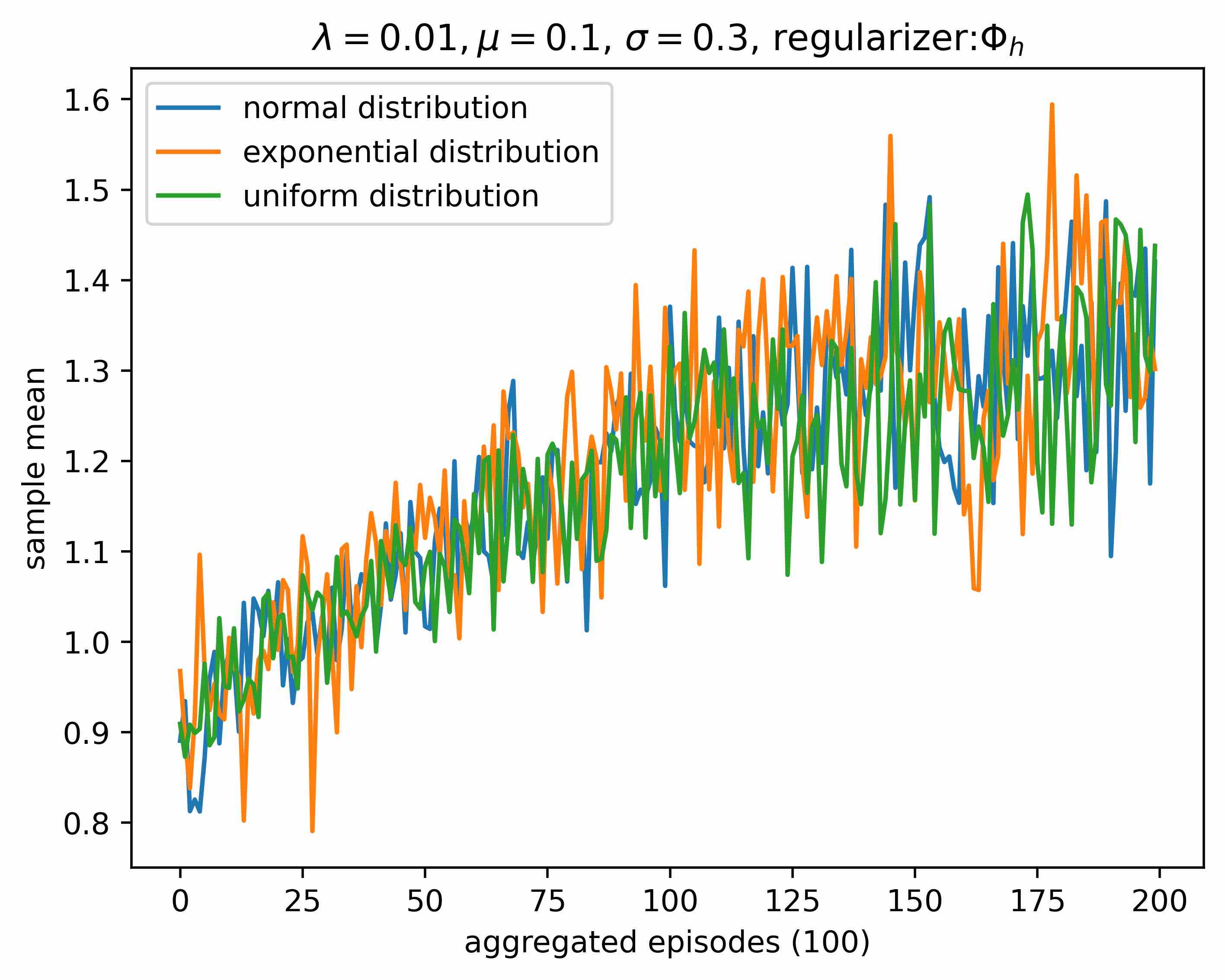
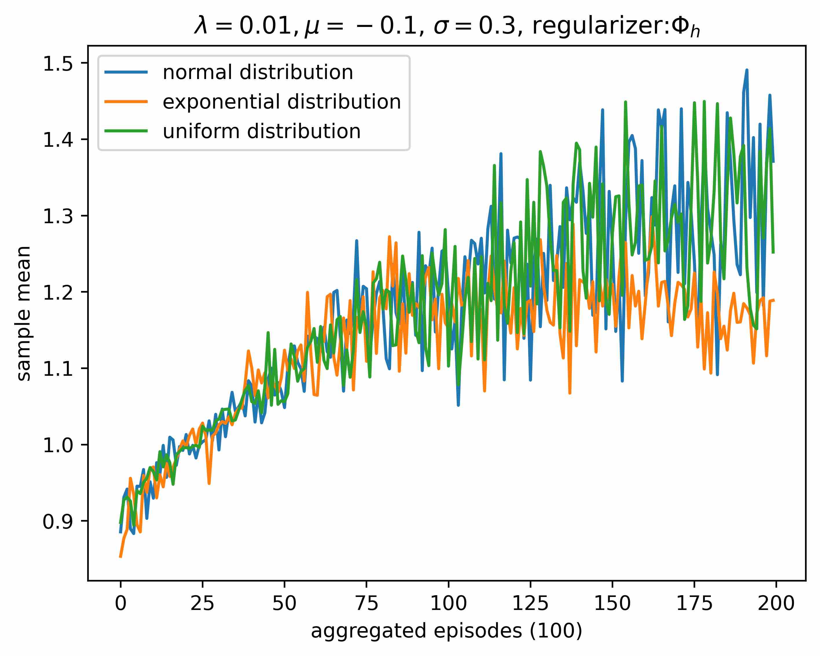
Figure 2: The effect of $\mu$ and $\sigma$ on the exploration for the regularizer $\Phi_{h}$

Figure 3: The effect of $\lambda$ on the exploration for the regularizer $\log\Phi_{h}$

Figure 4: The effect of $\lambda$ on the exploration for the regularizer $\Phi_{h}$

Figure 5: Samples of $u_{t_{i}}$ for the regularizer $\log\Phi_{h}$ and $\Phi_{h}$

7 CONCLUSION

For the first time, we applied the Choquet-regularized continuous-time RL framework proposed by Han et al. (2023) to practical problems. We studied the MV problem under Choquet regularization and its logarithmic form. Several different optimal exploration distributions of different $h$ were given, and when $\|h^{\prime}\|_{2}$ is fixed, the optimal exploration distributions have the same mean and variance. Unlike the infinite time horizon results in Han et al. (2023), the variance decreases over time in the finite time horizon problem. At the same time, the mean of the optimal exploration distribution is related to the current state $x$ and independent of $\lambda$ and $h$, which is equal to the optimal action of the classical MV problem. The variance of the optimal exploration distribution is related to $\lambda$ and $h$ and independent of state $x$, and even independent of $h$ under logarithmic regularization. These also showed the perfect separation between exploitation and exploration in the mean and variance of the optimal distributions as in Wang and Zhou (2020) when entropy is used as a regularizer.

Further, we have obtained that the two regularization problems converge to the traditional MV problem, and compared the exploration costs of the two regularizations. We found that the exploration cost under the logarithmic Choquet regularization is consistent with the exploration cost under the entropy regularization, only related to $\lambda$ and time range $T$, while the exploration cost under Choquet regularization is also related to market parameters. Through simulation, we compared the two kinds of regularization. In general, when the market fluctuates greatly and the willingness to explore is not strong, the cost of Choquet regularization is lower. On the contrary, it may be better to use logarithmic Choquet regularizers for regularization.

There are still some open questions. First of all, we regard $\lambda$ as an exogenous variable. From the perspective of exploration cost, turning $\lambda$ into endogenous and changeable can help us better control the exploration cost. As time goes by, the information we obtain through exploration will also increase, so the willingness to explore will also change, which also implies the rationality of the changing $\lambda$ to time-related. Secondly, the current Choquet integral can only deal with one-dimensional action space, thus how to extend the Choquet regularizers to multi-dimensional situations to adapt to more problems is still a challenging problem. We will study these issues in the future.

Acknowledgements.  This work was supported by the National Natural Science Foundation of China (No. 11931018 and 12271274)

References

- Dai et al. (2023) Dai, M., Dong, Y. and Jia, Y. (2023). Learning equilibrium mean-variance strategy. Mathematical Finance. doi.org/10.1111/mafi.12402.
- Doya (2000) Doya, K. (2000). Reinforcement learning in continuous time and space. Neural Computation, 12(1), 219–245.
- Gilboa and Schmeidler (1989) Gilboa, I. and Schmeidler, D. (1989). Maxmin expected utility with non-unique prior. Journal of Mathematical Economics, 18(2), 141–153.
- Gu et al. (2016) Gu, S., Lillicrap, T., Ghahramani, Z., Turner, R. E. and Levine, S. (2016). Q-prop: Sample-efficient policy gradient with an off-policy critic. arXiv: 1611.02247.
- Guo et al. (2020) Guo, X., Xu, R. and Zariphopoulou, T. (2020). Entropy regularization for mean field games with learning. arXiv: 2010.00145.
- Haarnoja et al. (2017) Haarnoja, T., Tang, H., Abbeel, P. and Levine, S. (2017). Reinforcement learning with deep energy-based policies. In Proceedings of the 34th International Conference on Machine Learning, pages 1353–1361.
- Han et al. (2023) Han, X., Wang, R. and Zhou, X. Y. (2023). Choquet regularization for continuous-time reinforcement learning. SIAM Journal on Control and Optimization, forthcoming.
- Hu and Chen (2020) Hu, T. and Chen, O. (2020). On a family of coherent measures of variability. Insurance: Mathematics and Economics, 95, 173–182.
- Jia and Zhou (2022a) Jia, Y. and Zhou, X. Y. (2022a). Policy evaluation and temporal-difference learning in continuous time and space: A martingale approach. Journal of Machine Learning Research, 23(154), 1–55.
- Jia and Zhou (2022b) Jia, Y. and Zhou, X. Y. (2022b). Policy gradient and actor-critic learning in continuous time and space: Theory and algorithms. Journal of Machine Learning Research, 23(154), 1–55.
- Jiang et al. (2022) Jiang, R., Saunders, D. and Weng, C. (2022). The reinforcement learning Kelly strategy. Quantitative Finance, 22(8), 1445–1464.
- Konda and Tsitsiklis (1999) Konda, V. and Tsitsiklis, J. (2000). Actor-critic algorithms. In Advances in Neural Information Processing Systems, pages 1008–1004.
- Li and Ng (2000) Li, D. and Ng, W. L. (2000). Optimal dynamic portfolio selection: Multiperiod mean-variance formulation. Mathematical Finance, 10(3), 387–406.
- Li et al. (2002) Li, X., Zhou, X. Y. and Lim, A. E. (2002). Dynamic mean-variance portfolio selection with no-shorting constraints. SIAM Journal on Control and Optimization, 40(5), 1540–1555.
- Liu et al. (2020) Liu, F., Cai, J., Lemieux, C. and Wang, R. (2020). Convex risk functionals: Representation and applications. Insurance: Mathematics and Economics, 90, 66–79.
- Markowitz (1952) Markowitz, H. (1952). Portfolio selection. The Journal of Finance, 7(1), 77–91.
- Neu et al. (2017) Neu, G., Jonsson, A. and Gómez, V. (2017). A unified view of entropy-regularized markov decision processes. arXiv: 1705.07798.
- Pesenti et al. (2020) Pesenti, S., Wang, Q. and Wang R. (2020). Optimizing distortion risk metrics with distributional uncertainty. arXiv: 2011.04889.
- Quiggin (1982) Quiggin, J. (1982). A theory of anticipated utility. Journal of Economic Behavior and Organization, 3(4), 323–343.
- Rao et al. (2004) Rao, M., Chen, Y., Vemuri, B. C. and Wang, F. (2004). Cumulative residual entropy: A new measure of information. IEEE Transactions on Information Theory, 50, 1220–1228.
- Sutton and Barto (2018) Sutton, R. S. and Barto, A. G. (2018). Reinforcement learning:An introduction. Cambridge, MA: MIT Press.
- Sunoj and Sankaran (2012) Sunoj, S. M. and Sankaran, P. G. (2012). Quantile based entropy function. Statistics and Probability Letters, 82(6), 1049–1053.
- Wang et al. (2020a) Wang, H., Zariphopoulou, T. and Zhou, X. Y. (2020a). Reinforcement learning in continuous time and space: a stochastic control approach. Journal of Machine Learning Research, 21(1), 8145–8178.
- Wang and Zhou (2020) Wang, H. and Zhou, X. Y. (2020). Continuous-time mean-variance portfolio selection: A reinforcement learning framework. Mathematical Finance, 30(4), 1273–1308.
- Wang et al. (2020) Wang, R., Wei, Y. and Willmot, G. E. (2020b). Characterization, robustness and aggregation of signed Choquet integrals. Mathematics of Operations Research, 45(3), 993–1015.
- Ziebart (2010) Ziebart, B. D. (2010). Modeling purposeful adaptive behavior with the principle of maximum causal entropy. PhD thesis.
- Zhou (2021) Zhou, X. Y. (2021). Curse of optimality, and how do we break it. SSRN: 3845462.
- Zhou and Li (2000) Zhou, X. Y. and Li, D. (2000). Continuous-time mean-variance portfolio selection: A stochastic LQ framework. Applied Mathematics and Optimization, 42(4), 19–33.