Lecture Notes for the 2023 Condensed Matter Summer School:
Introduction to random unitary circuits and the measurement-induced entanglement phase transition
Abstract
There are several nice review articles about the physics of random unitary circuits and the measurement-induced entanglement phase transition, most notably these two: [reviewrandomquantumcircuits2022, reviewentanglementdynamicsinhybridquantumcircuits]. This document has only two advantages over those nice reviews: (1) it’s shorter, and (2) since this is not a real article, I am not bound by the usual conventions of scientific writing.
Look, a duck:
.
1 Entanglement entropy and random unitary circuits
What distinguishes quantum information from classical information is the possibility of quantum entanglement. Generating, manipulating, and exploiting entanglement is sort of the whole point of quantum information as a science.
But entanglement can be a confusing quantity to think about: it doesn’t correspond to any direct observable the way that, say, energy or electric charge do. So it can be tricky to answer basic statistical mechanical questions about quantum entanglement. Questions like:
-
•
How does entanglement grow or spread throughout a many body system with time?
-
•
What are the statistics of random fluctuations in entanglement?
These kinds of questions about dynamics are very natural in many settings in condensed matter physics. But applying them to quantum entanglement requires some effort to pose the questions properly. The random unitary circuit is one of the primary tools for posing and addressing these kinds of questions.
1.1 How do you quantify quantum entanglement?
The usual textbook definition of quantum entanglement is something like:
“Quantum entanglement is when the state of the system cannot be completely specified by specifying the state of all its components in isolation.”
Or, if the textbook is being more mathematical, it will say something like:
“Suppose that a quantum system contains two parts and . If the state of the system can be written as , where and are states of and separately, then there is no quantum entanglement between and . If cannot be written this way, then and are entangled.”
So, for example, if I have two spins and , then the state
| (1) |
is one with no entanglement between the two spins, since the state can be fully specified by saying that spin is in the state and spin is in the state .
On the other hand, the singlet state
| (2) |
is entangled, since this state cannot be described as (something for A) (something for B).
The annoying thing about this usual definition, though, is that it gives you the impression that entanglement is a kind of binary thing: that you either can or cannot write the wave function as a product. In other words, it gives you no ability to think quantitatively about the question how entangled are and ? So I personally prefer to think about entanglement in terms of measurement outcomes, and to what degree making measurements on part B will affect the subsequent likelihood of getting different measurement outcomes for A.
Notice, for example, that if I have the state written above and I measure the value of spin B, then I will have two equally-likely outcomes: or . If I subsequently measure the state of spin A, after collapsing the state of spin B, then I will also have two equally likely outcomes. But the same would have been true if I had never done any measurements of spin B. So measuring the state of spin B does not at all affect how likely I am to get different measurement outcomes for A. Thus I can conclude that A and B are unentangled.
Contrast this with what happens for the singlet state . If I first measure B, then I can get one of two equally likely outcomes: or . Let’s suppose I measure B to be . Once I make this measurement for B, then I collapse the wave function to be . A subsequent measurement of spin A will definitely yield ; there is no longer any uncertainty about what the measurement will give. In other words, by first measuring B, I have reduced (in this case, entirely) the statistical entropy of the measurement outcomes of A.
This is the basic idea behind the quantity called the entanglement entropy . It quantifies the degree to which the statistical entropy of measurement outcomes for A is reduced by first completely measuring the state of B. To define , we first construct the density matrix . For a pure state ,
| (3) |
(In these lecture notes I will mostly be describing pure states, which are described by a wave function, as opposed to “mixed states”, which are a statistical sum of different wave functions.) I can define the “reduced density matrix” for A, , by doing a partial trace over values of B:
| (4) |
The “partial trace” means partitioning the density matrix into sectors according to the value of , and the doing the matrix trace within each sector. So, for example, the density matrix for the singlet state is
| (5) |
where the four rows/columns correspond to , , , and . The partial trace corresponds to doing a trace (sum of the diagonal) across the sub-matrices in each corner. This procedure gives
| (6) |
Notice that this is not something that could have been written as the outer product of any wave function with itself – it cannot represent any kind of pure state. Instead, it looks like a statistical mixture: 50% and 50% . The statistical entropy in this reduced density matrix tells you how entangled A is with B. (A quantum pure state always has zero statistical entropy – it is in a specific quantum state, rather than a probabilistic mixture of different states.)
So now we define the entanglement entropy as
| (7) |
The right-hand side should remind you of the Shannon entropy of a probability distribution
| (8) |
where labels different states. Taking the log of a matrix can be confusing, so it is often best to think about Eq. 7 in terms of the eigenvalues of the reduced density matrix :
| (9) |
(It is a general properties of density matrices that they are diagonalizable and have eigenvalues that sum to 1, , since the diagonal elements of the density matrix correspond to the probability of getting a particular measurement outcome.)
As it turns out, there is an entire family of similar measures of entropy called the “Renyi entropies” . These are all similar, but involve raising the probabilities to different powers . Specifically,
| (10) |
These Renyi entropies are not usually very different from each other conceptually, so it’s not typically worth making a big deal about the distinction between different values of . But it’s worth singling out three cases: , , and .
The limit of Eq. 10 has to be taken carefully, but if you do you’ll get Eq. 7, which is usually called the “von Neumann entanglement entropy”. It is perhaps the most common measure of entanglement entropy.
In the limit , any nonzero eigenvalue of becomes raised to the th power and thus becomes equal to , so we can write
| (11) |
gets called the “Hartley entropy” or “zeroth Renyi entropy”.
is a kind of stupid quantity in the sense that it changes discontinuously after an infinitessimal interaction. Imagine, for example, two unentangled spins. If I bring them together and allow them to interact for a very short time, I might expect that any entanglement between them will be very small. But jumps immediately from to , and in that sense is kind of a binary quantity that distinguishes only between “some entanglement” and “no entanglement” (I make this statement a bit more precise in the next subsection). All other with increase infinitesimally as you would expect. But, as we’ll see below, the Hartley entropy is useful in that it can usually be thought about in a straightforward classical way. Notice also that
| (12) |
That is, provides an upper bound for all the other ’s.
In the limit , the sum in Eq. 10 is dominated by the single largest eigenvalue , and so
| (13) |
The nice thing about is that it provides both an upper and lower bound for all other ’s with . It turns out that [wilming_entanglement_2019]
| (14) |
So, for example, if some with diverges, then all other with also diverge; and if some with remains small then so do all the others. So we often talk about a “generic” behavior of corresponding to . In principle Eq. 14 says nothing about , but in all cases that I know of behaves similarly to the “generic” case. By contrast, there are no guarantees that will behave in the “generic” way.
1.2 The Schmidt decomposition
There is a useful and general way to represent an entangled state called the Schmidt decomposition. The idea is that for any quantum state on subsystems A and B there is some set of orthonormal states and such that can be written
| (15) |
for some coefficients .
Notice that there are in general multiple ways to write a state as a sum over terms like . For example, the state that we looked at on page 1 could be written in a smart way as a sum with only one term (choosing the states and as in the first equality of Eq. 1); or it could be written in a dumb way as a sum over four terms: , , , and .
The Schmidt decomposition generally refers to the smartest way to do things, with the minimal number of terms in the sum. In fact, in this optimally compact decomposition the coefficients are the square root of the eigenvalues of the reduced density matrix .
One implication is that the zeroth Renyi entropy is exactly given by the (log of the) number of terms in the Schmidt decomposition:
| (16) |
That is, counts the minimal number of terms that you need in order to write a decomposition of the form of Eq. 15 if you want to represent the state exactly. But remember that the Schmidt decomposition is the smart way to write a state, and there are generally many dumb decompositions with more terms. So a corollary of Eq. 16 is
| (17) |
This last equation will be important when we discuss the idea of the minimal cut in Sec. 1.4.
1.3 The unitary circuit and the random unitary operator
1.3.1 The unitary circuit
A “unitary circuit” is a way of describing the evolution of a quantum state in discrete time rather than continuous time. In a unitary circuit, the quantum state evolves through the application of discrete operators to the quantum state (see Fig. 1).

There are multiple reasons why you might want to describe time evolution with a quantum circuit, rather than through a continuous-time evolution operator like . For example, maybe you are trying to describe a quantum computer, which operates using discrete quantum gates. Or maybe you really do care about a system with a continuous-time Hamiltonian, but for reasons of numerical or conceptual convenience you would like to approximate the dynamics by a sequence of discrete operators. For example, the picture on the right of Fig. 1 could serve as an approximation of a 1D spin chain with nearest-neighbor interactions.
Actually, there is a general theorem (often called the Lie-Trotter formula) that guarantees the validity of approximating any continuous time Hamiltonian via a sequence of discrete operators. Suppose I have a Hamiltonian that is a sum of many short-ranged parts , such that . In general the time evolution operator cannot be written as a simple product of separate operators for each . I mean that
| (18) |
Sadly, that’s not how matrix multiplication works. But the above expression becomes almost correct if the time interval of the evolution is very short. That is:
| (19) |
In other words, the time evolution of the full, many-body system can always be approximated by a product of many local operators , so long as I divide up the total time evolution into many small increments . Since the error from this approximation in a single step grows like , the total error from a long time evolution is still of order . So the dynamics of any many-body quantum system can be “Trotterized” into a quantum circuit, so long as you have the patience to put enough layers of operators in your circuit. And some circuit like the one on the right side of Fig. 1 starts to look like a universal approximation of a system with nearest-neighbor interactions.
1.3.2 Aside: who cares about random dynamics?
For people interested in the statistical mechanics of quantum entanglement growth, a big point of emphasis is the random unitary circuit. A random circuit is one for which either the structure of operators in time in space, or the operators themselves, are chosen in some random way. The very notion of “random dynamics” can seem a bit perverse – after all, no one operating a quantum computer or trying to figure out the ground state of a many-body Hamiltonian is thinking about random dynamics. And when the dynamics is random in time, it means that there is no concept of a Hamiltonian and no concept of energy: one cannot talk about “ground states” or “excited states.”
But there are reasons why one might want to think about random dynamics nonetheless. First, there is the hope that entanglement dynamics under a random circuit will be generic in some way. Just as the properties of random matrices end up being useful descriptors of a whole category of Hamiltonians, we can hope that by abstracting away from any specific Hamiltonian to a random quantum circuit we can uncover features of entanglement dynamics that are generic to a broad class of situations. Then, of course, specific situations might be “non-generic” in a variety of different ways – most likely, by introducing some conserved quantity (the total value of , for example). For the random dynamics considered in these lecture notes, it’s important that there are no conserved quantities.
Part of the motivation for studying entanglement dynamics in this way comes from the physics of thermalization. The question of thermalization concerns whether a quantum system that is completely isolated from its environment will be able to “act as its own bath”, such that quantities like charge, energy, etc. will be able to diffuse around and fill space in the usual way. One of our primary perspectives on thermalization is the Eigenstate Thermalization Hypothesis (ETH), which can be stated as follows. Consider a very large system, which we will divide into a macroscopic subsystem A and its (macroscopic) complement B. Suppose that the entire system is in an energy eigenstate with energy . One can associate a temperature with this eigenstate by saying that one would get the same energy (in expectation value) from a classical Boltzmann distribution if the temperature had a specific value . Such a classical Boltzmann distribution has a corresponding density matrix that is boring and classical: its diagonal entries are proportional to , where is the energy of the eigenstate , and the off-diagonal entries of are all zero. The ETH asserts that, if the energy eigenstate is “thermalized”, then the reduced density matrix for the subsystem A satisfies111The last equality in Eq. 20 makes use of the large system size limit – in general the off-diagonal components of the reduced density matrix are not literally zero under ETH, and there are interesting things to be said about them. But they are much smaller in magnitude than the diagonal components when A and its complement are both large.
| (20) |
In other words, tracing out everything outside of the region A leaves you with something that looks like the usual classical thermodynamics. (See [Nandkishore2015, deutsch_eigenstate_2018] for reviews of ETH.)
But this statement of ETH can only be satisfied if the subsystem A has extensive entanglement with its environment, since an equilibrium distribution at finite temperature has extensive entropy. We know of many systems that satisfy ETH (and in some sense satisfying ETH is the norm; we tend to find violations of ETH more interesting). So the question of how a system thermalizes – how it goes from something with little entanglement to something with a sufficiently extensive entanglement to satisfy ETH – is a question about entanglement dynamics. The random unitary circuit provides us with a tool to study some kind of “generic entanglement dynamics”, where entanglement forms more or less as quickly as allowed by spatial locality. Of course, in some particular situation this generic dynamics may or may not be stymied by the formation of some conserved quantity that bottlenecks the growth of entanglement.
Studying how quickly entanglement grows (or doesn’t) can be important for another more pragmatic reason. Until quantum computers become as good as Michio Kaku imagines them to be, simulating quantum systems is difficult computationally. And the more entangled the system is, the harder it is to simulate. Quantum states with only short-range entanglement have an efficient classical representation (say, in terms of matrix product states), but states with extensive entanglement do not. So knowing whether or not your state is going to develop extensive quantum entanglement becomes crucial for knowing whether your code is going to finish running in time for you to graduate.
1.3.3 Random unitary operators
The most generic type of random unitary operator is what’s called a “Haar-random” matrix. A Haar-random matrix is one that is chosen uniformly at random from the space of all possible unitary matrices.
Haar-random matrices are in some sense the “most random” operators possible, so they have been a major point of study. But they have the drawback that they necessarily produce dynamics that is hard to simulate classically: over time any nice and easily-written product state will spread to fill the full -sized Hilbert space (say, of qubits222Throughout these notes I’m going to use the words “spin” and “qubit” interchangeably. Sorry.), so that even storing the wave function becomes difficult computationally.
For that reason a common alternative is to instead consider only a more limited set of operators called Clifford operators. Clifford operators have the advantage that they shift the quantum state around within a limited subset of the Hilbert space, such that the state always has a compact classical representation (called a “codeword”). (See Sec. 3.3.4 of Ref. [reviewrandomquantumcircuits2022] for a nice and short overview of the Clifford group.) In this sense Clifford dynamics is “less random”, but it allows one to simulate large system sizes ( qubits) and long times on ordinary computers, while Haar-random dynamics is usually limited to only a couple dozen qubits.
1.4 The minimal cut: a classical bound on entanglement
Quantum mechanics is hard [18-19,654]. For that reason, much of the important progress in the field of entanglement dynamics has proceeded by finding clever analogies or mappings to classical problems. One of the cleverest and most central of these ideas (mostly developed in Ref. [Nahum_Quantum_2017]) is what’s called the “minimal cut”. The minimal cut is the most prominent recurring theme of these lecture notes.
1.4.1 Heuristic argument for the minimal cut
To understand, at a gut level, the minimal cut idea, imagine a circuit that looks like this:
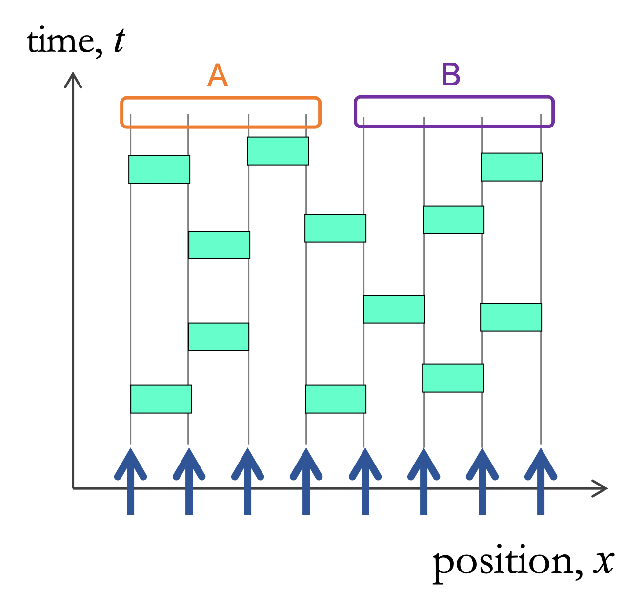
This circuit can be viewed as a kind of machine (formally, a tensor network) that takes a given input state to a corresponding output state.
Now suppose I want to estimate the entanglement entropy between the left half of my system and the right half (labeled A and B above) at the final time. I can, arbitrarily, draw a red line that divides this one tensor network into two smaller tensor networks, one whose output contains the state of the A qubits at the final time, and another whose output contains the state of the B qubits at the final time. Like so, perhaps:
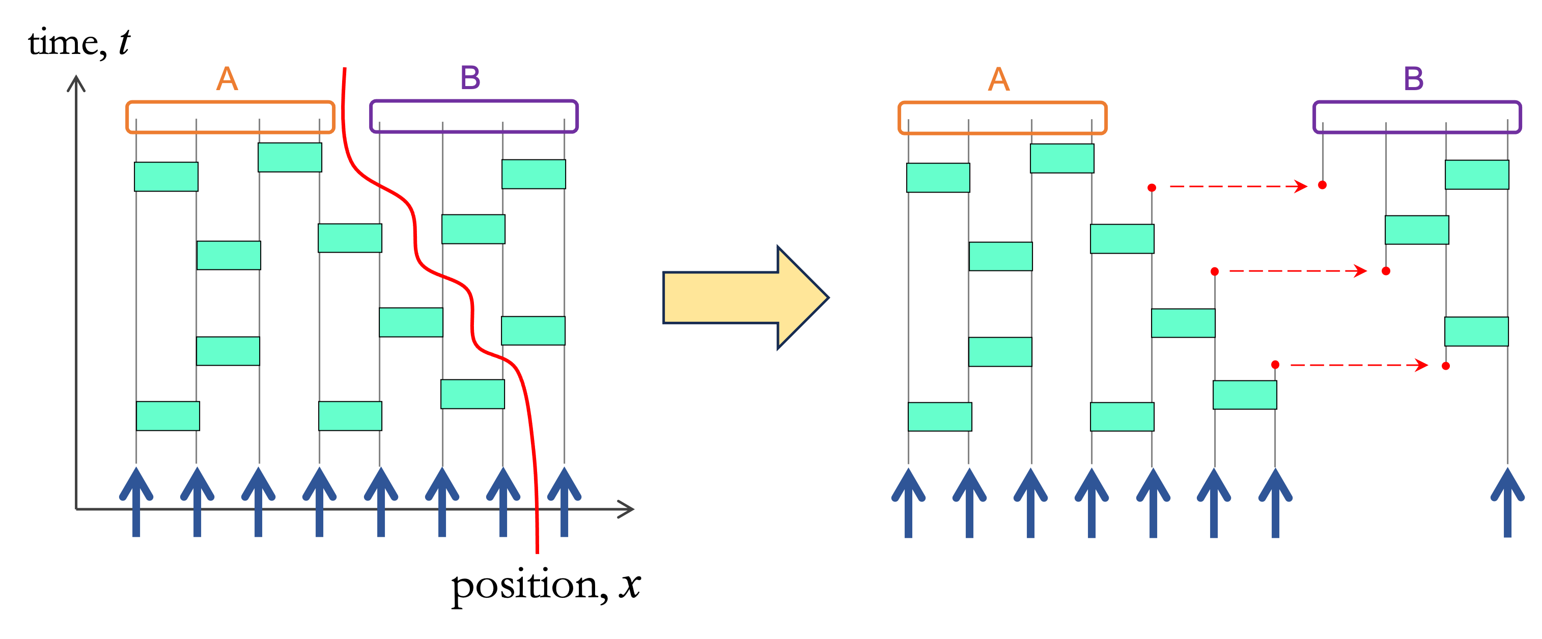
But by making this partition I have also created additional inputs and outputs for the two tensor networks. Here, the states of the qubits highlighted in red are outputs of the left tensor network that are used as inputs for the right tensor network. Each of these red circles can transmit at most one bit of information between the two tensor networks. In this example there are three shared connections between the two tensor networks, so consequently there can be at most three bits of information shared, which means that the entanglement entropy between A and B at the final time must be less than .
More generally, define as the number of legs of the circuit (black lines) that are severed when I draw a red line partitioning the tensor network into two pieces. (My line must always start at the top of the circuit at the midpoint between subsystems A and B, so that the output states of the two smaller tensor networks fully contain the subsystems A and B.) The quantity is equal to the number of shared connections between the two tensor networks. Since each connection can transmit at most one bit of information, I am generally guaranteed that for any
| (21) |
A more precise way to arrive at Eq. 21 is to realize that the partition shown in Fig. 3 actually represents a proposal for a way to write the final state as a decomposition. Let’s use to denote the operator defined by the left tensor network; in this example takes an input state with 7 spins to a state of 7 other spins (four that belong to A and three others that will be fed as inputs to the right tensor network). Meanwhile, the right tensor network is an operator that takes the state of four spins (three outputs from the left plus one from the initial time) to the four spins in B. Now notice that I can write the final state as
| (22) |
Here, the sum represents a sum over all possible states of the spins at the final time. And the sum is a sum over all possible states of the spins that are shared between the two tensor networks. The coefficients and represent the matrix elements of the operators and :
| (23) | ||||
| (24) |
There is nothing clever about Eq. 22; I am just summing directly over all possible output basis states of and , keeping in mind that the shared spins are the same. But notice that I can rearrange Eq. 22 slightly to get this:
| (25) |
Now you can see that I am proposing a way to write the state as a decomposition in the style of Eq. 15. The two quantities in the big parentheses represent state and that live only on the subsystems A and B. The number of terms in this proposed decomposition is the same as the number of possible states of the shared spins; so for this example my proposed decomposition has terms. Now you can recall Eq. 17, which tells me that my partition gives an upper bound on all the entropies:
| (26) |
Now comes the clever part. If you stare at Fig. 3 for a moment you’ll realize that there is a more frugal way to divide this circuit into two pieces. I mean that I could have drawn a partition that crosses fewer legs of the circuit. This partition involves only one shared connection:
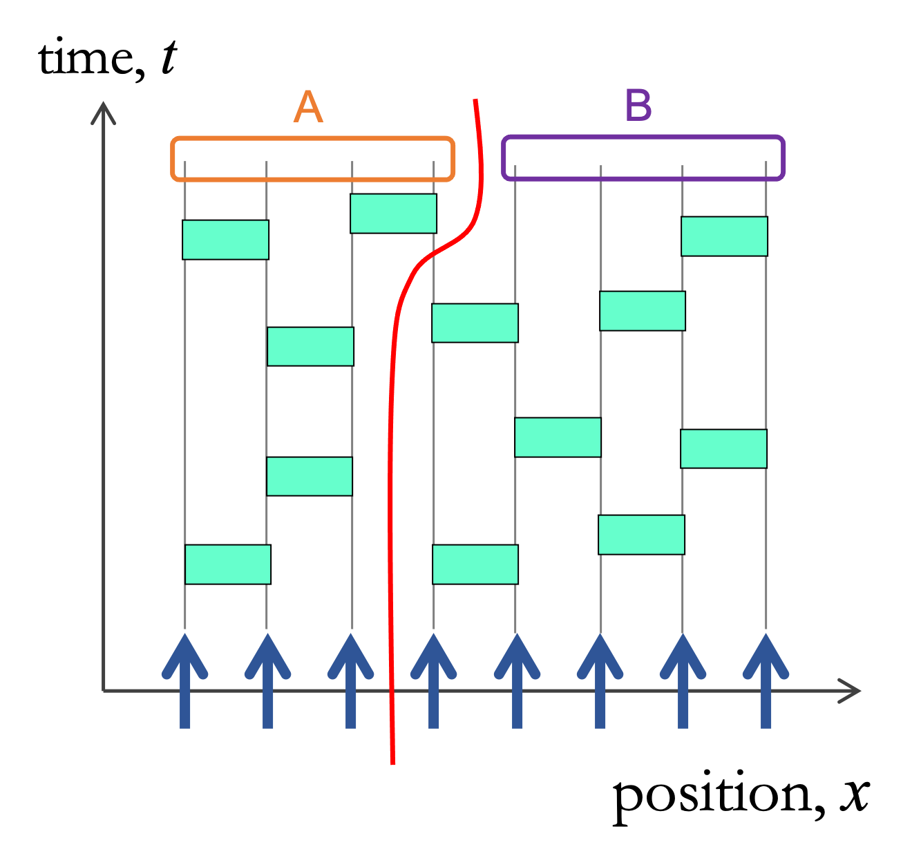
In fact, this choice represents the minimal cut. In this example there is no way to partition the network into two pieces that has a smaller number of cuts. So this minimal cut provides the tightest classical upper bound I can find on the entanglement:
| (27) |
Actually, for the case of random unitary operators, it happens that is exactly equal to .
In this way the behavior of is transformed into a classical problem about the geometry of the quantum circuit. One only need know the physical structure of the circuit to learn something about the entanglement entropy and how it changes with time (and with the way I choose to partition my system into subsystems A and B).
1.4.2 Universality class of entanglement growth and its fluctuations
Now that we have mapped the behavior of on to a classical geometry problem, we can look around to see whether someone smarter than ourselves has already solved that problem. In this case it turns out that they have. At long times and large system sizes, the minimal cut problem for a circuit with randomly-placed unitaries can be mapped onto a classical problem in statistical mechanics known as the directed polymer in a random environment (DPRE). In the DPRE problem, one imagines laying a continuous polymer down on a random energy landscape in such a way that the polymer’s energy is minimized. Here the “polymer” is the red line partitioning the circuit into two pieces and the “energy” is the value of , i.e. the number of circuit legs that are severed by the the minimal cut.
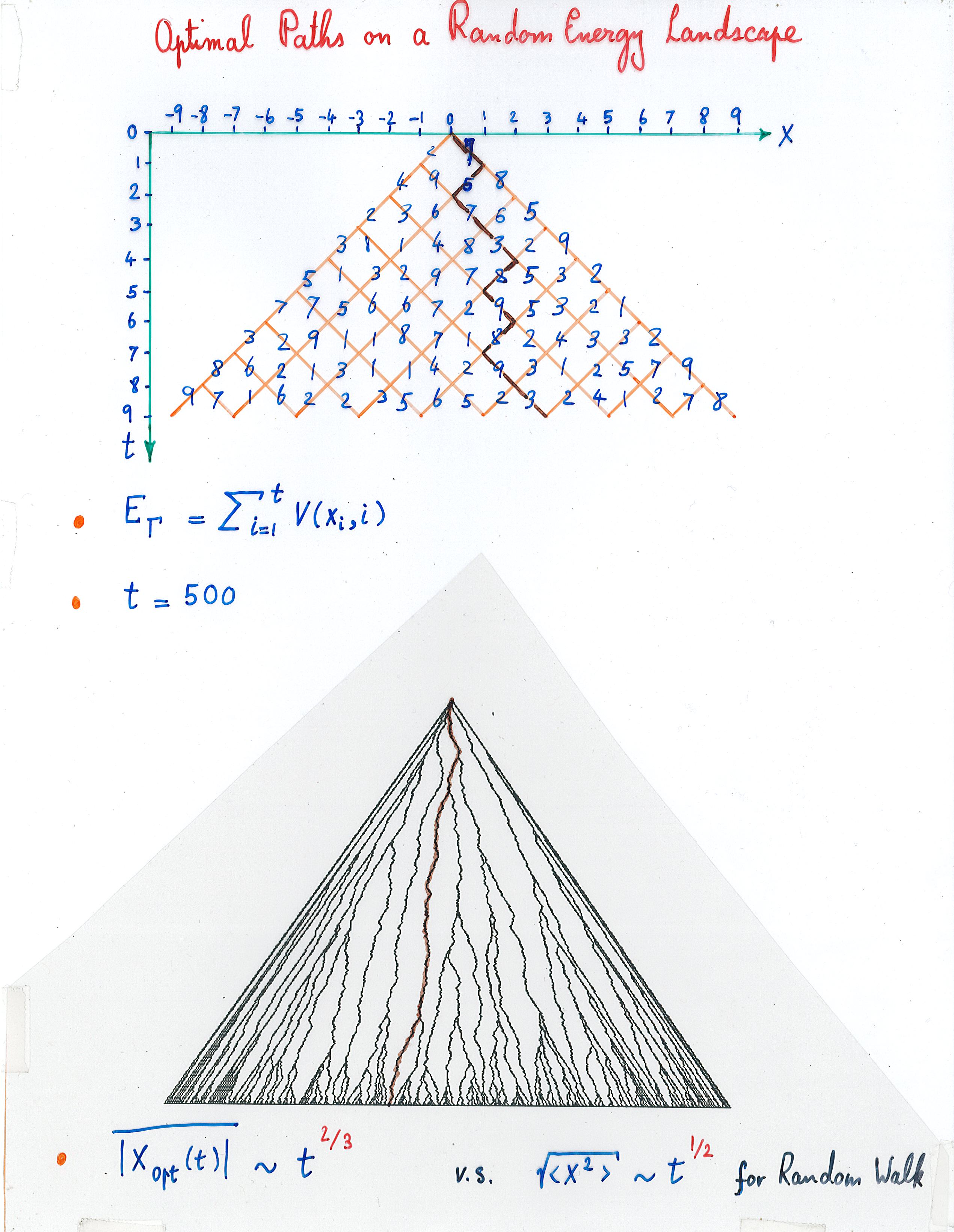
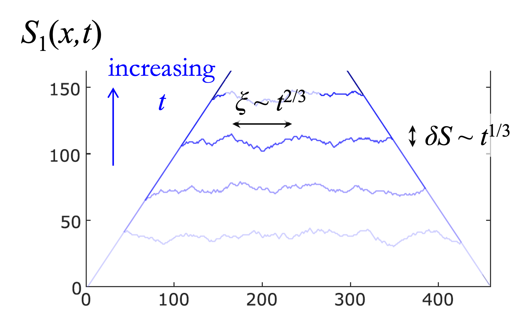
The beautiful thing about this analogy is that it allows one to figure out everything about the scaling and statistical fluctuations of the entanglement growth in a random circuit just by looking up the answers for the DPRE problem. As it happens, the DPRE problem belongs to the universality class of the Kardar-Parisi-Zhang (KPZ) equation.333The KPZ equation is commonly said to describe the evolution of the height of a randomly growing surface, like snow accumulating on a rooftop or the burning front of a piece of paper. It is generally written as , where describes random noise and the quantities , , and are parameters. From this mapping one can write down the scaling behaviors of the entanglement , where is the size of the left subregion (the distance from the left-hand side of the circuit to the point of separation between subsystems A and B) and is the evolution time. The primary results are:
-
1.
grows linearly in time at short times, and then saturates to a constant value for . (At such late times the minimal cut exits through the lateral boundary of the circuit, while for it exits through the bottom boundary.)
-
2.
Statistical fluctuations in grow with time as .
-
3.
Fluctuations in have a correlation length in space that grows as .
The realization that the dynamics of entanglement growth belongs to the KPZ universality class is surprisingly powerful. Once you’ve made this realization, you can look to any other system that belongs to the KPZ universality class and find a way to analogize it to the problem of quantum entanglement growth. In Ref. [Nahum_Quantum_2017], the authors point out three different and unexpected analogies to entanglement growth (in addition to DPRE, they make analogies to classical surface growth and to the asymmetric simple exclusion process, which is often used to model traffic jams). Each analogy brings some unexpected insight to the problem of entanglement growth in a random circuit.
1.5 The large- limit
I mentioned in 1.4.1 that the minimal cut generally provides a bound on , and that it exactly gives the zeroth Renyi entropy (Eq. 27). So the minimal cut generally gives an upper bound on the “generic” entanglement with . But there is no guarantee that will be particularly close to . It happens, though, that there is a particular limit where approaches exactly for all . This is the limit where each qubit in the system is replaced by a -state qudit and I allow the number of states . In this limit, all the Renyi entropies behave the same as the “classical” one .
There is a proof that at in Ref. [Nahum_Quantum_2017]. But a heuristic way to rationalize this result is as follows. Consider two spin- qudits A and B that are initially unentangled and are then acted on by a single random unitary matrix. This unitary matrix takes the two spins to an entangled state that can be described via a Schmidt decomposition (see Sec. 1.2)
| (28) |
The th Renyi entropy is
| (29) |
As long as the unitary matrix is random, then all of the Schmidt coefficients will be nonzero with probability 1, which means that the zeroth Renyi entropy . In principle, to calculate the other Renyi entropies we need to know the values of the ’s, which are random in some way, subject to the constraint that . But the key is that, when is large, nearly all random states have sets of such that most of the ’s are of the same order of magnitude . So in this large- limit we can estimate the sum
| (30) |
From Eq. 10 this gives exactly .
So the point is that, when is large, the very large Hilbert space of each qudit guarantees that just about any randomly chosen state is very close to being maximally entangled. So as long as we are using random operators we can be confident that all will approach the upper bound .
2 The measurement-induced entanglement phase transition
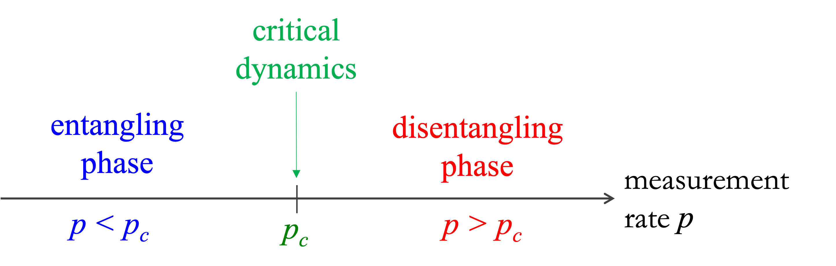
The idea of the measurement-induced entanglement phase transition (which I will shorten to just “measurement phase transition”, MPT) came from a very simple observation: unitary operators tend to increase the entanglement, while measurements tend to decrease it. For example, I can entangle two spins by applying a unitary operator to them, but if I measure the spin of either one I will disentangle them again. So what happens if I have a collection of many spins that is simultaneously being acted on by unitary operators and undergoing sporadic measurement? How is the competition between entangling forces (unitary operators) and disentangling forces (measurements) resolved? Do the unitary operators win so that the entanglement continues to grow with time? Or do the measurements win so that the entanglement growth is blocked?
The answer, perhaps surprisingly, is that there is a phase transition between these two possibilities as a function of the measurement rate. When measurements are made sufficiently infrequently, there is an “entangling phase”, in which entanglement grows and becomes extensive. When measurements are more frequent than a specific critical rate, however, the dynamics is “disentangling” and cannot support extensive entanglement.
There are different ways to characterize the entangling and disentangling phases (sometimes called the “weak monitoring” and “strong monitoring” phases). A general summary of the features of the two phases is like this:
-
Entangling phase:
-
–
Entanglement grows and becomes extensive.
Starting with a pure initial state having low entanglement, entanglement grows linearly in time and ultimately saturates at a value proportional to the subsystem size. -
–
An initially mixed state is basically never purified.
A highly mixed initial state remains highly mixed for a long time. Its mixedness decays to zero only over a time scale that is exponential in the system size.
-
–
-
Disentangling phase:
-
–
Entanglement is blocked from growing.
An initially pure state with low entanglement will never develop extensive quantum entanglement. The growth rate of entanglement goes to zero in an order-1 time scale. A highly entangled initial state will see its entanglement drop to a value of order-1. -
–
Initially mixed states are easily purified.
The mixedness of a highly-mixed initial state decays to zero over an order-1 time scale, even for large system sizes.
-
–
How best to understand the measurement phase transition (MPT) is largely still an open question. Just 5 years after the MPT was first suggested, there are now many contexts in which an MPT or something like it is known to appear. But in most of these contexts there is still no exact solution for the transition or its critical properties.
But since I was personally involved in one of the first papers to suggest the existence of the MPT (Ref. [Skinner_Measurement_2019], which was released simultaneously with Refs. [Li_Quantum_2018, Chan_Unitary-projective_2019] considering the same question), I can at least explain why we expected the MPT to exist.
2.1 The original problem in dimensions
The first context in which the MPT was identified is as follows. Consider a 1D line with spins/qubits that start out in a simple product state like and evolve via a brickwork circuit of unitary operators. We can imagine that all the operators are chosen Haar-randomly.555This choice of Haar-random matrices turns out to not matter. Using Clifford unitaries or even taking every brick to be the same unitary matrix44footnotemark: 4 gives qualitatively the same results for the MPT.