Vortex loop dynamics and dynamical quantum phase transitions in 3D fermion matter

Abstract

In this study, we investigate the behavior of vortex singularities in the phase of the Green’s function of a general non-interacting fermionic lattice model in three dimensions after an instantaneous quench. We find that the full set of vortices form one-dimensional dynamical objects, which we call vortex loops. The number of such vortex loops can be interpreted as a quantized order parameter that distinguishes between different non-equilibrium phases. We show that changes in this order parameter are related to dynamical quantum phase transitions (DQPTs). Our results are applicable to general lattice models in three dimensions. For concreteness, we present them in the context of a simple two-band Weyl semimetal. We also show that the vortex loops survive in weakly interacting systems. Finally, we observe that vortex loops can form complex dynamical patterns in momentum space due to the existence of band touching Weyl nodes. Our findings provide valuable insights for developing definitions of dynamical order parameters in non-equilibrium systems.

Introduction. Due to advancements in experimental technologies and a deeper theoretical understanding, the field of non-equilibrium quantum many-body dynamics has rapidly progressed in the recent decade Polkovnikov et al. (2011). This has led to the exploration of exciting, ergodicity-broken states and phases of quantum matter Mori et al. (2018); Moudgalya et al. (2022), such as many-body scars Abanin et al. (2019) and time crystals Khemani et al. (2019); Sacha (2020), which are of inherent non-equilibrium nature and go beyond standard thermodynamics and the theory of quantum phase transitions Sachdev (2000); Dziarmaga (2010). It has also been discovered that a non-equilibrium unitary evolution of quantum states can give rise to temporal non-analyticities in the rate of the Loschmidt amplitude, which is analogous to the singularities observed in thermodynamic functions during equilibrium phase transitions. This phenomenon, termed a dynamical quantum phase transition (DQPT) Heyl et al. (2013); Zvyagin (2016); Heyl (2018, 2019), has recently attracted a lot of attention from both theoretical Budich and Heyl (2016); Halimeh and Zauner-Stauber (2017); Žunkovič et al. (2018); Lang et al. (2018); Heyl et al. (2018); Kosior and Sacha (2018); Kosior et al. (2018); Yang et al. (2019); Zhou and Du (2021); Peotta et al. (2021); Trapin et al. (2021); Bandyopadhyay et al. (2021); Halimeh et al. (2021); De Nicola et al. (2021) and experimental Fläschner et al. (2017); Zhang et al. (2017); Guo et al. (2019); Tian et al. (2020); Jurcevic et al. (2017) communities (for related non-equilibrium transitions characterized by order parameters see Refs. Yuzbashyan et al. (2006); Sciolla and Biroli (2010); Halimeh et al. (2017); Marino et al. (2022)). While it has been demonstrated in different cases that DQPTs are directly linked to the equilibrium phase transition of the system being studied, this connection cannot be considered a one-to-one correspondence in general Vajna and Dóra (2014). Therefore, DQPT is expected to be a genuine non-equilibrium phenomenon without equilibrium counterpart. Remarkably, DQPTs for a non-interacting system in two dimensions (2D) can be closely related to the emergence of measurable, dynamical vortex-like singularities in the phase of the Green’s function in momentum space Yu (2017); Qiu et al. (2018); Lahiri and Bera (2019); Sim et al. (2022) (for experiments see Fläschner et al. (2017); Tarnowski et al. (2019)). It has been shown so far that the vortices appear as stable objects in 2D two-band models, but higher-dimensional systems have remained unexplored so far.

In the following we show that in three-dimensional (3D) models vortices of the Green’s function are not isolated, but they rather constitute one-dimensional (1D) dynamical objects, which we call vortex loops, the number of which can be interpreted as a quantized order parameter that distinguish between different non-equilibrium phases. We show that a change of a dynamical order parameter is always related to a DQPT, hence the critical points in time can be simply identified from the rate function of the Loschmidt amplitude. Although we stress that our findings are generic and applicable to a general fermionic translationally symmetric lattice model in 3D, for the sake of clarity the presentation of results is focused on a simple Weyl semimetal model with two bands Weyl (1929); Delplace et al. (2012); Xu et al. (2015); Chen et al. (2015); Armitage et al. (2018); Wang et al. (2021). Moreover, we show that the vortex loops are robust and survive in weakly interacting systems. Additionally, due to the existence of band touching Weyl nodes, we find that in a long time limit the loops can form complex dynamical patterns in momentum space.

General setup and observables. Before we turn to a specific microscopic model, we start this section with a very general picture. We consider a particle-hole symmetric model of non-interacting spin-$1/2$ fermions with translational invariance on a 3D lattice. The Hamiltonian of such a system can be written in a form:

$$\hat{H}=\sum\nolimits_{\mathbf{k}\in\textrm{BZ}}\hat{\psi}_{\mathbf{k}}^{\dagger}H_{\mathbf{k}}\hat{\psi}_{\mathbf{k}},\quad H_{\mathbf{k}}=\vec{h}_{\mathbf{k}}\cdot\vec{\sigma},$$ (1)

with the summation going over independent quasi-momenta $\mathbf{k}$ of a Brillouin zone (BZ). Here $\hat{\psi}_{\mathbf{k}}$ denotes a fermionic spinor operator, $\vec{\sigma}$ is a vector of Pauli matrices and $\vec{h}_{\mathbf{k}}$ is a vector defined by microscopic details of a particular model. Here, without a loss of generality, we consider $\hat{\psi}_{\mathbf{k}}^{\dagger}=[\hat{c}_{{\mathbf{k}},\uparrow}^{\dagger},\hat{c}_{{\mathbf{k}},\downarrow}^{\dagger}]$ with $\hat{c}_{{\mathbf{k}},\sigma={\uparrow,\downarrow}}^{\dagger}$ being standard creation operators foo (a), but we note that the precise form of $\hat{\psi}_{\mathbf{k}}$ might also be different depending on the choice of a two band model. Throughout this work we adopt a unit lattice spacing and set $\hbar=1$.

Furthermore, we assume that the system is prepared in a fermionic ground state at a half filling, namely, $|\psi_{0}\rangle=\Pi_{\mathbf{k}\in\mathrm{BZ}}|\mathbf{k}_{-}^{\mathrm{(i)}}\rangle$, where $|\mathbf{k}_{-}^{\mathrm{(i)}}\rangle=\hat{c}_{\mathbf{k}}^{\mathrm{(}i)\dagger}|0\rangle$ is the lower state of some initial Hamiltonian $H_{\mathbf{k}}^{\mathrm{(i)}}=\vec{h}^{\mathrm{(i)}}_{\mathbf{k}}\cdot\vec{\sigma}$, see foo (b). At a time $t=0$ we perform an instantaneous quench of at least one of the model’s parameters, which results in a sudden change of the Hamiltonian $\vec{h}^{\mathrm{(i)}}_{\mathbf{k}}\rightarrow\vec{h}^{(\mathrm{f})}_{\mathbf{k}}$. After the quench, the initial state $|\psi_{0}\rangle$ evolves under the new Hamiltonian $H_{\mathbf{k}}^{(\mathrm{f})}=\vec{h}^{(\mathrm{f})}_{\mathbf{k}}\cdot\vec{\sigma}$, i.e., $|\psi(t)\rangle=\Pi_{{\mathbf{k}}\in\mathrm{BZ}}|\mathbf{k}(t)\rangle$ with

$$|{\mathbf{k}}(t)\rangle=\sum_{\alpha=\pm}\Gamma_{\mathbf{k}}^{\alpha}e^{-i\epsilon_{\mathbf{k},\alpha}t}|\mathbf{k}_{\alpha}^{(\mathrm{f})}\rangle,\quad\Gamma_{\mathbf{k}}^{\alpha}=\langle\mathbf{k}_{\alpha}^{(\mathrm{f})}|\mathbf{k}_{-}^{\mathrm{(i)}}\rangle,$$ (2)

where $|\mathbf{k}_{\alpha}^{(\mathrm{f})}\rangle=\hat{c}_{\mathbf{k},\alpha}^{\textrm{(f)}\dagger}|0\rangle$ is an eigenvector of $H_{\mathbf{k}}^{(\mathrm{f})}$ with the corresponding eigenenergy $\epsilon_{\mathbf{k},\alpha=\pm}=\pm\epsilon_{\mathbf{k}}$. We assume that the quench preserves translational invariance so that a quasi-momentum ${\mathbf{k}}$ remains a good quantum number.

To investigate the dynamics of the non-equilibrium system we focus on the time ordered Green’s function Peskin (2018)

$$g_{\mathbf{k}}(t)=\sum_{\mathbf{r},\sigma}e^{i\mathbf{k}\cdot\mathbf{r}}\langle\hat{c}_{\mathbf{r},\sigma}(t)^{\dagger}\hat{c}_{\mathbf{r}=0,\sigma}\rangle=\sum_{\mathbf{q},\sigma}\langle\hat{c}^{\dagger}_{\mathbf{k},\sigma}(t)\hat{c}_{\mathbf{q},\sigma}\rangle,$$ (3)

where in the above we denote $\langle\ldots\rangle=\langle\psi_{0}|\ldots|\psi_{0}\rangle$ and $\hat{c}_{\mathbf{r},\sigma}=1/\sqrt{N}\sum_{\mathbf{k}}e^{-i\mathbf{k}\cdot\mathbf{r}}\hat{c}_{\mathbf{k},\sigma}$. Alternatively, one could also study the Loschmidt amplitude $\mathcal{G}(t)=\langle\psi_{0}|\psi(t)\rangle=\langle\psi_{0}|e^{-i\hat{H}^{\textrm{(f})}t}|\psi_{0}\rangle$, which quantifies how far the time evolution drives the system away from the initial condition. The Loschmidt amplitude can be conveniently written as $\mathcal{G}(t)=\Pi_{\mathbf{k}}\mathcal{G}_{\mathbf{k}}^{(1)}(t)$, with

$$\mathcal{G}_{\mathbf{k}}^{(1)}(t)=\langle 0|\hat{c}_{\mathbf{k}}^{\textrm{(i)}\dagger}(t)\hat{c}_{\mathbf{k}}^{\textrm{(i)}}|0\rangle=\langle\mathbf{k}_{-}^{\textrm{(i)}}|\mathbf{k}_{-}^{\textrm{(i)}}(t)\rangle.$$ (4)

Since the Loschmidt amplitude $\mathcal{G}$ for a many body system is a fast decaying function with the increasing number of particles $N$, it is convenient to define the rate function, $\lambda=-\lim_{N\rightarrow\infty}\ln|\mathcal{G}|^{2}/N$. The latter bears formal resemblance to the free energy density (with temperature replaced by time $t$) and, therefore, $\lambda$ might be viewed as a non-equilibrium free energy analog. This analogy implies that the rate function $\lambda$ can show signatures of a phase transition having non-analytic points that appear dynamically in time giving rise to a dynamical quantum phase transition (DQPT) Heyl et al. (2013); Zvyagin (2016); Heyl (2018, 2019). For the considered setup the rate function can be expressed analytically, i.e.,

$$\lambda(t)=-\int\frac{\mathrm{d}\mathbf{k}}{(2\pi)^{3}}\ln\left[1+\left[\big{(}\hat{h}_{\mathbf{k}}^{\mathrm{(}i)}\cdot\hat{h}_{\mathbf{k}}^{\mathrm{(}f)}\big{)}^{2}-1\right]\sin^{2}(\epsilon_{\mathbf{k}}t)\right],$$ (5)

with the normalised vectors $\hat{h}_{\mathbf{k}}=\vec{h}_{\mathbf{k}}/(\vec{h}_{\mathbf{k}}\cdot\vec{h}_{\mathbf{k}})^{1/2}$.

To ensure clarity, throughout the article we have chosen to focus on a single model while still drawing general conclusions. Specifically, we consider a two-band 3D Weyl semimetal Hamiltonian foo (c), given by

$$\vec{h}_{\mathbf{k}}=\left[\sin k_{x},\sin k_{y},m_{z}-\cos k_{z}\right],$$ (6)

and we assume a quench of the free parameter $m_{z}$ between two distinct topological phases: a normal insulator ($|m_{z}|>1$), and a Weyl semimetal ($|m_{z}|<1$) characterized by pairs of Weyl points and linear Dirac-like dispersion around them. As we will demonstrate, this quench induces a DQPT and leads to the appearance of 1D dynamical singularities in the phase of the Green’s function.

Relating DQPTs with phase singularities. For a non-interacting system, it can be shown that $\mathcal{G}_{\mathbf{k}}^{(1)}=\overline{g_{\mathbf{k}}}$, i.e., the Green’s function is a complex conjugate of the first order correlation function foo (d), which implies that a DQPT can be observed on a Green’s function level. Indeed, the non-analytic points of the rate function $\lambda(t)$ can only occur if and only if $g_{\mathbf{k}}(t)=|g_{\mathbf{k}}(t)|\exp[i\phi_{\mathbf{k}}(t)]$ vanishes for some $\mathbf{k}^{*}$ and $t^{*}$, implying a phase singularity of the Green’s function $\phi_{\mathbf{k}}(t)$ Heyl (2018). While in 1D systems the phase singularities can be only observed in a $k-t$ plane Budich and Heyl (2016); Zache et al. (2019), in 2D models these singularities appear as isolated dynamical point vortices with clockwise or anticlockwise phase winding Yu (2017); Qiu et al. (2018); Lahiri and Bera (2019); Sim et al. (2022) (for experiments see Refs. Fläschner et al. (2017); Tarnowski et al. (2019)). On the other hand, in the following sections we show that in 3D models these vortices group together forming dynamical 1D objects, i.e., vortex loops, which can be either contractible or incontractible. The number of these objects can be associated with dynamical order parameters which identify different non-equilibrium phases. In turn, a change of a dynamical order parameter is accompanied by a DQPT, i.e., a temporal singularity of the rate function $\lambda$. Later in this Letter we show that the vortex loops also appear in interacting systems, although there is no strict relation between the Green’s function $g_{\mathbf{k}}$ and the Loschmidt amplitude $\mathcal{G}$ anymore.

Dynamics of vortex loops. For a generic, non-interacting two band model, a complex valued condition $g_{\mathbf{k}^{*}}(t^{*})=\sum_{\alpha}|\Gamma_{\mathbf{k}^{*}}^{\alpha}|^{2}e^{i\epsilon_{\mathbf{k}^{*},\alpha}t^{*}}=0$ implies

$$(i)\quad|\Gamma_{\mathbf{k}^{*}}^{+}|^{2}=|\Gamma_{\mathbf{k}^{*}}^{-}|^{2}=\frac{1}{2},\quad(ii)\quad t^{*}_{n}=\frac{(2n+1)\pi}{2\epsilon_{\mathbf{k}^{*}}},$$ (7)

with $\epsilon_{\mathbf{k},\alpha=\pm}=\pm\epsilon_{\mathbf{k}}$ and $\Gamma_{\mathbf{k}}^{\alpha}$ defined as in Eq. (2). For a 3D model, the conditions in Eq. (7) define two 2D surfaces in the momentum space. The first condition defines a static manifold, $\mathcal{M}$, which is illustrated as the orange surface in Fig. 1 (left column - top view, right column - side view). For our analysis, we have selected a 3D Weyl Hamiltonian foo (c), determined by Eq. (6), with $m_{z}^{(i)}=2.5$ and $m_{z}^{(f)}=0$. In this example, our calculations reveal that $\mathcal{M}$ is a compact, connected surface with a non-zero genus Hirzebruch (1966) and, therefore, any closed curve on this surface can be classified as either a contractible or incontractible loop. (It’s worth noting that although $\mathcal{M}$ can be of different topologies, depending on the specific choice of $\vec{h}_{\mathbf{k}}^{(i)}$ and $\vec{h}_{\mathbf{k}}^{(f)}$, the overall conclusions drawn in the subsequent analysis remain applicable.)

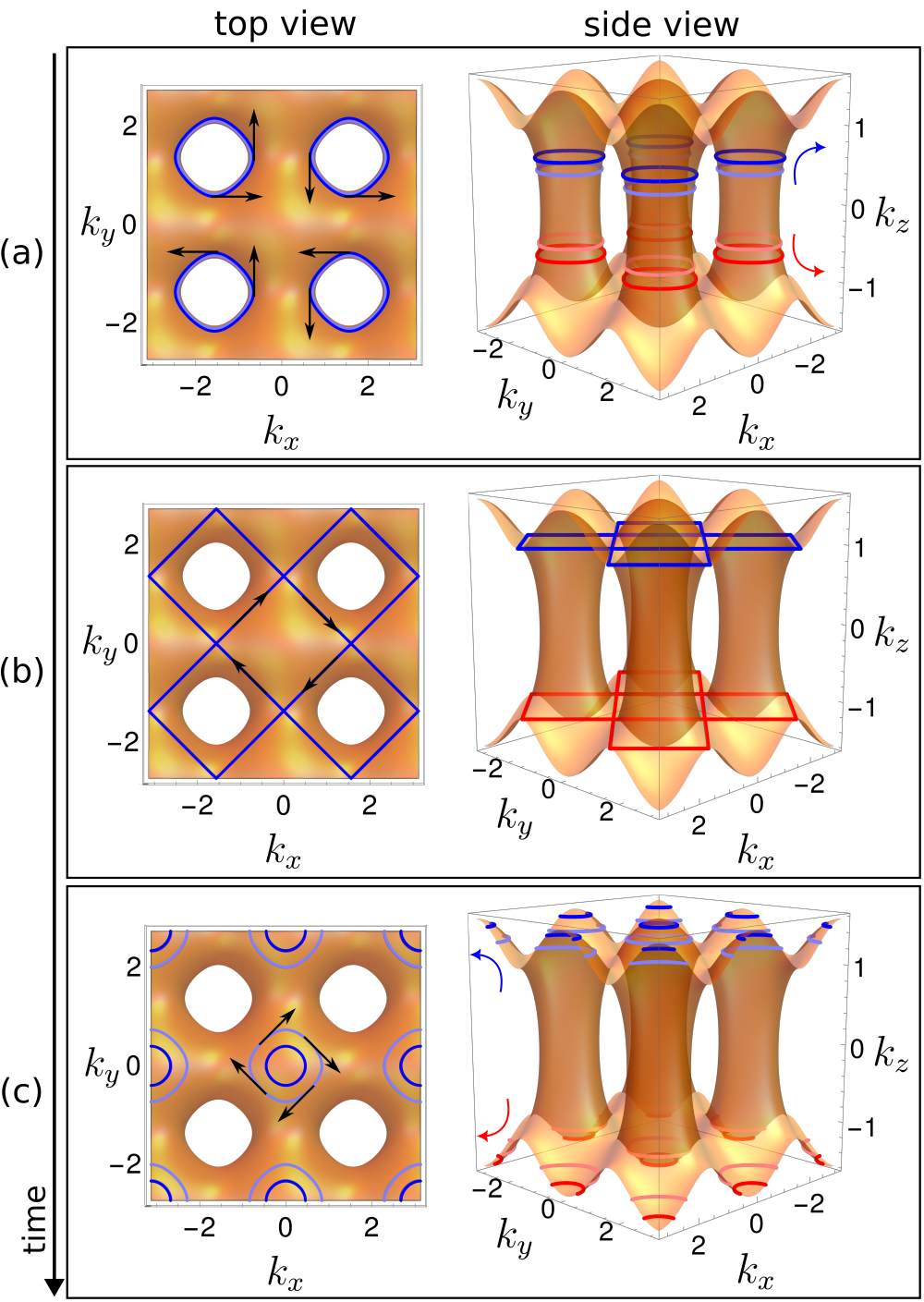
Figure 1: Exemplary dynamics of vortex loops on a static manifold $\mathcal{M}$ (orange surface) in a 3D BZ. The red and blue colors represent the chirality of the loops. (a) Incontractible loop with opposing chiralities are created in pairs and move in opposite directions; light colors correspond to $t=1.05$ and dark colors to $t=1.1$. (b) Loops of the same chirality can merge if their tangent vectors (black arrows) are antiparallel at the loops’ touching points. (c) Through loop merging, the loops can change their topological character from incontractible to contractible loops; $t=2$ (light colors), $t=3.5$ (dark colors).

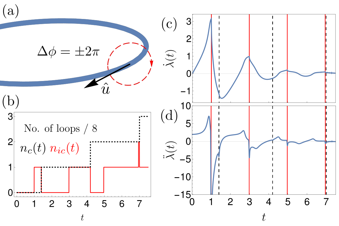
Figure 2: (a): Chirality ($\pm$) of a vortex loop is determined by $\Delta\phi=\pm 2\pi$ phase jump while encircling a loop around a tangent vector $\hat{u}$. (b): Number of contractable $n_{c}(t)$ and incontractible $n_{ic}(t)$ loops can be considered as quantized dynamical order parameters (black dashed and red solid lines, respectively). (c) and (d): The first and second derivative of the rate function $\lambda(t)$ with non-analytic DQPT points (marked by vertical lines), exactly match the changes of $n_{c}(t)$ and $n_{ic}(t)$.

The second condition in Eq. (7) defines a dynamical, equienergy surface that can intersect with $\mathcal{M}$ during some time intervals. The points at the intersection, where both conditions in Eq. (7) are satisfied simultaneously, represent the phase singularities of the Green’s function. While in a 2D case these singular points are isolated, in 3D they in general coalesce into 1D closed loops. These string-like structures are dynamic entities that exist on a static manifold $\mathcal{M}$. The vortex loops in different stages of evolution are illustrated in Fig. 1 by the blue and red curves.

As previously noted, the loops as closed curves on $\mathcal{M}$ can be categorized as either contractible or incontractible. In addition, the loops can also be characterized based on their chirality, indicated by $\pm$. Specifically, any closed curve circulating a vortex loop undergoes a phase jump of $\Delta\phi=\pm 2\pi$, where the sign of the jump represents the chirality of the loop. Loops’ chiralities are important in terms of their dynamics, e.g., loop merging or loop creation as explained in the following.

In a general scenario, the vortex loops are created at certain times, $t_{n}^{\mathrm{(}c)}=(2n\text{--}1)\pi/(2\epsilon_{\mathrm{max}})$, and annihilated at $t_{n}^{\mathrm{(}a)}=(2n\text{--}1)\pi/(2\epsilon_{\mathrm{min}})$, where $\epsilon_{\mathrm{max}}$ ($\epsilon_{\mathrm{min}}$) is the maximal (minimal) value of the upper band dispersion relation over quasi-momenta $\mathbf{k}$ belonging to $\mathcal{M}$, i.e., $\epsilon_{\mathrm{max}}=\max_{\mathbf{k}\in\mathcal{M}}\epsilon_{\mathbf{k}}$ ($\epsilon_{\mathrm{min}}=\max_{\mathbf{k}\in\mathcal{M}}\epsilon_{\mathbf{k}}$). As we show in Fig. 1 (a), the loops can be created (or annihiliated) in pairs with opposing chiralities, represented by red and blue colors. Alternatively, contractible loops can be also created from a single point of the BZ and annihilated in the inverse process. In the course of time evolution, the vortex loops of the same chirality can merge together as long as their tangent vectors at the touching point are antiparallel, for example, see Fig. 1 (b). Through the loop merging, it is even possible that the loops change their topological character, from incontractible to contractible [cf. Fig. 1 (c)], or vice versa.

The dynamics of vortex loops is rather complex, but can be captured qualitatively and quantitatively by monitoring the number of loops over time, denoted as $n_{c}(t)$ and $n_{ic}(t)$ for contractible and incontractible loops, respectively (Fig.2(b)). These numbers of vortices can be interpreted as quantized dynamical order parameters that distinguish between different non-equilibrium phases. To support this interpretation, we plot the first and second derivative of the rate function $\lambda(t)$, given by Eq.(5), in Fig.2 (b)-(c). In this work, we study a parameter quench from a normal insulator phase to a Weyl semimetal phase foo (c), which passes through a critical point of an equilibrium quantum phase transition, resulting in a change in the topological properties of the underlying Hamiltonian. Our analysis reveals a sequence of non-analytic points in time, which corresponds to a series of DQPT events, as per the definition Heyl (2018). Within our model, we observe two types of non-analytic points: those corresponding to a discontinuity in the second derivative of $\lambda(t)$ and those corresponding to a logarithmic divergence of $\ddot{\lambda}(t)$. By comparing the critical times with the number of vortex loops of each kind, we observe that the appearance of each non-analytic point is necessarily associated with a change in $n_{c}(t)$ or $n_{ic}(t)$.

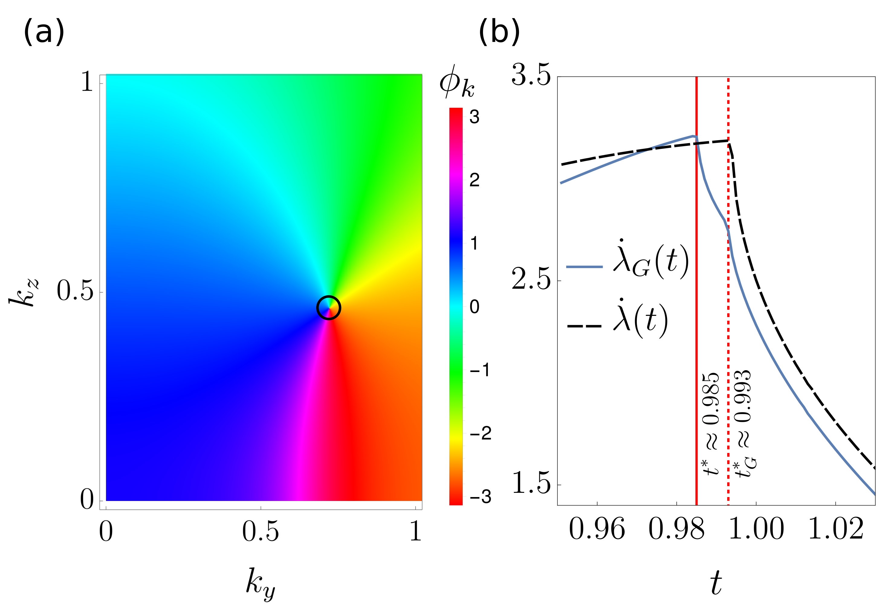
Figure 3: (a) The phase of the Green’s function $g_{\mathbf{k}}(t)$ in the interacting regime is shown for interaction strength $\eta=0.1$ and time $t=1.05$, with a fixed value of $k_{x}=\pi/2$. The black circle marks the position of the vortex in the non-interacting case. (b) The first derivative of the rate function $\lambda(t)$ (black dashed line) is plotted in the vicinity of the first non-analytic point in time, which occurs at $t^{*}\approx 0.985$ for $\eta=0.1$. The blue solid line represents the function $\lambda_{G}(t)$, cf. Eq. (10). The first temporal non-analytic point for $\lambda_{G}(t)$ occurs at a slightly later time, $t_{G}^{*}\approx 0.993$. Although the position of the vortex loops in momentum space is insensitive to perturbative interactions, the dynamics of the vortex loops and the dynamical quantum phase transition in the interacting case have no direct relationship, as discussed in the main text.

Effects of interactions. So far, we have focused on a non-interacting fermionic model. In this section we aim to demonstrate that our findings are more general and robust by showing that the vortex loops persist even in the presence of weak interactions. Consequently, let us consider $H=H_{0}+\eta V$, with $\eta$ being a small interaction strength and $V$ being a generic two-body interaction term To calculate the Green’s function $g_{\mathbf{k}}(t)$ in the interacting regime, the only difficulty lies in obtaining the time evolution operator in the interaction picture $U(t)$. However, up to linear order in $\eta$, we can utilize the Magnus expansion Magnus (1954); Blanes et al. (2009) and truncate $V$ to its leading terms Kriel et al. (2014) in order to approximate $U(t)\approx e^{-iH_{0}^{f}t}\exp\left(-\Omega\right)$ with

$$\Omega(t)\approx-i\eta t\sum_{\mathbf{k}}\sum_{\alpha,\beta}\Lambda_{\mathbf{k},\mathbf{k}^{\prime}}^{\alpha,\beta}\;\hat{n}_{\mathbf{k},\alpha}^{\textrm{(f)}}\hat{n}_{\mathbf{k^{\prime}},\beta}^{\textrm{(f)}},$$ (8)

where coefficients $\Lambda_{\mathbf{k},\mathbf{k}^{\prime}}^{\alpha,\beta}$ depend on the specific interaction type. Here, we choose BCS interactions and get $\Lambda_{\mathbf{k},\mathbf{k}^{\prime}}^{\alpha,\beta}=\delta_{\mathbf{k^{\prime}},\mathbf{\text{-}k}}|\gamma_{\mathbf{k},\uparrow}^{\alpha}|^{2}|\gamma_{\mathbf{k^{\prime}},\downarrow}^{\beta}|^{2}$ with $\gamma_{\mathbf{k},\sigma}^{\alpha}=$ $\langle\mathbf{k}_{\alpha}^{\textrm{(f)}}|\mathbf{k}_{\sigma}\rangle$, see foo (e). Inserting Eq. (8) into the formula for the Green’s function, Eq. (3), one readily gets

$$g_{\mathbf{k}}(t)\approx\sum_{\alpha,\beta}|\Gamma_{\mathbf{k},\alpha}\Gamma_{\text{-}\mathbf{k},\beta}|^{2}e^{it\epsilon_{\mathbf{k},\alpha}}e^{-it\left(\Lambda_{\mathbf{k},\text{-}\mathbf{k}}^{\alpha,\beta}+\Lambda_{\text{-}\mathbf{k},\mathbf{k}}^{\beta,\alpha}\right)}$$ (9)

with $\Gamma_{\mathbf{k}}^{\alpha}=\langle\mathbf{k}_{\alpha}^{(\mathrm{f})}|\mathbf{k}_{-}^{\mathrm{(i)}}\rangle$. Following these steps, in Fig. 3(a) we plot the phase of $g_{\mathbf{k}}(t)$, choosing the interaction strength $\eta=0.1$ and a time $t=1.05$. For clarity of the presentation we fix $k_{x}=\pi/2$ and illustrate a 2D cut through momentum space, which shows a clear phase singularity close to the center of the panel. Although the interacting part of the Hamiltonian adds a correction to the Green’s function, we find that within the numerical precision the position of the vortex in the momentum space matches the position of the vortex in the non-interacting case, marked by a black circle in Fig. 3(a). Consequently, we claim that the positions of the vortex loops are insensitive to perturbative interactions to leading order in the interaction strength.

As discussed previously, in the non-interacting system, the vortex loop dynamics is inherently imprinted in the rate function $\lambda(t)$. In the following we explore whether this relation still holds for the interacting case. In Fig. 3(b) we illustrate the first derivative of the rate function $\lambda(t)$ (the black dashed line) in the vicinity of the first non-analytic point in time, which, for $\eta=0.1$ is close to $t^{*}\approx 0.985$. In order to quantitatively determine the point in time associated with the loops’ creation and directly compare the behaviour of the Loschmidt amplitude and the Green’s function, we define

$$\lambda_{G}(t)=-\lim_{N\rightarrow\infty}\ln|\Pi_{\mathbf{k}}g_{\mathbf{k}}(t)|^{2}/N$$ (10)

and plot its first derivative in Fig. 3(b) (the blue solid line). We find that the first temporal non-analytic point appears for a slightly later time, $t_{G}^{*}\approx 0.993$. While this concludes that the dynamics of vortex loops and DQPTs in the interacting case are slightly shifted in time, it is noteworthy that it remains feasible to estimate the former by measuring the latter in experimental scenarios.

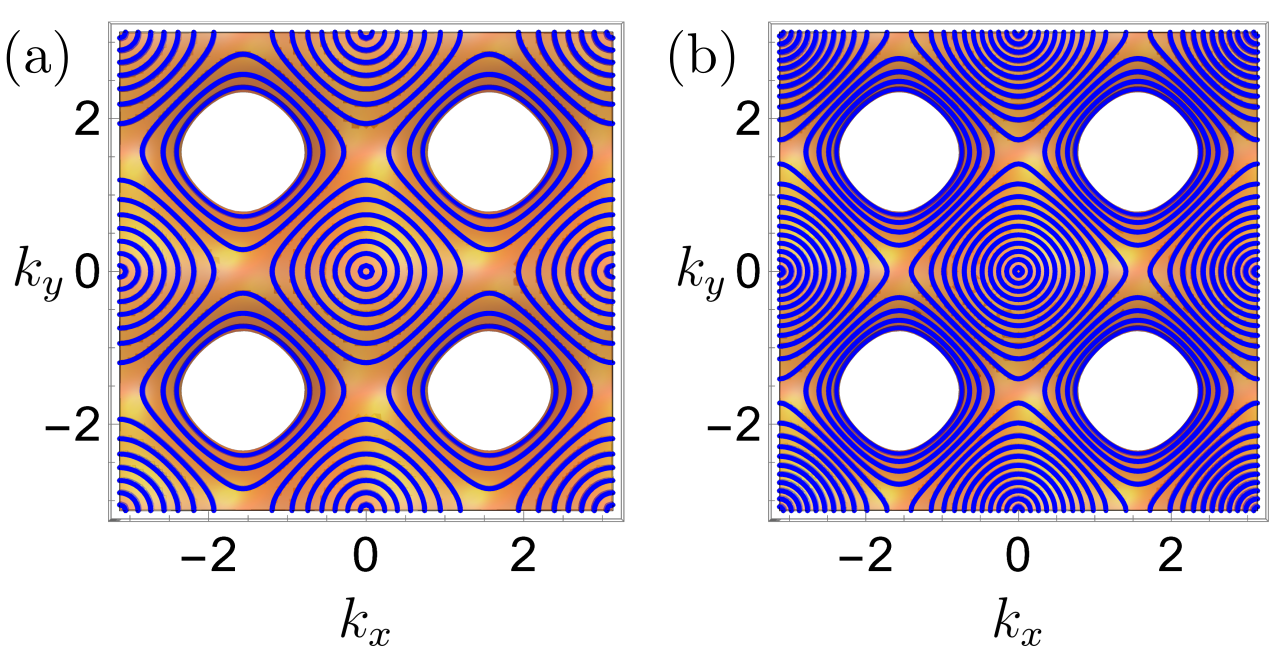
Figure 4: The complex pattern formed by loop vortices at times $t=15$ [panel (a)] and $t=30$ [panel (b)] after the quench to the Weyl semimetal phase, where the number of loops around the Weyl nodes increases linearly in time. Due to the dispersion relation $\epsilon_{\mathbf{k}}$ vanishing for some points belonging to the manifold $\mathcal{M}$, the loops never annihilate, and instead their dynamics slows down, leading to their accumulation around the band touching points $\mathbf{k}_{W}$. The resulting dynamical pattern cannot be destroyed due to the system’s dynamics.

Dynamical pattern formation. As mentioned earlier, we can obtain the creation and annihilation times of the loops from Eq.(7). The annihilation time is given by $t_{n}^{\mathrm{(a)}}=(2n-1)\pi/(2\epsilon_{\mathrm{min}})$, where $\epsilon_{\mathrm{min}}=\max_{\mathbf{k}\in\mathcal{M}}\epsilon_{\mathbf{k}}$. However, in our analysis presented in Fig.2(b), the total number of loops never decreases in time due to the choice of the model and the quench to the Weyl semimetal phase, which hosts pairs of the band touching Weyl nodes denoted by $\mathbf{k}_{W}$ foo (c). As the dispersion relation $\epsilon_{\mathbf{k}}$ vanishes for some points belonging to the manifold $\mathcal{M}$, the loops are never annihilated. Instead, the loops’ dynamics slow down, and eventually, they accumulate around the band touching points $\mathbf{k}_{W}$. In Fig. 4, we show a complex pattern formed by the loop vortices at times $t=15$ and $t=30$ after the quench. Although the number of loops around the Weyl nodes increases linearly in time, the resulting dynamical pattern cannot be destroyed due to dynamics.

Summary and perspectives. We have shown that after a parameter quench in three-dimensions the Green’s function of a general, fermionic model exhibits phase singularities in the form of dynamical 1D contractible or incontractible loops. We argue, that the number of these loops can be interpreted as two distinct, quantized order parameters that distinguish between different non-equilibrium phases, and show that changes in these order parameters are related to DQPTs. Moreover, we have shown that the vortex loops survive in weakly interacting systems, and that they can form complex dynamical patterns in momentum space due to the existence of band touching points.

Our findings reveal that non-equilibrium dynamics in 3D systems exhibit a significantly greater level of complexity compared to lower dimensions. As a result, it appears that to obtain a deeper understanding of the intricate out-of-equilibrium quantum phases of matter, there is a need to undertake further investigations on DQPTs specifically in 3D systems.

Acknowledgments. AK acknowledges the support of the Austrian Science Fund (FWF) within the ESPRIT Programme ESP 171-N under the Quantum Austria Funding Initiative. This project has received funding from the European Research Council (ERC) under the European Union’s Horizon 2020 research and innovation programme (grant agreement No. 853443).

Supplemental material

.1 Notation conventions for fermionic operators

In this section, for the convenience of a reader, we repeat the notation conventions for fermionic operators that we adopt throughout this article.

We consider spinful fermions on the lattice with the spin degrees of freedom denoted by $\sigma$. Unless stated otherwise, the spin takes to values: up ($\uparrow$) and down ($\downarrow$). The annihilation (creation) operators of fermions with a quasimomentum $\mathbf{k}$ and spin $\sigma$ read $\hat{c}_{\mathbf{k},\sigma}$ ($\hat{c}_{\mathbf{k},\sigma}^{\dagger}$). To study the time evolution it is convenient to work in a eigenbasis. For this reason we introduce annihilation operators of the initial and final Hamiltonian, $\hat{c}_{\mathbf{k},\alpha}^{\textrm{(i)}}$ and $\hat{c}_{\mathbf{k},\alpha}^{\textrm{(f)}}$, respectively, where the Greek letters $\alpha$ (or $\beta$) label energy bands. For the spin $1/2$ case, there are only two bands that we refer to as the lower ( - ) and higher ( + ) band. Since initially (i.e., before the quench) we are interested in the ground state of the system at half-filling,

$$|\psi_{0}\rangle=\Pi_{\mathbf{k}\in\mathrm{BZ}}|\mathbf{k}_{-}^{\mathrm{(i)}}\rangle,\quad|\mathbf{k}_{-}^{\mathrm{(i)}}\rangle=\hat{c}_{\mathbf{k},-}^{\mathrm{(}i)\dagger}|0\rangle\equiv\hat{c}_{\mathbf{k}}^{\mathrm{(}i)\dagger}|0\rangle$$ (S.1)

in this case, the band index always takes $\alpha=-$, and therefore throughout the main text we drop this subscript. (On the other hand, the energy band index cannot be dropped for the $\hat{c}_{\mathbf{k},\alpha}^{\textrm{(f)}}$ operators as the quench mixes the energy bands.)

The fermionic operators are related with linear transformations,

$$\hat{c}_{\mathbf{k},\sigma}^{\dagger}=\sum_{\alpha}\gamma_{\mathbf{k},\sigma}^{\alpha}\hat{c}_{\mathbf{k},\alpha}^{\textrm{(f)}\dagger}$$ (S.2)

with $\gamma_{\mathbf{k},\sigma}^{\alpha}=\langle\mathbf{k}_{\alpha}^{\mathrm{(f)}}|\mathbf{k}_{\sigma}\rangle$,

$$\hat{c}_{\mathbf{k},\sigma}^{\dagger}=\sum_{\alpha}\tilde{\gamma}_{\mathbf{k},\sigma}^{\alpha}\hat{c}_{\mathbf{k},\alpha}^{\textrm{(i)}\dagger}$$ (S.3)

with $\tilde{\gamma}_{\mathbf{k},\sigma}^{\alpha}=\langle\mathbf{k}_{\alpha}^{\mathrm{(i)}}|\mathbf{k}_{\sigma}\rangle$, and finally

$$\hat{c}_{\mathbf{k}}^{\textrm{(i)}\dagger}=\sum_{\alpha}\Gamma_{\mathbf{k}}^{\alpha}\hat{c}_{\mathbf{k},\alpha}^{\textrm{(f)}\dagger}$$ (S.4)

with $\Gamma_{\mathbf{k}}^{\alpha}=\langle\mathbf{k}_{\alpha}^{(\mathrm{f})}|\mathbf{k}_{-}^{\mathrm{(i)}}\rangle=\sum_{\sigma}\gamma_{\mathbf{k},\sigma}^{\alpha}\overline{\tilde{\gamma}_{\mathbf{k},\sigma}^{-}}$, where $\overline{[\cdot]}$ denotes the complex conjugation. The coefficients $\gamma_{\mathbf{k},\sigma}^{\alpha}$ and $\tilde{\gamma}_{\mathbf{k},\sigma}^{\alpha}$ can be easily calculated by explicitly diagonalizing $H_{\mathbf{k}}^{(\mathrm{i})}$ and $H_{\mathbf{k}}^{(\mathrm{f})}$, see Sec. .2.

.2 Eigenvectors of $H_{\mathbf{k}}$

For the completeness reasons here we give analytic expressions for eigenvalues and eigenvectors of $H_{\mathbf{k}}$. Any Hermitian $2\times 2$ matrix $H_{\mathbf{k}}$ can be decomposed in a matrix basis composed of the Pauli matrices $\vec{\sigma}=[\sigma_{x},\sigma_{y},\sigma_{z}]$ and the identity operator $\mathbb{1}$ as

$$H_{\mathbf{k}}=\vec{h}({\mathbf{k}})\cdot\vec{\sigma}+h_{0}({\mathbf{k}})\mathbb{1}$$ (S.5)

with $\vec{h}(\mathbf{k})=[h_{x}(\mathbf{k}),h_{y}(\mathbf{k}),h_{z}(\mathbf{k})]$ being a real valued vector. The eigenvectors of $H_{\mathbf{k}}$ can be simply expressed as

$$|\mathbf{k}_{+}\rangle = \sqrt{\frac{1+\hat{h}_{z}}{2}}|\mathbf{k}_{\uparrow}\rangle+\frac{\hat{h}_{x}+i\hat{h}_{y}}{\sqrt{2(1+\hat{h}_{z})}}\,|\mathbf{k}_{\downarrow}\rangle,$$ (S.6)

$$|\mathbf{k}_{-}\rangle = \frac{-\hat{h}_{x}+i\hat{h}_{y}}{\sqrt{2(1+\hat{h}_{z})}}\,|\mathbf{k}_{\uparrow}\rangle+\sqrt{\frac{1+\hat{h}_{z}}{2}}\,|\mathbf{k}_{\downarrow}\rangle,$$ (S.7)

where we denote $\hat{h}_{\alpha}=h_{\alpha}/|\vec{h}|$, $\alpha=x,y,z$. The corresponding eigenenergies read

$$\epsilon_{\pm}(\mathbf{k}) = h_{0}(\mathbf{k})\pm|\vec{h}(\mathbf{k})|$$ (S.8)

with $|\vec{h}|=\sqrt{h_{x}^{2}+h_{y}^{2}+h_{z}^{2}}$. Throughout the article we assume particle-hole symmetric systems which imply the condition $h_{0}(\mathbf{k})\equiv 0$ and $\epsilon_{\pm}(\mathbf{k})=\pm\epsilon(\mathbf{k})\equiv\pm|\vec{h}(\mathbf{k})|$. From the expression for the eigenstates one could readily read the coefficients of the transformation between the relevant fermionic operators, e.g.,

$$\gamma_{\mathbf{k},\uparrow}^{+}=\langle\mathbf{k}_{+}^{\mathrm{(f)}}|\mathbf{k}_{\uparrow}\rangle=\sqrt{[1+\hat{h}_{z}^{\textrm{(f)}}(\mathbf{k})]/2},\quad\mbox{etc.}$$ (S.9)

.3 Relation between the Green’s function and the first order correlation function

In the article we consider the time-ordered Green’s function

$$g_{\mathbf{k}}(t)=\sum_{\sigma}\langle\psi_{0}|\hat{c}_{\mathbf{k},\sigma}^{\dagger}(t)\hat{c}_{\mathbf{k},\sigma}|\psi_{0}\rangle,$$ (S.10)

where $|\psi_{0}\rangle$ is the fermionic ground state at half filling. By expanding the fermionic operators in the eigenbasis [cf. Sec. .1], we get

$$g_{\mathbf{k}}(t)=\sum_{\sigma}\sum_{\alpha,\beta}\overline{\tilde{\gamma}_{\mathbf{k},\sigma}^{\alpha}}\tilde{\gamma}_{\mathbf{k},\sigma}^{\beta}\langle\psi_{\mathbf{k},\text{-}\mathbf{k}}|\hat{c}^{\textrm{(i)}\dagger}_{\mathbf{k},\alpha}(t)\hat{c}^{\textrm{(i)}}_{\mathbf{k},\beta}|\psi_{\mathbf{k},\text{-}\mathbf{k}}\rangle$$ (S.11)

with $|\psi_{\mathbf{k},\text{-}\mathbf{k}}\rangle=|\mathbf{k}^{\textrm{(i)}}\rangle|\text{-}\mathbf{k}^{\textrm{(i)}}\rangle=\hat{c}_{\mathbf{k}}^{\textrm{(i)}\dagger}\hat{c}_{\text{-}\mathbf{k}}^{\textrm{(i)}\dagger}|0\rangle$ . Since

$$\hat{c}_{\mathbf{k},\beta}^{\textrm{(i)}}|\psi_{\mathbf{k},\text{-}\mathbf{k}}\rangle=\delta_{\beta,-}|\text{-}\mathbf{k}^{\textrm{(i)}}\rangle,$$ (S.12)

and using the fact that for a unitary transformation (S.3) we have

$$\sum_{\sigma}|\tilde{\gamma}_{\mathbf{k},\sigma}^{-}|^{2}=1,\quad\sum_{\sigma}\tilde{\gamma}_{\mathbf{k},\sigma}^{-}\tilde{\gamma}_{\mathbf{k},\sigma}^{+}=0,$$ (S.13)

we obtain

$$g_{\mathbf{k}}(t)=\langle 0|\hat{c}^{\mathrm{(i)}}_{\text{-}\mathbf{k}}\hat{c}^{\mathrm{(i)}}_{\mathbf{k}}\hat{c}_{\mathbf{k}}^{\mathrm{(i)}\dagger}(t)\hat{c}_{\text{-}\mathbf{k}}^{\mathrm{(i)}\dagger}|0\rangle.$$ (S.14)

In the non-interacting case (S.14) can be further simplified, namely

$$\begin{split}g_{\mathbf{k}}(t)=\langle 0|\hat{c}_{\mathbf{k}}^{\mathrm{(i)}}\hat{c}_{\mathbf{k}}^{\mathrm{(i)}\dagger}(t)|0\rangle\underbrace{\langle 0|\hat{c}_{\text{-}\mathbf{k}}^{\mathrm{(i)}}\hat{c}_{\text{-}\mathbf{k}}^{\mathrm{(i)}\dagger}|0\rangle}_{=1}=\langle 0|\hat{c}_{\mathbf{k}}^{\mathrm{(i)}}\hat{c}_{\mathbf{k}}^{\mathrm{(i)}\dagger}(t)|0\rangle\\ =\langle 0|\hat{c}_{\mathbf{k}}^{\mathrm{(i)}}U(t)^{\dagger}\hat{c}_{\mathbf{k}}^{\mathrm{(i)}\dagger}|0\rangle=\langle\mathbf{k}_{-}^{\mathrm{(i)}}(t)|\mathbf{k}_{-}^{\mathrm{(i)}}\rangle=\overline{\mathcal{G}_{\mathbf{k}}^{(1)}}(t).\end{split}$$ (S.15)

That is, in the non-interacting case, the Green’s function $g_{\mathbf{k}}(t)$ is a complex conjugate of the first order correlation function $\mathcal{G}_{\mathbf{k}}^{(1)}(t)$.

.4 Weyl semimetal

Weyl semimetals Weyl (1929); Delplace et al. (2012); Xu et al. (2015); Chen et al. (2015); Armitage et al. (2018); Wang et al. (2021) constitute a new topological gapless phase of matter that have recently gained significant attention in the field of condensed matter physics. Throughout the article we consider a special case of a simple two-band 3D Weyl semimetal Hamiltonian on the lattice Delplace et al. (2012); Chen et al. (2015), where

$$\vec{h}_{\mathbf{k}}=\left[\sin k_{x},\,\sin k_{y},\,m_{z}-\cos k_{z}\right]$$ (S.16)

with $m_{z}$ being a free parameter. As long as $|m_{z}|\leq 1$, the system is in the Weyl semimetal phase, whereas $|m_{z}|>1$ corresponds to a normal insulator. The Weyl semimetal phase hosts pairs of Weyl points (or nodes) located at distinct points in the BZ

$$\mathbf{k}_{W}=[n\pi,m\pi,\arccos(m_{z})]$$ (S.17)

with $m,n$ being integers, which are band touching points closing the energy gap. Diagonalizing the Hamiltonian $H_{\mathbf{k}}=\vec{h}_{\mathbf{k}}\cdot\vec{\sigma}$ gives the dispersion relation

$$\epsilon_{\mathbf{k},\pm}=\pm\sqrt{(\sin k_{x})^{2}+(\sin k_{y})^{2}+(m_{z}-\cos k_{z})^{2}}$$ (S.18)

which is linear around the $\mathbf{k}_{W}$ points, i.e.,

$$\epsilon_{\mathbf{k}_{W}+\hat{k}_{i}\delta k,\pm}\propto\pm\delta k$$ (S.19)

for $i=x,y,z$, featuring a gapless relativistic Dirac-like linear dispersion, analogous to the graphene but in three dimensions. One interesting aspect of Weyl semimetals on a lattice is that they show zero energy bulk states located at the nodes of opposite chirality, which are linked by topological surface Fermi arc excitations.Armitage et al. (2018). These unique electronic properties make them attractive candidates for various applications, including electronic and spintronic devices, as well as quantum computing.

While the properties of Weyl semimetals are indeed intriguing, their detailed description goes beyond the scope of this Letter. Our focus lies in the non-equilibrium dynamics of bulk states. Namely, we assume a parameter quench from a normal insulator phase to a Weyl semimetal phase, i.e., we choose $m_{z}=2.5$ and start with the ground state of the system, and at a time $t=0$ we change the parameter value to $m_{z}=0$. As the quench go through a critical point of an equilibrium quantum phase transition changing the topological properties of the underlying Hamiltonian, the quench is accompanied by a DQPT and consequently the appearance of 1D dynamical singularities in the phase of the Green’s function, which we describe in the main text of the article.

.5 Calculation of the evolution operator and correlation functions in the interacting case

We consider here interacting fermions $H=H_{0}+\eta V$, with $H_{0}$ being a non-interacting part, with $V$ being interaction term and $\eta$ being the interaction coupling strength. While in the analysis below $V$ can be an arbitrary momentum-conserving two-body interactions, for concreteness we choose

$$V=-\sum_{\mathbf{k},\mathbf{k}^{\prime}}\hat{c}_{\mathbf{k},\uparrow}^{\dagger}\hat{c}_{\mathbf{\text{-}k},\downarrow}^{\dagger}\hat{c}_{\mathbf{k}^{\prime},\uparrow}\hat{c}_{\mathbf{\text{-}k^{\prime}},\downarrow}$$ (S.20)

which describes BCS type interaction between the fermonic pairs of opposite momenta and spins. The full time evolution operator in the interaction picture can be written as

$$U(t)=U_{0}(t)W(t),\quad W(t)=\mathcal{T}e^{-i\eta\int_{0}^{t}dt^{\prime}V_{I}(t^{\prime})},$$ (S.21)

where $\mathcal{T}$ is the time ordering operator, $U_{0}(t)=e^{-iH_{0}^{f}t}$ is the time evolution operator of the non-interacting part of the quenched Hamiltonian and $V_{I}(t)=U_{0}(t)^{\dagger}VU_{0}(t)$. For a sufficiently small interaction coupling strength $\eta$, the interacting part can be written perturbatively Magnus (1954); Blanes et al. (2009) as

$$W(t)=e^{-\Omega(t)},$$ (S.22)

where $\Omega(t)$, the Magnus operator, in the first order of the perturbative expansion reads

$$\Omega(t)=i\eta\int_{0}^{t}dt^{\prime}V_{I}(t^{\prime}).$$ (S.23)

After expressing the fermionic operators in the post-quench non-interacting basis, we get

$$\Omega(t)=-i\eta\sum_{\mathbf{k},\mathbf{k}^{\prime}}\sum_{\alpha,\alpha^{\prime},\beta,\beta^{\prime}}V_{\mathbf{k},\mathbf{k}^{\prime}}^{\alpha,\alpha^{\prime},\beta,\beta^{\prime}}(t)\;\hat{c}_{\mathbf{k},\alpha}^{\textrm{(f)}\dagger}\hat{c}_{\mathbf{\text{-}k},\beta}^{\textrm{(f)}\dagger}\hat{c}_{\mathbf{\text{-}k^{\prime}},\beta^{\prime}}^{\textrm{(f)}}\hat{c}_{\mathbf{k}^{\prime},\alpha^{\prime}}^{\textrm{(f)}},$$ (S.24)

where

$$V_{\mathbf{k},\mathbf{k}^{\prime}}^{\alpha,\alpha^{\prime},\beta,\beta^{\prime}}(t)=\int\mbox{d}t\;\overline{\gamma_{\mathbf{k},\uparrow}^{\alpha}}(t)\gamma_{\mathbf{k}^{\prime},\uparrow}^{\alpha^{\prime}}(t)\overline{\gamma_{\text{-}\mathbf{k},\downarrow}^{\beta}}(t)\gamma_{\text{-}\mathbf{k}^{\prime},\downarrow}^{\beta^{\prime}}(t)$$ (S.25)

and $\gamma_{\mathbf{k},\sigma}^{\alpha}(t)=\langle\mathbf{k}_{\alpha}^{\textrm{(f)}}|\mathbf{k}_{\sigma}\rangle e^{-i\epsilon_{\mathbf{k},\alpha}t},$ see Sec. .1.

The Magnus operator can be further simplified if we neglect the off-diagonal terms Kriel et al. (2014), i.e., in the following we approximate

$$\Omega(t)\approx-i\eta t\sum_{\mathbf{k}}\sum_{\alpha,\beta}\Lambda_{\mathbf{k},\text{-}\mathbf{k}}^{\alpha,\beta}\;\hat{n}_{\mathbf{k},\alpha}^{\mathrm{(f)}}\hat{n}_{\mathbf{\text{-}k},\beta}^{\mathrm{(f)}},$$ (S.26)

with

$$\Lambda_{\mathbf{k},\text{-}\mathbf{k}}^{\alpha,\beta}=\big{|}\gamma_{\mathbf{k},\uparrow}^{\alpha}\big{|}^{2}\big{|}\gamma_{\mathbf{\text{-}k},\downarrow}^{\beta}\big{|}^{2}.$$ (S.27)

Now, we can easily calculate the time dependent fermionic operators, namely,

$$\hat{c}_{\mathbf{k},\alpha}^{\mathrm{(f)}}(t)=U^{\dagger}\hat{c}_{\mathbf{k},\alpha}^{\mathrm{(f)}}U=\tilde{U}_{\mathbf{k},\alpha}^{\dagger}(t)\hat{c}_{\mathbf{k},\alpha}^{\mathrm{(f)}},$$ (S.28)

where

$$\tilde{U}_{\mathbf{k},\alpha}(t)=e^{-it\epsilon_{\mathbf{k},\alpha}}e^{it\sum_{\beta}\left(\Lambda_{\mathbf{k},\text{-}\mathbf{k}}^{\alpha,\beta}+\Lambda_{\text{-}\mathbf{k},\mathbf{k}}^{\beta,\alpha}\right)\hat{n}_{\text{-}\mathbf{k},\beta}^{\mathrm{(f)}}}.$$ (S.29)

Subsequently, using the formula (S.14) for the Green’s function, it is now straightforward to calculate the Green’s function

$$g_{\mathbf{k}}(t)=\sum_{\alpha,\beta}|\Gamma_{\mathbf{k}}^{\alpha}\Gamma_{\text{-}\mathbf{k}}^{\beta}|^{2}e^{it\epsilon_{\mathbf{k},\alpha}}e^{-it\left(\Lambda_{\mathbf{k},\text{-}\mathbf{k}}^{\alpha,\beta}+\Lambda_{\text{-}\mathbf{k},\mathbf{k}}^{\beta,\alpha}\right)}.$$ (S.30)

Analogously, we can readily obtain the Loschmidt amplitude in the interacting case,

$$\mathcal{G}(t)=\Pi_{\mathbf{k}|k_{x}>0}\sum_{\alpha,\beta}|\Gamma_{\mathbf{k}}^{\alpha}\Gamma_{\text{-}\mathbf{k}}^{\beta}|^{2}e^{it\left(\epsilon_{\mathbf{k},\alpha}+\epsilon_{\text{-}\mathbf{k},\beta}-\Lambda_{\mathbf{k},\text{-}\mathbf{k}}^{\alpha,\beta}-\Lambda_{\text{-}\mathbf{k},\mathbf{k}}^{\beta,\alpha}\right)}.$$ (S.31)

References

- Polkovnikov et al. (2011) A. Polkovnikov, K. Sengupta, A. Silva, and M. Vengalattore, Reviews of Modern Physics 83, 863 (2011), URL https://doi.org/10.1103/revmodphys.83.863.
- Mori et al. (2018) T. Mori, T. N. Ikeda, E. Kaminishi, and M. Ueda, Journal of Physics B: Atomic, Molecular and Optical Physics 51, 112001 (2018), URL https://doi.org/10.1088/1361-6455/aabcdf.
- Moudgalya et al. (2022) S. Moudgalya, B. A. Bernevig, and N. Regnault, Reports on Progress in Physics 85, 086501 (2022), URL https://doi.org/10.1088/1361-6633/ac73a0.
- Abanin et al. (2019) D. A. Abanin, E. Altman, I. Bloch, and M. Serbyn, Reviews of Modern Physics 91 (2019), URL https://doi.org/10.1103/revmodphys.91.021001.
- Khemani et al. (2019) V. Khemani, R. Moessner, and S. L. Sondhi, A brief history of time crystals (2019), eprint 1910.10745.
- Sacha (2020) K. Sacha, Time Crystals (Springer International Publishing, 2020), URL https://doi.org/10.1007/978-3-030-52523-1.
- Sachdev (2000) S. Sachdev, Quantum Phase Transitions (Cambridge University Press, 2000), URL https://doi.org/10.1017/cbo9780511622540.
- Dziarmaga (2010) J. Dziarmaga, Advances in Physics 59, 1063 (2010), URL https://doi.org/10.1080/00018732.2010.514702.
- Heyl et al. (2013) M. Heyl, A. Polkovnikov, and S. Kehrein, Physical Review Letters 110 (2013), URL https://doi.org/10.1103/physrevlett.110.135704.
- Zvyagin (2016) A. A. Zvyagin, Low Temperature Physics 42, 971 (2016), URL https://doi.org/10.1063/1.4969869.
- Heyl (2018) M. Heyl, Reports on Progress in Physics 81, 054001 (2018), URL https://doi.org/10.1088/1361-6633/aaaf9a.
- Heyl (2019) M. Heyl, EPL (Europhysics Letters) 125, 26001 (2019), URL https://doi.org/10.1209/0295-5075/125/26001.
- Budich and Heyl (2016) J. C. Budich and M. Heyl, Phys. Rev. B 93, 085416 (2016), URL https://link.aps.org/doi/10.1103/PhysRevB.93.085416.
- Halimeh and Zauner-Stauber (2017) J. C. Halimeh and V. Zauner-Stauber, Phys. Rev. B 96, 134427 (2017), URL https://link.aps.org/doi/10.1103/PhysRevB.96.134427.
- Žunkovič et al. (2018) B. Žunkovič, M. Heyl, M. Knap, and A. Silva, Phys. Rev. Lett. 120, 130601 (2018), URL https://link.aps.org/doi/10.1103/PhysRevLett.120.130601.
- Lang et al. (2018) J. Lang, B. Frank, and J. C. Halimeh, Phys. Rev. Lett. 121, 130603 (2018), URL https://link.aps.org/doi/10.1103/PhysRevLett.121.130603.
- Heyl et al. (2018) M. Heyl, F. Pollmann, and B. Dóra, Phys. Rev. Lett. 121, 016801 (2018), URL https://link.aps.org/doi/10.1103/PhysRevLett.121.016801.
- Kosior and Sacha (2018) A. Kosior and K. Sacha, Physical Review A 97 (2018), URL https://doi.org/10.1103/physreva.97.053621.
- Kosior et al. (2018) A. Kosior, A. Syrwid, and K. Sacha, Physical Review A 98 (2018), URL https://doi.org/10.1103/physreva.98.023612.
- Yang et al. (2019) K. Yang, L. Zhou, W. Ma, X. Kong, P. Wang, X. Qin, X. Rong, Y. Wang, F. Shi, J. Gong, et al., Phys. Rev. B 100, 085308 (2019), URL https://link.aps.org/doi/10.1103/PhysRevB.100.085308.
- Zhou and Du (2021) L. Zhou and Q. Du, New Journal of Physics 23, 063041 (2021), URL https://doi.org/10.1088/1367-2630/ac0574.
- Peotta et al. (2021) S. Peotta, F. Brange, A. Deger, T. Ojanen, and C. Flindt, Phys. Rev. X 11, 041018 (2021), URL https://link.aps.org/doi/10.1103/PhysRevX.11.041018.
- Trapin et al. (2021) D. Trapin, J. C. Halimeh, and M. Heyl, Phys. Rev. B 104, 115159 (2021), URL https://link.aps.org/doi/10.1103/PhysRevB.104.115159.
- Bandyopadhyay et al. (2021) S. Bandyopadhyay, A. Polkovnikov, and A. Dutta, Physical Review Letters 126 (2021), URL https://doi.org/10.1103/physrevlett.126.200602.
- Halimeh et al. (2021) J. C. Halimeh, D. Trapin, M. Van Damme, and M. Heyl, Phys. Rev. B 104, 075130 (2021), URL https://link.aps.org/doi/10.1103/PhysRevB.104.075130.
- De Nicola et al. (2021) S. De Nicola, A. A. Michailidis, and M. Serbyn, Phys. Rev. Lett. 126, 040602 (2021), URL https://link.aps.org/doi/10.1103/PhysRevLett.126.040602.
- Fläschner et al. (2017) N. Fläschner, D. Vogel, M. Tarnowski, B. S. Rem, D.-S. Lühmann, M. Heyl, J. C. Budich, L. Mathey, K. Sengstock, and C. Weitenberg, Nature Physics 14, 265 (2017), URL https://doi.org/10.1038/s41567-017-0013-8.
- Zhang et al. (2017) J. Zhang, G. Pagano, P. W. Hess, A. Kyprianidis, P. Becker, H. Kaplan, A. V. Gorshkov, Z.-X. Gong, and C. Monroe, Nature 551, 601 (2017), URL https://doi.org/10.1038/nature24654.
- Guo et al. (2019) X.-Y. Guo, C. Yang, Y. Zeng, Y. Peng, H.-K. Li, H. Deng, Y.-R. Jin, S. Chen, D. Zheng, and H. Fan, Phys. Rev. Appl. 11, 044080 (2019), URL https://link.aps.org/doi/10.1103/PhysRevApplied.11.044080.
- Tian et al. (2020) T. Tian, H.-X. Yang, L.-Y. Qiu, H.-Y. Liang, Y.-B. Yang, Y. Xu, and L.-M. Duan, Phys. Rev. Lett. 124, 043001 (2020), URL https://link.aps.org/doi/10.1103/PhysRevLett.124.043001.
- Jurcevic et al. (2017) P. Jurcevic, H. Shen, P. Hauke, C. Maier, T. Brydges, C. Hempel, B. P. Lanyon, M. Heyl, R. Blatt, and C. F. Roos, Phys. Rev. Lett. 119, 080501 (2017), URL https://link.aps.org/doi/10.1103/PhysRevLett.119.080501.
- Yuzbashyan et al. (2006) E. A. Yuzbashyan, O. Tsyplyatyev, and B. L. Altshuler, Physical Review Letters 96 (2006), URL https://doi.org/10.1103/physrevlett.96.179905.
- Sciolla and Biroli (2010) B. Sciolla and G. Biroli, Physical Review Letters 105 (2010), URL https://doi.org/10.1103/physrevlett.105.220401.
- Halimeh et al. (2017) J. C. Halimeh, V. Zauner-Stauber, I. P. McCulloch, I. de Vega, U. Schollwöck, and M. Kastner, Phys. Rev. B 95, 024302 (2017), URL https://link.aps.org/doi/10.1103/PhysRevB.95.024302.
- Marino et al. (2022) J. Marino, M. Eckstein, M. S. Foster, and A. M. Rey, Reports on Progress in Physics 85, 116001 (2022), URL https://doi.org/10.1088/1361-6633/ac906c.
- Vajna and Dóra (2014) S. Vajna and B. Dóra, Phys. Rev. B 89, 161105 (2014), URL https://link.aps.org/doi/10.1103/PhysRevB.89.161105.
- Yu (2017) J. Yu, Phys. Rev. A 96, 023601 (2017), URL https://link.aps.org/doi/10.1103/PhysRevA.96.023601.
- Qiu et al. (2018) X. Qiu, T.-S. Deng, G.-C. Guo, and W. Yi, Phys. Rev. A 98, 021601 (2018), URL https://link.aps.org/doi/10.1103/PhysRevA.98.021601.
- Lahiri and Bera (2019) A. Lahiri and S. Bera, Phys. Rev. B 99, 174311 (2019), URL https://link.aps.org/doi/10.1103/PhysRevB.99.174311.
- Sim et al. (2022) K. Sim, R. Chitra, and P. Molignini, Phys. Rev. B 106, 224302 (2022), URL https://link.aps.org/doi/10.1103/PhysRevB.106.224302.
- Tarnowski et al. (2019) M. Tarnowski, F. N. Ünal, N. Fläschner, B. S. Rem, A. Eckardt, K. Sengstock, and C. Weitenberg, Nature Communications 10 (2019), URL https://doi.org/10.1038/s41467-019-09668-y.
- Weyl (1929) H. Weyl, Zeitschrift für Physik 56, 330 (1929), URL https://doi.org/10.1007/bf01339504.
- Delplace et al. (2012) P. Delplace, J. Li, and D. Carpentier, EPL (Europhysics Letters) 97, 67004 (2012), URL https://doi.org/10.1209/0295-5075/97/67004.
- Xu et al. (2015) S.-Y. Xu, I. Belopolski, N. Alidoust, M. Neupane, G. Bian, C. Zhang, R. Sankar, G. Chang, Z. Yuan, C.-C. Lee, et al., Science 349, 613 (2015), URL https://doi.org/10.1126/science.aaa9297.
- Chen et al. (2015) C.-Z. Chen, J. Song, H. Jiang, Q. feng Sun, Z. Wang, and X. Xie, Physical Review Letters 115 (2015), URL https://doi.org/10.1103/physrevlett.115.246603.
- Armitage et al. (2018) N. Armitage, E. Mele, and A. Vishwanath, Reviews of Modern Physics 90 (2018), URL https://doi.org/10.1103/revmodphys.90.015001.
- Wang et al. (2021) Z.-Y. Wang, X.-C. Cheng, B.-Z. Wang, J.-Y. Zhang, Y.-H. Lu, C.-R. Yi, S. Niu, Y. Deng, X.-J. Liu, S. Chen, et al., Science 372, 271 (2021), URL https://doi.org/10.1126/science.abc0105.
- foo (a) See the Supplemental Material for a brief summary on notation convention for fermionic operators used in this manuscript.
- foo (b) See the Supplemental Material for a discussion on eigenstates of .
- Peskin (2018) M. E. Peskin, An Introduction To Quantum Field Theory (CRC Press, 2018), URL https://doi.org/10.1201/9780429503559.
- foo (c) See the Supplemental Material for a more detailed discussion on Weyl Hamitlonian, its eigenergies and Weyl nodes.
- foo (d) See the Supplemental Material for a calculation demonstrating the connection between the Green’s function and the first-order correlation function.
- Zache et al. (2019) T. V. Zache, N. Mueller, J. T. Schneider, F. Jendrzejewski, J. Berges, and P. Hauke, Phys. Rev. Lett. 122, 050403 (2019), URL https://link.aps.org/doi/10.1103/PhysRevLett.122.050403.
- Hirzebruch (1966) F. Hirzebruch, Topological Methods in Algebraic Geometry (Springer Berlin Heidelberg, 1966), URL https://doi.org/10.1007/978-3-642-62018-8.
- Magnus (1954) W. Magnus, Communications on Pure and Applied Mathematics 7, 649 (1954), URL https://doi.org/10.1002/cpa.3160070404.
- Blanes et al. (2009) S. Blanes, F. Casas, J. Oteo, and J. Ros, Physics Reports 470, 151 (2009), URL https://doi.org/10.1016/j.physrep.2008.11.001.
- Kriel et al. (2014) J. N. Kriel, C. Karrasch, and S. Kehrein, Phys. Rev. B 90, 125106 (2014), URL https://link.aps.org/doi/10.1103/PhysRevB.90.125106.
- foo (e) See the Supplemental Material for a calculation of the evolution operator and correlation functions in the interacting case.