Intracellular Dynamics of Hepatitis B Virus Infection: A Mathematical Model and Global Sensitivity Analysis of Its Parameters

1 Abstract

Analysis of cell population can reveal the average information about the viral infection in host whereas single-cell analysis can capture the individual consideration. Single-cell analysis can also provide new ways to explore viral diversities and identify the intrinsic extreme phenotype of the cells. In this study, a single-cell hepatitis B virus (HBV) infection model is proposed by considering all possible intracellular steps which are observed in the viral life cycle. To the best of our knowledge, it is the most generalized model to date. The effects of newly introduced factors or components such as, cccDNA, HBx proteins, surface proteins, and double-stranded linear DNA-containing capsids are explained very well by this model. The intracellular delay is also incorporated into the proposed model, and it is seen that it has no significant impacts on the persistence of infection. The global sensitivity analysis of the parameters is also performed using partial rank correlation coefficients based on Latin hypercube sampling method. According to PRCC values, the most positive and most negative sensitive parameters are identified. Moreover, it is observed that availability of viral surface proteins switches the replication pattern from acute to chronic, whereas there is no considerable contribution of HBx proteins to the progression of HBV infection. Another striking result is that the recycling of capsids appears to act as a positive feedback loop throughout the infection.
Keywords: Single-cell model, Hepatitis B, cccDNA, Global sensitivity analysis, Partial rank correlation coefficient

2 Introduction

Hepatitis B virus (HBV) belongs to the family of Hepadnaviridae. It is a non-cytopathic virus that causes various kinds of serious liver disease such as liver damage, cirrhosis, liver cancer or hepatocellular carcinoma (HCC). HCC is the second leading cause of cancer-related death in human. Currently, HBV is one of the most common liver infections and a global public health problem worldwide. It has the potential to spread 100 times more than HIV/AIDS [1]. HBV has affected two billion individuals throughout the world. Every year at around 1.5 million people become newly infected despite the existence of effective vaccine. Almost 300 million people are chronically infected. At around 10% of infected persons are diagnosed, and an estimated 820,000 people die each year as a result of HBV infection and accompanying consequences, such as liver cancer [2].

There are many limitations to the current treatment procedures, which often fail to provide long-term virologic control. The majority of the infected people require lifelong therapy if it is once initiated because the current treatments can only reduce the possible risks of progressing cirrhosis and hepatocellular carcinoma [1]. Most of the time, the available treatments can usually cure the disease. It is true that there are some approved antiviral drugs, including interferons (IFN)-alpha-2a, pegylated (PEG)-IFN-alpha-2a (immune system modulators), and some nucleoside analogues, such as lamivudine, adefovir, entecavir, telbivudine, and tenofovir. But no single therapy is sufficient to diagnose a chronic HBV patient [3]. As a result of discontinuation of antiviral therapy, unfortunately viruses often rebound [4]. A lot of evidences prove that the persistence of covalently closed circular DNA (cccDNA) is one of the major obstacle to prevent this viral infection[5]. There are some other reasons for this, including the fact that HBV is a DNA virus and its replication process is very complicated compared to that of other viruses, deficiency of immune responses, drug-drug intersection and drug resistance [6], etc. Although a lot of studies have been done over the last two decades, the dynamics of this viral infection is not yet well understood.

Most of previous studies [7, 8, 9] of this viral infection have mainly concentrated on the cell population. By analyzing the cell population, one can get a general overview of the clinical signs and progression of viral infection. In order to investigate the cell activities throughout the infection period and response of immune system against virus, cell population analysis is an important and useful tool. In a cell population, there are several types of cells that can differ in identity, state, functions, etc. Naturally, cells are heterogeneous, and it occurs in cells because of variation in DNA sequence [10]. In the literature, it is seen that when cell populations are considered to study any kind of viral infection, the total number of cells are divided into two classes: uninfected and infected cells. Due to this classification, some salient features of the cells, the roles of some specific phenotypes, the impacts of some intracellular components of virus and the effects of several parameters involved in the infection have been overlooked [11, 12]. Thus, it is important to explore intrinsic processes at the level of single cells. In 1940, Delbruck considered the phage-infected E.coli cells to study the heterogeneity of virus infected cell. In this experiment, it is observed that the amount of progeny virus released from each cell differs significantly which revealed a surprisingly broad distribution of virus growth throughout the infection [13]. With the development of single-cell technologies, infection kinetics and quantification of burst size of vesicular stomatitis virus (VSV) have been studied. The virus titers differ from cell to cell during viral infection which suggest a high degree of cell to cell variation [14, 15]. According to some recent studies on influenza A virus (IAV), foot-and-mouth-disease (FMD) virus (FMDV), and poliovirus, virion levels varied from cell to cell unlike phenomena observed in experiments involving multicellular populations [16, 17, 18]. Zhu et al. [19] found that the cell size and cell cycle of the host are also two major factors that contribute to the variability of virus yields among single cells.

Nowadays, single-cell analyses become a significant milestone in many fields, including immunology, oncology, stem cells, virology, etc [20, 21, 22, 23]. The following are some key advantages of single-cell analysis in virology:

1. The dynamics of infection in each infected cell can be studied at the micro level.

2. The intracellular components of the virus that have significant influence on infection can be identified.

3. One can determine the most sensitive parameter for an infection.

4. A large cell population analysis may overlook individual cell responses to the viruses under viral infection period.

5. Because of the inherent heterogeneity in healthy and diseased cells, drug discovery & development, diagnostics, and prognostics encounter significant obstacles. These challenges can be mitigated by analyzing infected single cells.

Viral infections involve multiple steps that include attachment & entry, genome trafficking, fusion, nuclear import, expressing viral genes, replication of the genome, and releasing progeny. In case of HBV, there are some additional steps in the replication process, such as rcDNA repairing, translation, transcription, reverse transcription, recycling of capsids, which complicates the viral life cycle [24, 25]. This infection can be spread in two ways: cell-to-cell and virus-to-cell. The primary mode of infection transmission during hepatitis B virus infection is cell-to-cell transmission [26]. Although many authors have attempted to study this virus infection from different perspectives, the goal of curing this disease remains a challenging task. For example, in 1996, Nowak et al. [27] presented basic model of virus dynamics considering three compartments: uninfected cells, infected cells and viruses. Min et al. [8] modified this basic model [27] by replacing the mass action term with standard incidence function (SIF) and concluded that SIF is more appropriate than mass action term to describe this kind of viral infection kinetics. Liu et al. [9] studied a modified age-structure model and proved that the age of infected hepatocytes plays a crucial role in HBV infection. The host immune response holds significant role in regulating this viral infection. [28]. Two main factors in immune-mediated clearance are CTL and non-CTL effects, although the CTL effects cannot eliminate the infection on its own [29]. Fatehi et al. [30] found that natural killer cell which is a part of innate immune system, kills the infected hepatocytes by producing perforin and granzymes. On the other hand, rather than rapid release of HBV virion from infected hepatocytes, the accumulation of HBV DNA-containing capsid in the infected cell increases the risk of exacerbation of hepatitis [31].

Besides the studies mentioned above, a variety of mathematical models [7, 32, 33] have been developed to investigate the dynamics of HBV transmission. Most of them considered the large cell population. In this study, an intracellular dynamics model is proposed based on the biological and clinical findings with some basic assumptions. All possible intracellular components of virus life cycle (rcDNA, cccDNA, HBx-proteins, polymerase, surface proteins, single stranded and double-stranded DNA, double-stranded linear DNA, etc) and parameters associated with the infection are considered in this model in order to make it more realistic and reliable. To the best of our knowledge, it is the first intracellular model that depicts all possible targets by various antiviral techniques. The following topics are discussed in this study as main contributions:

1. The effects of initial concentration of cccDNAs in HBV infection dynamics.

2. Effects of HBx proteins on infection.

3. The roles of intracellular delay in disease dynamics.

4. Impacts of surface proteins on infection.

5. The contributions of double-stranded linear DNA-containing capsids on cccDNA as well as on virus.

6. Recycling mechanism of double-stranded DNA-containing capsids.

7. The global sensitivity analysis of model parameters.

3 Model Formulation

Figure 1: Schematic representation of the HBV replication process in liver cells. The numerical sequence of steps is not indicative of the underlying biological processes, but rather serves as a tool to aid our understanding.

3.1 Intracellular dynamics model

HBV is a member of the hepadnaviridae family and by virtue of its exceptional characteristics, it replicates through RNA intermediates similarly as retroviruses. In this way, the replication cycle of HBV is able to perpetuate the infection in hepatocytes through its unique features [34]. HBV replication begins when the virus enters the liver cells through the sodium taurocholate cotransporting polypeptide (NTCP) receptor via receptor-mediated endocytosis. Although, at first, HBV binds to heparan sulfate proteoglycans (HSPGs) with a low affinity. Inside the hepatocytes, virus releases its core particle i.e. relaxed circular DNA (rcDNA) containing capsids (Step 1: Figure 1). This model does not explicitly include the role of NTCP and HSPGs receptors in HBV entry. Our study focuses on intracellular infection dynamics of HBV. The number of viruses and rcDNA-containing capsids are designated by $V$ and $R$, respectively. It is considered that the viruses uncoat their core particle with the rate $\alpha_{1}$ and $\delta_{r}$ is the decay rate of rcDNA. The parameter $\alpha_{2}$ represents the rate at which the cccDNA is formed from rcDNA , and it is discussed in detail below. The corresponding differential equation is:

$$\frac{dR}{dt}=\alpha_{1}V-\alpha_{2}R-\delta_{r}R.$$ (1)

In order to release the viral genome (rcDNA), HBV nucleocapsids travel to the nucleus of hepatocytes. In order to overcome the high viscosity of the cytoplasm, HBV utilizes the microtubular network for efficient nuclear delivery. In addition, microtubule-dependent movement may also provide direct path to the nucleus periphery. In the cytoplasm (or at the nuclear pore), capsids are disassembled or partially disassembled. This causes the signal for nuclear localization (NLS) to be exposed. After the interaction of NLS with the capsids, the capsids attach to nuclear transport factors (importin $\alpha$ and $\beta$) and are transported into the nuclear baskets. The nuclear pores complex (NPC), which serves as a gatekeeper to the nucleus, plays an important role in the entry of HBV genomes into the nucleus. Mature capsids bind to nucleoporin 153 (Nup 153) in the nuclear basket, enter the nucleus, and disintegrate to release the viral genome. In the first step after genome entry, the rcDNA is repaired by the host DNA repair mechanism and is converted to covalently closed circular DNA (cccDNA) (Step 2: Figure 1). We denote the cccDNAs by $C$. There are different ways in which cccDNAs are lost, such as cell proliferation, cell death due to cytolytic immune response, cell cure due to non-cytolytic immune response, and natural death of infected cell. Only the natural decay rate of cccDNAs $(\delta_{c})$ is considered in this model. This reaction is described as

$$\frac{dC}{dt}=\alpha_{2}R+k_{1}e^{-\lambda S_{p}}D-\delta_{c}C.$$ (2)

Here, the term $k_{1}e^{-\lambda S_{p}}D$ represents the recycling of rcDNA-containing capsids. The details about the recycling of capsids are discussed later. In HBV replication, cccDNA plays a key role in transcription. In the nucleus, cccDNA forms minichromosomes that are the source of pregenomic RNA (pgRNA) and other viral RNAs. There are five different sets of mRNAs generated from the viral cccDNA and are encoded by the four main genes through a series of long overlapping reading frames [35]. The mRNAs are: three subgenomic mRNA (0.7 kb mRNA, 2.1 kb mRNA and 2.4 kb mRNA ) and two gemomics mRNA of 3.5 kb. These are all heterogeneous and positively oriented [36]. 3.5 kb mRNA is designated by $R_{g}$. As both 2.4 kb mRNA and 2.1 kb mRNA produce surface proteins, these are treated as a single compartment by $R_{s}$ in our model. 0.7 kb mRNA is represented by $R_{h}$. The parameters $\lambda_{rg},\lambda_{rs}\leavevmode\nobreak\ \mbox{and}\leavevmode\nobreak\ \lambda_{rh}$ are the transcription rates of 3.5 kb mRNA, (2.4 kb mRNA and 2.1 kb mRNA) and 0.7 kb mRNA, respectively. HBV X protein (HBx), which is produced from 0.7 kb mRNA, denoted by $H$, prevents cccDNA from becoming silent. Only HBx acts as a sole regulator protein. It possesses multi-functional roles. HBx promotes the degradation of structural maintenance of chromosome and can enhance the transcription rate of cccDNA [37]. In addition, HBx inhibits the development of immune response to HBV infection, preventing apoptosis of infected hepatocytes [38, 39]. Therefore, HBx plays some important roles in HBV replication. In this study, the functions of HBx are included. Mathematically, these are described as follows (Step 3a, 3b, 3c: Figure 1):

$$\frac{dR_{g}}{dt}=\lambda_{rg}\Phi C-\mu_{1}R_{g}P-\delta_{r_{g}}R_{g},$$ (3)

$$\frac{dR_{s}}{dt}=\lambda_{rs}\Phi C+\lambda_{sdl}D_{L}-\lambda_{s_{p}}R_{s}-\delta_{r_{s}}R_{s},$$ (4)

$$\frac{dR_{h}}{dt}=\lambda_{rh}\Phi C-\delta_{r_{h}}R_{h},$$ (5)

where $\delta_{r_{g}},\delta_{r_{s}}\leavevmode\nobreak\ \mbox{and}\leavevmode\nobreak\ \delta_{r_{h}}$ are corresponding decay rates of $R_{g},R_{s}\leavevmode\nobreak\ \mbox{and}\leavevmode\nobreak\ R_{h}$. $\Phi$ denotes the volume fraction of active cccDNA. The de-silencing of cccDNA depends on the concentration of HBx proteins. It is considered as $\Phi=\left(1-\dfrac{1}{\dfrac{1}{1-\Phi_{{0}}}+H}\right)$, $\Phi_{0}$ is the initial volume fraction of active cccDNA. We consider that 2.4 kb mRNA and 2.1 kb mRNA are also produced from double-stranded linear DNA (dslDNA) containing capsids with production rate $\lambda_{sdl}$. It will be discussed later how dslDNA which is denoted by $D_{L}$, contributes to HBV infection. The meaning of two terms $\mu_{1}R_{g}P$ in equation (3) and $\lambda_{s_{p}}R_{s}$ in equation (4) are explained later.

As a result of translation of these mRNAs by ribosomes, viral proteins are synthesized. A portion of 3.5 kb RNA is translated into viral polymerase, while another portion is translated into core protein. $P$ stands for viral polymerase, and $C_{p}$ represents the viral core protein. $\lambda_{p}$ and $\lambda_{c}$ indicate the subsequent translation rate of the polymerase and core protein. 0.7 kb mRNA is translated into HBx proteins with translation rate $\lambda_{h}$ and decay rate $\delta_{h}$. These phenomena can be described mathematically using the given relations (Step 4a, 4b, 7: Figure 1):

$$(\text{Step 4a: Figure \ref{Figure_schematic representation}})\leavevmode\nobreak\ \leavevmode\nobreak\ \frac{dP}{dt}=\lambda_{p}R_{g}-\mu_{1}R_{g}P-\delta_{p}P,$$ (6)

$$(\text{Step 4b: Figure \ref{Figure_schematic representation}})\leavevmode\nobreak\ \leavevmode\nobreak\ \frac{dC_{p}}{dt}=\lambda_{c}R_{g}-\mu_{2}ZC_{p}-\delta_{c_{p}}C_{p},$$ (7)

$$(\text{Step 7: Figure \ref{Figure_schematic representation}})\leavevmode\nobreak\ \leavevmode\nobreak\ \frac{dH}{dt}=\lambda_{h}R_{h}-\delta_{h}H,$$ (8)

where, $\delta_{p}$ and $\delta_{c_{p}}$ are the decay rates of polymerase and core protein. 3.5 kb RNA is reverse-transcribed to viral genome DNA by viral polymerase and an 1:1 ribonucleoprotein complex generally called RNP complex is formed by polymerase and pgRNA (Step 5: Figure 1). It is assembly competent. The RNP complex is denoted by $Z$ and $\mu_{1}$ is the constant rate of interaction of 3.5 kb RNA and the polymerase. The reaction equation is as follows (Step 5):

$$\frac{dZ}{dt}=\mu_{1}R_{g}P-\mu_{2}ZC_{p}-\delta_{z}Z.$$ (9)

Here, $\delta_{z}$ reflects the decay rate of RNP complex. In the next step, RNP complexes are encapsidated by core proteins or HBcAg to form nucleocapsids containing pgRNA-P (pgNC) with interaction rate $\mu_{2}$. These pgNCs are also known as immature nucleocapsid and is denoted by the symbol $P_{g}$ in our model. The nucleocapsid assembly depends on the RNP complex. Consider $\delta_{p_{g}}$ is the decay rate of pgRNA containing capsids. Based on some biological studies, it is observed that a portion of pgRNA containing capsids are enveloped by the surface proteins and secrete from the hepatocytes as non-infectious viral particles. The corresponding reaction equation is (Step 6: Figure 1):

$$\frac{dP_{g}}{dt}=\mu_{2}ZC_{p}-\beta_{1}P_{g}-\delta_{p_{g}}P_{g}.$$ (10)

The reverse transcription is one of the key step in the virus life-cycle. Through this process, the viral RNAs are converted into the viral DNAs. The pgRNA acts as a template for DNA synthesis. This step involves a series of events involving both the host and the virus factors. After encapsidation by the core protein, the viral polymerase reverse transcribes the pgRNA into single-stranded DNA (ssDNA) with reverse transcription rate $\beta_{1}$. The single-stranded DNA-containing capsids are designated by $S$ with degradation rate $\delta_{s}$. It is assumed that the double-stranded DNA (dsDNA) and dslDNA are produced with rate $\beta_{2}$ from ssDNA. In order to determine the relative contributions of different types of rcDNA on cccDNA, this model distinguishes between infecting rcDNA and rcDNA produced by a liver cell which is called dsDNA. $D$ represents the newly produced double-stranded HBV DNA-containing capsids. 90% of nucleocapsids possess rcDNA after reverse transcription, while the remaining 10% have double-stranded linear DNA (dslDNA) [40]. At this point, nucleocapsids can either gain an envelope of HBsAg by passing through the endoplasmic reticulum, pre-Golgi compartment, and be released as virions into the blood, or these can recycle back to the nucleus. cccDNA can be further amplified by recycling of rcDNA and dslDNA in the nucleus [41]. The dslDNA can produce surface protein (L, M and S), but may not be able to produce functional pgRNA due to some mutations that are introduced when it is converted into cccDNA [40]. The reaction equation for ssDNA, dsDNA and dslDNA are given by the equations (11)-(13) (Step 10, 11, 15: Figure 1).

$$\frac{dS}{dt}=\beta_{1}P_{g}-\beta_{2}S-\delta_{s}S,$$ (11)

$$\frac{dD}{dt}=0.9\beta_{2}S-k_{1}e^{-\lambda S_{p}}D-k_{2}(1-e^{-\lambda S_{p}})DS_{p}-\delta_{d}D,$$ (12)

$$\frac{dD_{L}}{dt}=0.1\beta_{2}S-\delta_{d_{L}}D_{L}.$$ (13)

During the replication, the newly produced capsids are mainly split into three parts. One part is used again as a core particle. In the case of low level of surface proteins, the HBV DNA-containing capsid delivers its content to the nucleus to increase the pool of cccDNA. This process is known as the ‘recycling’ of HBV DNA-containing capsids. The level of surface proteins is incorporated in this model. $\lambda^{-1}$ denotes the average level surface proteins ($S_{p}$). Here, $k_{1}$ stands for the recycling rate of capsids. In equation (2) as well as in equation (12), the term $k_{1}e^{-\lambda S_{p}}D$ represents the recycling of capsids. The parameters $\delta_{d}$ and $\delta_{d_{L}}$ are the natural decay rates of dsDNA and dslDNA, respectively.

Another portion of newly produced capsids is well-packaged by the viral surface proteins (L, M, and S). Surface proteins are produced from the translation of subgenomic RNA (2.4 kb and 2.1 kb mRNA) by ribosomes. 2.4 kb mRNA is translated into large surface protein whereas translation of 2.1 kb of mRNA leads to middle and small surface proteins. For simplicity, these three surface proteins are referred to as one compartment and designated by $S_{p}$ in this model. The natural decay rate of the surface proteins are denoted by $\delta_{s_{p}}$. The parameter $\lambda_{s_{p}}$ is considered to be the average translation rate of mRNAs. Some portion of S (small) surface proteins forms octahedral spheres (sphere-shaped SVPs), while L (large) and M (medium) surface proteins form empty filaments and filamentous subviral particles (SVPs) via tubular budding and exit from the hepatocytes. All subviral particles are non-infectious. We denote the combined exit rate of surface proteins by $\eta_{s_{p}}$. The related dynamical equation is given below.

$$\frac{dS_{p}}{dt}=\lambda_{s_{p}}R_{s}-\eta_{s_{p}}S_{p}-\delta_{s_{p}}S_{p}.$$ (14)

The well-packaged capsids are released into the extracellular space with release rate $k_{2}$ from the hepatocytes as infectious Dane particles or complete virions. The virions exit via the cell’s secretory pathway by exocytosis.

$$\frac{dV}{dt}=k_{2}\left(1-e^{-\lambda S_{p}}\right)DS_{p}-\delta_{v}V,$$ (15)

where $\delta_{v}$ is the death rate of viruses. The third portion of newly produced capsids is released to the extracellular space without being enveloped by surface proteins. It is also important to note that this kind of viral particles are non-infectious. In Figure 1, it is shown in step 14, but not considered in this model.

3.2 Full dynamics model

Based on the law of mass action, the temporal change of each component of the model is formulated. The following system of equations describes the full dynamics of the HBV infection with the non-negative initial conditions $R(0)\geq 0,\leavevmode\nobreak\ C(0)\geq 0,\leavevmode\nobreak\ R_{g}(0)\geq 0,\leavevmode\nobreak\ R_{s}(0)\geq 0,\leavevmode\nobreak\ R_{h}(0)\geq 0,\leavevmode\nobreak\ H(0)\geq 0,\leavevmode\nobreak\ P(0)\geq 0,\leavevmode\nobreak\ Z(0)\geq 0,\leavevmode\nobreak\ C_{p}(0)\geq 0,\leavevmode\nobreak\ P_{g}(0)\geq 0,\leavevmode\nobreak\ S_{p}(0)\geq 0,\leavevmode\nobreak\ S(0)\geq 0,\leavevmode\nobreak\ D(0)\geq 0,\leavevmode\nobreak\ D_{L}(0)\geq 0,\leavevmode\nobreak\ \text{and}\leavevmode\nobreak\ V(0)\geq 0$.

$$\left.\begin{split}\text{rcDNA}:\leavevmode\nobreak\ &\frac{dR}{dt}=\alpha_{1}V-\alpha_{2}R-\delta_{r}R,\\ \text{cccDNA}:\leavevmode\nobreak\ &\frac{dC}{dt}=\alpha_{2}R+k_{1}e^{-\lambda S_{p}}D-\delta_{c}C,\\ \text{3.5 kb mRNA}:\leavevmode\nobreak\ &\frac{dR_{g}}{dt}=\lambda_{rg}\Phi C-\mu_{1}R_{g}P-\delta_{r_{g}}R_{g},\\ \text{(2.4+2.1) kb mRNA}:\leavevmode\nobreak\ &\frac{dR_{s}}{dt}=\lambda_{rs}\Phi C+\lambda_{sdl}D_{L}-\lambda_{s_{p}}R_{s}-\delta_{r_{s}}R_{s},\\ \text{0.7 \leavevmode\nobreak\ kb\leavevmode\nobreak\ mRNA}:\leavevmode\nobreak\ &\frac{dR_{h}}{dt}=\lambda_{rh}\Phi C-\delta_{r_{h}}R_{h},\\ \text{HBx}:\leavevmode\nobreak\ &\frac{dH}{dt}=\lambda_{h}R_{h}-\delta_{h}H,\\ \text{Ploymerase}:\leavevmode\nobreak\ &\frac{dP}{dt}=\lambda_{p}R_{g}-\mu_{1}R_{g}P-\delta_{p}P,\\ \text{RNP complex}:\leavevmode\nobreak\ &\frac{dZ}{dt}=\mu_{1}R_{g}P-\mu_{2}ZC_{p}-\delta_{z}Z,\\ \text{Core protein}:\leavevmode\nobreak\ &\frac{dC_{p}}{dt}=\lambda_{c}R_{g}-\mu_{2}ZC_{p}-\delta_{c_{p}}C_{p},\\ \text{pgRNA-containing capsid}:\leavevmode\nobreak\ &\frac{dP_{g}}{dt}=\mu_{2}ZC_{p}-\beta_{1}P_{g}-\delta_{p_{g}}P_{g},\\ \text{Surface protein}:\leavevmode\nobreak\ &\frac{dS_{p}}{dt}=\lambda_{s_{p}}R_{s}-\eta_{s_{p}}S_{p}-\delta_{s_{p}}S_{p},\\ \text{ssDNA-containing capsid}:\leavevmode\nobreak\ &\frac{dS}{dt}=\beta_{1}P_{g}-\beta_{2}S-\delta_{s}S,\\ \text{dsDNA-containing capsid}:\leavevmode\nobreak\ &\frac{dD}{dt}=0.9\beta_{2}S-k_{1}e^{-\lambda S_{p}}D-k_{2}\left(1-e^{-\lambda S_{p}}\right)DS_{p}-\delta_{d}D,\\ \text{dslDNA-containing capsid}:\leavevmode\nobreak\ &\frac{dD_{L}}{dt}=0.1\beta_{2}S-\delta_{d_{L}}D_{L},\\ \text{Virus}:\leavevmode\nobreak\ &\frac{dV}{dt}=k_{2}\left(1-e^{-\lambda S_{p}}\right)DS_{p}-\delta_{v}V.\end{split}\hskip 28.45274pt\right\}$$ (16)

To the best of our knowledge, it is the most generalized intracellular HBV infection dynamic model so far. The life cycle of HBV is schematically shown in Figure 1. The model (16) consists of all possible essential steps of the viral life cycle. The description of all model variables and model parameters are summarized in the Table 1 and Table 2, respectively.

Table 1: State variables and their biological meanings

Variables	Descriptions
$R$	Number of rcDNA containing capsids
$C$	Number of cccDNAs
$R_{g}$	Number of 3.5 kb pgRNAs
$R_{s}$	Number of 2.4 and 2.1 kb mRNAs
$R_{h}$	Number of 0.7 kb mRNAs
$H$	Number of HBx proteins
$P$	Number of polymerase
$Z$	Number of RNP complexes
$C_{p}$	Number of core proteins
$P_{g}$	Number of pgRNA containing capsids
$S_{p}$	Number of surface proteins
$S$	Number of single stranded DNA containing capsids
$D$	Number of newly produced double-stranded DNA containing capsids
$D_{L}$	Number of double-stranded linear DNA containing capsids
$V$	Number of Viruses

Table 2: Parameters and their meanings are listed below. The baseline values of all parameters are taken from literature [29, 33] with some slight symbolic changes for the purpose of visualization of outcomes corresponding to the respective model parameter. Since there is an uncertainty in realistic range of all parameters, a wide range of parameters values from 50% to 150% is used for global sensitivity analysis in section 9.

Parameters	Descriptions	Value	Source
$\alpha_{1}$	Production rate of rcDNA containing capsid from viruses	0.03 $day^{-1}$	[29]
$\alpha_{2}$	Production rate of cccDNA from rcDNA containing capsids	log 2 $day^{-1}$	[29]
$\lambda^{-1}$	Average $S_{p}$ level	$100000$ molecules/cell	[29]
$k_{1}$	Recycling rate of rcDNA containing capsids	log 2 $day^{-1}$	[29]
$k_{2}$	Binding rate of surface protein with rcDNA containing capsids	log 2 $day^{-1}$	[29]
$\lambda_{rg}$	Production rate of 3.5 kb pgRNA from cccDNA	648 $day^{-1}$	[33]
$\lambda_{rs}$	Production rate of 2.4 and 2.1 kb mRNA from cccDNA	900 $day^{-1}$	[33]
$\lambda_{rh}$	Production rate of 0.7 kb mRNA from cccDNA	128.57 $hour^{-1}$	[33]
$\lambda_{h}$	Production rate of HBx proteins from 0.7 kb mRNA	116.88 $hours^{-1}$	[33]
$\lambda_{p}$	Production rate of polymerase from pgRNA	540 $day^{-1}$	[33]
$\lambda_{c}$	Production rate of core protein from pgRNA	617 $day^{-1}$	[33]
$\lambda_{s_{p}}$	Production rate of surface protein from 2.4 and 2.1 kb mRNA	5000 $day^{-1}$	[29]
$\lambda_{sdl}$	Production rate of 2.4 and 2.1 kb mRNA from dslDNA	144 $day^{-1}$	-
$\mu_{1}$	Interaction rate 3.5 kb pgRNA and polymerase	120 $day^{-1}$	[33]
$\mu_{2}$	Interaction rate RNP complex and core protein	log 2 $day^{-1}$	-
$\beta_{1}$	Production rate of pgRNA containing capsids	50 $day^{-1}$	[29]
$\beta_{2}$	Production rate of single stranded DNA containing capsids and dslDNA containing capsid	log 2 $day^{-1}$	[29]
$\delta_{r}$	Decay rate of rcDNA containing capsids	ln 2 $day^{-1}$	[42]
$\delta_{c}$	Decay rate of cccDNA	0.016	[43]
$\delta_{r_{g}}$	Decay rate of 3.5 kb pgRNA	3.327 $day^{-1}$	[33]
$\lambda_{rs}$	Production rate of 2.4 and 2.1 kb mRNA from cccDNA	900	[33]
$\delta_{r_{h}}$	Decay rate of 0.7 kb mRNA	16.635 $day^{-1}$	[33]
$\delta_{h}$	Decay rate of HBx proteins	16.635 $day^{-1}$	[33]
$\delta_{p}$	Decay rate of polymerase	15.99 $day^{-1}$	[44]
$\delta_{z}$	Decay rate of RNP complex	1.44 $day^{-1}$	[31]
$\delta_{c_{p}}$	Decay rate of core protein	16.635 $day^{-1}$	[33]
$\delta_{p_{g}}$	Decay rate of pgRNA containing capsids	0.053 $day^{-1}$	-
$\delta_{s_{p}}$	Decay rate of surface protein	16.635 $day^{-1}$	[45]
$\delta_{s}$	Decay rate of single stranded DNA containing capsids	0.053 $day^{-1}$	-
$\delta_{d}$	Decay rate of double stranded DNA containing capsids	0.053 $day^{-1}$	[46]
$\delta_{d_{L}}$	Decay rate of dslDNA containing capsids	0.053 $day^{-1}$	-
$\delta_{v}$	Natural death rate of virus	$24\times\log(2)/4$	[29]
$\eta_{sp}$	Exit rate of sub-viral particle	16.635	-
$\Phi_{0}$	Initial volume fraction of active cccDNA	0.2	-

4 The sources of cccDNA and it’s role in HBV persistence

The persistence of cccDNA in the infected hepatocytes is one of the major challenges for antiviral therapies. Although, much remains unknown about the mechanism by which the incoming rcDNA is converted to supercoiled cccDNA by host DNA repairing mechanism, it appears to be accomplished through numerous steps. [47, 48].

4.1 The sources of cccDNA

There are mainly two sources of tenacious and nearly ineradicable cccDNA in HBV replication.

1. The rcDNA-containing capsids from the incoming viruses are represented by $R$ in model (16). In the beginning of the infection, the cccDNAs are primarily formed from these.

2. Second one is that the newly produced double-stranded DNA containing capsids ($D$) by the intracellular recycling pathway of capsids.

The double-stranded linear DNA is another source of cccDNA. These cccDNAs are not compatible with rcDNA synthesis but can contribute significantly to the cccDNA pool according to the work of Yang and Summers [49]. In this model, this source is not explicitly included since it has no direct role in infection. In Figure 2, the sources of cccDNA are schematically represented.

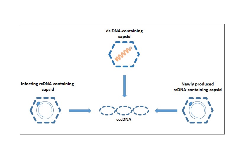
Figure 2: Sources of cccDNA.

4.2 The effects of initial concentration of cccDNA

Upon entering into the nucleus by a partially known mechanism, the partially double-stranded rcDNA is converted into cccDNA. It is thought to be a major factor for persistence of HBV infection as it is resistant to degradation and remains in the nucleus of infected cells even after treatment is completed. Due to the strong stability, cccDNAs are not lost in the course of cell division[50, 51]. It persists in the individuals despite serological evidence of viral clearance. It can also remain in cells for months or even years [35].

In Figure 3, the effects of initial concentration of cccDNA on all components are represented. Five initial concentrations of cccDNA in a small quantity are considered, namely, 20, 40, 60, 80 and 100 unit. Simulations are conducted for a long period of time greater than four years. It is observed that the initial concentrations of cccDNA significantly influence all compartments in the course and outcome of the infection. The presence of a few copies of cccDNA in the liver can re-initiate and blow-up the infection. The small amount of cccDNA that remains in the liver can act as a reservoir for the virus. In contrast, if the antiviral therapy is discontinued or stopped during nearly curable stages of infection, then the viral infection can reactivate. Therefore, while a small amount of cccDNA may not be as clinically significant comparatively a high level of cccDNA, it still represents an important factor in the persistence and transmission of HBV infection.

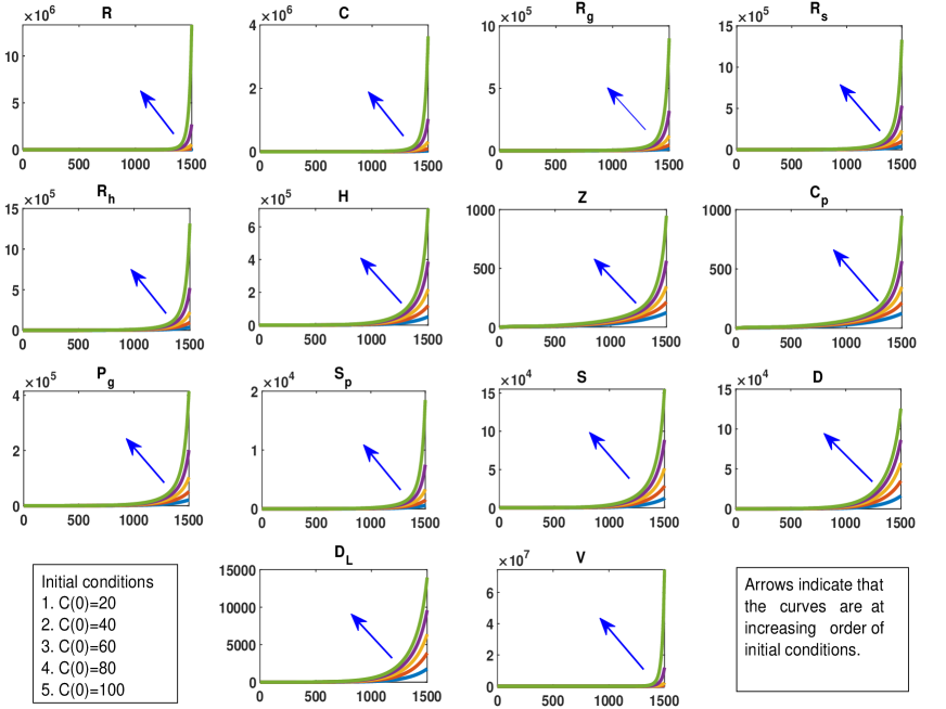
Figure 3: The effects of initial concentrations of cccDNA on all components.

5 Effects of HBx protein ($H$) on HBV infection

HBx plays a critical role in initiating and maintaining HBV replication during the natural infection process [38]. X proteins are able to stimulate de-silencing of cccDNA and prevent the silencing of cccDNA [52]. By inhibiting the development of immune response in HBV infection, HBx protects infected hepatocytes from immune-mediated apoptosis and alters the expression of host genes to facilitate the development of HCC [39]. HBV encodes only the regulatory protein HBx, which involves in multiple aspects of HBV infection. In order to keep cccDNA silent, a novel prospective treatment technique targeting HBx may be proposed. For this purpose, it is included in this model. From the simulation it is seen that the concentration level of cccDNA or concentration level of virus don’t change significantly even after incorporating the effects of HBx in the model. Fatehi et al. [33] also got the similar results from their study. In Figure 4, the effects of HBx proteins on cccDNAs and on viruses are demonstrated. It is seen that the difference between the solutions is not significant. So, targeting the HBx protein as a treatment method in future may not be a promising strategy to control the HBV infection.

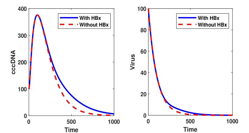
Figure 4: The effects of HBx protein are demonstrated here. Blue solid line represents the solution of the system when the effects of HBx protein are considered. Red dotted line represents the solution of the system when the effects of HBx are not considered.

6 Impacts of intracellular delay ($\tau$)

Time delays play a crucial role in the intracellular replication process of viruses. A delay differential equation (DDE) model has a far more realistic dynamics than an ordinary differential equation. Time delay may be responsible for the loss of stability of a steady state and the oscillations in population dynamics. Two types of delays exist: pharmacological and intracellular. The delay between the ingestion of a drug and its appearance within cells is known as the pharmacological delay. The time elapsed between the infection of a host cell and the discharge of viral particles is known as the intracellular delay. In this study, the intracellular delay, designated by $\tau$, is incorporated into the every step of HBV life cycle to make the process non-instantaneous. The intracellular delay model is given by the equation (19) in Appendix A. The system of delay differential equation (19) is solved numerically for different value of $\tau$. As a result, it is observed that intracellular delay has very little impact on viral dynamics. (results are not shown)

7 Impacts of surface proteins on infection

Although HBx protein and intracellular delay ($\tau$) play some roles in cccDNA production inside the nucleus, these factors are not major contributors to the persistence of HBV infection in the host. Surface proteins (L, M, S), one kind of glycoprotein, also play significance roles in viral synthesis, viral infection, and in induction of immune responses. The primary role of the surface proteins is to allow the virus to bind to the receptors of hepatocytes to enter into the cell. Depending on the concentration level of surface proteins inside the hepatocytes, rcDNA-containing capsids can be recycled to the nucleus to increase the number of cccDNA.

The concentration level of HBsAg in the cytoplasm mainly depends on the production rate of surface protein ($\lambda_{rs}$) from cccDNA. According to Nakabayashi [31], there are two types of replication pattern: arrested and explosive. When the productions of 2.4 kb and 2.1 kb mRNAs dominant the production of 3.5 kb pgRNAs, it is called the “arrested replication” pattern. In this case $\lambda_{rg}<\lambda_{rs}$ is a small quantity. On the contrary, in the explosive replication process, the ratio $\lambda_{rg}>\lambda_{rs}$ becomes small in magnitude. Both cases are considered here to study the contribution of HBsAg in HBV infection in a single hepatocyte. In the arrested replication pattern, $\lambda_{rg}=0.1,\leavevmode\nobreak\ \lambda_{rs}=2$, and in the explosive replication pattern $\lambda_{rg}=2,\leavevmode\nobreak\ \lambda_{rs}=0.1$ are considered for simulation purpose only. In Figure 5, the outcomes of these two cases are demonstrated. A significant change in concentration of all intracellular components except polymerase ($P$) are observed. Viral load in the explosive replication pattern is extremely high compared to that in the arrested replication pattern and the solution becomes stable in an endemic equilibrium state. It is also observed that the explosive replication pattern indicates the chronic infection, whereas arrested replication pattern reflects the acute infection. Therefore, availability of HBsAg in the infected cell may drastically change the amount of newly produced virion from an infected cell as well as the situation of the patient.

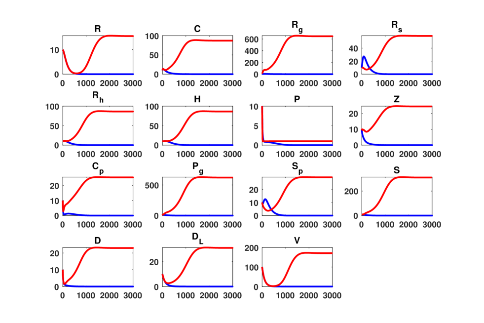
Figure 5: The effects of HBsAg on all intracellular components are demonstrated here. Here, red curve and blue curve represent the outcomes of explosive replication $(\frac{\lambda_{rs}}{\lambda_{rg}}<<1)$ and arrested replication $(\frac{\lambda_{rg}}{\lambda_{rs}}<<1)$ patterns. We take time along the x-axis and concentrations of each component along y-axis.

8 Impacts of double-stranded linear DNA-containing capsids

The impacts of dslDNA-containing capsids on all other intracellular components are discussed here. dslDNA is a defective form of the viral DNA. It can produce surface proteins (L, M, and S), but may not be able to produce functional pgRNA due to some mutations that are introduced when it is converted into cccDNA [53]. In section 3, the roles of dslDNA are incorporated into the model (16) by the parameter $\lambda_{sdl}$. Keeping other parameters fixed, the system (16) is solved for different values of $\lambda_{sdl}$. The outcomes of cccDNA and virus are shown in Figure 6. No substantial change or role is observed within each class (ccDNA and virus). Therefore, targeting the dslDNA containing capsids for possible future treatment options does not seem promising. Moreover, the differential equation corresponding to the dslDNA-containing capsids can be ignored to simplify the model (16) for further analysis.

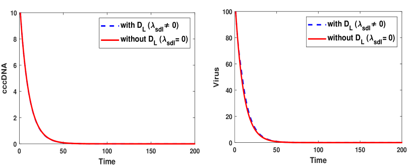
Figure 6: The effects of dslDNA containing capsids on cccDNA and virus compartment are demonstrated here.

9 Global sensitivity analysis of model parameters

Because of uncertainties in experimental data used in the estimation of model parameters, the accuracy of outputs of a mathematical model related to specific biological phenomena becomes frequently poor. Many authors now focus on local sensitivity analysis (LSA), which is the examination of the impacts of one parameter while holding the others fixed at their estimated values. However, LSA does not offer complete necessary information about the uncertainty and sensitivity of the concerned parameter. In this case, global sensitivity analysis (GSA) performs well and can clearly describe the contributions of each model parameter irrespective of the role of other parameters. The GSA is a statistical technique which is used to study the sensitivity of parameters of a system or of a mathematical model. Various methods are used to study the global sensitivity analysis, such as Sobol indices, Fourier amplitude sensitivity test, partial rank correlation coefficient (PRCC). In this study, Latin hypercube sampling-partial rank correlation coefficient (LHS-PRCC) method is applied to the model (17). This method is well-explained in the article of Marino et al. [54]. In this method, PRCC values can provide relevant useful information. PRCC can also aid us in determining the most influential set of parameters for achieving specific objectives in elimination of disease.

9.1 Simplified model

The full dynamics model (16) is simplified for further analysis. In order to do this, some proper assumptions are made here. A similar kind of approach, as mentioned in the article of Nakabayashi [31] is followed here to do the simplification.

1. If the intracellular components are degraded rapidly compared to the recruitment rate, then the infection will disappear on its own. The degradation rates are therefore assumed to be too small and can be ignored.

2. In section 5, it is seen that the effects of HBx protein on infection are not significant. So, equations $\frac{dR_{h}}{dt}=\lambda_{rh}\Phi C-\delta_{r_{h}}R_{h}$ and $\frac{dH}{dt}=\lambda_{h}R_{h}-\delta_{h}H$ are ignored. In this case, the volume fraction of active cccDNA $\Phi(t)$ becomes $\Phi_{0}$. It means that all cccDNAs are active. Therefore, $\Phi_{0}$ is taken to be equal to 1.

3. The system (16) does not seem to be affected by dslDNA-containing capsids, as observed in section 8. Thus, the differential equation corresponding to dlsDNA in full dynamics model (16) is also ignored here.

Therefore, on the basis of these assumptions, the full dynamics model (16) is reduced to the following:

$$\left.\begin{split}\text{rcDNA:}\leavevmode\nobreak\ &\frac{dR}{dt}=\alpha_{1}V-\alpha_{2}R,\\ \text{cccDNA:}\leavevmode\nobreak\ &\frac{dC}{dt}=\alpha_{2}R+k_{1}e^{-\lambda S_{p}}D-\delta_{c}C.\\ \text{3.5\leavevmode\nobreak\ kb\leavevmode\nobreak\ mRNA:}\leavevmode\nobreak\ &\frac{dR_{g}}{dt}=\lambda_{rg}C-\mu_{1}R_{g}P,\\ \text{(2.4+2.1)\leavevmode\nobreak\ kb\leavevmode\nobreak\ mRNA:}\leavevmode\nobreak\ &\frac{dR_{s}}{dt}=\lambda_{rs}C-\lambda_{s_{p}}R_{s},\\ \text{Ploymerase:}\leavevmode\nobreak\ &\frac{dP}{dt}=\lambda_{p}R_{g}-\mu_{1}R_{g}P,\\ \text{RNP complex:}\leavevmode\nobreak\ &\frac{dZ}{dt}=\mu_{1}R_{g}P-\mu_{2}ZC_{p},\\ \text{Core protein:}\leavevmode\nobreak\ &\frac{dC_{p}}{dt}=\lambda_{c}R_{g}-\mu_{2}ZC_{p},\\ \text{pgRNA-containing capsid:}\leavevmode\nobreak\ &\frac{dP_{g}}{dt}=\mu_{2}ZC_{p}-\beta_{1}P_{g}.\\ \text{Surface protein:}\leavevmode\nobreak\ &\frac{dS_{p}}{dt}=\lambda_{s_{p}}R_{s}-\eta_{s_{p}}S_{p},\\ \text{ssDNA-containing capsid:}\leavevmode\nobreak\ &\frac{dS}{dt}=\beta_{1}P_{g}-\beta_{2}S,\\ \text{dsDNA-containing capsid:}\leavevmode\nobreak\ &\frac{dD}{dt}=\beta_{2}S-k_{1}e^{-\lambda S_{p}}D-k_{2}\left(1-e^{-\lambda S_{p}}\right)DS_{p},\\ \text{Virus:}\leavevmode\nobreak\ &\frac{dV}{dt}=k_{2}\left(1-e^{-\lambda S_{p}}\right)DS_{p}-\delta_{v}V,\end{split}\right\}$$ (17)

Table 3: Baseline, maximum and minimum values of parameters used in the global sensitivity analysis.

Parameters	Minimum (50% of baseline value)	Baseline value	Maximum (150% of baseline value)
$\alpha_{1}$	0.015	0.03	0.045
$\alpha_{2}$	0.3465	0.693	1.0395
$k_{1}$	0.3465	0.693	1.0395
$\lambda$	0.000005	0.00001	0.000015
$\delta_{c}$	0.008	0.016	0.024
$\lambda_{rg}$	324	648	972
$\mu_{1}$	60	120	180
$\lambda_{rs}$	450	900	1350
$\lambda_{sp}$	2500	5000	7500
$\lambda_{p}$	270	540	810
$\mu_{2}$	0.3465	0.693	1.0395
$\lambda_{c}$	308.5	617	925.5
$\beta_{1}$	25	50	75
$\eta_{sp}$	50	100	150
$\beta_{2}$	0.3465	0.693	1.0395
$k_{2}$	0.3465	0.693	1.0395
$\delta_{v}$	2.079	4.158	6.237

9.2 Latin hypercube sampling (LHS)-Partial rank correlation coefficient (PRCC)

Latin hypercube sampling is one kind of statistical method, belong to Monte Carlo class. With help of this method, a random sample of parameter values from a multi-dimensional distribution can be generated. This method was introduced in 1979 by McKay et al. [55]. In the context of statistical sampling, sample inputs, basically the parameters of the model are distributed in a “$q$-dimensional hypercube”, where $q$ denotes the number of parameters considered in the proposed model. For our simplified model (17), there are 17 parameters. By partitioning the given ranges of parameters into probable equal sub-intervals, a probability density function (pdf) is employed to sample the parameter values. Sample points are placed in such a way that each should satisfy the LHS requirements. Based on the prior information and existing data, we use the uniform distribution for all parameters in this work. The model is then simulated iteratively over the hypercube. In general, the sample size $N$ be at least $(q+1)$. But, it is suggested that the sample size should be larger to ensure the desired precision and accuracy of the results. In this study, the sample size of 1000 is chosen. The correlation coefficient (CC) serves as a metric to gauge the strength of linear correlation between the inputs and the outputs. The correlation coefficient can be calculated using the following formula:

$${r}=\dfrac{\sum(U-\bar{U})(V-\bar{V})}{\sqrt{\sum(U-\bar{U})^{2}\sum(V-\bar{V})^{2}}},$$

where $U$ and $V$ are inputs and outputs variables, respectively. $\bar{U}$ and $\bar{V}$ represent the sample means of $U$ and $V$, and $r\in[-1,1]$. Depending on the characteristics/nature of the data, the correlation coefficient may be referred to by different alternative names. In case of raw data of $U$ and $V$, the correlation coefficient $(r)$ is called sample or Pearson correlation coefficient. On the other hand, when the data is rank-transformed, the correlation coefficient is defined as the Spearman or rank correlation coefficient. LHS-PRCC provides a powerful tool to understand how the outputs of a system are affected by variations in model parameters. Marino et al. well-described this method in their study [54].

9.3 Scatter plots: The monotonic relationship between input and output variables

In order to make better prediction about the infection and propose a new treatment strategy, it is very essential to explore how the outputs of a system or a model are influenced if the values of the associated parameters are varied within a reasonable range. The baseline values of each parameter are taken from the literature and shown in Table 3. Simulation results of the simplified model (17) are shown by scatter plots in Figure 8-Figure 19. On day 280, PRCC values of all model parameters are computed with respect to dependent variables, and are visualized in Table 4. The positive PRCC value associated with a model parameter and a compartment indicates that any increase or decrease in the parameter’s value, whether individually or simultaneously, leads to an enhancement or reduction in the concentration of the compartment. On the other hand, negative correlation (PRCC value negative) tells us the opposite aspects. The positive and negative correlated parameters for corresponding compartments are shown in second and third columns of Table 5, respectively. Based on the PRCC value, the insignificant or very less significant parameters are also identified and listed those in the fourth column of Table 5. The most positively significant (MPS) and most negatively significant (MNS) parameters for a specific compartment are highlighted in the fifth and sixth columns of the same Table 5.

Global sensitivity analysis reveals several new and striking results. Based on the PRCC values ( Table 4) and outputs noted down in Table 5, some of the findings are listed below.

1. The exit rate of sub-viral particles ($\eta_{sp}$) is positively correlated with almost all except surface proteins i.e. the sub-viral particles play an important role in acceleration and persistence of HBV infection. Sub-viral particles can serve as decoys for the host immune system. These particles circulate in the bloodstream and are recognized by the immune system as foreign particles [56]. The immune response generated against sub-viral particles diverts the attention of immune system away from the infectious viral particles, which allows the virus to persist in the host. Despite being non-infectious, sub-viral particles hold crucial significance in understanding HBV infection due to their direct involvement in the disease progression. Henceforth, these particles hold immense potential for applications in various aspects, including their utilization as diagnostic markers, vaccine development tools, and as a basis for proposing novel therapeutic approaches to combat the disease.

2. The recycling rate ($k_{1}$) is positively correlated with all components except dsDNA-containing capsids. While not being the most significant parameter for any compartment, it plays some versatile roles throughout the infection. Surface protein is the most affected component by recycling rate. All other components are moderately influenced. Therefore, recycling of capsids exerts significant effects on the overall dynamics of the HBV infection.

3. The production rate of 3.5 kb pgRNA ($\lambda_{rg}$) is positively correlated with all compartments which implies that the transcription of cccDNA is one of the key step in the viral life cycle. It is one of the greatest influential parameters in the system. Hence, this parameter will need to be taken into account while proposing any new control strategy.

4. The parameter $\lambda$ is negatively correlated with almost all compartments that means rcDNA transportation rate to the nucleus are highly associated to the cccDNA synthesis within the hepatocytes.

5. The decay rate of cccDNA ($\delta_{c}$) and virus ($\delta_{v}$) are negatively correlated with almost all except dsDNA-containing capsids. It’s also a noteworthy observation.

6. Production rate of 2.4 kb and 2.1 kb mRNA ($\lambda_{rs}$) is negatively correlated with nearly all except 2.4 kb and 2.1 kb mRNAs ($R_{s}$) and surface proteins. This parameter is also the most negatively sensitive parameter for both cccDNA and dsDNA-containing capsids.

7. It is also observed that the production rate of polymerase ($\lambda_{p}$) and the production rate of core proteins ($\lambda_{c}$) both are sensitive (positive for some compartments and negative for others) for all compartments. In addition, these two parameters are synchronously MPS and MNS i.e. as far as the infection is concerned, production rate of polymerase and core proteins play dual role in infection period. It is one of the crucial findings in this study. Probably, dual role of these two parameters are noticed in this study for the first time. No one has informed about this kind of behaviors of parameters so far.

The sensitivity analysis of this intracellular dynamics model helps us in determination of those factors that has immense influence in causing the infection. Although, it might be very difficult to pinpoint the most significant parameter for this infection, but we are able to enlist successfully ten parameters out of thirty-four, which have relatively greater impacts. Considering all these results and findings, it is possible to determine the best way to control this disease and to select the most effective drug regimens. Furthermore, the most beneficial and best suited combination of available drugs (according to their chemical ingredients and maintaining the drug-drug interactions) can be chosen for the patient. In a nutshell, it is expected that this study will be useful in a wide range of practical applications.

9.4 Critical observation

From Table 4, it is observed that PRCC values for the transcription rate ($\lambda_{rg}$) of 3.5 kb pgRNA remain positive for all compartments, whereas the transcription rate of 2.4 and 2.1 kb mRNA $(\lambda_{rs})$ predominantly yield negative PRCC values across nearly all compartments. It is perplexing that when both parameters, associated with transcription, exhibit completely opposite contributions to the infection, which raises questions about their underlying mechanisms. This study provides a clear understanding of this fact. When the value of $\lambda_{rs}$ is low, the production of surface proteins will decrease. As a consequence, a smaller number of rcDNA-containing capsids will be enveloped by surface proteins. On the other hand, a larger number of capsids will generate a higher quantity of cccDNA through the recycling loop. The transcription of this substantial amount of cccDNA will lead to the synthesis of a large quantity of pgRNA and surface proteins. As a result, these series of process will ultimately lead to a significant augmentation/enhancement in the release virus particles. Therefore, it can be concluded that solely focusing on this parameter to decrease the production of surface proteins would not be a viable approach to effectively control the infection.

Table 4: List of PRCC values. As shown in the north-west box, P stands for parameters and V stands for variables. Blue and red cells represent highest and lowest PRCC values of the corresponding component/model variable.

	$R$	$C$	$R_{g}$	$R_{s}$	$P$	$Z$	$C_{p}$	$P_{g}$	$S_{p}$	$S$	$D$	$V$
$\alpha_{1}$	0.7131	0.1215	0.1393	0.0552	-0.0930	0.0215	-0.0073	0.0688	0.1273	0.0543	-0.1016	0.0530
$\alpha_{2}$	-0.7010	-0.0135	-0.0220	-0.0439	-0.0321	0.0057	-0.0016	-0.0100	-0.0194	0.0085	-0.0037	-0.0250
$k_{1}$	0.4193	0.6718	0.5960	0.7087	0.0168	0.0419	0.1800	0.4778	0.7952	0.4969	-0.7067	0.4417
$\lambda$	-0.4600	-0.6975	-0.6049	-0.7059	-0.0080	-0.0956	-0.1084	-0.4710	-0.7973	-0.4978	-0.7109	-0.4437
$\delta_{c}$	-0.5592	-0.7606	-0.6615	-0.7659	-0.0523	-0.1154	-0.1750	-0.5462	-0.8457	-0.5551	0.7069	-0.5506
$\lambda_{rg}$	0.8587	0.7518	0.9252	0.7740	0.0186	0.2506	0.4345	0.8683	0.8427	0.8730	0.7120	0.8627
$\mu_{1}$	-0.0803	-0.0735	-0.1054	-0.0830	-0.9667	-0.0009	-0.0276	-0.0789	-0.0576	-0.0875	-0.0825	-0.0828
$\lambda_{rs}$	-0.5741	-0.7814	-0.7013	0.0319	-0.0554	-0.1657	-0.1599	-0.5837	0.0222	-0.5993	-0.8171	-0.5737
$\lambda_{sp}$	-0.0406	-0.0268	-0.0220	-0.8961	0.0482	-0.0368	0.0313	-0.0159	-0.0368	-0.0272	-0.0351	-0.0239
$\lambda_{p}$	-0.4714	-0.3586	-0.8754	-0.3802	0.9655	0.9113	-0.9139	-0.4832	-0.4482	-0.4723	-0.3069	-0.4570
$\mu_{2}$	0.0151	-0.0082	-0.0383	0.0016	0.0098	-0.3019	-0.1509	0.0072	-0.0158	0.0187	0.0039	0.0194
$\lambda_{c}$	0.5824	0.4372	0.3284	0.4460	-0.0013	-0.9119	0.9172	0.5662	0.5655	0.5779	0.3955	0.5777
$\beta_{1}$	0.0381	0.0348	0.0156	0.0520	0.0224	-0.0137	0.0468	-0.7124	0.0176	0.0540	0.0282	0.0329
$\eta_{sp}$	0.7082	0.8879	0.8250	0.8939	0.0356	0.1382	0.3302	0.7282	-0.0238	0.7483	0.9037	0.7109
$\beta_{2}$	0.0390	-0.0242	-0.0244	-0.0271	0.0136	-0.0340	0.0413	-0.0105	-0.0153	-0.7475	-0.0024	0.0038
$k_{2}$	-0.4546	-0.6877	-0.6195	-0.7057	0.0264	-0.0389	-0.2164	-0.5092	-0.7994	-0.5136	-0.7396	-0.4775
$\delta_{v}$	-0.7290	-0.1298	-0.0687	-0.1556	-0.0031	-0.0007	-0.0493	-0.0842	-0.1326	-0.1003	0.0554	-0.7426

Table 5: Complete list of positively correlated, negatively correlated, non-significant, most positively significant and most negatively significant parameters. The parameters that are positively correlated are arranged in monotonically decreasing order whereas those that are negatively correlated are arranged in monotonically increasing order so that one can easily identify the parameters in the sequence: most significant, second most significant and so on.

Variables	Positively correlated parameters	Negatively correlated parameters	Insensitive parameters	Most positively sensitive parameter	Most negatively sensitive parameter
$R$	$\lambda_{rg},\leavevmode\nobreak\ \alpha_{1},\leavevmode\nobreak\ \eta_{sp}$	$\delta_{v},\leavevmode\nobreak\ \alpha_{2},\leavevmode\nobreak\ \lambda_{rs},\leavevmode\nobreak\ \delta_{c},$	$\mu_{1},\leavevmode\nobreak\ \lambda_{sp},\leavevmode\nobreak\ \mu_{2},$	$\pagecolor{blue!20}\lambda_{rg}$	$\delta_{v}$
	$\lambda_{c},\leavevmode\nobreak\ k_{1}$	$\lambda_{p},\leavevmode\nobreak\ k_{2},\leavevmode\nobreak\ \lambda$	$\beta_{1},\leavevmode\nobreak\ \beta_{2}$
$C$	$\eta_{sp},\leavevmode\nobreak\ \lambda_{rg},$	$\lambda_{rs},\leavevmode\nobreak\ \delta_{c},\leavevmode\nobreak\ \lambda,$	$\alpha_{1},\leavevmode\nobreak\ \alpha_{2},\leavevmode\nobreak\ \lambda_{sp},\leavevmode\nobreak\ \beta_{1},$	$\pagecolor{red!40}\eta_{sp}$	$\lambda_{rs}$
	$k_{1},\leavevmode\nobreak\ \lambda_{c}$	$k_{2},\leavevmode\nobreak\ \lambda_{p},\leavevmode\nobreak\ \mu_{1}$	$\eta_{sp},\leavevmode\nobreak\ \beta_{2},\leavevmode\nobreak\ \delta_{v}$
$R_{g}$	$\lambda_{rg},\leavevmode\nobreak\ \eta_{sp},$	$\lambda_{p},\leavevmode\nobreak\ \lambda_{rs},\leavevmode\nobreak\ \delta_{c},$	$\alpha_{1},\leavevmode\nobreak\ \alpha_{2},\mu_{1},\leavevmode\nobreak\ \mu_{2},$	$\pagecolor{blue!20}\lambda_{rg}$	$\lambda_{p}$
	$k_{1},\leavevmode\nobreak\ \lambda_{c}$	$k_{2},\leavevmode\nobreak\ \lambda$	$\lambda_{sp},\leavevmode\nobreak\ \beta_{1},\leavevmode\nobreak\ \beta_{2},\leavevmode\nobreak\ \delta_{v}$
$R_{s}$	$\eta_{sp},\leavevmode\nobreak\ \lambda_{rg},$	$\lambda_{sp},\leavevmode\nobreak\ \delta_{c},\leavevmode\nobreak\ \lambda,$	$\alpha_{1},\leavevmode\nobreak\ \alpha_{2},\mu_{1},\leavevmode\nobreak\ \mu_{2},\leavevmode\nobreak\ \lambda_{rs},$	$\pagecolor{red!40}\eta_{sp}$	$\lambda_{sp}$
	$k_{1}$	$k_{2},\leavevmode\nobreak\ \lambda_{p}$	$\lambda_{c},\leavevmode\nobreak\ \beta_{1},\leavevmode\nobreak\ \beta_{2},\leavevmode\nobreak\ \delta_{v}$
$P$	$\lambda_{p}$	$\mu_{1}$	All other parameters	$\lambda_{p}$	$\mu_{1}$
$C_{p}$	$\lambda_{c},\leavevmode\nobreak\ \eta_{sp}$	$\lambda_{p},\leavevmode\nobreak\ \lambda_{rg}$	All other parameters	$\lambda_{c}$	$\lambda_{p}$
$Z$	$\lambda_{p}$	$\lambda_{c},\leavevmode\nobreak\ \mu_{2}$	All other parameters	$\lambda_{p}$	$\lambda_{c}$
$P_{g}$	$\lambda_{rg},\leavevmode\nobreak\ \eta_{sp},$	$\beta_{1},\leavevmode\nobreak\ \lambda_{rs},\leavevmode\nobreak\ \delta_{c},$	$\alpha_{1},\leavevmode\nobreak\ \alpha_{2},\mu_{1},\leavevmode\nobreak\ \mu_{2},$	$\pagecolor{blue!20}\lambda_{rg}$	$\beta_{1}$
	$\lambda_{c},\leavevmode\nobreak\ k_{1}$	$k_{2},\leavevmode\nobreak\ \lambda_{p},\leavevmode\nobreak\ \lambda$	$\lambda_{sp},\leavevmode\nobreak\ \beta_{2},\leavevmode\nobreak\ \delta_{v}$
$S_{p}$	$\lambda_{rg},\leavevmode\nobreak\ k_{1},$	$\delta_{c},\leavevmode\nobreak\ k_{2},$	All other	$\pagecolor{blue!20}\lambda_{rg}$	$\delta_{c}$
	$\lambda_{c}$	$\lambda,\leavevmode\nobreak\ \lambda_{p}$	parameters
$S$	$\lambda_{rg},\leavevmode\nobreak\ \eta_{sp},$	$\beta_{2},\lambda_{rs},\leavevmode\nobreak\ \delta_{c},$	All other	$\pagecolor{blue!20}\lambda_{rg}$	$\beta_{2}$
	$\lambda_{c},\leavevmode\nobreak\ k_{1}$	$\lambda,\leavevmode\nobreak\ \lambda_{p}$	parameters
$D$	$\eta_{sp},\leavevmode\nobreak\ \lambda_{rg},$	$\lambda_{rs},\leavevmode\nobreak\ \lambda,$	All other	$\pagecolor{red!40}\eta_{sp}$	$\lambda_{rs}$
	$\delta_{c}$	$k_{1},\leavevmode\nobreak\ \lambda_{p}$	parameters
$V$	$\lambda_{rg},\leavevmode\nobreak\ \eta_{sp},$	$\delta_{v},\leavevmode\nobreak\ \lambda_{rs},\leavevmode\nobreak\ \delta_{c},$	All other	$\pagecolor{blue!20}\lambda_{rg}$	$\delta_{v}$
	$\lambda_{c},\leavevmode\nobreak\ k_{1}$	$k_{2},\leavevmode\nobreak\ \lambda_{p},\leavevmode\nobreak\ \lambda$	parameters

10 Model validation

In order to validate the proposed model, the simplified model (17) is extended incorporating the effects of entecavir (ETV), which acts as a reverse transcriptase inhibitor $i.e.$ it blocks the production of dsDNA-containing capsids from pgRNA-containing capsids. It is assumed that the efficiency of ETV is $\epsilon$, where $0<\epsilon\leq 1$. As a result of incorporation of ETV, equation (10) and equation (11) are modified as follows:

$$\left.\begin{split}&\frac{dP_{g}}{dt}=\mu_{2}ZC_{p}-(1-\epsilon)\beta_{1}P_{g},\\ &\frac{dS}{dt}=(1-\epsilon)\beta_{1}P_{g}-\beta_{2}S.\\ \end{split}\right\}$$ (18)

Experimental data of four humanized mice are collected from the work of Kitagawa et al. [57]. Each mouse was infected with HBV at $1.0\times 10^{6}$copies. On the day 53 of post-inoculation, the mice, displaying a sustained level of HBV in serum, were administered ETV continuously for 70 days. The treatment protocol involved daily dosing of 0.02 mg/kg ETV. The efficiency of ETV, as stated in the study by Kitagawa et al. [57], is recorded as 0.97, and this value is utilized in our study. Through a thorough comparison between the model solution and the experimental data from four humanized mice (Mouse-501, Mouse-502, Mouse-503, Mouse-504), it is seen from Figure 7 that the model well-captured the experimental data as well dynamics of infection. Therefore, the model demonstrates a close alignment with reality and reflects a strong correspondence with actual observations. In Figure 7, the comparisons are visualized.

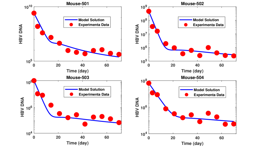
Figure 7: Dynamics HBV-infected humanized mice. The proposed model is calibrated using experimental data collected from humanized mice subjected to ETV treatment.

11 Conclusions

In case of viral infection, intracellular dynamics model has revealed various intrinsic biological phenomena of individual cells. Considering all possible steps of the HBV life cycle, this study proposes an intracellular dynamics model. To the best of our knowledge, it is the most generalized and reasonable dynamics model yet. A detailed discussion of nearly all possible viral replication mechanisms is provided here. Large number of parameters (comparatively existing study in the literature) have been handled successfully and their roles in disease progression and persistence are explored. The proposed intracellular dynamics model is validated with experimental data obtained from humanized mice.

The evaluation of uncertainties and sensitivity analysis has gained importance in assessing the reliability of models and identifying the most influential factors on outputs. In order to study the sensitivity of the model’s parameters, a sampling-based method (Latin hypercube sampling-Partial Rank Correlation Coefficient) is used here. The most positively and negatively correlated parameters for a specific compartment and for the entire system are identified. It is also uncovered that some parameters have a dual role in modulating disease dynamics.

Based on the findings of the present study, the following conclusions can be drawn:

1. There is no significant contribution of HBx proteins to the progression of HBV infection. So, targeting the HBx protein as a future antiviral therapy is not a promising strategy to control the infection.

2. Superinfection of cells can lead to more severe liver damage and increase risk of complications. cccDNA and progeny viruses are highly amplified in the presence of superinfection. In a nutshell, superinfection rate is one of the disease controlling parameters.

3. The simulation results illustrate that the intracellular delay has little effects on the infection.

4. HBsAg is one of the main viral components. The availability of HBsAg in the infected cell switches the arrested replication pattern to explosive replication and vice versa. Therefore, considering other factors, it may be worthwhile to inhibit all the functions of HBsAg to treat HBV patients.

5. This study indicates that dslDNA has no bearing on the outcomes of infection.

6. During recycling of capsids, core particles assemble inside infected cells and serve as a source of infection. In other word, the recycling of capsids serves as a positive feedback loop in the infection. The available inhibitors associated with capsids recycling mechanism have proved to be effective at reducing HBV infection.

7. The results of the global sensitivity analysis indicate that the parameters related to transcription ($\lambda_{rg}$), translation ($\lambda_{p},\leavevmode\nobreak\ \lambda_{c}$) and exit of sub-viral particles ($\eta_{sp}$) have more substantial impacts on disease development compared to other parameters.

However, these findings represent the tip of the iceberg, and deeper mechanisms must be uncovered. The outcomes of this study will advance the understanding of infection clearance and may be applied in practical field including the clinical experiments. We aim to enhance our current model by including all existing antiviral therapy in the near future. Our main focus is to identify the optimal monotherapy or combination therapy based on the individual patient’s overall condition.

Acknowledgments

First author would like to acknowledge the financial support obtained from CSIR (New Delhi) under the CSIR-SRF Fellowship scheme (File No: 09/731(0171)/2019-EMR-I). The first author also thanks the research facilities received from the Department of Mathematics, Indian Institute of Technology Guwahati, India.

Author contributions

Both authors contribute equally.

Conflict of interest

The authors declare no potential conflict of interests.

Data Availability Statement

Data sharing is not applicable to this article.

Figure 8: Scatter plot for rcDNA ($R$).

  Figure 9: Scatter plot for cccDNA ($C$).

  Figure 10: Scatter plot for 3.5 kb pgRNA ($R_{g}$).

  Figure 11: Scatter plot for 2.4 and 2.1 kb mRNA ($R_{s}$).

  Figure 12: Scatter plot for polymerase ($P$).

  Figure 13: Scatter plot for core protein ($C_{p}$).

  Figure 14: Scatter plot for RNP complex ($Z$).

Figure 15: Scatter plot for pgRNA-containing capsids ($P_{g}$).

  Figure 16: Scatter plot for surface protein ($S_{p}$).

  Figure 17: Scatter plot for single-stranded DNA-containing capsid ($S$).

  Figure 18: Scatter plot for double-stranded DNA-containing capsid ($D$).

  Figure 19: Scatter plot for virus ($V$).

Appendix A

The delay single cell HBV dynamics model is given by

$$\begin{split}&\frac{dR}{dt}=\alpha_{1}V(t-\tau)-\alpha_{2}R-\delta_{r}R.\\ &\frac{dC}{dt}=\alpha_{2}R(t-\tau)+k_{1}e^{-\lambda S_{p}(t-\tau)}D(t-\tau)-\delta_{c}C.\\ &\frac{dR_{g}}{dt}=\lambda_{rg}\Phi C(t-\tau)-\mu_{1}R_{g}P(t-\tau)-\delta_{r_{g}}R_{g},\\ &\frac{dR_{s}}{dt}=\lambda_{rs}\Phi C(t-\tau)+\lambda_{sdl}D_{L}(t-\tau)-\lambda_{s_{p}}R_{s}-\delta_{r_{s}}R_{s},\\ &\frac{dR_{h}}{dt}=\lambda_{rh}\Phi C(t-\tau)-\delta_{r_{h}}R_{h},\\ &\frac{dH}{dt}=\lambda_{h}R_{h}(t-\tau)-\delta_{h}H,\\ &\frac{dP}{dt}=\lambda_{p}R_{g}(t-\tau)-\mu_{1}R_{g}(t-\tau)P-\delta_{p}P,\\ &\frac{dZ}{dt}=\mu_{1}R_{g}(t-\tau)P(t-\tau)-\mu_{2}ZC_{p}(t-\tau)-\delta_{z}Z,\\ &\frac{dC_{p}}{dt}=\lambda_{c}R_{g}(t-\tau)-\mu_{2}Z(t-\tau)C_{p}-\delta_{c_{p}}C_{p},\\ &\frac{dP_{g}}{dt}=\mu_{2}Z(t-\tau)C_{p}(t-\tau)-\delta_{p_{g}}P_{g}.\\ &\frac{dS_{p}}{dt}=\lambda_{s_{p}}R_{s}(t-\tau)-\eta_{s_{p}}S_{p}-\delta_{s_{p}}S_{p},\\ &\frac{dS}{dt}=\beta_{1}P_{g}(t-\tau)-\beta_{2}S-\delta_{s}S,\\ &\frac{dD}{dt}=0.9\beta_{2}S(t-\tau)-k_{1}e^{-\lambda S_{p}}D-k_{2}\left(1-e^{-\lambda S_{p}}\right)DS_{p}-\delta_{d}D,\\ &\frac{dD_{L}}{dt}=0.1\beta_{2}S(t-\tau)-\delta_{d_{L}}D_{L},\\ &\frac{dV}{dt}=k_{2}\left(1-e^{-\lambda S_{p}(t-\tau)}\right)D(t-\tau)S_{p}(t-\tau)-\delta_{v}V,\\ \end{split}$$ (19)

where $\tau$ represents the intracellular delay.

References

- [1] Hepatitis b. https://www.who.int/news-room/fact-sheets/detail/hepatitis-b. 27 July 2021.
- [2] Hepatitis b. https://www.hepb.org/what-is-hepatitis-b/what-is-hepb/facts-and-figures. 2022.
- [3] Jules L Dienstag. Hepatitis b virus infection. New England Journal of Medicine, 359(14):1486–1500, 2008.
- [4] Y Liang, J Jiang, M Su, Z Liu, W Guo, X Huang, R Xie, S Ge, J Hu, Z Jiang, et al. Predictors of relapse in chronic hepatitis b after discontinuation of anti-viral therapy. Alimentary pharmacology & therapeutics, 34(3):344–352, 2011.
- [5] Fabien Zoulim. New insight on hepatitis b virus persistence from the study of intrahepatic viral cccdna. Journal of hepatology, 42(3):302–308, 2005.
- [6] Chee-Kin Hui and George KK Lau. Immune system and hepatitis b virus infection. Journal of Clinical Virology, 34:S44–S48, 2005.
- [7] Stanca M Ciupe, Ruy M Ribeiro, Patrick W Nelson, and Alan S Perelson. Modeling the mechanisms of acute hepatitis b virus infection. Journal of Theoretical Biology, 247(1):23–35, 2007.
- [8] Lequan Min, Yongmei Su, and Yang Kuang. Mathematical analysis of a basic virus infection model with application to hbv infection. The Rocky Mountain Journal of Mathematics, pages 1573–1585, 2008.
- [9] Sanhong Liu and Ran Zhang. On an age-structured hepatitis b virus infection model with hbv dna-containing capsids. Bulletin of the Malaysian Mathematical Sciences Society, 44(3):1345–1370, 2021.
- [10] Arjun Raj, Scott A Rifkin, Erik Andersen, and Alexander Van Oudenaarden. Variability in gene expression underlies incomplete penetrance. Nature, 463(7283):913–918, 2010.
- [11] Ariel A Cohen, Naama Geva-Zatorsky, Eran Eden, Milana Frenkel-Morgenstern, Iirina Issaeva, Alex Sigal, Ron Milo, Cellina Cohen-Saidon, Yuvalal Liron, Zvi Kam, et al. Dynamic proteomics of individual cancer cells in response to a drug. science, 322(5907):1511–1516, 2008.
- [12] Nicholas Navin, Jude Kendall, Jennifer Troge, Peter Andrews, Linda Rodgers, Jeanne McIndoo, Kerry Cook, Asya Stepansky, Dan Levy, Diane Esposito, et al. Tumour evolution inferred by single-cell sequencing. Nature, 472(7341):90–94, 2011.
- [13] M Delbrück. The burst size distribution in the growth of bacterial viruses (bacteriophages). Journal of bacteriology, 50(2):131–135, 1945.
- [14] Thomas Schumann, Helmut Hotzel, Peter Otto, and Reimar Johne. Evidence of interspecies transmission and reassortment among avian group a rotaviruses. Virology, 386(2):334–343, 2009.
- [15] Andrea Timm and John Yin. Kinetics of virus production from single cells. Virology, 424(1):11–17, 2012.
- [16] Michael B Schulte and Raul Andino. Single-cell analysis uncovers extensive biological noise in poliovirus replication. Journal of virology, 88(11):6205–6212, 2014.
- [17] Frank S Heldt, Sascha Y Kupke, Sebastian Dorl, Udo Reichl, and Timo Frensing. Single-cell analysis and stochastic modelling unveil large cell-to-cell variability in influenza a virus infection. Nature communications, 6(1):1–12, 2015.
- [18] Xiu Xin, Hailong Wang, Lingling Han, Mingzhen Wang, Hui Fang, Yao Hao, Jiadai Li, Hu Zhang, Congyi Zheng, and Chao Shen. Single-cell analysis of the impact of host cell heterogeneity on infection with foot-and-mouth disease virus. Journal of virology, 92(9):e00179–18, 2018.
- [19] Ying Zhu, Andrew Yongky, and John Yin. Growth of an rna virus in single cells reveals a broad fitness distribution. Virology, 385(1):39–46, 2009.
- [20] Sara Cristinelli and Angela Ciuffi. The use of single-cell rna-seq to understand virus–host interactions. Current opinion in virology, 29:39–50, 2018.
- [21] Mario L Suvà and Itay Tirosh. Single-cell rna sequencing in cancer: lessons learned and emerging challenges. Molecular cell, 75(1):7–12, 2019.
- [22] Christopher Andrew Tibbitt, Julian Mario Stark, Liesbet Martens, Junjie Ma, Jeff Eron Mold, Kim Deswarte, Ganna Oliynyk, Xiaogang Feng, Bart Norbert Lambrecht, Pieter De Bleser, et al. Single-cell rna sequencing of the t helper cell response to house dust mites defines a distinct gene expression signature in airway th2 cells. Immunity, 51(1):169–184, 2019.
- [23] Yang Zhou, Ziqing Liu, Joshua D Welch, Xu Gao, Li Wang, Tiffany Garbutt, Benjamin Keepers, Hong Ma, Jan F Prins, Weining Shen, et al. Single-cell transcriptomic analyses of cell fate transitions during human cardiac reprogramming. Cell Stem Cell, 25(1):149–164, 2019.
- [24] Corey Saraceni and John Birk. A review of hepatitis b virus and hepatitis c virus immunopathogenesis. Journal of Clinical and Translational Hepatology, (000):0–0, 2021.
- [25] Georgia-Myrto Prifti, Dimitrios Moianos, Erofili Giannakopoulou, Vasiliki Pardali, John E Tavis, and Grigoris Zoidis. Recent advances in hepatitis b treatment. Pharmaceuticals, 14(5):417, 2021.
- [26] Ashish Goyal and Ranjit Chauhan. The dynamics of integration, viral suppression and cell-cell transmission in the development of occult hepatitis b virus infection. Journal of Theoretical Biology, 455:269–280, 2018.
- [27] Martin A Nowak, Sebastian Bonhoeffer, Andrew M Hill, Richard Boehme, Howard C Thomas, and Hugh McDade. Viral dynamics in hepatitis b virus infection. Proceedings of the National Academy of Sciences, 93(9):4398–4402, 1996.
- [28] Anthony Tan, Sarene Koh, and Antonio Bertoletti. Immune response in hepatitis b virus infection. Cold Spring Harbor perspectives in medicine, 5(8):a021428, 2015.
- [29] John M Murray and Ashish Goyal. In silico single cell dynamics of hepatitis b virus infection and clearance. Journal of Theoretical Biology, 366:91–102, 2015.
- [30] F Fatehi Chenar, YN Kyrychko, and KB Blyuss. Mathematical model of immune response to hepatitis b. Journal of Theoretical Biology, 447:98–110, 2018.
- [31] Jun Nakabayashi. The intracellular dynamics of hepatitis b virus (hbv) replication with reproduced virion “re-cycling”. Journal of Theoretical Biology, 396:154–162, 2016.
- [32] Ting Guo, Haihong Liu, Chenglin Xu, and Fang Yan. Global stability of a diffusive and delayed hbv infection model with hbv dna-containing capsids and general incidence rate. Discrete & Continuous Dynamical Systems-B, 23(10):4223, 2018.
- [33] Farzad Fatehi, Richard J Bingham, Eric C Dykeman, Nikesh Patel, Peter G Stockley, and Reidun Twarock. An intracellular model of hepatitis b viral infection: An in silico platform for comparing therapeutic strategies. Viruses, 13(1):11, 2021.
- [34] T Jake Liang. Hepatitis b: the virus and disease. Hepatology, 49(S5):S13–S21, 2009.
- [35] Clara Balsano and Anna Alisi. Viral hepatitis b: established and emerging therapies. Current medicinal chemistry, 15(9):930–939, 2008.
- [36] R Jason Lamontagne, Sumedha Bagga, and Michael J Bouchard. Hepatitis b virus molecular biology and pathogenesis. Hepatoma research, 2:163, 2016.
- [37] Adrien Decorsière, Henrik Mueller, Pieter C Van Breugel, Fabien Abdul, Laetitia Gerossier, Rudolf K Beran, Christine M Livingston, Congrong Niu, Simon P Fletcher, Olivier Hantz, et al. Hepatitis b virus x protein identifies the smc5/6 complex as a host restriction factor. Nature, 531(7594):386–389, 2016.
- [38] Julie Lucifora, Silke Arzberger, David Durantel, Laura Belloni, Michel Strubin, Massimo Levrero, Fabien Zoulim, Olivier Hantz, and Ulrike Protzer. Hepatitis b virus x protein is essential to initiate and maintain virus replication after infection. Journal of hepatology, 55(5):996–1003, 2011.
- [39] Mark A Feitelson, Barbara Bonamassa, and Alla Arzumanyan. The roles of hepatitis b virus-encoded x protein in virus replication and the pathogenesis of chronic liver disease. Expert Opinion on Therapeutic Targets, 18(3):293–306, 2014.
- [40] Thomas Tu, Magdalena A Budzinska, Nicholas A Shackel, and Stephan Urban. Hbv dna integration: molecular mechanisms and clinical implications. Viruses, 9(4):75, 2017.
- [41] Chunkyu Ko, Anindita Chakraborty, Wen-Min Chou, Julia Hasreiter, Jochen M Wettengel, Daniela Stadler, Romina Bester, Theresa Asen, Ke Zhang, Karin Wisskirchen, et al. Hepatitis b virus genome recycling and de novo secondary infection events maintain stable cccdna levels. Journal of hepatology, 69(6):1231–1241, 2018.
- [42] Chunxiao Xu, Haitao Guo, Xiao-Ben Pan, Richeng Mao, Wenquan Yu, Xiaodong Xu, Lai Wei, Jinhong Chang, Timothy M Block, and Ju-Tao Guo. Interferons accelerate decay of replication-competent nucleocapsids of hepatitis b virus. Journal of virology, 84(18):9332–9340, 2010.
- [43] Katrina A Lythgoe, Sheila F Lumley, Lorenzo Pellis, Jane A McKeating, and Philippa C Matthews. Estimating hepatitis b virus cccdna persistence in chronic infection. Virus evolution, 7(1):veaa063, 2021.
- [44] Lidan Hou, Jie Zhao, Shaobing Gao, Tong Ji, Tianyu Song, Yining Li, Jingjie Wang, Chenlu Geng, Min Long, Jiang Chen, et al. Restriction of hepatitis b virus replication by c-abl–induced proteasomal degradation of the viral polymerase. Science advances, 5(2):eaau7130, 2019.
- [45] Rohit Loomba, Martin Decaris, Kelvin W Li, Mahalakshmi Shankaran, Hussein Mohammed, Marcy Matthews, Lisa M Richards, Phirum Nguyen, Emily Rizo, Barbara Andrews, et al. Discovery of half-life of circulating hepatitis b surface antigen in patients with chronic hepatitis b infection using heavy water labeling. Clinical Infectious Diseases, 69(3):542–545, 2019.
- [46] John M Murray, Robert H Purcell, and Stefan F Wieland. The half-life of hepatitis b virions. Hepatology, 44(5):1117–1121, 2006.
- [47] Sabrina Schreiner and Michael Nassal. A role for the host dna damage response in hepatitis b virus cccdna formation—and beyond? Viruses, 9(5):125, 2017.
- [48] Haitao Guo, Chunxiao Xu, Tianlun Zhou, Timothy M Block, and Ju-Tao Guo. Characterization of the host factors required for hepadnavirus covalently closed circular (ccc) dna formation. PLOS ONE, 7(8), 2012.
- [49] Wengang Yang and Jesse Summers. Infection of ducklings with virus particles containing linear double-stranded duck hepatitis b virus dna: illegitimate replication and reversion. Journal of virology, 72(11):8710–8717, 1998.
- [50] Stephen Locarnini. Molecular virology of hepatitis b virus. In Seminars in liver disease, volume 24, pages 3–10. Copyright© 2004 by Thieme Medical Publishers, Inc., 333 Seventh Avenue, New …, 2004.
- [51] Dieter Glebe. Recent advances in hepatitis b virus research: a german point of view. World Journal of Gastroenterology: WJG, 13(1):8, 2007.
- [52] Michael Nassal. Hbv cccdna: viral persistence reservoir and key obstacle for a cure of chronic hepatitis b. Gut, 64(12):1972–1984, 2015.
- [53] Thomas Tu, Henrik Zhang, and Stephan Urban. Hepatitis b virus dna integration: in vitro models for investigating viral pathogenesis and persistence. Viruses, 13(2):180, 2021.
- [54] Simeone Marino, Ian B Hogue, Christian J Ray, and Denise E Kirschner. A methodology for performing global uncertainty and sensitivity analysis in systems biology. Journal of theoretical biology, 254(1):178–196, 2008.
- [55] R. J. Beckman McKay, M. D. and W. J. Conover. A comparison of three methods for selecting values of input variables in the analysis of output from a computer code. Technometrics, 21(2):239–245, 1979.
- [56] Hye Won Lee, Jae Seung Lee, and Sang Hoon Ahn. Hepatitis b virus cure: targets and future therapies. International journal of molecular sciences, 22(1):213, 2020.
- [57] Kosaku Kitagawa, Kwang Su Kim, Masashi Iwamoto, Sanae Hayashi, Hyeongki Park, Takara Nishiyama, Naotoshi Nakamura, Yasuhisa Fujita, Shinji Nakaoka, Kazuyuki Aihara, Alan Perelson, Lena Allweiss, Maura Dandri, Koichi Watashi, Yasuhito Tanaka, and Shingo Iwami. Multiscale modeling of hbv infection integrating intra- and intercellular viral propagation for analyzing extracellular viral markers, 2023.