Bundle-specific Tractogram Distribution Estimation Using Higher-order Streamline Differential Equation

Abstract

Tractography traces the peak directions extracted from fiber orientation distribution (FOD) suffering from ambiguous spatial correspondences between diffusion directions and fiber geometry, which is prone to producing erroneous tracks while missing true positive connections. The peaks-based tractography methods “locally” reconstructed streamlines in ‘single to single’ manner, thus lacking of global information about the trend of the whole fiber bundle. In this work, we propose a novel tractography method based on a bundle-specific tractogram distribution function by using a higher-order streamline differential equation, which reconstructs the streamline bundles in ‘cluster to cluster’ manner. A unified framework for any higher-order streamline differential equation is presented to describe the fiber bundles with disjoint streamlines defined based on the diffusion tensor vector field. At the global level, the tractography process is simplified as the estimation of bundle-specific tractogram distribution (BTD) coefficients by minimizing the energy optimization model, and is used to characterize the relations between BTD and diffusion tensor vector under the prior guidance by introducing the tractogram bundle information to provide anatomic priors. Experiments are performed on simulated Hough, Sine, Circle data, ISMRM 2015 Tractography Challenge data, FiberCup data, and in vivo data from the Human Connectome Project (HCP) data for qualitative and quantitative evaluation. The results demonstrate that our approach can reconstruct the complex global fiber bundles directly. BTD reduces the error deviation and accumulation at the local level and shows better results in reconstructing long-range, twisting, and large fanning tracts.

Diffusion MRI, Tractography, Bundle-specific tractography distribution, High-order streamline differential equation.

1 Introduction

TRACTOGRAPHY based on diffusion weighted magnetic resonance imaging (dMRI) is a potentially useful way of revealing the trajectories of white matter and structural connectome of the human brain in vivo [1, 2, 3, 4]. Typically, conventional tractography aims to integrate voxel-scale local fiber orientation extracted from fiber orientation distribution (FOD) to infer global connectivity, called FOD-based tractography [5], which faces challenges of producing large amounts of false-positives fibers and omitting true-positives fibers. These challenges have been widely discussed in schematic representations or theoretical arguments [6, 7, 8]. In general, it is usually attributed to the spatially ambiguous correspondences between diffusion directions and fiber geometry on voxel, local and global levels [1, 9, 10].

In recent decades, numerous efforts have been devoted to accurately estimating fiber trajectories, which are mainly reflected in diffusion modeling techniques and tractography strategies. For the diffusion modeling, high angular resolution diffusion imaging (HARDIs), such as constrained spherical deconvolution [11] and high-order tensor [12], are proposed to characterize multiple fibers within one voxel to overcome the limitation of DTI model. However, diffusion orientations are ambiguous when the asymmetric curvatures of the underlying fiber bundles are in the range of the voxel size [13, 3].

In recent years, asymmetric fiber orientation distributions (AFODs) have been proposed to address the problem of asymmetric fiber geometry. S. N. Sotiropoulos et al. [14] estimated fiber dispersion using Bingham distributions to represent continuous distributions of fiber orientations, centered on the main orientation, and captured anisotropic dispersion. Based on the geometric interpretation, Reisert et al. [15] derived a continuity condition that should be preserved for valid AFODs. Cetin et al. [13] proposed an asymmetric orientation distribution function (ODF) using a cone model in a voxel-wise manner. Considering the local surroundings of a voxel and using intervoxel information to derive potential fiber patterns is another approach used to estimating fiber geometry [16, 17, 18]. For instance, the estimation of AFODs based on a spherical deconvolution approach uses a set of symmetric and asymmetric basis functions by adding neighborhood continuity components [16]. However, these asymmetric models are good at representing such specific fiber geometry and simply plugging these AFODs into a typical tractography paradigm continues to face ambiguous spatial correspondences. Voxel-level or local-level diffusion models face challenges in resolving global fiber trajectory reconstruction with complex tractograms.

For tractography strategies, current tractography methods are based on the peaks extracted from FODs or AFODs, which we named peak-based tractography. Typical deterministic tractography tracks the peaks of the maximum diffusion direction, which inevitably accumulates error in the process. The probabilistic tractography algorithm obtains the fibers by randomly extracting directions from the FOD, leading to the production of substantial amounts of false-positive fibers [19, 20, 21, 22, 23]. Filter-based tractography [24, 25] can optimize the signal prediction error to iteratively reduce tractography biases when tracing the maximum diffusion direction. The signal is examined at each new position, and the filter recursively updates the underlying local model parameters to indicate the direction in which to propagate tractography. Filter-based methods cannot capture global fiber trajectory information to guide filtering and only optimize the fiber trajectory at the local level. Global optimization based tractography approaches [26, 27, 28, 29, 30, 31] reconstruct the fiber pathways, which aim to maximize the global energy of the vector field and the fiber structure solutions to prevent the fiber trajectory from being affected by local fiber direction errors. However, they can always find the maximal energy path between two seeds, and whether these optimal fibers exist is difficult to confirm. All these peak-based tractography algorithms reconstruct the bundles in a single streamline to single streamline manner from a seed point to an endpoint, which we referred to as ‘single to single’ tractography manner (Fig. 1a). From the view of the fiber bundle, we treat these ‘single to single’ tractography method as ‘local’ tractography methods. Substantial methodological innovation, such as directly reconstructing the fiber bundle from the starting region to the ending region, which we referred to as ‘cluster to cluster’ tractography manner, is a trend used to resolve these challenges. For example, Cottaar et al. [32] modeled fiber density and orientation using a divergence-free vector field to encourage an anatomically-justified streamline density distribution along the cortical white/gray-matter boundary while maintaining alignment with the diffusion MRI estimated fiber orientations. Aydogan et al. [33] proposed a novel propagation-based tracker that was capable of generating geometrically smooth curves using higher-order curves by using the more flexible parallel transport tractography (PTT) for curve parametrization. Based on the commonly accepted anatomical prior in which the fibers impossibly originate or terminate in the white matter and the hypothesis that fibers in the white matter show the form of non-intertwined streamlines, our previous works proposed a fiber trajectory distribution (FTD) function defined on the neighborhood voxels by using a ternary quadratic polynomial-based streamline differential equation [34]. The FTD can reveal continuous asymmetric fiber trajectory and showed an advantage over current methods. However, the FTD is still a local reconstruction of the fiber trajectory at the neighborhood voxel level.

In this paper, we directly reconstruct a bundle-specific tractogram, i.e., a fiber bundle between two regions in a ‘cluster to cluster’ (Fig. 1b) instead of a voxelwise or local model combining the ‘single to single’ manner. To describe this global tractogram, we define a bundle-specific tractogram distribution (BTD) function based on any higher-order streamline differential equation in the measured diffusion tensor vector field. The optimization model is reconstructed with the measured diffusion orientations and BTD function. At the global level, the tractography process is to parameterize as BTD coefficients combining voxel location by minimizing the energy of optimization model. The relations between BTD and diffusion tensor vector are described under the prior guidance by introducing the tractography atlas as anatomic priors [35, 36]. This paper is organized as follows: The methods section defines the BTD based on higher-order streamline differential equation, which is resolved by global constraints in the diffusion tensor vector field. The experiments section presents the comparison results of the algorithms on three simulated datasets and the ISMRM 2015 Tractography Challenge dataset as well as the in vivo dataset of HCP [1, 37, 38]. The discussion section provides the conclusions of this work.

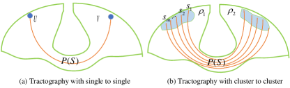
Figure 1: Tractography with different manners.

2 Methods

In its most basic form, a tractography algorithm takes two arbitrary points (voxels) of interest as input, labeled as a seed and a target, and yields the most likely trajectory on the given diffusion tensor vectorial field. Let $\Omega\subset{R^{3}}$ be the diffusion tensor vectorial field, and ${S_{U,V}}(t)\subset\Omega$ denotes a path that is parameterized by $t\in[0,T]$ connecting $U$ with $V$. Let $P(S)$ denote the probability of paths $S$ representing an anatomically genuine fiber trajectory in diffusion native space $\Omega\subset{R^{3}}$, which can be defined as,

$$P(s)=\int_{0}^{T}{p(s(t),\dot{s}(t))}{\rm{}}dt,$$ (1)

where $p\left({s(t),\dot{s}(t)}\right)$ is the metric representing the potential for the point $s(t)$ to be located inside a fiber bundle in the direction $\dot{s}(t)={{ds(t)}\mathord{\left/{\vphantom{{ds(t)}{dt}}}\right.\kern-1.2pt}{dt}}$. In an early deterministic tracking algorithm, (streamline tractography) [7, 39], $s(t)$ is computed to satisfy the Frenet equation [40],

$$\frac{{{\rm{d}}s(t)}}{{dt}}={V_{\max}}(s(t)),t\in\left[{0,T}\right],$$ (2)

where ${V_{\max}}(s(t))$ is the principal diffusion direction of $s(t)$. In a sense, this is a “greedy” algorithm, as it tries to find the optimal fiber trajectory. The inherent unreliability and inaccuracy of deterministic fiber tracking have driven the introduction of new tracking algorithms. Stochastic tractography algorithms [41, 42] probabilistically generate the tracing directions based on the fiber conditional probability density function and the probability of direction within each voxel is commonly defined as ODF at the center of a voxel. Filter tractography algorithms use their current model state to obtain the predicted signal and combine the measured signal to propagate forward in most consistent direction. While shortest path methods aim to find an optimal path by computing the maximum energy between two seeds. In this paper, we are interested in the particular case of computing the diffusion tensor field on a Riemannian manifold [42, 43], which is a potential under the form $p\left({s(.),\dot{s}(.)}\right)=\sqrt{\dot{s}{{(.)}^{T}}{\rm M}(s(.))\dot{s}(.)}$ describing an infinitesimal distance along the fiber path $S$ relative to the metric tensor $M$ (symmetric definite positive). In this situation, finding the curve connecting two points that globally minimizes the energy [44] is a shortened path called a geodetic [45, 46]. In [47], a variational model is proposed based on Hamilton-Jacobi-Bellman, in which an infinite number of particles start from a given seed region evolving along the streamline orientation given by the gradient of the defined cost function to reach the seed target. In our recent work [17, 34], penalized geodesic tractography based on a Finsler metric with a global optimization framework is introduced to improve cortical connectomics. These methods are related to an optimal control problem and turn out to be very useful for establishing the connectivity of a single point on the seed region but provide little information about the connectivity between two regions. [48] attempted to introduce optimal mass transportation to describe the connectivity between two cerebral regions. Unfortunately, it is only a preliminary mathematical description without algorithmic implementation and validation. Herein, we will focus here on the bundle structure tractography connecting two cerebral regions in a ‘cluster to cluster’ manner (Fig. 1b). Considering two given regions ${\rho_{1}}$ and ${\rho_{2}}$, the optimal fiber bundle can be viewed as a superposition of non-intertwined fiber streamline cluster $S(t)$ starting from ${\rho_{1}}$ to ${\rho_{2}}$ along the diffusion tensor vector field, and the energy $P(S)$ assigned to the streamline cluster is defined as,

$$P(S)=\int_{\rm{0}}^{T}{p\left({S(t),\dot{S}(t)}\right)}{\rm{}}dt,$$ (3)

where $S(0)={\rho_{1}}$, $S(T)={\rho_{2}}$ and $\dot{S}(t)$ is the diffusion vector field between ${\rho_{1}}$ and ${\rho_{2}}$. We first define the $S(t)$ and $\dot{S}(t)$, and $p\left({S(t),\dot{S}(t)}\right)$. In Section 2.1, we define the BTD function $S(t)$ on the diffusion vector field $\dot{S}(t)$ from ${\rho_{1}}$ to ${\rho_{2}}$ based on a higher-order streamline differential equation. For bundle continuity, we add spatial continuity constraint equation in Section 2.2. Then, the $S(t)$ solution can be simplified as estimation of BTD coefficients, detailed process is shown in Section 2.3.

2.1 Bundle-specific tractogram distribution function

Consider the diffusion field vector at position $(x,y,z)$ to be

$$v(x,y,z)={\left[{{v_{x}}(x,y,z),{v_{y}}(x,y,z),{v_{z}}(x,y,z)}\right]^{T}}.$$ (4)

The BTD can be parameterized by a 3D fiber bundle with a set of streamlines $S(t)=\left\{{{s_{i}},i=1,\cdots,\lambda}\right\}$ that satisfies the following properties [34]:

The tangent vector at point $(x,y,z)$ of fiber path ${s_{i}}$ equals the field vector $v(x,y,z)={\left[{{v_{x}}(x,y,z),{v_{y}}(x,y,z),{v_{z}}(x,y,z)}\right]^{T}}$, that is,

$$\frac{{\partial{s_{i}}}}{{\partial x}}{\rm{}}={\rm{}}{v_{x}}(x,{\rm{}}y,{\rm{}}z){\rm{}},{\rm{}}\frac{{\partial{s_{i}}}}{{\partial y}}{\rm{}}={\rm{}}{v_{y}}(x,{\rm{}}y,{\rm{}}z){\rm{}},{\rm{}}\frac{{\partial{s_{i}}}}{{\partial z}}={\rm{}}{v_{z}}(x,{\rm{}}y,{\rm{}}z){\rm{}}{\rm{.}}$$ (5)

The streamlines satisfy ${s_{i}}\cap{s_{j}}=0$, $i\neq j$, which is defined using the streamline differential equation,

$$\frac{{dx}}{{{v_{x}}(x,{\rm{}}y,{\rm{}}z)}}{\rm{}}={\rm{}}\frac{{dy}}{{{v_{y}}(x,{\rm{}}y,{\rm{}}z)}}=\frac{{dz}}{{{v_{z}}(x,{\rm{}}y,{\rm{}}z)}}.$$ (6)

We introduce the higher-order streamline differential Eq. 7 with the tangent vector approximated by the ${n^{th}}$-order polynomial,

$$f(x,y,z)=\sum\limits_{i=0}^{n}{\sum\limits_{j=0}^{n-i}{\sum\limits_{k=0}^{n-i-j}{a_{ijk}{x^{i}}{y^{j}}{z^{k}}}}},$$ (7)

where ${a_{ijk}}$ is the coefficients of the polynomial. Combined with Eq. 7, the diffusion vector $v(x,y,z)$ is denoted,

$$\begin{array}[]{l}v(x,y,z){\rm{=}}{\left[\begin{array}[]{l}\sum\limits_{i=0}^{n}{\sum\limits_{j=0}^{n-i}{\sum\limits_{k=0}^{n-i-j}{a_{ijk}^{x}{x^{i}}{y^{j}}{z^{k}}}}}\\ \sum\limits_{i=0}^{n}{\sum\limits_{j=0}^{n-i}{\sum\limits_{k=0}^{n-i-j}{a_{ijk}^{y}{x^{i}}{y^{j}}{z^{k}}}}}\\ \sum\limits_{i=0}^{n}{\sum\limits_{j=0}^{n-i}{\sum\limits_{k=0}^{n-i-j}{a_{ijk}^{z}{x^{i}}{y^{j}}{z^{k}}}}}\end{array}\right]^{T}}\\ {\rm{=}}A\cdot C(x,y,z){\rm{}}\end{array}$$ (8)

where $A$ is the coefficient matrix defined as,

$$A={\left[\begin{array}[]{l}a_{n00}^{x}{\rm{}}a_{(n-1)10}^{x}{\rm{}}a_{(n-1)01}^{x}{\rm{}}a_{(n-1)00}^{x}{\rm{}}...{\rm{}}a_{001}^{x}{\rm{}}a_{000}^{x}\\ a_{n00}^{y}{\rm{}}a_{(n-1)10}^{y}{\rm{}}a_{(n-1)01}^{y}{\rm{}}a_{(n-1)00}^{y}{\rm{}}...{\rm{}}a_{001}^{y}{\rm{}}a_{000}^{y}\\ a_{n00}^{z}{\rm{}}a_{(n-1)10}^{z}{\rm{}}a_{(n-1)01}^{z}{\rm{}}a_{(n-1)00}^{z}{\rm{}}...{\rm{}}a_{001}^{z}{\rm{}}a_{000}^{z}\end{array}\right]_{\left({3\sum\limits_{\Delta=0}^{n}{\frac{{(\Delta+1)*(\Delta+2)}}{2}}}\right)}}$$

and $C(x,y,z)$ denotes as,

$$\begin{array}[]{l}{C_{n}}(x,y,z)={({[{x^{n}},{x^{n-1}}y,{x^{n-1}}z,{x^{n-1}}{\rm{,}}\cdot\cdot\cdot,z{\rm{,}}1{\rm{}}]^{T}})_{\left({\sum\limits_{\Delta=0}^{n}{\frac{{(\Delta+1)*(\Delta+2)}}{2}}{\rm{,1}}}\right)}}\\ {\rm{=[}}{{\rm{F}}_{n}}(x,y,z){\rm{,}}{C_{n-1}}(x,y,z)]\\ \left\{\begin{array}[]{l}{C_{1}}(x,y,z)=[x,y,z,1],{\rm{}}\\ {F_{n}}(x,y,z)=[{c_{m}},{\rm{}}\cdot\cdot\cdot{\rm{}},{c_{l}},\cdot\cdot\cdot{\rm{}}{c_{2}}{\rm{,}}{c_{1}}],{\rm{}}m=(n+1)(n+2)/2\\ {c_{l}}={x^{i}}{y^{j}}{z^{k}}{\rm{with}}\\ {\rm{}}l=i(n-\frac{{i-3}}{2})+j+1,{\rm{}}i=[0,1,\cdot\cdot\cdot,n],{\rm{}}\\ j=[0,1,\cdot\cdot\cdot,n-i],{\rm{}}i+j+k=n\end{array}\right.\end{array}$$ (9)

To further illustrate the Eq. 9, we give an example of ${C_{n}}$ with $n=2$, The $n$ represented the order of higher-order streamline differential equation

$$\begin{array}[]{l}{C_{2}}(x,y,z){\rm{=[}}{{\rm{F}}_{2}}(x,y,z){\rm{,}}{C_{1}}(x,y,z)]\\ {\rm{}}=[{x^{2}},{y^{2}},{z^{2}},x{y},x{z},yz,x,y,z,{1}]\\ \left\{\begin{array}[]{l}{C_{1}}(x,y,z)=[x,y,z,1]{\rm{}}\\ {F_{2}}(x,y,z)=[{c_{6}},{c_{5}},{c_{4}},{c_{3}},{\rm{}}{c_{2}}{\rm{,}}{c_{1}}]{\rm{with}}\\ {\rm{}}{c_{6}}={x^{2}},{c_{5}}={y^{2}},{c_{4}}={z^{2}},{c_{3}}=x{y},{c_{12}}=x{z},{c_{1}}=y{z}\end{array}\right.\end{array}$$

2.2 Spatial continuity constraint equation for a tractogram

We assume that the diffusion displacement of water molecules in the same fiber maintains continuity. We use continuous incompressible fluid theory to describe the spatial continuity of the bundle by introducing the concept of divergence of the fiber flow on diffusion tensor vectorial field,

$$divS=\frac{{\partial{v_{x}}}}{{\partial x}}+\frac{{\partial{v_{y}}}}{{\partial y}}+\frac{{\partial{v_{z}}}}{{\partial z}}.$$ (10)

We assume that the fibers do not originate or terminate in the white matter, that is, $divS$ satisfies

$$divS=0.$$ (11)

The substitution of Eq. 8, and Eq. 10 into Eq. 11 yields:

$$\begin{array}[]{l}divS=\sum\limits_{i=0}^{n}{\sum\limits_{j=0}^{n-i}{\sum\limits_{k=0}^{n-i-j}{\left(\begin{array}[]{l}a_{ijk}^{x}i{x^{i-1}}{y^{j}}{z^{k}}+\\ a_{ijk}^{y}j{x^{i}}{y^{j-1}}{z^{k}}+\\ a_{ijk}^{z}k{x^{i}}{y^{j}}{z^{k-1}}\end{array}\right){\rm{}}}}}\\ {\rm{=}}{H_{n-1}}\cdot{C_{n-1}}(x,y,z)=0\end{array}$$ (12)

where ${C_{n-1}}(x,y,z)$ can be derived from Eq. 9, and

$${C_{n-1}}(x,y,z)={[{x^{n-1}},{x^{n-2}}y,{x^{n-2}}z,\cdot\cdot\cdot,{x^{i}}{y^{j}}{z^{k}},\cdot\cdot\cdot,z,1]_{\left(M,1\right)}}$$

$${H_{n-1}}={\left[\begin{array}[]{l}na_{n00}^{x}{\rm{+}}a_{(n-1){\rm{1}}0}^{y}{\rm{+}}a_{(n-1)01}^{z}{\rm{}}\\ (n-1)a_{(n-1)10}^{x}{\rm{+2}}a_{{\rm{(n-2)2}}0}^{y}{\rm{+}}a_{(n-2)11}^{z}\\ (n-1)a_{(n-1)01}^{x}{\rm{+}}a_{(n-2)11}^{y}{\rm{+2}}a_{(n-2)02}^{z}\\ (n-1)a_{(n-1)00}^{x}{\rm{+}}a_{(n-2)10}^{y}{\rm{+}}a_{(n-2)01}^{z}\\ \cdot\cdot\cdot\\ {\rm{(}}i{\rm{+1)}}a_{(i+1)jk}^{x}+(j+1)a_{i(j+1)k}^{y}+\\ (k+1)a_{ij(k+1)}^{z}\\ \cdot\cdot\cdot\\ a_{101}^{x}{\rm{+}}a_{011}^{y}{\rm{+2}}a_{002}^{z}\\ a_{100}^{x}{\rm{+}}a_{010}^{y}{\rm{+}}a_{001}^{z}\end{array}\right]^{T}}_{\left(1,M\right)}$$

where $M=\sum\limits_{\Delta=0}^{n}{\frac{{(\Delta)*(\Delta+1)}}{2}}$.

2.3 Estimation of the BTD

With the definition of BTD, finding the optimal tractogram from ${\rho_{1}}$ to ${\rho_{2}}$ can be simplified as the estimation of coefficient matrix $A$. The coefficient matrix $A$ is estimated by minimizing the energy $P(S)$ in Eq. 4 with $p\left({S(t),\dot{S}(t)}\right)$ defined as:

$$p\left({S(t),\dot{S}(t)}\right)=\left\|{\Phi(v(x,y,z))-v(x,y,z)}\right\|_{2}^{2}$$ (13)

where $\Phi(v(x,y,z))$ is the probability that fiber trajectory is actually passes through the FOD at point $(x,y,z)$, which is derived from the orientation distribution functions (ODF) in each voxel in the volume. To achieve fiber spatial continuity, we add constrain Eq. 12 to Eq. 4, which yields the optimization model:

$$\begin{array}[]{l}\mathop{\min}\limits_{S}P(S)=\iiint_{\Omega}{\left\|{\Phi(v(x,y,z))-v(x,y,z)}\right\|_{2}^{2}dxdydz}\\ s.t.{\rm{}}{H_{n-1}}\cdot{C_{n-1}}(x,y,z)=0\end{array}$$ (14)

where $\Omega=[{\omega_{1}},{\omega_{2}},\cdot\cdot\cdot,{\omega_{\gamma}}]$ is the bundle pathway containing $\gamma$ voxels from ${\rho_{1}}$ to ${\rho_{2}}$. For simplicity, we approximate $\Phi(v(x,y,z))$ as the peak direction values in each voxel and set $[G={[{g_{1}}{\rm{,}}{g_{2}}\cdot\cdot\cdot{g_{\gamma}}]_{\left({3,{\rm{}}\gamma}\right)}}$ as a set of peak direction values in $\omega$. The $(X,Y,Z)$ is the center of a voxel in $\omega$ and $C_{n}^{*}(X,Y,Z)$ is a set of $C_{n}(X,Y,Z)$. The estimation of coefficient matrix $A$ of BTD is simplified as

$$\mathop{\min}\limits_{A}E=\left\|{G-A\cdot C_{n}^{*}(X,Y,Z)}\right\|_{2}^{2}$$

$$s.t.{\rm{}}{H_{n-1}}\cdot C_{n-1}^{*}(X,Y,Z)=0$$

$$\begin{array}[]{l}\begin{split}C_{n}^{*}(X,Y,Z)=&[C_{n}({X_{1}},{Y_{1}},{Z_{1}}),C_{n}({X_{2}},{Y_{2}},{Z_{2}}),\\ &\cdot\cdot\cdot,C_{n}({X_{\gamma}},{Y_{\gamma}},{Z_{\gamma}})]_{\left({\sum\limits_{\Delta=0}^{n}{\frac{{(\Delta+1)*(\Delta+2)}}{2}},{\rm{}}\gamma}\right)}\end{split}\end{array}$$ (15)

The estimation of the BTD is decomposed into two stages. First, the least squares method is used to solve Eq. 15 to obtain the coefficient matrix $A$. Second, we use the coefficient matrix $A$ to obtain the flow field vectors and use the fourth-order Runge-Kutta method [28] to solve the higher-order streamline differential equation Eq. 6. See Algorithm. 1 for a detailed implementation.

Input: A set of peak directions $G={[{g_{1}}{\rm{,}}{g_{2}}\cdot\cdot\cdot{g_{\gamma}}]_{\left({3,{\rm{}}\gamma}\right)}}$ , the center coordinate $(X,Y,Z)$ of each voxel in bundle mask $\Omega$, seed points $\left\{{{\beta_{i}},i=1,\cdots,\lambda}\right\}$, tractography step size $\Delta$.

Output: Tractogram $S$.

Calculate $C_{n}^{*}(X,Y,Z)$ and $C_{n-1}^{*}(X,Y,Z)$ using $(X,Y,Z)$ in $\Omega$ with Eq. 9.

Calculate $H_{n-1}$ according to $C_{n-1}^{*}(X,Y,Z)$ by Eq. 12.

Estimate coefficients matrix $A$ with Eq. 15.

Calculate tractogram $S=\left\{{{s_{i}},i=1,\cdots,\lambda}\right\}$ in $\Omega$.

Take seed ${\beta_{i}}$ as starting points of the tractogram $S$.

for $i=1\to\lambda$ do

       set $\eta(0)$ as starting point of $S_{i}$

       $\eta(0)={\beta_{i}}$, $t=0$

       while $\eta(t)\in\Omega$ do

             Calculate flow field direction at point $\eta(t)$

             $v(\eta(t))=A\cdot{C_{n}}(\eta(t))$

             Calculate the next point of $S_{i}$ with Eq. 6

             $\eta(t+1)=RungeKutta({\rm{}}\eta(t),v(\eta(t)),\Delta)$

             ${s_{i}}=[\eta(0),\cdots,{\rm{}}\eta(t)]$

             $t=t+1$

            

      $S=\left\{{{s_{i}},i=1,\cdots,\lambda}\right\}$

Algorithm 1 Estimation of the bundle-specific tractogram distribution function.

3 Experiments

Tests and validations of our algorithm are based on four simulated datasets, namely, Hough data, Sine data [28], Circle data, and ISMRM 2015 Tractography Challenge data [1], and in vivo data of HCP [49]. Our BTD estimation is based on FODs estimated using constrained spherical deconvolution, which are included in the software package MRtrix [11]. The experimental results are evaluated by comparing BTD with deterministic FOD-based tracking (SD_Stream) [50], integration over fiber orientation distributions (iFOD2) [51], and unscented Kalman filter (UKF) algorithm [52]. For quantitative evaluation, we use Tractometer metrics, that is, valid connections (VC), bundle overlap (OL), and bundle overreach (OR) for Sine and Hough data [1, 53, 54]. For Circle data, we design a metric referred to as $Deviation$, which can be expressed as:

$$Deviation=\sum\limits_{j=1}^{N}{\sum\limits_{i=1}^{{\lambda_{j}}}{(\sqrt{{{({x_{ij}}-{U_{c}})}^{2}}+{{({y_{ij}}-{V_{c}})}^{2}}}}}-{R_{j}})/\sum\limits_{j=1}^{N}{({\lambda_{j}})}$$

where $N$ is the number of streamlines belonging to a bundle, and the $j$-th streamline has ${\lambda_{j}}$ points. The $({x_{ij}},{y_{ij}})$ is the $i$-th point on $j$-th streamline, and ${R_{j}}$ is the distance from a seed to circle center $(U_{c},V_{c})$ on $j$-th streamline. In addition, we compute the bundle volumetric overlap to quantify the spatial coverage [1].

3.1 Hough, Sine, Circle, and FiberCup data

We simulate three datasets: the Hough data feature brain-like large fanning connections, while the Sine data feature long-range and large twisting connections, and the Circle data feature large bending connections. The datasets are generated with the following parameter settings. The spatial resolution is $1mm\times 1mm\times 1mm$. There are 78 gradient directions with a b-value of 1000 $s/m{m^{2}}$, and the signal-to-noise ratio (SNR) is set to 10, 20, and $+\infty$. The Hough and Circle data size is $60\times 60\times 6$, and the Sine data size is $100\times 100\times 6$. Sine data satisfy ${\rm{2}}\pi\cdot{\rm{y}}=\alpha\cdot\sin(x)$, and $\alpha$ is set to 0.1, 0.2, 0.3, and 0.4 to adjust different amplitudes. The inner radius ($r_{1}$) of the circle data is 10 $mm$, and the outer radius ($r_{2}$) is 20 $mm$. FiberCup data were released in the MICCAI Challenge in 2009. The spatial resolution is $3mm\times 3mm\times 3mm$; the data have 30 gradient directions, with a b-value of 1000 $s/m{m^{2}}$ and a size of $64\times 64\times 3$.

Table 1: Comparison of Tractometer metrics of BTD using Hough data and Sine data with SD_Stream, and IFOD2.

	Hough			Sine		Sine
	(SNR=10)			(SNR=10, $\alpha=0.3$)		(SNR=10, $\alpha=0.4$)
	OL	VC	Time($s$)	OL	VC	OL	VC
3rd-order	0.6	0.67	2	0.65	0.19	0.54	0.25
4th-order	0.71	0.84	2.4	0.62	0.48	0.56	0.33
5th-order	0.79	0.93	5.8	0.64	0.57	0.57	0.39
6th-order	0.85	0.96	9.2	0.66	0.67	0.62	0.82
SD_Stream	0.65	0.80		0.45	0.16	0.39	0.04
iFOD2	0.82	0.95		0.62	0.55	0.51	0.05

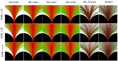
Figure 2: Comparison of tractography results of BTD with iFOD2 and SD_Stream at different SNRs using the Hough data.

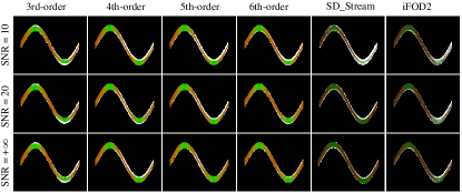
Figure 3: Comparison of tractography results of BTD with iFOD2 and SD_Stream at different SNRs using the Sine data ($\alpha=0.3$).

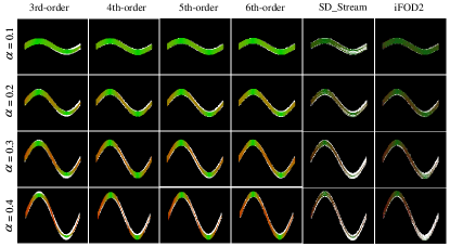
Figure 4: Comparison of tractography results of BTD with iFOD2 and SD_Stream at different $\alpha$ using Sine data (SNR=10).

Table 2: Comparison of Tractometer metrics of BTD using Circle data with SD_Stream, and IFOD2.

	SNR	5th-order	SD_Stream	iFOD2
VC	10	0.47	0.21	0.30
	20	0.60	0.28	0.40
	$+\infty$	0.61	0.39	0.58
OL	10	0.81	0.58	0.75
	20	0.83	0.64	0.79
	$+\infty$	0.90	0.62	0.85
Deviation (voxel)	10	0.48	0.88	1.61
	20	0.42	1.31	1.71
	$+\infty$	0.23	0.91	1.48

Tractography parameters are as follows. The step size $\lambda$ is 0.2$mm$. The seed region for the Hough data is the first six rows of voxels (bottom of the data), the Sine data is the first two columns of voxels (left side of the data), and the Circle data is the four rows of voxels in the red box (Fig. 5). The seed masks are the first four columns or rows in regions A1, B1, C1, D1 and E1 for FiberCup data. The number of seeds is set to 2000 for the Sine and Hough data and 720 for the Circle data, and there are 4 seeds in each voxel for the FiberCup data. The minimum length of any track is set to 5$mm$ (5 voxels) for the Hough and Sine data, 15$mm$ (5 voxels) for the FiberCup data, and ${\rm{2}}\pi\cdot{{\rm{r}}_{1}}$ mm for the Circle data.

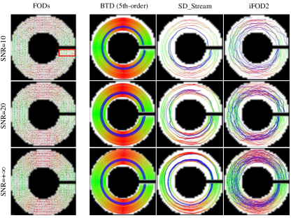
Figure 5: Comparison of tractography results of the BTD (5th-order) with iFOD2 and SD_Stream at SNRs of 10, 20, and $+\infty$ using Circle data. The blue color fibers (from the same starting area) are used to visualize the tractography deviation with different methods.

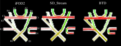
Figure 6: Comparison of tractography results of the BTD (5th-order) with iFOD2 and SD_Stream using FiberCup data.

To evaluate the tractograms of BTD on different orders, we test BTD from the 3rd- to 6th-order on Hough data and Sine ($\alpha=0.3$) data with SNRs of 10, 20, and $+\infty$, which are shown in Fig. 2 and Fig. 3. We further test the algorithms on Sine data with $\alpha$ from 0.1, 0.2, 0.3, and 0.4 (Fig. 4) to adjust the amplitude. The quantitative results of Hough data with SNR=10, Sine data with $\alpha=0.3$ and SNR=10, and Sine data with $\alpha=0.4$ and SNR=10 are shown in Table. 1. From Fig. 2, Fig. 3 and Table. 1 show the fitting ability increase, and the BTD with 5th-order and 6th-order yield better results than the 3th-order and 4th-order BTD. Compared to the 5th-order BTD, the 6th-order BTD shows approximate fitting ability but the complexity will increase significantly because the coefficients of the BTD from the 5th-order to the 6th-order will increase by 84 terms. Therefore, the 5th-order BTD is used to compare the tractography results in the following experiments. Notion, we can select the lower order of BTD when we track the simple bundles, which can reduce running time. However, for the complex bundle, like the corpus callosum, we suggested the higher order of BTD as the bundle is complex. Moreover, for most of the bundle in vivo, the fitting ability of 5th-order is sufficient and the run time is suitable. Therefore, we recommended the 5th-order of BTD for some complex bundles.

To further verify the proposed algorithm, we assess the tractograms using Circle data with SNRs of 10, 20, and $+\infty$, in which error accumulation is more obvious. The results are shown in Fig. 5 and Table. 2. The blue curves represent the fibers in the same starting area but with different trajectories. The ending points of the SD_Stream and iFOD2 deviate largely compared to their starting points.

To illustrate the model performance in one phantom image covering various streamline scenarios, we test BTD on FiberCup data. This data included crossing, fanning etc., which was widely used for comparison of tracking algorithms. The BTD has better performance for the bundles with crossing and twisting regions in Fig. 6. Furthermore, the BTD shows better VC, OL and OR in Table. 3.

Table 3: Comparison of Tractometer metrics of BTD using FiberCup data with SD_Stream, and IFOD2.

	Bundle	BTD	iFOD2	SD_Stream
VC	A1 A2	0.73	0.69	0.30
	B1 B2	0.54	0.48	0.32
	C1 C2	0.74	0.44	0.50
	D1 D2	0.73	0.64	0.33
	E1 E2	0.78	0.08	0.06
	E1 E3	0.46	0.10	0.15
	E1 E4	0.85	0.53	0.23
OL	A1 A2	0.50	0.47	0.43
	B1 B2	0.48	0.45	0.43
	C1 C2	0.62	0.43	0.41
	D1 D2	0.46	0.32	0.39
	E1 E2	0.42	0.14	0.13
	E1 E3	0.35	0.19	0.30
	E1 E4	0.45	0.35	0.17
OR	A1 A2	0.05	0.12	0.06
	B1 B2	0	0.02	0
	C1 C2	0.11	0.16	0.13
	D1 D2	0	0	0
	E1 E2, E3 E4	0	0.06	0.008

We compare the tractograms among 5th-order BTD, SD_Stream, and iFOD2. From Fig. 2, the tractograms of BTD are evenly distributed in the mask and have larger VC and OL than SD_Stream and iFOD2 with different SNRs. In addition, the tractograms of SD_Stream and iFOD2 show the small angle of divergence, and fewer fibers reach the large fanning regions on Hough data. As an important factor affecting tractography, error accumulation leads to premature termination of the fibers, which is more obvious in long-range and large twisting connections, such as the bundle on Sine data (Fig. 3). The BTD obtains larger spatial coverage as well as better VC and OL at different SNRs. To further compare the tractograms on more complex data, we adjust the from 0.1, 0.2, 0.3, and 0.4 for Sine data (Fig. 4). The BTD shows more stable tractograms and higher VC and OL, while SD_Stream and iFOD2 exhibit an increase in the number of prematurely terminated fibers with decreasing amplitude. In Fig. 5, the BTD shows less deviation with increasing noise and most of fibers can return their starting points. In Fig. 6 and Table. 3, the BTD shows better performance compared with SD_Stream and iFOD2, specifically for the bundles with crossing and fanning (E1-E2, E1-E4). The BTD shows large VC and OL and lower OR compared with SD_Stream and iFOD2. Additionally, the computational time from 3th- to 6th-order BTD may be need approximately 2.0s, 2.4s, 5.8s and 9.2s runtime using Hough data (repeat 100 times; in fourth column in Table. 1) with Inter i-9900k processor and Matlab2019 platform.

From the above results, the BTD has more valid fibers, larger spatial coverage, and lower error accumulation as fibers spread forward than SD_Stream and iFOD2. The BTD seems to capture the better fanning, long-range and twisting, and large bending bundle tracking results.

3.2 ISMRM 2015 Tractography Challenge data

In this section, we evaluate the performance of the BTD on the ISMRM 2015 Challenge data, which simulates the shape and complexity of 25 well-known in vivo fiber bundles. The dataset has 32 gradient directions, a b-value of 1000 $s/m{m^{2}}$, and 2$mm$ isotropic voxels. The dataset is denoised and corrected for distortions using MRtrix3 ($dwidenoise$ and $dwipreproc$). The tractography parameters are as follows: The min-separation angle is $30_{0}$, the step size is 0.2$mm$, and the minimum length of any track is more than 50 $mm$. FODs are performed by standard constrained spherical deconvolution (CSD) in MRtrix for iFOD2 and SD_Stream, and the UKF uses a two-tensor model.

Table 4: Comparison of Tractometer metrics of BTD using ISMRM 2015 tractography challenge data with UKF, SD_Stream, and IFOD2.

	CST-L			CST-R
	VC	OL	OR	VC	OL	OR
BTD	0.79	0.80	0.09	0.72	0.85	0.10
UKF	0.26	0.77	0.23	0.19	0.84	0.21
iFOD2	0.23	0.74	0.18	0.34	0.72	0.19
SD_Stream	0.10	0.57	0.11	0.16	0.53	0.13

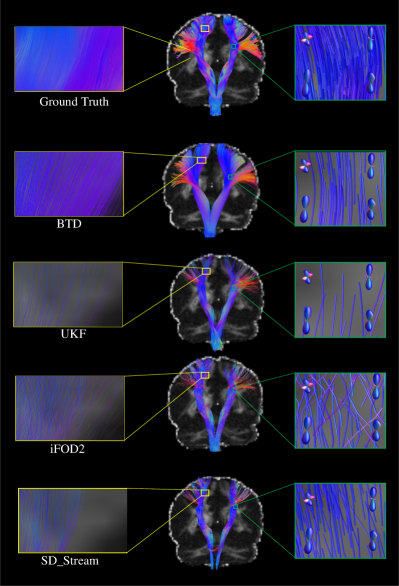
Figure 7: Comparison of tractography results of BTD with UKF, iFOD2, and SD_Stream on CST using ISMRM 2015 Tractography Challenge data.

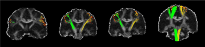
Figure 8: Slices and fibers of BTD on ISMRM 2015 Tractography Challenge data.

We selected the corticospinal tract (CST) as an example to test the algorithms. The CST has the features of large fanning and long range. The anatomy of CST is well known from the brainstem to the precentral gyrus [55]. The bundle masks are the voxels that ground truth fibers pass through after dilatation. In Fig. 7, we exhibit the details of the CST near area 4t (yellow boxes) and another regions (green boxes)(Brainetome regions [56]). Tractometer metrics with VC, OR, and OL for left and right CST are presented in Table. 4.

From the right column in Fig. 7, the BTD preserves better spatial fluency and is closer to the ground truth. The BTD tractography more fibers ending in precentral gyrus than iFOD2, SD_Stream, and UKF methods. While the UKF shows some twisted fibers and is unevenly distributed. The iFOD2 and SD_Stream show sparse and interrupted fibers. The BTD can track the large fanning fibers that ending nearby 4tl and 4hf in precentral gyrus. The iFOD2 and SD_Stream show fewer or no fibers in these regions. We can see that the VC and OL of iFOD2 and SD_Stream in Table. 4 are lower than BTD and UKF. In addition, the BTD has a lower OR compared with other three algorithms. The BTD seems to capture the complexity in regions where we expect fiber geometry (details are shown in Fig. 8). This is because the BTD reconstructs a bundle in a ‘cluster to cluster’ manner to reduce the ambiguous spatial correspondences between diffusion directions and fiber geometry. Therefore, the BTD preserves better spatial fluency and can better track the complex fibers than current peak-based tractography.

3.3 HCP data

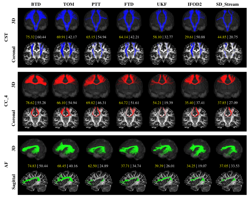
Figure 9: Qualitative comparison of tractography results reconstruction of CST, CC_4, and AF on HCP #100307 subject. Top: the 3D display of tracked fiber bundles. Bottom: the slice display of tracked fiber bundles on the FA images. Middle: the quantitative comparison of different tractography methods with tractometer metrics (VC(%) $|$ OL(%)).

For visual and quantitative comparisons on data from real subjects, we used the HCP dataset subjects [49]. These are acquired using 288 gradient directions, consisting of 18 scans at b = 0 $s/m{m^{2}}$ and three b-values (1000 $s/m{m^{2}}$, 2000 $s/m{m^{2}}$, 3000 $s/m{m^{2}}$) using 90 gradients, and the voxel size is 1.25$mm$ × 1.25$mm$ × 1.25$mm$. We used the preprocessed dMRI images shared by HCP. FODs were estimated using constrained spherical deconvolution, which are included in the software package MRtrix [11].

We used HCP #100307 subject to visually compare fiber tractograms from the proposed BTD algorithm and results from the tract orientation mapping (TOM) [57], parallel transport tractography (PTT) [33], fiber trajectory distribution (FTD) [34], unscented Kalman filter (UKF) algorithm [52], integration over fiber orientation distributions (iFOD2) [51], and deterministic FOD-based tracking (SD_Stream) [50]. In this paper, we use VC and OL to validate the proposed method, so all tractography methods were selected 3000 streamlines which were seeded from all voxels within the each tract start regions, and tract masks were used to filter the tractograms. The tractography specific parameters are as follows: i) FTD, iFOD2, and SD_Stream: maximum angle = $60^{0}$, step size = 0.3, cutoff = 0.1, minimum length = 75; ii) UKF: seedingFA = 0.06, stoppingFA = 0.05, stoppingThreshold = 0.06, Qm = 0.001, and Ql = 50. iii) PTT: the default parameters in [33], the difference is that the seeding regions are the tract start regions. iv) TOM: the default parameters in [57], the difference is that the seeding regions are the tract start regions, max_nr_fibers=3000, no streamline filtering by end mask.

In the absence of ground truth fibers for in vivo data, the relatively familiar corpus callosum (CC_4), CST, and arcuate fasciculus (AF) were selected for qualitative and quantitative evaluations. The AF is a neuronal pathway that connects Wernicke’s area and Broca’s area [58]. The CC_4 is minor forceps of the corpus callosum that connects bilateral frontal lobe [59]. These three tracts have the characteristics of long-range, twisting, and fanning characteristics, making them suitable to assess the algorithms.

The main lost fibers in the TOM, PTT, FTD, UKF, iFOD2, and SD_Stream are mainly distributed in fanning and other complex geometric structures, such as the fibers ending in area 4tl and 4hf of precentral gyrus (CST), frontal lobe on CC_4 and temporal lobes on AF. The results are consistent with VC and OL in middle of Fig. 9, in which the BTD obtains highest VC and OL. We also exhibited the fibers of AF and CC_4 on anatomical slices in top of Fig. 9 (the slices and fibers of CC_4 can be seen in bottom of Fig. 9). In addition, the BTD of 7th-order or higher may overfit in the termination region.

In addition, we also give tractometer metrics results of the proposed BTD on CST using five HCP data (subject ID: #100307, #112112, #112920, #113821, #118831) in Fig. 10. The results show that the proposed method is higher than the other compared methods in VC and OL tractometer metrics. We can also see that BTD has a significant improvement compared to FTD, which illustrates the advantage of BTD for complex bundle reconstruction by establishing higher-order streamline differential equations at the global level.

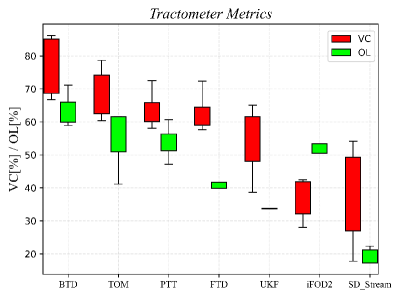
Figure 10: Box-plots of tractometer metrics comparing reconstruction of CST using the proposed BTD with other tractography methods.

4 Discussion and Conclusion

In this work, a novel bundle-specific tractography approach BTD is proposed, which integrates higher-order streamline differential equation to derive brain connectome between two regions in ‘cluster to cluster’ manner instead of ‘single to single’ manner. We parameterize fiber bundles using the BTD coefficients that are estimated by minimizing the energy on the diffusion tensor vector field by combining the priors. Experiments are performed on Hough, Sine, Circle data, and the ISMRM 2015 Tractography Challenge data and in vivo data of HCP for qualitative and quantitative evaluation. The horizontal comparisons show that with increasing order of the BTD, the numbers of valid fibers and overlapped regions will gradually increase. The best results are obtained with the 5th- or 6th-order BTD, and an order higher than six may cause overfitting. The comparisons with state-of-the-art methods show that the BTD can reconstruct complex fiber bundles, such as long-range, large twisting, and fanning tracts, and show better spatial consistency with fiber geometry, which is potentially useful for robust tractography.

Our method may be affected when FODs or peaks are inaccurate due to noise, artifacts, pathological cases, or poor-quality datasets. In addition, the BTD has difficulty tracking bundles that have received tumor compression. Fiber tracking using deep learning in tumor scenarios will be studied in future work.

References

- [1] K. H. Maier-Hein, P. F. Neher, J.-C. Houde, M.-A. Côté, E. Garyfallidis, J. Zhong, M. Chamberland, F.-C. Yeh, Y.-C. Lin, Q. Ji et al., “The challenge of mapping the human connectome based on diffusion tractography,” Nature Communications, vol. 8, no. 1, p. 1349, 2017.
- [2] S. Mori and P. C. Van Zijl, “Fiber tracking: principles and strategies–a technical review,” NMR in Biomedicine: An International Journal Devoted to the Development and Application of Magnetic Resonance In Vivo, vol. 15, no. 7-8, pp. 468–480, 2002.
- [3] S. Jbabdi and H. Johansen-Berg, “Tractography: where do we go from here?” Brain Connectivity, vol. 1, no. 3, pp. 169–183, 2011.
- [4] L. Xie, J. Huang, J. Yu, Q. Zeng, Q. Hu, Z. Chen, G. Xie, and Y. Feng, “Cntseg: A multimodal deep-learning-based network for cranial nerves tract segmentation,” Medical Image Analysis, vol. 86, p. 102766, 2023.
- [5] M. Descoteaux, R. Deriche, T. R. Knosche, and A. Anwander, “Deterministic and probabilistic tractography based on complex fibre orientation distributions,” IEEE Transactions on Medical Imaging, vol. 28, no. 2, pp. 269–286, 2008.
- [6] S. Jbabdi, S. N. Sotiropoulos, S. N. Haber, D. C. Van Essen, and T. E. Behrens, “Measuring macroscopic brain connections in vivo,” Nature Neuroscience, vol. 18, no. 11, pp. 1546–1555, 2015.
- [7] B. Jeurissen, A. Leemans, D. K. Jones, J.-D. Tournier, and J. Sijbers, “Probabilistic fiber tracking using the residual bootstrap with constrained spherical deconvolution,” Human Brain Mapping, vol. 32, no. 3, pp. 461–479, 2011.
- [8] P. Poulin, D. Jörgens, P.-M. Jodoin, and M. Descoteaux, “Tractography and machine learning: Current state and open challenges,” Magnetic Resonance Imaging, vol. 64, pp. 37–48, 2019.
- [9] F. Rheault, P. Poulin, A. V. Caron, E. St-Onge, and M. Descoteaux, “Common misconceptions, hidden biases and modern challenges of dmri tractography,” Journal of Neural Engineering, vol. 17, no. 1, p. 011001, 2020.
- [10] C.-H. Yeh, D. K. Jones, X. Liang, M. Descoteaux, and A. Connelly, “Mapping structural connectivity using diffusion mri: challenges and opportunities,” Journal of Magnetic Resonance Imaging, vol. 53, no. 6, pp. 1666–1682, 2021.
- [11] J.-D. Tournier, F. Calamante, and A. Connelly, “Mrtrix: diffusion tractography in crossing fiber regions,” International Journal of Imaging Systems and Technology, vol. 22, no. 1, pp. 53–66, 2012.
- [12] M. Ankele, L.-H. Lim, S. Groeschel, and T. Schultz, “Versatile, robust, and efficient tractography with constrained higher-order tensor fodfs,” International Journal of Computer Assisted Radiology and Surgery, vol. 12, pp. 1257–1270, 2017.
- [13] S. Cetin, E. Ozarslan, and G. Unal, “Elucidating intravoxel geometry in diffusion-mri: asymmetric orientation distribution functions (aodfs) revealed by a cone model,” in Medical Image Computing and Computer-Assisted Intervention–MICCAI 2015: 18th International Conference, Munich, Germany, October 5-9, 2015, Proceedings, Part I 18. Springer, 2015, pp. 231–238.
- [14] S. N. Sotiropoulos, T. E. Behrens, and S. Jbabdi, “Ball and rackets: inferring fiber fanning from diffusion-weighted mri,” NeuroImage, vol. 60, no. 2, pp. 1412–1425, 2012.
- [15] M. Reisert, E. Kellner, and V. G. Kiselev, “About the geometry of asymmetric fiber orientation distributions,” IEEE Transactions on Medical Imaging, vol. 31, no. 6, pp. 1240–1249, 2012.
- [16] M. Bastiani, M. Cottaar, K. Dikranian, A. Ghosh, H. Zhang, D. C. Alexander, T. E. Behrens, S. Jbabdi, and S. N. Sotiropoulos, “Improved tractography using asymmetric fibre orientation distributions,” NeuroImage, vol. 158, pp. 205–218, 2017.
- [17] Y. Wu, Y. Hong, Y. Feng, D. Shen, and P.-T. Yap, “Mitigating gyral bias in cortical tractography via asymmetric fiber orientation distributions,” Medical Image Analysis, vol. 59, p. 101543, 2020.
- [18] H.-H. Ehricke, K.-M. Otto, and U. Klose, “Regularization of bending and crossing white matter fibers in mri q-ball fields,” Magnetic Resonance Imaging, vol. 29, no. 7, pp. 916–926, 2011.
- [19] T. E. Behrens, H. J. Berg, S. Jbabdi, M. F. Rushworth, and M. W. Woolrich, “Probabilistic diffusion tractography with multiple fibre orientations: What can we gain?” NeuroImage, vol. 34, no. 1, pp. 144–155, 2007.
- [20] C. Ye and J. L. Prince, “Probabilistic tractography using lasso bootstrap,” Medical Image Analysis, vol. 35, pp. 544–553, 2017.
- [21] J. Pontabry, F. Rousseau, E. Oubel, C. Studholme, M. Koob, and J.-L. Dietemann, “Probabilistic tractography using q-ball imaging and particle filtering: application to adult and in-utero fetal brain studies,” Medical Image Analysis, vol. 17, no. 3, pp. 297–310, 2013.
- [22] S. Khalsa, S. D. Mayhew, M. Chechlacz, M. Bagary, and A. P. Bagshaw, “The structural and functional connectivity of the posterior cingulate cortex: Comparison between deterministic and probabilistic tractography for the investigation of structure–function relationships,” NeuroImage, vol. 102, pp. 118–127, 2014.
- [23] V. Wegmayr and J. M. Buhmann, “Entrack: Probabilistic spherical regression with entropy regularization for fiber tractography,” International Journal of Computer Vision, vol. 129, pp. 656–680, 2021.
- [24] J. G. Malcolm, M. E. Shenton, and Y. Rathi, “Filtered multitensor tractography,” IEEE Transactions on Medical Imaging, vol. 29, no. 9, pp. 1664–1675, 2010.
- [25] R. Liao, L. Ning, Z. Chen, L. Rigolo, S. Gong, O. Pasternak, A. J. Golby, Y. Rathi, and L. J. O’Donnell, “Performance of unscented kalman filter tractography in edema: Analysis of the two-tensor model,” NeuroImage: Clinical, vol. 15, pp. 819–831, 2017.
- [26] S. Jbabdi, M. W. Woolrich, J. L. Andersson, and T. Behrens, “A bayesian framework for global tractography,” NeuroImage, vol. 37, no. 1, pp. 116–129, 2007.
- [27] A. Lemkaddem, D. Skiöldebrand, A. Dal Palú, J.-P. Thiran, and A. Daducci, “Global tractography with embedded anatomical priors for quantitative connectivity analysis,” Frontiers in Neurology, vol. 5, p. 232, 2014.
- [28] I. Aganj, C. Lenglet, N. Jahanshad, E. Yacoub, N. Harel, P. M. Thompson, and G. Sapiro, “A hough transform global probabilistic approach to multiple-subject diffusion mri tractography,” Medical Image Analysis, vol. 15, no. 4, pp. 414–425, 2011.
- [29] P. Fillard, C. Poupon, and J.-F. Mangin, “A novel global tractography algorithm based on an adaptive spin glass model.” in MICCAI (1), 2009, pp. 927–934.
- [30] J.-F. Mangin, P. Fillard, Y. Cointepas, D. Le Bihan, V. Frouin, and C. Poupon, “Toward global tractography,” NeuroImage, vol. 80, pp. 290–296, 2013.
- [31] I. Nelkenbaum, G. Tsarfaty, N. Kiryati, E. Konen, and A. Mayer, “Automatic segmentation of white matter tracts using multiple brain mri sequences,” in 2020 IEEE 17th International Symposium on Biomedical Imaging (ISBI). IEEE, 2020, pp. 368–371.
- [32] M. Cottaar, M. Bastiani, N. Boddu, M. F. Glasser, S. Haber, D. C. Van Essen, S. N. Sotiropoulos, and S. Jbabdi, “Modelling white matter in gyral blades as a continuous vector field,” NeuroImage, vol. 227, p. 117693, 2021.
- [33] D. B. Aydogan and Y. Shi, “Parallel transport tractography,” IEEE Transactions on Medical Imaging, vol. 40, no. 2, pp. 635–647, 2020.
- [34] Y. Feng and J. He, “Asymmetric fiber trajectory distribution estimation using streamline differential equation,” Medical Image Analysis, vol. 63, p. 101686, 2020.
- [35] R. E. Smith, J.-D. Tournier, F. Calamante, and A. Connelly, “Anatomically-constrained tractography: improved diffusion mri streamlines tractography through effective use of anatomical information,” NeuroImage, vol. 62, no. 3, pp. 1924–1938, 2012.
- [36] F. Rheault, E. St-Onge, J. Sidhu, K. Maier-Hein, N. Tzourio-Mazoyer, L. Petit, and M. Descoteaux, “Bundle-specific tractography with incorporated anatomical and orientational priors,” NeuroImage, vol. 186, pp. 382–398, 2019.
- [37] M. F. Glasser, S. M. Smith, D. S. Marcus, J. L. Andersson, E. J. Auerbach, T. E. Behrens, T. S. Coalson, M. P. Harms, M. Jenkinson, S. Moeller et al., “The human connectome project’s neuroimaging approach,” Nature Neuroscience, vol. 19, no. 9, pp. 1175–1187, 2016.
- [38] D. C. Van Essen, S. M. Smith, D. M. Barch, T. E. Behrens, E. Yacoub, K. Ugurbil, W.-M. H. Consortium et al., “The wu-minn human connectome project: an overview,” NeuroImage, vol. 80, pp. 62–79, 2013.
- [39] B. Hu, B. Ye, Y. Yang, K. Zhu, Z. Kang, S. Kuang, L. Luo, and H. Shan, “Quantitative diffusion tensor deterministic and probabilistic fiber tractography in relapsing–remitting multiple sclerosis,” European Journal of Radiology, vol. 79, no. 1, pp. 101–107, 2011.
- [40] P. J. Basser, “Fiber-tractography via diffusion tensor mri (dt-mri),” in Proceedings of the 6th Annual Meeting ISMRM, Sydney, Australia, vol. 1226, 1998.
- [41] X. Pennec, P. Fillard, and N. Ayache, “A riemannian framework for tensor computing,” International Journal of computer vision, vol. 66, pp. 41–66, 2006.
- [42] P.-T. Yap, H. An, Y. Chen, and D. Shen, “Uncertainty estimation in diffusion mri using the nonlocal bootstrap,” IEEE Transactions on Medical Imaging, vol. 33, no. 8, pp. 1627–1640, 2014.
- [43] L. Florack, E. Balmashnova, L. Astola, and E. Brunenberg, “A new tensorial framework for single-shell high angular resolution diffusion imaging,” Journal of Mathematical Imaging and Vision, vol. 38, pp. 171–181, 2010.
- [44] C. Lenglet, E. Prados, J.-P. Pons, R. Deriche, and O. Faugeras, “Brain connectivity mapping using riemannian geometry, control theory, and pdes,” SIAM Journal on Imaging Sciences, vol. 2, no. 2, pp. 285–322, 2009.
- [45] F. Zhang and E. R. Hancock, “New riemannian techniques for directional and tensorial image data,” Pattern Recognition, vol. 43, no. 4, pp. 1590–1606, 2010.
- [46] N. Kasenburg, M. Liptrot, N. L. Reislev, S. N. Ørting, M. Nielsen, E. Garde, and A. Feragen, “Training shortest-path tractography: Automatic learning of spatial priors,” NeuroImage, vol. 130, pp. 63–76, 2016.
- [47] R. Bammer, B. Acar, and M. E. Moseley, “In vivo mr tractography using diffusion imaging,” European Journal of Radiology, vol. 45, no. 3, pp. 223–234, 2003.
- [48] A. Daducci, A. Marigonda, G. Orlandi, and R. Posenato, “Neuronal fiber–tracking via optimal mass transportation,” Communications on Pure and Applied Analysis, vol. 11, no. 5, p. 2157, 2012.
- [49] D. C. Van Essen, S. M. Smith, D. M. Barch, T. E. Behrens, E. Yacoub, K. Ugurbil, W.-M. H. Consortium et al., “The wu-minn human connectome project: an overview,” NeuroImage, vol. 80, pp. 62–79, 2013.
- [50] J. D. Tournier, F. Calamante, A. Connelly et al., “Improved probabilistic streamlines tractography by 2nd order integration over fibre orientation distributions,” in Proceedings of the International Society for Magnetic Resonance in Medicine, vol. 1670. Ismrm, 2010.
- [51] J.-D. Tournier, F. Calamante, and A. Connelly, “Mrtrix: diffusion tractography in crossing fiber regions,” International Journal of Imaging Systems and Technology, vol. 22, no. 1, pp. 53–66, 2012.
- [52] Z. Chen, Y. Tie, O. Olubiyi, L. Rigolo, A. Mehrtash, I. Norton, O. Pasternak, Y. Rathi, A. J. Golby, and L. J. O’Donnell, “Reconstruction of the arcuate fasciculus for surgical planning in the setting of peritumoral edema using two-tensor unscented kalman filter tractography,” NeuroImage: Clinical, vol. 7, pp. 815–822, 2015.
- [53] F. Pestilli, J. D. Yeatman, A. Rokem, K. N. Kay, and B. A. Wandell, “Evaluation and statistical inference for human connectomes,” Nature Methods, vol. 11, no. 10, pp. 1058–1063, 2014.
- [54] P. F. Neher, M. Descoteaux, J.-C. Houde, B. Stieltjes, and K. H. Maier-Hein, “Strengths and weaknesses of state of the art fiber tractography pipelines–a comprehensive in-vivo and phantom evaluation study using tractometer,” Medical Image Analysis, vol. 26, no. 1, pp. 287–305, 2015.
- [55] Q. Welniarz, I. Dusart, and E. Roze, “The corticospinal tract: Evolution, development, and human disorders,” Developmental Neurobiology, vol. 77, no. 7, pp. 810–829, 2017.
- [56] L. Fan, H. Li, J. Zhuo, Y. Zhang, J. Wang, L. Chen, Z. Yang, C. Chu, S. Xie, A. R. Laird et al., “The human brainnetome atlas: a new brain atlas based on connectional architecture,” Cerebral Cortex, vol. 26, no. 8, pp. 3508–3526, 2016.
- [57] J. Wasserthal, P. F. Neher, D. Hirjak, and K. H. Maier-Hein, “Combined tract segmentation and orientation mapping for bundle-specific tractography,” Medical Image Analysis, vol. 58, p. 101559, 2019.
- [58] J. H. Hong, S. H. Kim, S. H. Ahn, and S. H. Jang, “The anatomical location of the arcuate fasciculus in the human brain: a diffusion tensor tractography study,” Brain Research Bulletin, vol. 80, no. 1-2, pp. 52–55, 2009.
- [59] L. B. Hinkley, E. J. Marco, A. M. Findlay, S. Honma, R. J. Jeremy, Z. Strominger, P. Bukshpun, M. Wakahiro, W. S. Brown, L. K. Paul et al., “The role of corpus callosum development in functional connectivity and cognitive processing,” 2012.