Bayesian Structure Learning in Undirected Gaussian Graphical Models: Literature Review with Empirical Comparison

Abstract

Gaussian graphical models are graphs that represent the conditional relationships among multivariate normal variables. The process of uncovering the structure of these graphs is known as structure learning. Despite the fact that Bayesian methods in structure learning offer intuitive and well-founded ways to measure model uncertainty and integrate prior information, frequentist methods are often preferred due to the computational burden of the Bayesian approach. Over the last decade, Bayesian methods have seen substantial improvements, with some now capable of generating accurate estimates of graphs up to a thousand variables in mere minutes. Despite these advancements, a comprehensive review or empirical comparison of all cutting-edge methods has not been conducted. This paper delves into a wide spectrum of Bayesian approaches used in structure learning, evaluates their efficacy through a simulation study, and provides directions for future research. This study gives an exhaustive overview of this dynamic field for both newcomers and experts.

Keywords: Markov chain Monte Carlo; Bayesian model selection; covariance selection; Markov random fields

1 Introduction

One can depict conditional dependencies between a large number of variables in an undirected graphical model. Recovering the structure of a graphical model using data is called structure learning. There are many applications of undirected graphical models. In biology, they are used to recover the underlying network between thousands of genes (Chandra et al., 2022); in neuroscience, graphical models can discover the connectivity of the brain (Hinne et al., 2014); in economics, they map the relationships between purchases of individual customers (Giudici & Castelo, 2003); in finance, they discover how the credit risks of financial institutions are related (Wang, 2015); and in psychology, they map the relationships between psychological variables (Waldorp & Marsman, 2022).

In structure learning, Bayesian methods offer several advantages over frequentist methods. First, Bayesian methods allow the incorporation of a belief prior to the experiments which can improve the accuracy of structure learning. For example, one can have an idea about the risk factors of a disease before seeing any patient data. Second, where frequentist methods only provide point estimates of the parameters, Bayesian methods provide their full probability distributions. This allows Bayesian methods to incorporate model uncertainty. Despite these advantages, frequentist methods used in structure learning are preferred over Bayesian methods due to their speed and simplicity. However, in the last decade new Bayesian methods have been proposed that are fast and accurate, even for high dimensions. Meanwhile, the development of several software packages has made Bayesian structure learning accessible and practical; see, for example, the packages BDgraph by Mohammadi et al. (2022) or ssgraph by Mohammadi (2022).

Despite the recent developments in Bayesian structure learning, there is no comprehensive review or empirical comparison of all the state-of-the-art solution methods. This paper serves as a comprehensive overview of Bayesian structure learning for newcomers to the field, practical users, and experts.

In this article, we consider general undirected graphs. We do not limit ourselves to decomposable graphs (Carvalho et al., 2007; Giudici & Green, 1999; Rajaratnam et al., 2008; Dawid & Lauritzen, 1993) or other subsets of the graph space (Natarajan et al., 2022; Niu et al., 2021). We exclude directed graphical models (Drton & Maathuis, 2017; Maathuis et al., 2019) or covariance graph models (Maathuis et al., 2019), since neither can provide the required conditional dependency relations between any two variables. Moreover, we assume Gaussian data, i.e., we work with Gaussian undirected graphical models. Gaussian undirected graphical models are the most widely researched undirected graphical models due to their relative simplicity and their variety of applications. They form the foundation necessary to extend to other sub-fields that we exclude here such as non-Gaussian graphical models (Dobra & Lenkoski, 2011; Mohammadi et al., 2017), multiple Gaussian graphical models (Tan et al., 2017) and coloured graphical models (Massam et al., 2015; Li et al., 2020).

We continue in Section 2 with a general introduction to Bayesian structure learning in Gaussian graphical models. In Section 3, we give a review of the recent literature in this field. In Section 4, we perform a simulation study comparing the performance of five state-of-the-art methods. We end with future perspectives and recommendations in Section 5.

2 Bayesian Structure Learning

Let $(Y_{1},Y_{2},\dots,Y_{p})$ be a vector of random variables. Let $Y_{-ij}$ denote this vector without the variables $Y_{i}$ and $Y_{j}$ with $i=1,2,\dots,p$, $j=1,2,\dots,p$ and $i\not=j$. We say that the variables $Y_{i}$ and $Y_{j}$ are conditionally independent when

$$P(Y_{i}|Y_{j},Y_{-ij})=P(Y_{i}|Y_{-ij}).$$

In other words, when the values of the variables $Y_{-ij}$ are known, knowing the value of $Y_{j}$ does not change the probability distribution of $Y_{i}$. We denote conditional independence between $Y_{i}$ and $Y_{j}$ given the variables $Y_{-ij}$ by

$$Y_{i}\perp\!\!\!\perp Y_{j}\quad|\quad Y_{-ij}.$$

When two variables $Y_{i}$ and $Y_{j}$ are conditionally (in)dependent, they are also commonly referred to as partially (un)correlated.

2.1 Preliminaries

We can capture the conditional dependencies between any pair of variables in an undirected graph $G=(V,E)$. Here, every node in the node set $V=\{1,\dots,p\}$ corresponds to a random variable and the edge set $E$ is defined by $E:=\{(i,j)\in V\times V:i<j\text{ and }Y_{i}\text{ and }Y_{j}\text{ are conditionally dependent}\}$. Let $E^{-}$ be the set of edges that are not in the graph. That is $E^{-}=\{(i,j)\in V\times V:i<j,(i,j)\not\in E\}$. The graph $G$ is called a graphical model. In general, we do not know this graph. We only observe a sample of $n$ observations of the variables $Y_{1},\dots,Y_{p}$. We assume in the present work that all observations are drawn from a multivariate normal distribution with an unknown mean and an unknown $p\times p$ covariance matrix $\Sigma$. Let $\mathbf{Y}$ denote the matrix containing all the observations. That is, let $\mathbf{Y}$ be the $n\times p$-matrix, where $y_{ki}$ denotes the value of the random variable $Y_{i}$ for observation $k$ with $i=1,\dots,p$ and $k=1,\dots,n$. Without loss of generality, we assume that all variables have been standardized to have mean $0$. That is, $(y_{k1},y_{k2},\dots,y_{kp})\sim\mathcal{N}(0,\Sigma)$ for all $k=1,\dots,n$.

The problem of finding the underlying graphical model was introduced by Dempster (1972) and coined as covariance selection. It is also referred to as structure learning or graphical model determination. The goal of structure learning is to use the sample $\mathbf{Y}$ to infer the properties of the underlying graph.

Let $K=\Sigma^{-1}$ with elements $k_{ij}$, $i,j=1,2,\dots,p$, be the precision matrix or concentration matrix. The precision matrix turns out to be a helpful tool in unraveling the structure of the underlying graph since

$$\rho_{ij}=-\frac{k_{ij}}{\sqrt{k_{ii}k_{jj}}},$$ (1)

where $\rho_{ij}$ is the partial correlation between variables $Y_{i}$ and $Y_{j}$. For proof, please see Lauritzen (1996). Due to Equation (1), we obtain the following relationship between $K$ and $G$:

$$k_{ij}=0\iff Y_{i}\perp\!\!\!\perp Y_{j}|Y_{-ij}\iff(i,j)\not\in E.$$ (2)

In this paper, we only consider Bayesian methods in structure learning. This means that we are interested in the probability distribution of the underlying graph given the sample $\mathbf{Y}$. This is called the posterior distribution. We denote its probability density with $P(G|\mathbf{Y})$. This is the probability that, given the data $\mathbf{Y}$, the underlying graph is equal to some graph $G$. It is given by Bayes’ rule:

$$P(G|\mathbf{Y})=\frac{P(\mathbf{Y}|G)P(G)}{P(\mathbf{Y})}.$$ (3)

Here, $P(\mathbf{Y}|G)$ is called the likelihood and denotes the probability of observing the data $\mathbf{Y}$ when the underlying graph is equal to $G$. For each $G$, the prior $P(G)$ describes the given belief that $G$ is the underlying graph. Lastly, $P(\mathbf{Y})$ is the normalizing constant given by $P(\mathbf{Y})=\sum_{G\in\mathcal{G}}P(\mathbf{Y}|G)P(G)$. Here, $\mathcal{G}$ denotes the set of all graphs with $p$ nodes. Note that $P(\mathbf{Y})$ ensures $\sum_{G\in\mathcal{G}}P(G|\mathbf{Y})=1$.

Evaluating the likelihood $P(\mathbf{Y}|G)$ in Equation (3) requires the evaluation of a cumbersome integral. That is why most methods focus on the joint posterior distribution of the underlying graph and precision matrix given by

$$P(G,K|\mathbf{Y})=\frac{P(\mathbf{Y}|K,G)P(K|G)P(G)}{P(\mathbf{Y})}.$$ (4)

Here, $P(\mathbf{Y}|K,G)$ is called the joint likelihood and denotes the probability density of $n$ samples from a multivariate normal distribution with mean $0$ and covariance matrix $K^{-1}$. It is given by

$$P(\mathbf{Y}|K,G)=(2\pi)^{-1/2pn}|K|^{n/2}\exp\left\{\frac{-1}{2}\mbox{tr}(KS)\right\},$$ (5)

where $S=Y^{T}Y$, $|K|$ is the determinant of $K$, and $tr(A)$ denotes the trace of a square matrix $A$. $P(K|G)$ is the prior distribution on the precision matrix. For each $G$ and $K$, it describes the belief that when the underlying graph is equal to $G$, the precision matrix is equal to $K$. In the remainder of this paper, the term “structure learning” refers to Bayesian structure learning in Gaussian graphical models.

2.2 Markov chain Monte Carlo sampling

We already saw that the aim of Bayesian structure learning is to perform statistical inference on the underlying graph. For example, we want to know the chance that an edge $(i,j)$ is in the underlying graph. This comes down to evaluating the following summation:

$$P((i,j)\in E)=\sum_{G\in\mathcal{G}}f_{ij}(G)P(G|\mathbf{Y}),$$ (6)

where $f_{ij}(G)=I[(i,j)\in E]$ is an indicator function that is equal to one, if the edge $(i,j)$ is in the graph $G=(V,E)$, and equal to zero, otherwise. Evaluating this summation directly is extremely challenging because the set $\mathcal{G}$ is too large: it contains $2^{p(p-1)/2}$ graphs. Therefore, most methods in Bayesian structure learning use a different strategy: Markov chain Monte Carlo (MCMC) sampling. This subsection contains a short introduction to MCMC sampling in Bayesian structure learning.

MCMC methods start with an initial graph $G^{(0)}$ and then jump to $G^{(1)}$, next to $G^{(2)}$, all the way to $G^{(S)}$ where $S\in\mathbb{N}$. We call the resulting sequence $(G^{(0)},\dots,G^{(S)})$ a Markov chain. For every $s\in\mathbb{N}$, $G^{(s)}$ is called a state of the Markov chain. All states are elements of the set $\mathcal{G}$, the state space. A Markov chain is defined by its transition probabilities $P(G\to G^{\prime})$. They denote the probability that the next state will be $G^{\prime}$, given that the current state of the Markov chain is $G$. Formally,

$$P(G\to G^{\prime})=P(G^{(s+1)}=G^{\prime}|G^{(s)}=G),\quad\forall G,G^{\prime}\in\mathcal{G}.$$

We denote the probability that the Markov chain in state $G^{(s)}$ is equal to some graph $G$ by $P_{s}(G)=Pr[G^{(s)}=G]$. We can choose the transition probabilities in such a way that, for sufficiently large $s$, the distribution of $P_{s}(G)$ does not change any longer. That is, $P_{s}(G)\approx P_{s+1}(G)$ for sufficiently large $s$. We call this distribution the stationary distribution and denote it with $P_{stat}(G)$; that is $P_{stat}(G)=\lim_{s\to\infty}P_{s}(G)$. If the so-called detailed balance condition holds for our Markov chain, the stationary distribution is equal to the posterior distribution. The detailed balance condition states that

$$P(G|\mathbf{Y})P(G\to G^{\prime})=P(G^{\prime}|\mathbf{Y})P(G^{\prime}\to G),\quad\forall G,G^{\prime}\in\mathcal{G}.$$ (7)

By choosing our transition probabilities $P(G\to G^{\prime})$ so that (7) holds, we thus ensure that $P_{stat}(G)=P(G|\mathbf{Y}$). Hence, if we run our Markov chain long enough, the distribution of the samples of our Markov chain will get arbitrarily close to the posterior distribution $P(G|\mathbf{Y})$. For sufficiently large $s$, we can therefore view the states of our Markov chain as samples from the posterior distribution. The law of large numbers now provides an evaluation of the summation in equation (6) as follows:

$$P((i,j)\in E)=\lim_{S\to\infty}\frac{1}{S}\sum_{s=1}^{S}f_{ij}(G^{(s)}).$$ (8)

Choosing suitable transition probabilities so that equation (7) holds, however, is not straightforward. It requires an evaluation of $P(G|\mathbf{Y})$, which, in turn, requires an evaluation of $P(\mathbf{Y}|G)$; see Equation 3. We have

$$P(\mathbf{Y}|G)=\int_{K}P(\mathbf{Y}|G,K)P(K|G)dK.$$ (9)

To avoid the calculation of this integral, some methods in Bayesian structure learning design MCMC chains that sample over the joint space of the graphs and precision matrices. These so-called joint MCMC chains start at an initial graph precision matrix pair $(G^{(0)},K^{(0)})$ and then jump to $(G^{(1)},K^{(1)})$, $(G^{(2)},K^{(2)})$, all the way to $(G^{(S)},K^{(S)})$ with $S\in\mathbb{N}$. We denote the transition probabilities of these Markov chains as

$$P\big{[}(G,K)\to(G^{\prime},K^{\prime})\big{]}=P\big{[}(G^{(s+1)},K^{(s+1)})=(G^{\prime},K^{\prime})|(G^{(s)},K^{(s)})=(G,K)\big{]},\quad\forall(G,K),(G^{\prime},K^{\prime})\in\mathcal{G}\times\mathcal{K}.$$

The detailed balance conditions become

$$P(G,K|Y)P\big{[}(G,K)\to(G^{\prime},K^{\prime})\big{]}=P(G^{\prime},K^{\prime}|Y)P\big{[}(G^{\prime},K^{\prime})\to(G,K)\big{]},\quad\forall(G,K),(G^{\prime},K^{\prime})\in\mathcal{G}\times\mathcal{K}.$$ (10)

Here, $\mathcal{K}$ is the set of positive definite $p\times p$ matrices. Choosing transition probabilities so that these conditions hold ensures that the stationary distribution is equal to the joint posterior $P(G,K|\mathbf{Y})$; see Equation (4). The obtained samples $(G^{(s)},K^{(s)})$ can therefore be viewed as samples from the joint posterior. Equation (8) still gives the desired inference on the graph structure.

3 Review of Methodology

The two parameters of interest in Bayesian structure learning are the graph $G$ and the precision matrix $K$. Their corresponding parameter spaces are $\mathcal{G}$ and $\mathcal{K}$, respectively. The cardinality of these spaces is too large to calculate the posterior distribution (3) or the joint posterior distribution (4) for all $G\in\mathcal{G}$ and $K\in\mathcal{K}$. Most algorithms in Bayesian structure learning therefore explore the parameter space in an efficient way, in each iteration favouring a move to a new graph or precision matrix with a higher posterior probability. Depending on the parameter space they explore, they come in three types: the joint space of graphs and precision matrices $\mathcal{G}\times\mathcal{K}$ (Section 3.1), the space of graphs $\mathcal{G}$ (Section 3.2), and the space of precision matrices $\mathcal{K}$ (Section 3.3). These algorithms are listed in Table 1. Lastly, there are two other approaches in structure learning: regression methods (Section 3.4), and hypothesis methods (Section 3.5).

Par. space	Prior on $K$	Algorithm name	Reference	MCMC	Incl. in sim.
$\mathcal{G}\times\mathcal{K}$	G-Wishart	RJ - O	Dobra et al. (2011)	✓
		RJ - WL	Wang & Li (2012)	✓
		RJ - CL	Cheng & Lenkoski (2012)	✓
		RJ - HMC	Orchard et al. (2013)*	✓
		RJ - D	Lenkoski (2013)	✓
		RJ - DCBF	Hinne et al. (2014)	✓
		RJ - A	Mohammadi et al. (2022)	✓	✓
		RJ - WWA	van den Boom et al. (2022)	✓
		BD - O	Mohammadi & Wit (2015)	✓
		BD - A	Mohammadi et al. (2021)	✓	✓
	spike and slab	SS - GLSM	Talluri et al. (2014)	✓
		SS - O	Wang (2015)	✓	✓
		SS - EMGS	Li & McCormick (2019)
		SS - BAGUS	Gan et al. (2019)
$\mathcal{G}$	G-Wishart	G - MOSS	Lenkoski & Dobra (2011)
		G - MPL	Leppä-aho et al. (2017)
		G - SMC1	Tan et al. (2017)	✓
		G - SMC2	van den Boom et al. (2021)	✓
		G - PLRJ	Mohammadi et al. (2023)*	✓	✓
		G - PLBD	Mohammadi et al. (2023)*	✓	✓
	Other	G - BG	Banerjee & Ghosal (2015)
		G - Stingo	Stingo & Marchetti (2014)	✓
$\mathcal{K}$	K-only	K - BGLasso1	Wang (2012)	✓
		K - BGLasso2	Khondker et al. (2013)	✓
		K - RIW	Kundu et al. (2018)	✓
		K - Horseshoe	Li et al. (2019)	✓
		K - Horseshoe-like	Sagar et al. (2021)*	✓
		K - LRD	Chandra et al. (2022)*	✓
		K - BAGR	Smith et al. (2023)*	✓

Table 1: Overview of all the state-of-the-art algorithms in Bayesian structure learning in Gaussian Graphical Models with their corresponding parameter space, prior on K, name and reference. The last two columns indicate whether an algorithm uses MCMC sampling and whether it is included in the performance comparison in Section 4. Papers marked with * are not yet published. Note that regression algorithms (Section 3.4) and hypothesis algorithms (Section 3.5) are not listed in this table.

3.1 Algorithms on the joint space

Algorithms on the joint space $\mathcal{G}\times\mathcal{K}$ are the most popular algorithms in Bayesian structure learning. They are also called joint algorithms. The first class of joint algorithms is Reversible Jump (RJ) algorithms. RJ algorithms are MCMC algorithms that use the $G$-Wishart prior (Roverato, 2002; Letac & Massam, 2007) for $P(K|G)$. It is the conjugate prior of the precision matrix. Its density is given by

$$P(K|G)=\frac{1}{I_{G}(b,D)}|K|^{\frac{b-2}{2}}\exp\{-\frac{1}{2}tr(KD)\}I(K\in P_{G}),$$ (11)

where $|K|$ denotes the determinant of $K$ and $P_{G}\subset\mathcal{K}$ denotes the set of symmetric positive definite matrices $K$ that have $k_{ij}=0$ when $(i,j)\not\in E$. Here, $I(K\in P_{G})$ is an indicator function that is equal to one, if $K\in P_{G}$, and zero otherwise. The symmetric positive definite matrix $D$ and the scalar $b>2$ are called the scale and shape parameters of the G-Wishart distribution, respectively. They are mostly set to $b=3$ and $D=I$. The normalizing constant

$$I_{G}(b,D)=\int_{K\in P_{G}}|K|^{\frac{b-2}{2}}\exp\{-\frac{1}{2}tr(KD)\}dK$$ (12)

ensures that $\int_{K\in P_{G}}P(K|G)dK=1$. Using the G-Wishart prior, Equation (9) simplifies to

$$P(\mathbf{Y}|G)=(2\pi)^{-np/2}\frac{I_{G}(b+n,D+\mathbf{Y}^{T}\mathbf{Y})}{I_{G}(b,D)}.$$ (13)

This ratio of normalizing constants is hard to evaluate, and hence, RJ algorithms sample from the joint space of graphs and precision matrices. This allows them to circumvent the evaluation of the ratio. RJ algorithms design their Markov Chains so that the detailed balance equations in Equation (10) hold. Jumping from a state $(G^{(s)},K^{(s)})$ to the next state $(G^{(s+1)},K^{(s+1)})$, the RJ algorithms first sample a new graph $G^{(s+1)}$ and then sample a new precision matrix $K^{(s+1)}$ from the $G^{(s+1)}$-Wishart distribution. To sample the new graph $G^{(s+1)}$, RJ algorithms use an application of the Metropolis-Hastings (MH) algorithm introduced by Green (1995). First, the new graph $G^{(s+1)}$ is proposed by adding or deleting an edge from $G^{(s)}$. This proposal distribution is denoted by $q(G^{(s+1)}|G^{(s)})$. A move to this new graph $G^{(s+1)}$ is then accepted with a probability $\alpha[G^{(s)}\to G^{(s+1)}]$. The transition probabilities that will ensure detailed balance (Equation 10) can therefore be written as

$$P\big{[}(G,K)\to(G^{\prime},K^{\prime})\big{]}=q(G^{\prime}|G)\alpha[G\to G^{\prime}]P(K^{\prime}|G^{\prime}),\quad\forall(G,K),(G^{\prime},K^{\prime})\in\mathcal{G}\times\mathcal{K},$$

where $P(K^{\prime}|G^{\prime})$ is the $G^{\prime}$-Wishart distribution. Although this avoids the difficult ratio in Equation (13), $\alpha[G^{(s)}\to G^{(s+1)}]$ still contains the following ratio of normalizing constants:

$$\frac{I_{G^{(s+1)}}(b,D)}{I_{G^{(s)}}(b,D)}.$$ (14)

The first algorithm to use this strategy is the RJ-Original (RJ-O) algorithm by Dobra et al. (2011). It uses a Monte Carlo approximation by Atay-Kayis & Massam (2005) to approximate the ratio in Equation (14). This started a series of publications using a similar approach. First Wang & Li (2012) and Cheng & Lenkoski (2012) introduced, respectively, the RJ-Wang Li (RJ-WL) and RJ-Cheng Lenkoski (RJ-CL) algorithms using the exchange algorithm (Murray et al., 2006) to approximate the ratio in (14). Sampling from the $G$-Wishart distribution was still a major computational bottleneck for these algorithms. First, Orchard et al. (2013) created the RJ-Hamilton Monte Carlo (RJ-HMC) algorithm using a new sampler from the $G$-Wishart distribution. A more significant reduction in computation time is achieved by Lenkoski (2013) who proposed the so-called direct sampler to sample from the $G$-Wishart distribution. He implemented this sampler in the RJ-Double (RJ-D) algorithm. Hinne et al. (2014) combined several existing techniques to create the RJ-Double Continuous Bayes Factor (RJ-DCBF) algorithm. Despite these improvements, RJ algorithms still suffered from high computation costs. First, because the ratio in (14) is costly to approximate. And second, because the acceptance probability was often so low that most proposals were rejected. The first issue was tackled by Mohammadi et al. (2021), who developed a closed-form approximation of the ratio resulting in the RJ-Approximation (RJ-A) algorithm. The second issue was, at least partly, tackled by van den Boom et al. (2022) in the RJ-Weighted Proposal (RJ-WWA) algorithm by using an MCMC chain with an informed proposal and delayed acceptance mechanism.

Mohammadi & Wit (2015) developed a novel strategy to tackle the issue of the low acceptance probabilities, thereby creating a new class of joint algorithms: Birth - Death (BD) algorithms. In their BD - Original (BD - O) algorithm they proposed a continuous time Markov chain instead of a discrete time Markov chain. Let $E^{(s)}$ denote the edge set of the graph in state $s$ of the Markov chain $G^{(s)}$. To move from the state $(G^{(s)},K^{(s)})$ to a new state $(G^{(s+1)},K^{(s+1)})$, the BD-O algorithm first calculates the birth rates $\beta_{e}$ for all edges $e\not\in E^{(s)}$ and the death rates $\delta_{e}$ for all edges $e\in E^{(s)}$. The birth (death) of an edge $e\not\in E^{(s)}$ ($e\in E^{(s)}$) then follows an independent Poisson process with rate $\beta_{e}$ $(\delta_{e})$. The chain then adds or deletes an edge based on the first event that happens. That could be either the birth of an edge $e\not\in E^{(s)}$ or the death of an edge $e\in E^{(s)}$. This leads to the new graph $G^{(s+1)}$. The precision matrix $K^{(s+1)}$ is then obtained by sampling from the $G^{(s+1)}$-Wishart distribution. By choosing the birth and death rates carefully, Mohammadi & Wit (2015) showed that the MCMC chain converges to the stationary distribution $P(G,K|\mathbf{Y})$. Per iteration, the BD-O algorithm is computationally costly because it calculates the birth and death rates for all edges at every iteration. However, its MCMC chain converges faster because it moves to a new graph every iteration. Moreover, the calculation of the birth and death rates can be performed in parallel. Just like the acceptance ratio of the RJ algorithms, the birth and death rates of the BD-O algorithm also contain the ratio of normalizing constants (14). Using the approximation of this ratio by Mohammadi et al. (2021), the computational bottleneck was reduced leading to the BD-Approximation (BD-A) algorithm.

The first reversible jump algorithm by Dobra et al. (2011) led to the publication of a series of RJ and BD algorithms that improved the computation time of Bayesian structure learning significantly. Despite these improvements, RJ and BD algorithms still suffer from a high computational burden. This has two reasons: first, at every iteration, a new precision matrix needs to be sampled from the $G$-Wishart distribution, which remains, despite the direct sampler of Lenkoski (2013), computationally costly. Second, at every MCMC iteration, the graph changes by at most one edge. This leads to poor mixing and convergence of the MCMC chain, especially for high-dimensional graphs. Both problems were overcome by Wang (2015), who introduced a new class of joint algorithms: spike and slab (SS) algorithms. The SS-Original (SS-O) algorithm, instead of the $G$-Wishart prior, uses a new prior on the precision matrix $K$: the spike and slab prior. It is defined as

$$P(k_{ij}|G)=\begin{cases}\sim\mathcal{N}(0,\epsilon),&\quad\text{if }(i,j)\not\in E;\\ \sim\mathcal{N}(0,v),&\quad\text{if }(i,j)\in E;\\ \sim exp(\frac{1}{2}\lambda),&\quad\text{if }i=j.\end{cases}$$ (15)

When $(i,j)\not\in E$, the $G$-Wishart prior sets $k_{ij}=0$. The spike and slab prior (15), however, samples these elements of the precision matrix from a normal distribution with a small variance $\epsilon$ (the spike). Other off-diagonal elements are sampled from a normal distribution with a variance $v>\epsilon$ (the slab).

Similar to the RJ and BD algorithms, the SS algorithms avoid the calculation of $P(\mathbf{Y}|G)$ (see Equation 9) by creating a joint MCMC chain (see Section 2.2). Jumping from a state $(G^{(s)},K^{(s)})$ to the next state $(G^{(s+1)},K^{(s+1)})$, SS algorithms first update the precision matrix $K^{(s+1)}$ and then sample a new graph $G^{(s+1)}$. The new precision matrix $K^{(s+1)}$ is sampled from the distribution $P(K^{(s+1)}|G^{(s)},\mathbf{Y})$ using block Gibbs sampling. Let $k_{ij}^{s+1}$ be the elements of $K^{(s+1)}$. The new graph $G^{(s+1)}$ is then sampled from $P(G^{(s+1)}|K^{(s+1)})$ by including an edge between every pair $(i,j)$ according to a Bernoulli distribution with probability

$$P((i,j)\in E^{(s+1)}|k_{ij})=\frac{N(k_{ij}|0,v)\pi}{N(k_{ij}|0,v)\pi+N(k_{ij}|0,\epsilon)(1-\pi)},$$ (16)

where $\pi\in(0,1)$ is a hyperparameter and $N(a|0,b)$ is the density function of a normal random variable with mean $0$ and variance $b$ evaluated at $a$. The transition probabilities that will ensure detailed balance (Equation 10) can therefore be written as

$$P\big{[}(G,K)\to(G^{\prime},K^{\prime})\big{]}=P(K^{\prime}|G,\mathbf{Y})P(G^{\prime}|K^{\prime}),\quad\forall(G,K),(G^{\prime},K^{\prime})\in\mathcal{G}\times\mathcal{K}.$$

Note that Equation (16) allows SS algorithms to update the entire graph at every iteration. The Markov chain’s mixing and convergence are greatly improved by this approach when compared to the RJ and BD algorithms which only update one edge per iteration. An important caveat to the SS algorithm is the lack of flexibility in the choice for the prior of $G$. Whereas BD and RJ algorithms are able to incorporate any prior belief on the graph directly in the prior $P(G)$, SS algorithms require $P(G)$ to be of a certain form to ensure that their Markov chains converge.

Although the SS-O algorithm was the first SS algorithm to design an efficient MCMC sampling algorithm, it was not the first algorithm in Bayesian structure learning using a spike and slab prior. Talluri et al. (2014) applied a similar prior in their SS-Graphical Lasso Selection Model (SS-GLSM) algorithm. However, they applied the prior not on the precision matrix $K$, but directly on the correlation matrix whose entries are equal to the partial correlations. The publication of the SS-O algorithm led to the publication of two other joint algorithms also using a spike and slab prior. The SS Expectation Maximization Graph Selection (SS-EMGS) algorithm by Li & McCormick (2019) uses the same prior as the SS-O algorithm, but designs an Expectation-Maximization (EM) algorithm to obtain the maximum a posteriori (MAP) estimate of $G^{*}$ and $K^{*}$, i.e., the graph and precision matrix with the highest posterior probability $P(G,K|\mathbf{Y})$. Lastly, Gan et al. (2019) present their SS-Bayesian regularization for Graphical models with Unequal Shrinkage (SS-BAGUS) algorithm using double exponential distributions instead of normal distribution in their prior. Like the SS-EMGS algorithm, SS-BAGUS constructs an EM algorithm to obtain a MAP estimate of $G^{*}$ and $K^{*}$. Table 2 presents the priors of all spike and slab algorithms.

Reference	Name	Type	Value of $P(k_{ij}|G)$
			$(i,j)\not\in E$	$(i,j)\in E$	$(i,i)$
Talluri et al. (2014)	SS-GLSM	MCMC	NA	NA	NA
Wang (2015)	SS-O	MCMC	$\sim\mathcal{N}(0,\epsilon)$	$\sim\mathcal{N}(0,v)$	$\sim$ exp$(\frac{1}{2}\lambda)$
Li & McCormick (2019)	SS-EMGS	EM	$\sim\mathcal{N}(0,\epsilon)$	$\sim\mathcal{N}(0,v)$	$\sim$ exp$(\frac{1}{2}\lambda)$
Gan et al. (2019)	SS-BAGUS	EM	$\sim$ DE$(0,\epsilon)$	$\sim$ DE$(0,v)$	$\sim$ exp$(\lambda)$

Table 2: All spike and slab algorithms with their references, names, types (MCMC or EM), and their priors on the precision matrix. $DE(a,b)$ denotes the double exponential distribution, or Laplace distribution, with location parameter $a$ and scale parameter $b$. $\mathcal{N}(a,b)$ denotes the normal distribution with mean $a$ and variance $b$. exp$(\lambda)$ denotes the exponential distribution. Here, $\epsilon$, $v$ and $\lambda$ are the hyperparameters.

3.2 Algorithms on the graph space

Joint algorithms move over the joint space of graphs and precision matrices. An additional benefit of this strategy is that with the samples $(G^{(1)},K^{(1)}),\dots,(G^{(S)},K^{(S)})$ one can perform inference on the precision matrix. However, one is often just interested in retrieving the structure of the underlying graph. In that case, obtaining a new precision matrix at every iteration is a computational burden. The class of algorithms in this subsection overcomes this burden by only exploring the graph space. We will also refer to these types of algorithms as G-algorithms.

However, this strategy comes with a challenge: it requires the calculation of the posterior $P(\mathbf{Y}|G)$ in Equation (9). Some G-algorithms use the $G$-Wishart prior (11) and evaluate the posterior by approximating the ratio in Equation (13). Approximation techniques of this ratio are the Monte Carlo approximation of Atay-Kayis & Massam (2005) or the Laplace approximation of Tierney & Kadane (1986). The G-Mode Oriented Stochastic Search (G-MOSS) algorithm by Lenkoski & Dobra (2011) uses the Laplace approximation for the ratio in (13) and continues to develop a stochastic search algorithm to find graphs with a high posterior probability $P(G|\mathbf{Y})$. The Sequential Monte Carlo (SMC) algorithms G-SMC-1 and G-SMC-2 by, respectively, Tan et al. (2017) and van den Boom et al. (2021), use a combination of the Monte Carlo and Laplace approximations. They then use carefully designed sequential Monte Carlo samplers to obtain MCMC samples of the graphs. The G-Marginal Pseudo Likelihood (G-MPL) algorithm by Leppä-aho et al. (2017) was the first to circumvent the ratio of normalizing constants altogether. Instead, this algorithm approximates $P(\mathbf{Y}|G)$ using a product of conditional probabilities:

$$\begin{split}P(\mathbf{Y}|G)&=\int_{K}P(\mathbf{Y}|G,K)P(K|G)dK\\ &\approx\int_{K}\prod_{j=1}^{p}P(Y_{j}|Y_{-j},K,G)P(K|G)dK\\ &:=\hat{P}(\mathbf{Y}|G).\\ \end{split}$$ (17)

$\hat{P}(\mathbf{Y}|G)$ has a closed-form expression without normalizing constants allowing for more efficient Bayesian structure learning in higher dimensions. Using this technique, the G-MPL algorithm moves over the graph space and outputs a consistent estimator of the underlying graph. With this approximation, the G-MPL-Reversible Jump (G-MPL-RJ) algorithm by Mohammadi et al. (2023) designs a discrete time MCMC algorithm over the graph space by choosing transition probabilities that will ensure detailed balance (Equation 7):

$$P(G\to G^{\prime})=q(G^{\prime}|G)\alpha[G\to G^{\prime}]$$

with $q(G^{\prime}|G)$ a proposal distribution as in Section 3.1. Here, the acceptance probability $\alpha[G\to G^{\prime}]$ is given by

$$\alpha[G\to G^{\prime}]=min[1,\frac{\hat{P}(G^{\prime}|\mathbf{Y})q(G|G^{\prime})}{\hat{P}(G|\mathbf{Y})q(G^{\prime}|G)}].$$

The same paper also presents the G-MPL-Birth Death (G-MPL-BD) algorithm. Again using the approximation in Equation (17), this algorithm designs a continuous time MCMC over the graph space.

All G-algorithms discussed so far use the $G$-Wishart prior. There are two G-algorithms, however, that use different priors. The first is the G-Stingo algorithm by Stingo & Marchetti (2014). Instead, they use a result stating that structure learning is equivalent to finding the coefficients of $p$ different regressions. We will elaborate on this result in Subsection 3.4. Using this equivalence, Stingo & Marchetti (2014) construct an MCMC algorithm that moves over the graph space. Lastly, the G-BG algorithm by Banerjee & Ghosal (2015) puts a point-mass on the elements of the precision matrix corresponding to $(i,j)\not\in E$ and presents an algorithm to compute the MAP estimate of the underlying graph, i.e., the graph with the highest posterior probability $P(G|\mathbf{Y})$.

3.3 Algorithms on the space of precision matrices

Joint algorithms explore the joint space of graphs and precision matrices. G-algorithms improve the computational efficiency by removing the necessity to sample a precision matrix at every iteration. Algorithms on the space of precision matrices do something similar: they remove the necessity of sampling a graph at every iteration. Instead, they create an MCMC chain $(K^{(1)},,K^{(S)})$ solely over the space of the precision matrices $K$. The stationary distribution of these MCMC chains is the posterior distribution of the precision matrix, denoted by $P(K|\mathbf{Y})$. We will also refer to these types of algorithms as K-algorithms. The prior on the precision matrix $P(K|G)$ no longer depends on $G$ and can therefore be written as $P(K)$. We call these priors K-only priors. K-algorithms do not use a prior on the graph and are, therefore, not able to incorporate a prior belief in the graphical structure.

Since K-algorithms do not provide MCMC samples in the graph space, they still require some operation to select a graph $G=(V,E)$ from the posterior samples of the precision matrix. Two examples of such operations are thresholding and credible intervals. The thresholding method first computes the edge inclusion probability $p_{ij}$ of an edge $(i,j)$ and then includes it in the estimate of the graph if $p_{ij}>0.5$. The credible intervals method first constructs intervals, for every edge $(i,j)$, that contains $\alpha\%$ of the values $\{k_{ij}^{(1)},k_{ij}^{(2)},\dots,k_{ij}^{(S)}\}$ for some user-defined $\alpha$. An edge is then excluded if and only if the interval includes zero.

All K-algorithms are listed in Table 3. The first K-algorithm is the K-BGLasso1 by Wang (2012). It uses a double exponential prior on the off-diagonal elements of $K$ and designs a Gibbs sampler for the MCMC chain. They show that the posterior mode resulting from this prior is the same as the estimator resulting from the graphical lasso method, a popular frequentist method by Meinshausen & Bühlmann (2006). It uses thresholding to perform structure learning. The K-BGLasso2 algorithm by Khondker et al. (2013) uses the same prior as K-BGLasso1 but designs a Metropolis-Hastings algorithm to produce the MCMC chain and uses credible intervals to obtain an estimate of the graph. The K-RIW algorithm of Kundu et al. (2018) puts a prior on $\Sigma$ instead of $K$, but shows that this is equivalent to putting a scale mixture of normal distributions on the off-diagonals of $K$. It designs a Gibbs sampler and uses a complex operation for structure learning involving neighbourhood selection. Li et al. (2019) introduce the graphical horseshoe prior in their K-Horseshoe algorithm. This prior has a greater concentration near zero. They prove theoretically and show by means of a simulation study that this leads to more accurate precision matrix estimation. The K-Horseshoelike algorithm of Sagar et al. (2021) introduces the horseshoe-like prior. This prior has similar properties as the horseshoe prior, but is available in closed form. This allows them to achieve theoretical results for the convergence rate of the precision matrix. Both the K-Horseshoe and K-Horseshoelike algorithms use credible intervals to obtain an estimate of the graph. The K-LRD algorithm by Chandra et al. (2022) is the first K-algorithm to handle instances with a higher dimension than $p=400$. It decomposes the precision matrix $K$ into $K=\Lambda^{T}\Lambda+\Delta$, where $\Delta$ is a diagonal matrix and $\Lambda$ is a $p\times q$ matrix with $q\leq p$. It then puts priors on the elements of $\Lambda$ and $\Delta$. This decomposition enables the construction of a fast Gibbs sampler that scales up to 1000-variable problems. It then uses an innovative algorithm involving hypothesis testing to obtain the desired estimate of the graph. The most recent K-algorithm is the K-BAGR algorithm by Smith et al. (2023). It puts a normal prior on the off-diagonal entries of the precision matrix and a truncated normal prior on the diagonal. They show that the posterior mode resulting from this prior is the same as the estimate obtained by the frequentist graphical lasso method with a quadratic constraint instead of a linear one.

Reference	Name	Value of $P(k_{ij})$		Struc. Learn. Operation
		$i\not=j$	$i=j$
Wang (2012)	K - BGLasso1	$\sim$ DE$(0,\frac{1}{\lambda})$	$\sim$ exp$(\frac{1}{2}\lambda)$	Thresholding
Khondker et al. (2013)	K - BGLasso2	$\sim$ DE$(0,\frac{1}{\lambda})$	$\sim$ exp$(\frac{1}{2}\lambda)$	Credible intervals
Kundu et al. (2018)	K - RIW	NA	NA	Other
Li et al. (2019)	K - Horseshoe	Horseshoe	$\propto 1$	Credible intervals
Sagar et al. (2021)*	K - Horseshoe-like	Horseshoe-like	$\propto 1$	Credible intervals
Chandra et al. (2022)*	K - LRD	NA	NA	Other
Smith et al. (2023)*	K - BAGR	$\sim\mathcal{N}(0,v)$	$\sim T\mathcal{N}(v)$	Thresholding

Table 3: K-algorithms in Bayesian structure learning with their corresponding K-only priors and operations used for structure learning. $DE(a,b)$ denotes the double exponential distribution, or Laplace distribution, with location parameter $a$ and scale parameter $b$. $\mathcal{N}(a,b)$ denotes the normal distribution with mean $a$ and variance $b$. exp$(\lambda)$ denotes the exponential distribution. $T\mathcal{N}(v)$ denotes the normal distribution truncated left at zero with variance $v$. Here, $v$ and $\lambda$ are the hyperparameters.

3.4 Regression algorithms

The algorithms in sections 3.1-3.3 define a prior on the precision matrix $K$ and then design algorithms that explore the parameter space $\mathcal{G}$ and/or $\mathcal{K}$. Despite the discussed developments, the large size of these state spaces poses a difficulty, especially for high-dimensional problems. Regression algorithms, therefore, avoid these parameter spaces altogether. Instead, they show that by rewriting the problem, structure learning is equivalent to finding the coefficients of $p$ different regressions.

As before, let $Y_{1},\dots,Y_{p}$ be variables following a multivariate normal distribution with mean $0$ and covariance matrix $\Sigma$. Let $\sigma_{ij}$ denote the elements of $\Sigma$ and $Y_{-i}=(Y_{1},Y_{2},\dots,Y_{i-1},Y_{i+1},\dots,Y_{p})$ be the vector of all variables without the variable $Y_{i}$. We shall denote with $\Sigma_{-i,-j}$ the submatrix of $\Sigma$ with its $i$-th row and its $j$-th column removed. Likewise, $\Sigma_{i,-j}$ and $\Sigma_{-i,j}$ denote the $i$-th row of $\Sigma$ with the $j$-th column removed and the $j$-th column of $\Sigma$ with the $i$-th row removed, respectively. Now, we can express $Y_{i}$ in terms of $\Sigma$ and $Y_{-i}$ as follows:

$$Y_{i}=\sum_{j\not=i}\beta_{ij}Y_{j}+\epsilon_{i},\quad i=1,2,\dots,p.$$ (18)

Here, $\beta_{(i)}:=(\beta_{i1},\beta_{i2},\dots,\beta_{i,i-1},\beta_{i,i+1},\dots,\beta_{ip})=\Sigma^{-1}_{-i,-i}\Sigma_{-i,i}$ and $\epsilon_{i}$ follows a univariate normal distribution with mean $0$ and variance $\sigma_{ii}-\Sigma_{i,-i}\Sigma^{-1}_{-i,-i}\Sigma_{-i,i}$. Equation (18) is useful for structure learning due to the following result:

$$\beta_{ij}=\frac{k_{ij}}{k_{ii}}\quad\text{ for }i,j=1,2,\dots,p\text{ and }i\not=j.$$ (19)

Finding the regression coefficients $\beta_{ij}$ in Equation (18) is, thus, enough to determine the graphical model, since $\beta_{ij}=0\iff k_{ij}=0\iff(i,j)\not\in E$. We refer to Anderson (2003) for a derivation of Equation (18) and (19). Regression algorithms use a Bayesian approach to find the coefficients $\beta_{ij}$ and then perform inference on the graph using Equation (19).

The G-Stingo algorithm in Subsection 3.2 was the first Bayesian algorithm that used this equivalence relationship. It constructs an MCMC chain that moves over the graph space and is therefore included as a G-algorithm. There are two other regression algorithms: The R - Bayesian Lasso Neighborhood Regression Estimate (R - BLNRE) algorithm and the R - Projection (R-P) algorithm. The R-BLNRE algorithm by Li & Zhang (2017) finds the $\beta_{ij}$ in Equation (18) using the Bayesian lasso, a popular Bayesian algorithm for finding regressions coefficients by Park & Casella (2008). They then use a thresholding algorithm (see Section 3.3) and output a single estimate of the graph and of the precision matrix. The R-P algorithm by Williams et al. (2018) includes the high-dimensional case $p>n$. They use a horseshoe prior for the regression coefficients and output correlation coefficients directly.

3.5 Hypothesis algorithms

Like regression algorithms, hypothesis algorithms avoid the expensive exploration of the state space. They do so by calculating the edge inclusion probabilities in Equation (6) directly. They first formulate, for every $(i,j)$, a null hypothesis $H_{0}:k_{ij}=0$ and an alternative hypothesis $H_{1}:k_{ij}\not=0$. Then, they calculate the Bayes factor in favour of $H_{1}$

$$BF_{ij} =\frac{P(\mathbf{Y}|H_{1})}{P(\mathbf{Y}|H_{0})}$$

$$=\frac{\int_{K}P(\mathbf{Y}|K)P(K)dK}{\int_{K:k_{ij}=0}P(\mathbf{Y}|K)P(K)dK}.$$

The K-only prior $P(K)$ follows the Wishart distribution, which is equivalent to the G-Wishart distribution $P(K|G)$ in Equation (11) when $G$ is the complete graph. This strategy was first employed by Giudici (1995), who derived a closed form expression of $BF_{ij}$ when the number of observations is bigger than the number of variables, i.e., $p<n$. The Hypothesis Leday and Richardson (H - LR) algorithm by Leday & Richardson (2018) builds upon this result by deriving a closed-form expression for $BF_{ij}$ that also holds for $p>n$. Moreover, they showed that the Bayes factor is consistent, i.e., $\lim_{n\to\infty}BF_{ij}=0$, if $H_{0}$ is true and $\lim_{n\to\infty}BF_{ij}=\infty$, if $H_{1}$ is true. To obtain edge inclusion probabilities, the H-LR algorithm first scales $BF_{ij}$ to obtain the scaled Bayes factor $sBF_{ij}$. Let $P(sBF_{ij}>b|H_{0})$ denote the tail probability that one observes a scaled Bayes factor higher than some constant $b$, given that $H_{0}$ is true. When $H_{0}$ is true, $sBF_{ij}$ follows a beta distribution. The tail distribution $P(sBF_{ij}>b|H_{0})$ can thus be computed exactly. The edge inclusion probabilities now follow by setting $P((i,j)\in E)=1-P(sBF_{ij}>b|H_{0})$. Note that the H-LR algorithm does not use a prior on $P(G)$ and is therefore, like the K-algorithms, not able to incorporate a prior belief on the graphical structure.

The Hypothesis - Williams and Mulder (H-WM) algorithm by Williams & Mulder (2020) formulates the hypothesis using the partial correlations $\rho_{ij}$ of Equation (1). The resulting hypotheses are $H_{0}:\rho_{ij}=0$, $H_{1}:\rho_{ij}>0$, and $H_{2}:\rho_{ij}<0$. They also formulate an unrestricted hypothesis $H_{u}:\rho_{ij}\in(-1,1)$. They then set the edge exclusion probability $P((i,j)\not\in E)$ to be equal to the probability of accepting $H_{0}$, given the data. That is,

$$P((i,j)\not\in E) =P(H_{0}|\mathbf{Y})$$

$$=\frac{P(\mathbf{Y}|H_{0})P(H_{0})}{P(\mathbf{Y})}$$

$$=\frac{P(\mathbf{Y}|H_{0})P(H_{0})}{P(\mathbf{Y}|H_{0})P(H_{0})+P(\mathbf{Y}|H_{1})P(H_{1})+P(\mathbf{Y}|H_{2})P(H_{2})}$$

$$=\frac{BF_{0u}P(H_{0})}{BF_{0u}P(H_{0})+BF_{1u}P(H_{1})+BF_{2u}P(H_{2})}.$$

Here, $BF_{ku}=\frac{P(\mathbf{Y}|H_{k})}{P(\mathbf{Y}|H_{u})}$ for $k=0,1,2$. $P(H_{k})$ is the prior distribution for accepting hypothesis $H_{k}$. The authors show that the Wishart distribution is not able to incorporate prior beliefs on the graph, and therefore, they propose two other types of distributions for the prior $P(H_{k})$: the Corrected Wishart (CW) prior and the matrix-F prior. For both prior distributions, they show that the values $BF_{ku}$ can be computed using the so-called Savage-Dickey ratio by Dickey (1971). The H-WM algorithm can also be used for confirmatory hypothesis tests. These kinds of hypothesis tests involve more than one partial correlation; for example, $H_{0}:\rho_{12}>\rho_{34}$ and $H_{1}:\rho_{12}\leq\rho_{34}$.

4 Empirical Comparison

We present an extensive simulation study comparing five Bayesian structure learning algorithms in GGMs. To create a fair basis for comparison, we only compare algorithms that output MCMC samples in the graph space. We therefore left out K, regression, and hypothesis algorithms. We also left out joint algorithms and G-algorithms that are not included in the R packages BDgraph by Mohammadi et al. (2022) and ssgraph by Mohammadi (2022). The five algorithms that are included in the empirical comparison are G-PLBD, G-PLRJ, RJ-A, BD-A, and SS-O. All our results can be reproduced by the specified scripts on our GitHub page https://anonymous.4open.science/r/Review-Paper-C869. The same page also contains extensive additional results, which we have summarized here due to limited manuscript space.

4.1 Simulation setup

In real life, data comes in many shapes and forms. We will therefore compare algorithms using various parameter values and graph types. Until now, the largest instances for simulations on Bayesian structure learning algorithms contain 150 variables. K-algorithms are able to handle higher dimensions. However, they only provide a single estimate of the underlying graph. Here, we consider instances with 500, and even, 1000 variables. We will also look at smaller instances of $p\in\{10,50,100\}$ variables. We vary the observations between $n\in\{p,2p,10p\}$. We consider the following three graph types for the true graph that we will denote with $G^{*}=(V,E^{*})$.

1. Random: A graph in which every edge $(i,j)$ is drawn from an independent Bernoulli distribution with probability $0.2$.

2. Cluster: A graph in which the number of clusters is $\max(2,[p/20])$. Each cluster has the same structure as the random graph.

3. Scale-free: A tree graph generated with the B-A algorithm developed by Albert & Barabási (2002).

For every generated graph $G^{*}$, the corresponding true precision matrix $K^{*}$ is then sampled from the $G$-Wishart distribution. That is $K^{*}\sim W_{G^{*}}(3,I_{p})$. For $p\in\{10,50,100\}$, each $n$, and each graph type, we repeat the process 50 times. For $p\in\{500,1000\}$, each $n$ and each graph type, we have ten replications. For each generated $G^{*}$ and $K^{*}$, we then sample $n$ observations from the $p-$variate normal distribution with covariance matrix $\Sigma^{*}=K^{*{-1}}$ and mean zero. We solve each generated instance using the five selected Bayesian structure learning algorithms.

For every algorithm, we initialize the Markov chain with an empty graph. The number of MCMC iterations depends on the algorithm and the number of variables $p$. It ranges between $5000$ and $200$ million. The number of MCMC iterations for each value of $p$ and for each algorithm is given in the supplementary material. We did not use a burn-in period so a better comparison of computational efficiency was possible. As a prior for $G$, we use $P(G)=0.2^{|E|}0.8^{p(p-1)/2-|E|}$. For the SS-O algorithm, we set $\epsilon=0.02$, $v=2$, and $\lambda=2$, because these settings have been shown to perform most favourably in Wang (2015). All the computations were carried out on an Intel® Xeon® Gold 6130 2.10 GHz Processor with one core.

We compare the five selected algorithms based on the accuracy of their edge inclusion probabilities $p_{ij}$. We obtained these probabilities using model averaging (see Equation 8). Let $P$ be the matrix with elements $p_{ij}$. We refer to $P$ as the edge inclusion matrix. We use two metrics for the accuracy of the edge inclusion probabilities: the Area Under the Curve (AUC) and the Macro Averaged Mean Square Error (MAMSE). The AUC represents the area under the Receiver Operating Characteristic (ROC) curve. It reflects to what degree the edge inclusion probabilities of links in the true graph are higher than those of links not in the true graph. It ranges from $0$ (worst) to $1$ (best). An AUC of $0.5$ means the edge inclusion matrix is as good as a random guess.

The AUC is a measure for the ranking of the edge inclusion probabilities but does not convey their magnitude. Mohammadi & Wit (2015) measured magnitude using the Calibration Error (CE) and Hinne et al. (2014) using the Mean Squared Error (MSE). The CE and MSE, however, overlook the sparsity of the graphs which increases with the dimension and can be as high as $99\%$. The CE and MSE therefore show how well an algorithm can predict the absence of an edge, but give barely any information on its ability to predict the presence of an edge. We therefore introduce a new metric: the Macro-Averaged Mean Squared Error (MAMSE). The MAMSE is given by

$$MAMSE(P)=\alpha\frac{\sum_{(i,j)\in G^{*}}(1-p_{ij})^{2}}{|E^{*}|}+(1-\alpha)\frac{\sum_{(i,j)\not\in G^{*}}p_{ij}^{2}}{|E^{-*}|},$$

where $|A|$ denotes the amount of elements in the set $A$ and $E^{-*}$ denotes the set of links that are not in the true graph. The MAMSE can measure the algorithm’s ability to correctly predict the presence of a link ($\alpha=1$), the algorithm’s ability to correctly predict the absence of a link ($\alpha=0$) or a weighted average between the two ($\alpha\in(0,1)$). When $\alpha=\frac{|E^{*}|}{|E^{*}|+|E^{-*}|}$ the MAMSE is equal to the MSE. We set $\alpha$ to $0.5$ in our simulation. The MAMSE ranges from $1$ (worst) to $0$ (best).

We also measure the computational cost $T$ of each algorithm. The computational cost $T$ of an algorithm is defined as the time it takes the algorithm to produce an AUC within $\epsilon=0.01$ of its final AUC. That is,

$$T=\min(t:|AUC(P_{t})-AUC(P)|<\epsilon),$$ (20)

where $\epsilon=0.01$. Here, $P_{t}$ denotes the edge inclusion matrix after $t$ seconds of running the algorithm, $P$ denotes the final edge inclusion matrix and $AUC(P)$ denotes the AUC corresponding to an edge inclusion matrix $P$.

4.2 Results

We first vary the dimension $p$, while fixing the graph type to the cluster graph and the number of observations to $n=10p$. Figure 1 gives the AUC and MAMSE results.

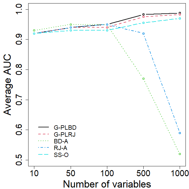
(a) $AUC$

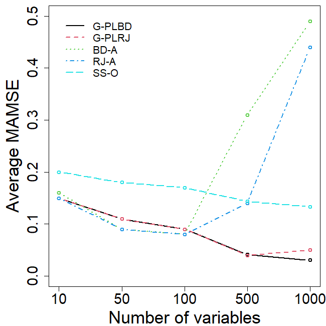
(b) $MAMSE$

Figure 1: Average AUC and average MAMSE by problem size for each algorithm. The average is taken over $50$ replications for $p\in\{10,50,100\}$ and $10$ replication for $p\in\{500,1000\}$. All replications performed on the cluster graph with $n=10p$ observations.

The AUC values of the algorithms (Figure 1(a)) are similar and improve with the problem size from around 0.92 for $p=10$ to 0.99 for $p=1000$. An exception to this is the BD-A and RJ-A algorithms. Their computational cost is so high for $p=500$ or $p=1000$ that they cannot provide decent AUC values within five days. The MAMSE values (Figure 1(b)) are also similar across algorithms and improve with the problem size from 0.15 for $p=10$ to 0.05 for $p=500$. Again, the BD-A and RJ-A algorithms are shown to not perform on high-dimensional problems. Another exception is the SS-O algorithm which has a worse MAMSE than the other algorithms. This is because the SS-O algorithm, more often than other algorithms, wrongly assigns an edge inclusion probability close to zero to an edge that is in the true graph. The accuracy of the algorithms is good overall, but astonishing at times. For example, for $p=500$ and using a threshold of $0.5$, the G-PLBD and G-PLRJ algorithms correctly identify around 90% of the edges, while wrongly identifying less than 0.1% of the non-edges.

The algorithms attain this remarkable accuracy with equally remarkable computational cost. Figure 2(a) shows that for $p=500$ the G-PLBD and G-PLRJ algorithms achieve excellent AUC values within $100$ seconds. Similarly, for thousand variable instances, the G-PLBD algorithm can achieve an AUC of $0.99$ within merely $100$ seconds.

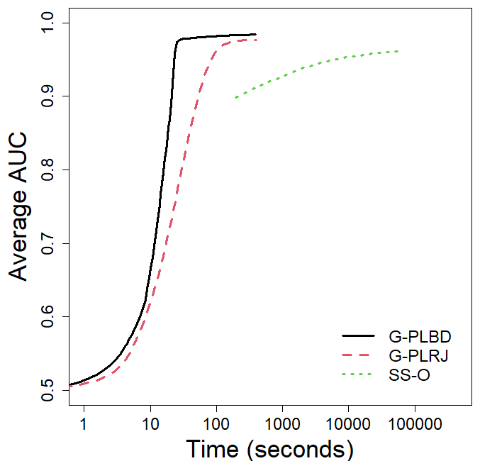
(a) $p=500$

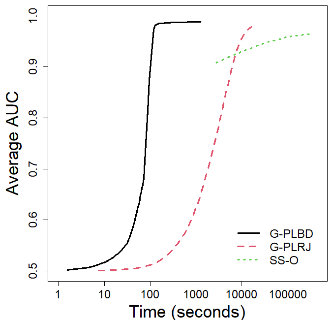
(b) $p=1000$

Figure 2: AUC over time (seconds) for the case $p=500$ (left) and $p=1000$ (right). The AUC shown is the average over 10 replications with $n=10p$ on the cluster graph.

In Figure 3, the median computational cost (20) is shown for all five algorithms for different values of $p$. For $p\in\{500,1000\}$ the BD-A and RJ-A algorithms have a computational cost of at least five days. These values are therefore not shown in the figure. Figure 3 shows that graphs with 50 and 100 variables can be solved to good AUC values within seconds by the G-PLBD, G-PLRJ, and SS-O algorithms. Even 500- and 1000-variable problems attain excellent AUC values within minutes for the G-PLBD algorithm.

(a) regular y-axis

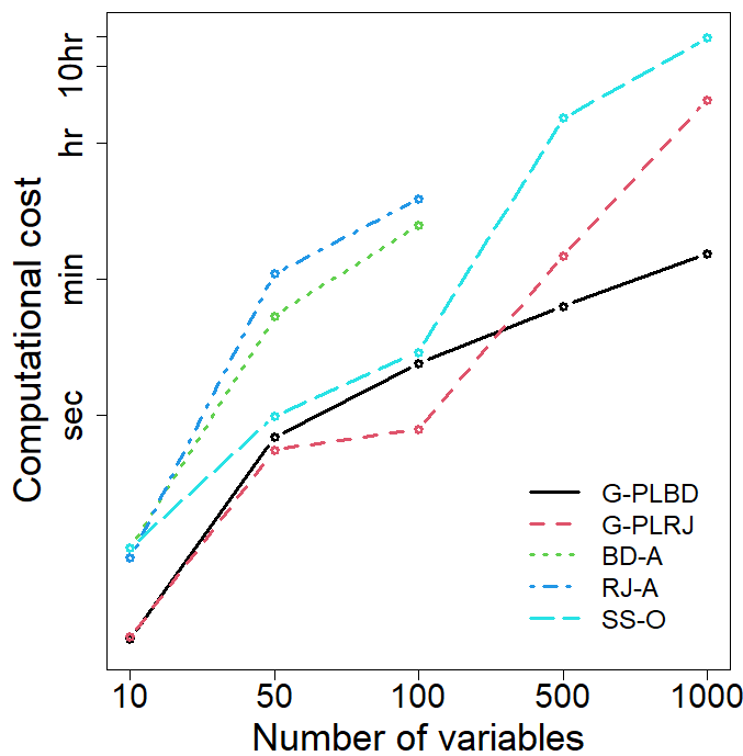
(b) logarithmic y-axis

Figure 3: The median computational cost $T$ (see Equation 20), by problem size for each algorithm. Both figures show the same data but with a regular y-axis (left) and a logarithmic-scale y-axis (right). The median is taken over $50$ replications for $p\in\{10,50,100\}$ and $10$ replication for $p\in\{500,1000\}$. All replications performed on the cluster graph with $n=10p$ observations.

So far, we have only considered instances where the number of observations $n$ is 10 times the number of variables ($n=10p$). As expected, when reducing the number of observations to $2p$ and $p$, we see a decrease in accuracy (see Figure 4). This effect is stronger for algorithms with few variables. The algorithms perform especially poorly for ten variable problems with few observations. In this case, the G-PLBD and G-PLRJ algorithms have an AUC of 0.65 and often produce edge inclusion matrices that are completely off.

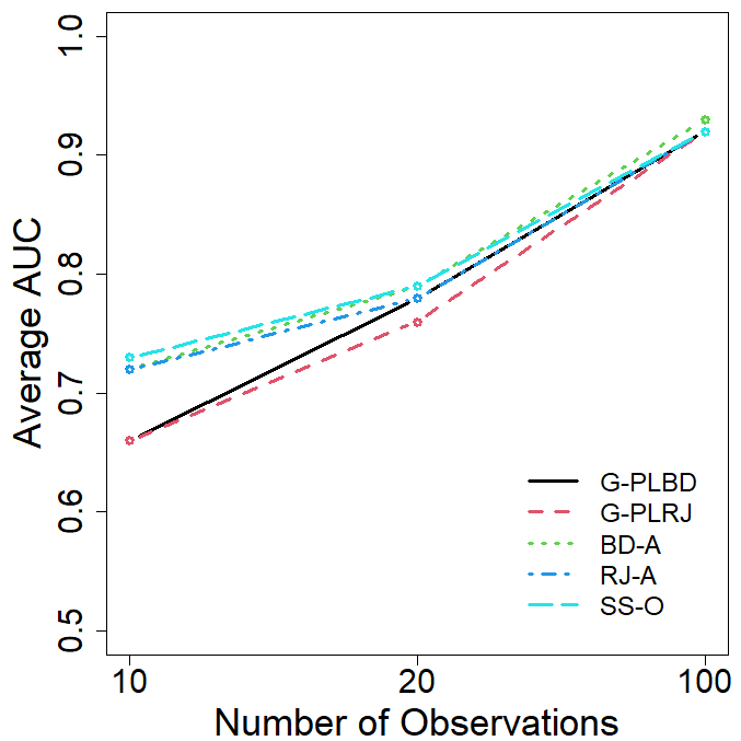
(a) $p=10$

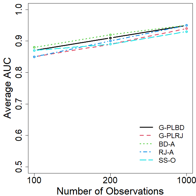
(b) $p=100$

Figure 4: Average AUC by the number of observations for each algorithm. For $p=10$ (left) and $p=100$ (right). The average is taken over $50$ replications. All replications were performed on the cluster graph.

Until now, we have only considered instances on the cluster graph. Figure 5 shows the average AUC and computational cost for different graph types for $p=100$ and $n=200$. In general, for low and high-dimensional problems, we observe a similar behaviour: the algorithms are less accurate and have a higher computational cost on the random graph. Edge density, or equivalently, graph sparsity, plays a big role in this. The random graphs have a density of $20\%$ whereas the scale-free and cluster graphs have densities that decrease with the dimension from $5\%$ at $p=50$ to less than $0.5\%$ for $p=1000$. The approximations used in the BD-A and RJ-A algorithms are more accurate for sparser graphs (Mohammadi et al., 2021). This also holds for the approximation in Equation (17) used by the G-PLBD and G-PLRJ algorithms. Moreover, moving one edge per iteration and starting at the empty graph, denser graphs take more iterations to approach. This becomes especially apparent for high-dimensional problems. At $p=1000$ for example, the G-PLRJ algorithm needs a whopping 200 mln MCMC iterations to reach an AUC of 0.8.

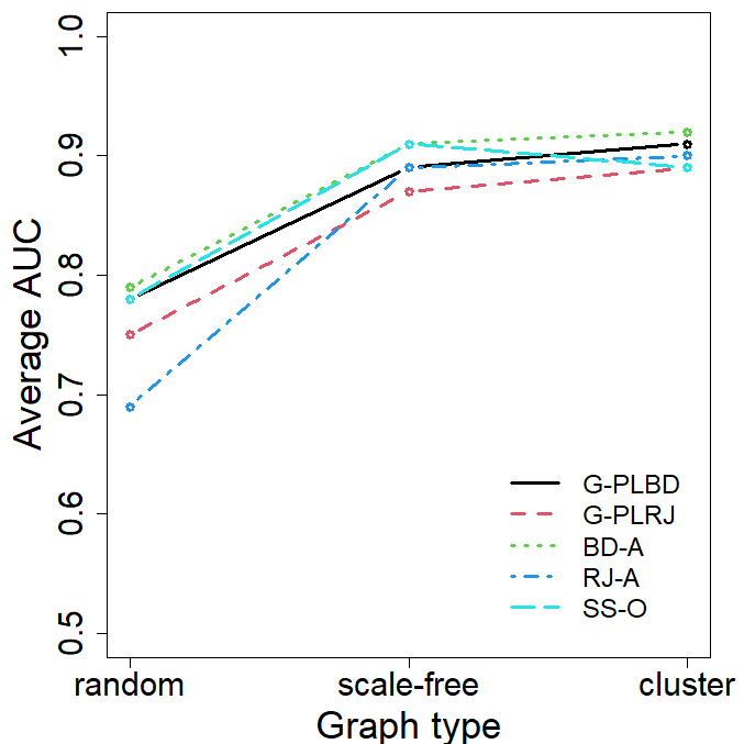
(a) AUC

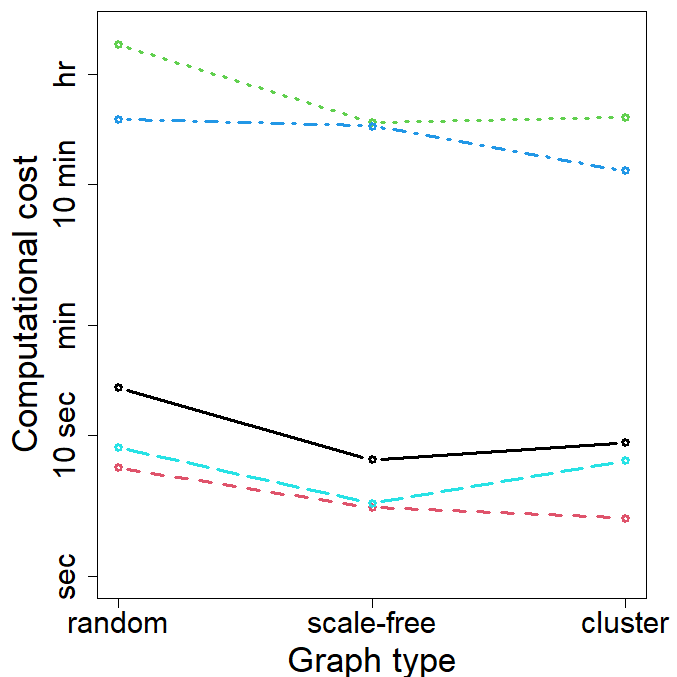
(b) Computational cost

Figure 5: Average AUC (left) and median computational cost (right) by graph type for each algorithm. For $p=100$ and $n=200$. The average and median are taken over $50$ replications.

The results in this section should be seen as a lower bound on the potential of Bayesian approaches due to the following reasons. First, all algorithms were run on one core. Allowing for more cores will improve computational efficiency even further, especially for algorithms that allow for parallelization like G-PLBD and BD-A. Second, we did not include a burn-in period. Appropriate burn-in periods are likely to lead to higher accuracies. Third, our prior graph structure did not reflect the true graph. The selected prior assigns a high probability to graphs with a density of around $20\%$. The cluster and scale-free graphs, however, have densities ranging from $0.5\%$ to $5\%$. A prior closer to the true graph is likely to yield better results. Lastly, we left out Bayesian algorithms that have been shown to perform well. The RJ-WWA is an MCMC algorithm that performs similarly to the BD-A algorithm (van den Boom et al., 2022). Moreover, the SS-EMGS, SS-BAGUS, H-LR, and H-WM algorithms are examples of approaches that do not have the computational burden of MCMC sampling but still provide good edge inclusion probabilities.

5 Conclusion and Future Research

In structure learning, Bayesian methods constitute a powerful alternative to frequentist ones. As multivariate systems in practice become more complex and connected, the Bayesian ability to incorporate model uncertainty becomes ever more essential. Meanwhile, the argument that the speed and simplicity of frequentist methods is superior, is waning as Bayesian methods have improved significantly in both aspects. Bayesian algorithms that provide accurate solutions to thousand variable problems within mere minutes are now a reality and easily accessible in software packages like BDgraph (Mohammadi et al., 2022) or ssgraph (Mohammadi, 2022). Yet, in the coming decade, Bayesian methods have the potential to become even faster, expand beyond the Gaussian case, and make more impact with its applications. This section conveys how.

First, new Markov chain Monte Carlo (MCMC) algorithms can increase the speed and feasible dimension of Bayesian structure learning. Mohammadi et al. (2023) showed the potential of MCMC algorithms that move only over the graph space, and not over the space of precision matrices. These algorithms, however, still only allow graphs to change at most one edge per MCMC iteration. It is an open question whether the detailed balance conditions in Equation (7) still hold when allowing changes of multiple edges. If true, this could lead to significant reduction in computation time. Similarly, van den Boom et al. (2022) showed the benefit of the informed proposal and delayed acceptance techniques for the reversible jump approach on the joint space of graphs and precision matrices. It remains to be shown whether algorithms on the graph space can benefit from the same techniques.

Wang (2015) introduced the spike and slab prior in Bayesian structure learning. He circumvented the calculation of the normalizing constant by putting its inverse in the prior of the graph. This leads to a fast algorithm, but creates a challenge when incorporating any knowledge of the graph structure in the prior of the graph. This raises two questions. (i) Could the normalizing constant of the spike and slab prior be approximated? (ii) Could G-Wishart algorithms on the joint space benefit from a similar trick? Furthermore, despite the success of the spike and slab algorithm (Wang, 2015), there are no MCMC algorithms with different spike and slab priors than Equation (15). Gan et al. (2019) do use a different spike and slab prior, but then design an expectation-maximization algorithm instead of an MCMC algorithm.

Second, moving away from the standard MCMC approach offers a promising and unexplored perspective to Bayesian structure learning. Dai et al. (2022) argue that Sequential Monte Carlo (SMC) methods remain under-used in statistics, despite several advantages. van den Boom et al. (2021) and Tan et al. (2017) show that the SMC approach works for Bayesian structure learning. However, their SMC algorithms cannot yet compete in terms of speed with the MCMC algorithms. Likewise, Nemeth & Fearnhead (2021) outline the benefits of the stochastic gradient MCMC (SGMCMC) method and Tan & Friel (2020) design an SGMCMC algorithm for exponential random graph models. As of now, however, no SGMCMC structure learning algorithm exists. Designing one, could advance Bayesian structure learning. Lastly, both the SS-EMGS (Li & McCormick, 2019) and SS-BAGUS (Gan et al., 2019) algorithms show that the expectation maximization (EM) approach produces accurate edge inclusion probabilities without the expensive search of the graph space necessary in MCMC algorithms. However, there is no comparison between MCMC algorithms and EM algorithms available and it remains unclear how the EM approach would scale to problems with dimension higher than $200$.

Third, recent improvements in structure learning in Gaussian graphical models (GGMs) could enhance algorithms beyond the general Gaussian case. The most apparent being the non-Gaussian case, in which the variables are not assumed to be multivariate normal, but instead are binary, ordinal, discrete or mixed. A popular technique in this case is Gaussian copula graphical models (GCGMs) (Dobra & Lenkoski, 2011). Using latent variables, GCGMs reformulate the non-Gaussian case into the familiar Gaussian problem. They then using existing GGM algorithms to perform structure learning. The state-of-the art algorithms discussed in this paper can therefore be directly applied to enhance non-Gaussian structure learning. This avenue, however, is barely investigated. Similarly, other related fields can benefit from the recent strides made in the general Gaussian case. They include multiple Gaussian graphical models (Tan et al., 2017), coloured Gaussian graphical models (Li et al., 2020) and graphical models with external network data (Jewson et al., 2022).

Lastly, the increase in the feasible dimension of Bayesian algorithms will enhance their applications. To discover the relationships between genes for example, Mohammadi & Wit (2015) reduce the available data set containing several thousands of genes to a mere one hundred genes to make the data feasible for their algorithm, potentially loosing valuable information. This kind of dimension reduction will be decreasingly necessary as Bayesian algorithms improve. Likewise, in neuroscience, the models of the brain no longer have to be simplified to just $100$ areas as in Dyrba et al. (2020). This could potentially improve the understanding of cognitive diseases like Alzheimer’s. The enhancements in Bayesian structure learning also open up new applications. Especially exciting but yet unexplored examples are graph neural networks and large language models, which both make use of dependency networks between a large amount of variables.

SUPPLEMENTARY MATERIAL

Table of MCMC iterations

that were used in the simulation study. Per algorithm, dimension, graph type, and amount of observations.

Github page

The scripts that produced the empirical results are available at https://anonymous.4open.science/r/Review-Paper-C869

References

- (1)
- Albert & Barabási (2002) Albert, R. & Barabási, A.-L. (2002), ‘Statistical mechanics of complex networks’, Rev. Mod. Phys. 74, 47–97.
- Anderson (2003) Anderson, T. (2003), An Introduction to Multivariate Statistical Analysis, Wiley-Interscience.
- Atay-Kayis & Massam (2005) Atay-Kayis, A. & Massam, H. (2005), ‘A Monte Carlo method for computing the marginal likelihood in non-decomposable Gaussian graphical models’, Biometrika 92(2), 317–335.
- Banerjee & Ghosal (2015) Banerjee, S. & Ghosal, S. (2015), ‘Bayesian structure learning in graphical models’, Journal of Multivariate Analysis 136, 147–162.
- Carvalho et al. (2007) Carvalho, C. M., Massam, H. & West, M. (2007), ‘Simulation of hyper-inverse Wishart distributions in graphical models’, Biometrika 94(3), 647–659.
- Chandra et al. (2022) Chandra, N. K., Mueller, P. & Sarkar, A. (2022), ‘Bayesian scalable precision factor analysis for massive sparse Gaussian graphical models’. Unpublished manuscript, arXiv: 2107.11316.
- Cheng & Lenkoski (2012) Cheng, Y. & Lenkoski, A. (2012), ‘Hierarchical Gaussian graphical models: Beyond reversible jump’, Electronic Journal of Statistics 6, 2309 – 2331.
- Dai et al. (2022) Dai, C., Heng, J., Jacob, P. E. & Whiteley, N. (2022), ‘An invitation to sequential monte carlo samplers’, Journal of the American Statistical Association 117(539), 1587–1600.
- Dawid & Lauritzen (1993) Dawid, A. P. & Lauritzen, S. L. (1993), ‘Hyper Markov laws in the statistical analysis of decomposable graphical models’, The Annals of Statistics 21(3), 1272–1317.
- Dempster (1972) Dempster, A. P. (1972), ‘Covariance selection’, Biometrics 28(1), 157–175.
- Dickey (1971) Dickey, J. M. (1971), ‘The weighted likelihood ratio, linear hypotheses on normal location parameters’, The Annals of Mathematical Statistics 42(1), 204 – 223.
- Dobra & Lenkoski (2011) Dobra, A. & Lenkoski, A. (2011), ‘Copula Gaussian graphical models and their application to modeling functional disability data’, The Annals of Applied Statistics 5(2A), 969–993.
- Dobra et al. (2011) Dobra, A., Lenkoski, A. & Rodriguez, A. (2011), ‘Bayesian inference for general Gaussian graphical models with application to multivariate lattice data’, Journal of the American Statistical Association 106(496), 1418–1433. PMID: 26924867.
- Drton & Maathuis (2017) Drton, M. & Maathuis, M. H. (2017), ‘Structure learning in graphical modeling’, Annual Review of Statistics and Its Application 4(1), 365–393.
- Dyrba et al. (2020) Dyrba, M., Mohammadi, R., Grothe, M. J., Kirste, T. & Teipel, S. J. (2020), ‘Gaussian graphical models reveal inter-modal and inter-regional conditional dependencies of brain alterations in alzheimer’s disease’, Frontiers in Aging Neuroscience 12.
- Gan et al. (2019) Gan, L., Narisetty, N. N. & Liang, F. (2019), ‘Bayesian regularization for graphical models with unequal shrinkage’, Journal of the American Statistical Association 114(527), 1218–1231.
- Giudici (1995) Giudici, P. (1995), ‘Bayes factors for zero partial covariances’, Journal of Statistical Planning and Inference 46(2), 161–174.
- Giudici & Castelo (2003) Giudici, P. & Castelo, R. (2003), ‘Improving Markov chain Monte Carlo model search for data mining’, Machine Learning 50, 127–158.
- Giudici & Green (1999) Giudici, P. & Green, P. J. (1999), ‘Decomposable graphical Gaussian model determination’, Biometrika 86(4), 785–801.
- Green (1995) Green, P. (1995), ‘Reversible jump Markov chain Monte Carlo computation and Bayesian model determination’, Biometrika 82(4), 711–732.
- Hinne et al. (2014) Hinne, M., Lenkoski, A., Heskes, T. M. & van Gerven, M. (2014), ‘Efficient sampling of Gaussian graphical models using conditional Bayes factors’, Stat 3, 326 – 336.
- Jewson et al. (2022) Jewson, J., Li, L., Battaglia, L., Hansen, S., Rossell, D. & Zwiernik, P. (2022), ‘Graphical model inference with external network data’. Unpublished manuscript, arXiv:2210.11107.
- Khondker et al. (2013) Khondker, Z., Zhu, H., Chu, H., Lin, W. & Ibrahim, J. (2013), ‘The Bayesian covariance lasso’, Statistics and its interface 6, 243–259.
- Kundu et al. (2018) Kundu, S., Mallick, B. & Baladandayuthapani, V. (2018), ‘Efficient Bayesian regularization for graphical model selection’, Bayesian Analysis 14, 449–476.
- Lauritzen (1996) Lauritzen, S. L. (1996), Graphical Models, Oxford University Press, Oxford, UK.
- Leday & Richardson (2018) Leday, G. & Richardson, S. (2018), ‘Fast Bayesian inference in large Gaussian graphical models’, Biometrics 75, 1288–1298.
- Lenkoski (2013) Lenkoski, A. (2013), ‘A direct sampler for G-Wishart variates’, Stat 2(1), 119–128.
- Lenkoski & Dobra (2011) Lenkoski, A. & Dobra, A. (2011), ‘Computational aspects related to inference in Gaussian graphical models with the G-Wishart prior’, Journal of Computational and Graphical Statistics 20(1), 140–157.
- Leppä-aho et al. (2017) Leppä-aho, J., Pensar, J., Roos, T. & Corander, J. (2017), ‘Learning Gaussian graphical models with fractional marginal pseudo-likelihood’, International Journal of Approximate Reasoning 83, 21–42.
- Letac & Massam (2007) Letac, G. & Massam, H. (2007), ‘Wishart distributions for decomposable graphs’, The Annals of Statistics 35(3), 1278 – 1323.
- Li & Zhang (2017) Li, F. & Zhang, X. (2017), ‘Bayesian lasso with neighborhood regression method for Gaussian graphical model’, Acta Mathematicae Applicatae Sinica, English Series 33, 485–496.
- Li et al. (2020) Li, Q., Gao, X. & Massam, H. (2020), ‘Bayesian model selection approach for coloured graphical Gaussian models’, Journal of Statistical Computation and Simulation 90(14), 2631–2654.
- Li et al. (2019) Li, Y., Craig, B. A. & Bhadra, A. (2019), ‘The graphical horseshoe estimator for inverse covariance matrices’, Journal of Computational and Graphical Statistics 28(3), 747–757.
- Li & McCormick (2019) Li, Z. R. & McCormick, T. H. (2019), ‘An expectation conditional maximization approach for Gaussian graphical models’, Journal of Computational and Graphical Statistics 28(4), 767–777.
- Maathuis et al. (2019) Maathuis, M., Drton, M., Lauritzen, S. & Wainwright, M. (2019), Handbook of Graphical Models, CRC Press, Boca Raton, Florida. Chapter 10.3.4.
- Massam et al. (2015) Massam, H., Li, Q. & Gao, X. (2015), ‘Bayesian precision matrix estimation for graphical Gaussian models with edge and vertex symmetries’, Biometrika 105(2), 371–388.
- Meinshausen & Bühlmann (2006) Meinshausen, N. & Bühlmann, P. (2006), ‘High-dimensional graphs and variable selection with the lasso’, The Annals of Statistics 34(3), 1436 –1462.
- Mohammadi et al. (2017) Mohammadi, A., Abegaz, F., van den Heuvel, E. & Wit, E. (2017), ‘Bayesian modelling of dupuytren disease by using Gaussian copula graphical models’, Journal of the Royal Statistical Society. Series C: Applied Statistics 66(3), 629–645.
- Mohammadi & Wit (2015) Mohammadi, A. & Wit, E. C. (2015), ‘Bayesian structure learning in sparse Gaussian graphical models’, Bayesian Analysis 10(1), 109 – 138.
- Mohammadi (2022) Mohammadi, R. (2022), ssgraph: Bayesian graph structure learning using spike-and-slab priors. R package version 1.15.
- Mohammadi et al. (2021) Mohammadi, R., Massam, H. & Letac, G. (2021), ‘Accelerating Bayesian structure learning in sparse Gaussian graphical models’, Journal of the American Statistical Association 0(0), 1–14.
- Mohammadi et al. (2023) Mohammadi, R., Schoonhoven, M., Vogels, L. & Birbil, I. S. (2023), ‘High-dimensional Bayesian structure learning in Gaussian graphical models using marginal pseudo-likelihood’. Unpublished manuscript , arXiv:2307.00127.
- Mohammadi et al. (2022) Mohammadi, R., Wit, E. & Dobra, A. (2022), BDgraph: Bayesian Structure Learning in Graphical Models using Birth-Death MCMC. R package version 2.72.
- Murray et al. (2006) Murray, I., Ghahramani, Z. & MacKay, D. (2006), ‘MCMC for doubly-intractable distributions’. In Proceedings of the 22nd Conference on Uncertainty in Artificial Intelligence 359-366.
- Natarajan et al. (2022) Natarajan, A., van den Boom, W., Odang, K. & De Iorio, M. (2022), ‘On a wider class of prior distributions for graphical models’. Unpublished manuscript, arXiv: 2205.04324 .
- Nemeth & Fearnhead (2021) Nemeth, C. & Fearnhead, P. (2021), ‘Stochastic gradient markov chain monte carlo’, Journal of the American Statistical Association 116(533), 433–450.
- Niu et al. (2021) Niu, Y., Pati, D. & Mallick, B. K. (2021), ‘Bayesian graph selection consistency under model misspecification.’, Bernoulli : Official journal of the Bernoulli Society for Mathematical Statistics and Probability 27(1), 637–672.
- Orchard et al. (2013) Orchard, P., Agakov, F. & Storkey, A. (2013), ‘Bayesian inference in sparse Gaussian graphical models’. Unpublished manuscript, arXiv: 1309.7311.
- Park & Casella (2008) Park, T. & Casella, G. (2008), ‘The Bayesian lasso’, Journal of the American Statistical Association 103(482), 681–686.
- Rajaratnam et al. (2008) Rajaratnam, B., Massam, H. & Carvalho, C. M. (2008), ‘Flexible covariance estimation in graphical Gaussian models’, Annals of Statistics 36, 2818–2849.
- Roverato (2002) Roverato, A. (2002), ‘Hyper inverse Wishart distribution for non-decomposable graphs and its application to Bayesian inference for Gaussian graphical models’, Scandinavian Journal of Statistics 29(3), 391–411.
- Sagar et al. (2021) Sagar, K., Sayantan, B., Jyotishka, D. & Anindya, B. (2021), ‘Precision matrix estimation under the horseshoe-like prior-penalty dual’. Unpublished manuscript, arXiv:2104.10750.
- Smith et al. (2023) Smith, J., Arashi, M. & Bekker, A. (2023), ‘A data driven Bayesian graphical ridge estimator’. Unpublished manuscript, arXiv:2210.16290.
- Stingo & Marchetti (2014) Stingo, F. & Marchetti, G. (2014), ‘Efficient local updates for undirected graphical models’, Statistics and Computing 25.
- Talluri et al. (2014) Talluri, R., Baladandayuthapani, V. & Mallick, B. (2014), ‘Bayesian sparse graphical models and their mixtures’, Stat 3(1), 109–125.
- Tan & Friel (2020) Tan, L. S. L. & Friel, N. (2020), ‘Bayesian variational inference for exponential random graph models’, Journal of Computational and Graphical Statistics 29(4), 910–928.
- Tan et al. (2017) Tan, L. S. L., Jasra, A., Iorio, M. D. & Ebbels, T. M. D. (2017), ‘Bayesian inference for multiple Gaussian graphical models with application to metabolic association networks’, The Annals of Applied Statistics 11(4), 2222 – 2251.
- Tierney & Kadane (1986) Tierney, L. & Kadane, J. B. (1986), ‘Accurate approximations for posterior moments and marginal densities’, Journal of the American Statistical Association 81(393), 82–86.
- van den Boom et al. (2022) van den Boom, W., Beskos, A. & Iorio, M. D. (2022), ‘The G-Wishart weighted proposal algorithm: Efficient posterior computation for Gaussian graphical models’, Journal of Computational and Graphical Statistics 31(4), 1215–1224.
- van den Boom et al. (2021) van den Boom, W., Jasra, A., De Iorio, M., Beskos, A. & Eriksson, J. (2021), ‘Unbiased approximation of posteriors via coupled particle Markov chain Monte Carlo’, Statistics and Computing 32(3), 1–19.
- Waldorp & Marsman (2022) Waldorp, L. & Marsman, M. (2022), ‘Relations between networks, regression, partial correlation, and the latent variable model’, Multivariate Behavioral Research 57(6), 994–1006. PMID: 34397314.
- Wang (2012) Wang, H. (2012), ‘Bayesian graphical lasso models and efficient posterior computation’, Bayesian Analysis 7(4), 867 – 886.
- Wang (2015) Wang, H. (2015), ‘Scaling it up: Stochastic search structure learning in graphical models’, Bayesian Analysis 10(2), 351–377.
- Wang & Li (2012) Wang, H. & Li, S. Z. (2012), ‘Efficient Gaussian graphical model determination under G-Wishart prior distributions’, Electronic Journal of Statistics 6, 168–198.
- Williams et al. (2018) Williams, D., Piironen, J., Vehtari, A. & Rast, P. (2018), ‘Bayesian estimation of Gaussian graphical models with projection predictive selection’. Unpublished manuscript, arXiv:1801.05725.
- Williams & Mulder (2020) Williams, D. R. & Mulder, J. (2020), ‘Bayesian hypothesis testing for Gaussian graphical models: Conditional independence and order constraints’, Journal of Mathematical Psychology 99, 102484.