Can extended Chaplygin gas source a Hubble tension resolved emergent universe ?

Abstract

In this paper, we attempt to explore the possibility of a obtaining a viable emergent universe scenario supported by a type of fluid known as the extended Chaplygin gas, which extends a modification to the equation of state of the well known modified Chaplygin gas by considering additional higher order barotropic fluid terms. We consider quadratic modification only. Such a fluid is capable of explaining the present cosmic acceleration and is a possible dark energy candidate. We construct a theoretical model of the emergent universe assuming it is constituted from such a fluid. It interestingly turns out that the theoretical constraints we obtain on the extended Chaplygin gas parameters from our emergent universe model are well in agreement with the observational constraint on these parameters from BICEP2 data. Our model is found to replicate the late time behaviour really well and reproduces $\Lambda$-CDM like behaviour, as evident from the analysis of the statefinder parameters. Moreover, the Hubble parameter analysis shows that for theoretically constrained values of the ECG parameters, the Hubble tension can be resolved yielding higher values of the present Hubble parameter $H_{0}$ in all possible cases. Also, the value of $H(z)$ at a redshift $z=2.34$ fits better than $\Lambda-CDM$ with recent observations in some cases. This leads us to the realization that such a fluid is not only a probable candidate for dark energy, but also sources an emergent universe unlike modified Chaplygin gas and the initial singularity problem can be resolved in a flat universe within the standard relativistic context.

1 Introduction

Over the years, the Big bang model has come to be accepted as the standard model of cosmology. The predictions of the Big bang model are compatible to quite a large extent with the presently available plethora of observational data. However, there are some problems with the standard Big bang model. Firstly, there is a ‘beginning’ of time, the point at which the field equations describing the spacetime are no longer capable of describing the physical situation due to presence of the “initial singularity[1].” As a consequence of this, the standard Big bang model can not answer the question about how the universe came into existence. There have been a number of efforts to resolve this initial singularity problem and to find an answer to the question regarding the coming into existense of the universe. Most physicists believe that at such an early phase of the universe, the energy densities were considerably high enough and the length scales involving the universe were comparable to or lower than the Planck length, making quantum gravity effects increasingly significant.

The main concern in dealing with the singularity problem is that there is no single consistent theory of Quantum Gravity (QG) at present. The two main theoretical setups in which a lot of efforts are being invested in this direction are the higher dimensional Superstring/ M- theories[3, 2] and the Loop Quantum Gravity (LQG)[4, 5]. Neither of the two scenarios have been fully developed till date, but there has been a lot of progress in both the fields in the last few decades. However, it is interesting to note that in a number of investigations involving both the setups, there have been a number of cosmological solutions in which the initial singularity is absent. In the LQG context, cosmological models involving a “regular bounce" have been proposed[6]. Such a bounce leads to a “cyclic” universe, where there are repeated non singular big bangs and big crunches. In the braneworld gravity context, which is a higher dimensional scenario inspired from the Superstring/ M- theories, similar cosmological solutions with non-singular bounce have been obtained[7], which may also be cyclic in nature by introducing a cosmological turnaround mechanism involving a homogenous scalar field[8]. In the context of $11$-dimensional M- theories, a “cyclic” picture of the universe has been obtained, where the Big bang is believed to be a collision between two dynamic braneworlds[9].

The second problem with the standard Big bang model is that it requires additional ingredients to explain the “dark sector” of the universe. The “dark sector” refers to the dark energy which is believed to be responsible for the presently observed accelerating phase of the universe[10, 11] and the dark matter whose effect can be realized via its gravitational interaction[12, 13]. In order to explain these effects, the standard relativistic Big bang scenario requires introduction of additional scalar fields capable of violating the strong energy condition like the quintessence[14, 15], tachyon[16] or phantom[17] fields, or exotic fluids like the Skyrme fluid[18]. Such a field is required to exist in the universe in addition to the “inflaton” scalar field responsible for the rapid accelerating expansion phase in the early universe realized through expoonential or power law type of scale factor. Inflation can also be realized via a tachyon field[19, 20]. For dark matter candidates, particles which have not yet been detected experimentally and are not predicted by the standard model of particle physics have to be taken into account. In an attempt to resolve these problems, there have been a number of cosmological models which make use of a modified Einstein-Hilbert action by considering additional terms in the Lagrangian of the geometry or the matter sector or both, contributing to non-conventional effects[21, 22, 23, 24]. The dark energy problem can also be resolved in the higher dimensional braneworld gravity setup[25, 26, 27] and the cyclic universe scenario obtained from the M- theory setup[9]. The simplest resolution is by considering a generalized Randall-Sundrum single brane model[28] which is characterized by perfect fluid bulk matter, resulting in an ‘effective’ fluid leading to accelerated expansion on the brane. In the cyclic picture[9], the inflationary phase is absent and a single scalar field governs all the phases of evolution of the universe from triggering the bounce to causing accelerated expansion. A cosmological bounce can also be obatained in the context of modified gravity[29, 30]. The dark matter problem can also be resolved in the context in the context of braneworld gravity, where the gravitational effect of any such hypothetical matter can be replaced by the higher dimensional braneworld effects.[31]

In the pure geometrical context, using conformal spacetime geometry, another cyclic cosmological model known as the Conformal cyclic cosmology has been proposed by Penrose[32]. The Emergent Universe (EU) scenario has been proposed by Ellis and Maartens[33] in 2004 and is a non-singular alternative to the Big bang resolving the initial singularity problem but it is different from the other scenarios in the context that there is no bounce or QG regime and also it is not a cyclic model. The scenario assumes an initial Einstein Static Universe (ESU), which corresponds to length scales greater than the Planck scale to avoid the QG regime and is subsequently followed by the standard inflationary and reheating phases. The EU scenario was originally proposed in a relativistic context, considering the presence of a positive curvature term in the Friedmann equations. Such an EU scenario[34] was also obtained in the relativistic context by considering a minimally coupled scalar field with a physically interesting potential to be the dominant source term in the early universe. An identical EU scenario[35] can also be obtained by adding a term quadratic in scalar curvature with a negative coupling parameter to the gravitaional Lagrangian. It was shown that the EU scenario can be realized with a spatial curvature term absent in the Friedmann equations[36], in the context of semi-classical Starobinsky gravity[37]. A generalized Equation of State (EoS) describing an EU[38] was found in the relativistic context, accomodating normal matter, exotic matter as well as dark energy. The EU scenario has been successfully studied in braneworld context[39] as well as the LQG context[40]. The EU scenario can also be realised in the framewrok of Einstein-Gauss-Bonnet gravity in four dimensions coupled with a dilaton field[41] as well as in the modified Gauss-Bonnet gravity[42].

A type of fluid known as “Chaplygin gas”, with its origin in string theories[43] had been used as a dark energy candidate to explain the late time acceleration of the universe[44, 45]. Such a fluid is characterized by the EoS $p=-\frac{B_{1}}{\rho}$, with $p$ and $\rho$ denoting the pressure and energy density, respectively in a comoving frame, while $B_{1}$ denotes the Chaplygin gas parameter. It is assumed that the energy density is positive and the constant $B_{1}>0$. However, for constructing a physically consistent cosmological model[46], the concerned EoS had to be modified to $p=-\frac{B_{1}}{\rho^{\alpha}}$, introducing an additional free parameter $\alpha$, such that $0\leq\alpha\leq 1$. This type of fluid is called the Generalized Chaplygin gas (GCG)[47, 48, 49, 50]. Initially it exhibits a dust like behaviour, but at late times it behaves asymptotically as a cosmological constant term, thus explaining the present acceleration of the universe. The EoS for GCG was further modified[51, 52, 53] for better correspondance with observational data, known as modified GCG[54, 55, 56, 57, 58]. The EoS for modified GCG has the form

$$p=A_{1}\rho-\frac{B_{1}}{\rho^{\alpha}},$$ (1)

where another additional constant parameter $A_{1}$ is introduced.

The Extended Chaplygin gas (ECG) EoS was proposed[59, 60, 61, 62, 63, 64, 65] to recover barotropic fluid having a quadratic or higher order EoS, which is basically a higher order generalization of the modified GCG at least upto the second order. The Van der Waals fluid is an alternative to the idea of a perfect fluid, that acts as the single source term in describing the evolution of the universe in both the matter dominated and present accelerating phases, identical to the Chaplygin gas family of fluids. It is also described a non-linear Equation of state[66] just like the Chaplygin gas family. The EoS for ECG may be written in general as

$$P=\sum_{n=1}^{\infty}A_{n}\rho^{n}-\frac{B_{1}}{\rho^{\alpha}}$$ (2)

Just like the other Chaplygin gas models, ECG is also used as a dark energy candidate to explain the present cosmic acceleration[59, 60, 61, 62]. Such models usually violate the strong energy condition of standard General Relativity (GR), which raises a possibility of violation of the null energy condition in the relativistic context. For obatining an EU scenario, it is likely that the null energy condition of GR must be violated[67]. So, it is worth investigating the possibility whether an EU scenario in the relativistic context is supported by such a dark energy candidate. Such an investigation has been performed for modified GCG[68], but it turns out that in order to make the EU scenario viable, the choice of the modified GCG parameters that are to be made are physically unrealistic. So, modified GCG does not support a viable EU scenario but since ECG incorporates higher order barotropic fluid extension of the modified GCG, it may be worth exploring whether this type of a fluid, suitable as a possible dark energy candidate can support an EU scenario or not. Moreover, ECG is known to admit bouncing and cyclic types of universes in the relativistic context[69].

In the following section, we shall consider the mathematical details of the possible EU scenario sourced by the ECG. In the final section we shall discuss the physical significance of the conclusions that can be inferred from our obtained results.

2 Mathematical model

Putting $n=2$ in Eq. (2), the EoS for Extended Chaplygin Gas (ECG) shall be upto the second order, which physically represents the quadratic barotropic EoS given by

$$P=A_{1}\rho+A_{2}\rho^{2}-\frac{B_{1}}{\rho^{\alpha}},$$ (3)

where $\rho$ represents the energy density, pressure is denoted by $P$ and $A_{1}$, $A_{2}$, $B_{1}$ and $\alpha$ denote the ECG parameters.

Here, for simplicity of the model, such that the number of free parameters be reduced and the energy density may be obtained analytically, the following realistic assumptions are made following the previous works[62, 70, 71]

$$\alpha=1$$

$$A_{1}=A_{2}-1$$ (4)

$$B_{1}=2A_{2}.$$

Conservation of energy-momentum tensor can be written as

$$\dot{\rho}+3H(\rho+P)=0,$$ (5)

where $H=\frac{\dot{a}}{a}$ denotes the Hubble parameter and $a$ is the scale factor.

Plugging in the EoS given by Eq. (3) into the conservation Eq. (5), we solve for the energy density in terms of the scale factor $a$, which turns out to be

$$\rho=1+\frac{2+\sqrt{5a^{30A_{2}}e^{\frac{3\pi}{2}}-1}}{a^{30A_{2}}e^{\frac{3\pi}{2}}-1}.$$ (6)

Our analysis is valid for all epochs of cosmic evolution such that we consider the early universe has considerably high energy densities ($\rho>>1$) and then the density gradually decreases before reaching an asymptotic value. For the late time $\rho<<1$. In order to obtain Eq. (6) we have used the approximations $tan^{-1}(\rho+1)\approx\frac{\pi}{2}$ for $\rho>>1$ and $tan^{-1}(\rho+1)\approx\frac{\pi}{4}$ for $\rho<<1$.

The first Friedmann equation is given as,

$$\rho=3H^{2}=3\bigg{(}\frac{\dot{a}}{a}\bigg{)}^{2}.$$ (7)

We choose $\kappa^{2}=8\pi G=1$.

From Eqs. (6) and (7), we obtain a solution for the scale factor $a$ as

$$a=\frac{\frac{2\sqrt{3}e^{\frac{15t}{\sqrt{3}A_{2}}}}{e^{\frac{15t}{A_{2}}-1}}-\frac{\sqrt{5}}{e^{\frac{15t}{A_{2}}-1}e^{\frac{3\pi}{4}}}}{\frac{2\sqrt{3}e^{\frac{15t}{\sqrt{3}A_{2}}}}{e^{\frac{15t}{A_{2}}-1}}-\frac{\sqrt{5}}{e^{\frac{15t}{A_{2}}-1}e^{\frac{3\pi}{4}}}-2}.$$ (8)

In obtaining the above solution, we have used the approximation $lna=\frac{1}{a-1}$. This approximation is justified as solution (6) approximately represents the late time behaviour particularly well. We shall compare this scale factor to the one used to describe an Emergent Universe (EU), which is also valid for all time scales, to establish a correspondance between the independent ECG parameter and the free parameter of the EU scale factor. That will allow us to obtain an estimate for the ECG parameters if ECG is to be considered as the constituent of an EU.

The expression of scale factor for the emergent Universe can be written of the form[36]

$$a(t)=a_{0}(10^{4}+e^{\frac{\sqrt{3}Bt}{2}})^{\frac{2}{3(A+1)}}.$$ (9)

As we can see, the above scale factor does not vanish as we go backwards in time to $t=0$ or beyond as in the standard Big bang picture. As a result there is no appearance of singularity in the Friedmann equations governing the dynamics of the universe. This physically means that the universe has no beginning at a particular point of time and the big bang is replaced by an ESU, whose length scales are large enough to avoid a quantum gravity regime.

If the universe with ECG as constituent is capable of behaving as an EU, then the scale factors obtained in Eqs. (8) and (9) must be identical. Comparing the two, expanding both the scale factors binomially and equating the coefficients for the first terms after expansion, we can obtain a correspondance between the free EU parameter $a_{0}$ and the independent ECG parameter $A_{2}$ as

$$a_{0}=\frac{2\sqrt{2}\times 10^{5}}{2e^{\frac{15}{A_{2}}-1}e^{\frac{3\pi}{4}}+2\sqrt{2}\times 10^{5}}$$ (10)

We know that the deceleration parameter $q(z)$ is defined as,

$$q(z)=\frac{\ddot{z}(1+z)}{\dot{z}^{2}}-2,$$ (11)

where $z$ denotes the redshift parameter.

The scale factor in Eq. (9) can be written in terms of the redshift $z$ as

$$z=\frac{1}{a}-1=\frac{1}{a_{0}\bigg{(}10^{4}+e^{\frac{\sqrt{3}Bt}{2}}\bigg{)}}-1$$ (12)

Taking first order derivative with respect to time, we get

$$\dot{z}=-\frac{B}{a_{0}\sqrt{3}\bigg{(}A+1\bigg{)}}\frac{e^{\frac{\sqrt{3}Bt}{2}}}{\bigg{(}10^{4}+e^{\frac{\sqrt{3}Bt}{2}}\bigg{)}^{\frac{3A+5}{3A+3}}}.$$ (13)

Writing down the above expression for $\dot{z}$ in terms of the redshift parameter $z$, we obtain

$$\dot{z}=-\frac{B}{\sqrt{3}\bigg{(}A+1\bigg{)}}\bigg{[}\frac{\big{(}z+1\big{)}^{\frac{2-3A-3A^{2}}{6(A+1)}}}{a_{0}^{\frac{4+9A+3A^{2}}{6(A+1)}}}-10^{4}\frac{\big{(}z+1\big{)}^{\frac{3A+5}{6(A+1)}}}{a_{0}^{\frac{3A+1}{6(A+1)}}}\bigg{]}$$ (14)

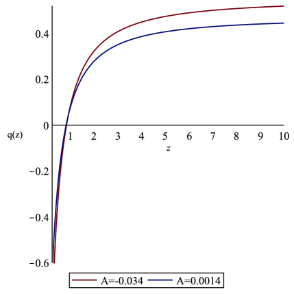
Figure 1: variation of deceleration parameter $q(z)$ with redshift $z$

Taking second order derivative of $z$ with respect to time, we get

$$\ddot{z}=\frac{\frac{B^{2}}{2(A+1)}e^{\frac{\sqrt{3}Bt}{2}}}{a_{0}\bigg{(}10^{4}+e^{\frac{\sqrt{3}Bt}{2}}\bigg{)}^{\frac{3A+5}{3A+3}}}-\frac{\frac{3B^{2}}{4}e^{\frac{\sqrt{3}Bt}{2}}\frac{(3A+5)^{2}}{3A+3}}{a_{0}\bigg{(}10^{4}+e^{\frac{\sqrt{3}Bt}{2}}\bigg{)}^{\frac{2(3A+4)}{3(A+1)}}}.$$ (15)

This can be expressed in terms of the redshift parameter $z$ as

$$\ddot{z}=\frac{3B^{2}}{6(A+1)}\bigg{[}\frac{(z+1)^{\frac{2-3A-3A^{2}}{6(A+1)}}}{a_{0}^{\frac{3A^{2}+9A+1}{6(A+1)}}}-10^{4}\frac{(z+1)^{\frac{3A+5}{6(A+1)}}}{a_{0}^{\frac{3A+1}{6(A+1)}}}\bigg{]}$$

$$-\frac{3B^{2}(3A+5)}{2(3A+3)^{2}}\bigg{[}\frac{(z+1)^{\frac{1}{3}}}{a_{0}^{\frac{2}{3}}}-\frac{2X10^{4}(z+1)^{\frac{3A+5}{6}}}{a_{0}^{\frac{1-3A}{6}}}+10^{8}a_{0}^{\frac{3A+1}{3}}(z+1)^{\frac{3A+4}{3}}\bigg{]}.$$ (16)

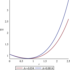
Figure 2: variation of jerk parameter $j(z)$ with redshift $z$

The observational constraints on the EU parameters $A$ and $B$ respectively are $-0.034\leq A\leq 0.0014$[72] and $0.003<B<0.5996$[73]. Using Eqs. (12), (14) and (16) in Eq.(11), it turns out that the deceleration parameter is independent of the second EU parameter $B$. So, we obtain the deceleration parameters for the lower and upper limits of $A$, respectively.

For the lower limit of $A$, we have

$$q(z)=\frac{1.45}{1-10^{4}a_{0}^{1.45}(z+1)^{1.45}}-0.55~{}[forA=-0.034]$$ (17)

and for the upper limit, we obtain

$$q(z)=\frac{1.5}{1-10^{4}a_{0}^{1.5}(z+1)^{1.5}}-0.47~{}[forA=0.0014]$$ (18)

The variation of the two deceleration parameters obtained above, along the redshift parameter $z$ have been plotted in Figure 1. The curve in red color represents the variation of the deceleration parameter with $z$ for the observationally constrained lower limit of EU parameter $A$, while the curve denoted in blue color represents the variation of deceleration parameter with $z$ for the observationally constrained upper limit of $A$. We shall discuss the physical consequence of the obtained plots in the concluding section.

The statefinder parameters[74] related to the late time behaviour are defined as

$$j=\frac{\ddot{H}}{H^{3}}-3q-2$$

$$s=\frac{j-1}{3(q-\frac{1}{2})},$$ (19)

where $j$ is known as the jerk parameter and $s$ is known as the snap parameter.

For the lower obsernational bound of $A$, we obtain the jerk and the snap parameters as follows

$$j(z)=\frac{4.205+2.1045\times 10^{4}a_{0}^{1.45}(1+z)^{1.45}}{\bigg{[}1-10^{4}a_{0}^{1.45}(z+1)^{1.45}\bigg{]}^{2}}-\frac{1.74}{1-10^{4}a_{0}^{1.45}(1+z)^{1.45}}+0.055,$$ (20)

and

$$s(z) = \frac{4.205+2.1045\times 10^{4}a_{0}^{1.45}(1+z)^{1.45}}{3\bigg{[}0.4+1.05\times 10^{4}a_{0}^{1.45}(1+z)^{1.45}\bigg{]}\bigg{[}1-10^{4}a_{0}^{1.45}(z+1)^{1.45}\bigg{]}}-\frac{1.74}{3\bigg{[}0.4+1.05\times 10^{4}a_{0}^{1.45}(1+z)^{1.45}\bigg{]}}$$ (21)

$$-\frac{0.945\bigg{[}1-10^{4}a_{0}^{1.45}(1+z)^{1.45}\bigg{]}}{\bigg{[}0.4+1.05\times 10^{4}a_{0}^{1.45}(1+z)^{1.45}\bigg{]}}.$$

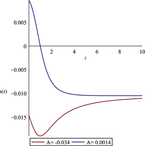
Figure 3: variation of snap parameter $s(z)$ with redshift $z$

For the higher observational bound on $A$, the jerk and snap parameters are evaluated as

$$j(z)=\frac{4.5+2.25\times 10^{4}a_{0}^{1.5}(1+z)^{1.5}}{\bigg{[}1-10^{4}a_{0}^{1.5}(z+1)^{1.5}\bigg{]}^{2}}-\frac{1.32}{1-10^{4}a_{0}^{1.5}(1+z)^{1.5}}-0.0282,$$ (22)

and

$$s(z) = \frac{4.5+2.25\times 10^{4}a_{0}^{1.5}(1+z)^{1.5}}{3\bigg{[}0.53+0.97\times 10^{4}a_{0}^{1.5}(1+z)^{1.5}\bigg{]}\bigg{[}1-10^{4}a_{0}^{1.5}(z+1)^{1.5}\bigg{]}}-\frac{1.32}{3\bigg{[}0.53+0.97\times 10^{4}a_{0}^{1.5}(1+z)^{1.5}\bigg{]}}$$ (23)

$$-\frac{1.0282\bigg{[}1-10^{4}a_{0}^{1.5}(1+z)^{1.5}\bigg{]}}{\bigg{[}0.53+0.97\times 10^{4}a_{0}^{1.5}(1+z)^{1.5}\bigg{]}}.$$

The variation of the jerk and snap parameters along the redshift for both values of $A$ have been plotted in Figures 2 and 3, respectively.

Finally, we obtain the Hubble parameter $H=\frac{\dot{a}}{a}$ in terms of the redshift $z$ as

$$H(z)=\frac{B}{\sqrt{3}\bigg{(}A+1\bigg{)}}\bigg{[}\frac{\big{(}z+1\big{)}^{-\frac{4+9A+3A^{2}}{6(A+1)}}}{a_{0}^{\frac{4+9A+3A^{2}}{6(A+1)}}}-10^{4}\frac{\big{(}z+1\big{)}^{-\frac{3A+1}{6(A+1)}}}{a_{0}^{\frac{3A+1}{6(A+1)}}}\bigg{]}$$ (24)

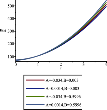
Figure 4: variation of Hubble parameter $H(z)$ (in km/sec/Mpc) with redshift $z$.

It is to be noted here that unlike the deceleration parameter, the Hubble parameter depends on both the EU parameters $A$ and $B$. There is also dependence on the ECG parameters which can in turn be expressed in terms of the single parameter $a_{0}$. The variation of the Hubble parameter along the redshift is given in Figure 4.

The EU parameter $B$ is absent in the deceleration parameter as the same dependence on $B$ appears in the numerator and denominator of the expression for the deceleration parameter, making it independent of $B$. The Hubble parameter is however found to depend on both the EU parameters $A$ and $B$. Also as mentioned in the manuscript, for obtaining analytic solutions, we have assumed some correspondence between the different ECG parameters following previous works, as a result of which the independent ECG parameter is $A_{2}$ which can be expressed in terms of the parameter $a_{0}$ from our analysis. We have used the plots of the variation of different parameters, namely the deceleration parameter, the jerk and snap parameters to constraint the value of the ECG parameters such that for observational bounds available on the EU parameters, we can obtain best fit for these parameters with the available observational data. The theoretical constraint on the ECG parameters obtained from our model in the process are confirmed with the Hubble parameter data as well and also with the previously obtained observational constraint from the BICEP2 data and they are found to be in very good agreement.

The physical explanation of the plots have been provided in the concluding section.

3 Discussion and Conclusion

In this paper, we have investigated the possibility of a viable EU scenario sourced by ECG. As discussed earlier, the different Chaplygin gas models finding their origin in the higher dimensional String theories are probable dark energy candidates, capable of explaining the late time accelerating behaviour of the universe. For obtaining such a behaviour in the relativistic context, it is expected that the strong energy condition as obtained from GR must be violated, which raises a possibility of violation of the null energy condition due to negative pressure. The violation of the null energy condition is essential for obtaining an EU scenario in the standard relativistic context in order to avert the initial singularity. So, it is worth investigating whether such a fluid supports an EU or not. Earlier investigation has revealed that the modified GCG does not support an EU for the realistic choice of the parameters concerned with the modified GCG[68]. However, the fluid we are considering here is an extension of the modified GCG EoS, allowing consideration of higher order barotropic fluid at least up to the quadratic term. Consideration of the additional term can possibly modify the fluid making it capable of supporting an EU, unlike the modified GCG, as it is found to support bouncing and cyclic types of regular cosmological solutions[69].

We have considered upto second order ECG term, physically representing the quadratic barotropic fluid. In order to obtain analytical mathematical solutions, we have assumed cetrain realistic correspondances between three of the free ECG parameters that have been applied in other investigations also[62, 70, 71]. The free parameter $\alpha$ involved in the EoS is assumed to be of unit magnitude without any loss of generality, as in the case of all the Chaplygin gas candidates[53, 62, 70, 71]. Vanishing divergence of the energy-momentum tensor yield the conservation equation and the energy density of the ECG is obtained from it. Using the first Friedmann equation, the scale factor is obtained using the late time approximation, as the solution for the energy density is valid for all epochs and represents the late time behaviour particularly well.

At this point we consider that ECG can support a viable EU scenario in order to impose some constraints on the ECG parameters from our theoretical model. So we consider the scale factor describing an EU to be identical to the scale factor that we have obtained by solving the Friedmann equation for a universe constituted out of ECG. Expanding both the scale factors binomially and equating the coefficients for the first terms, a relationship is obtained between the free parameter $a_{0}$ contained in the expression for the EU scale factor and the independent ECG parameter $A_{2}$, while the other two ECG parameters are expressed in terms of $A_{2}$ and $\alpha$ is of the order of unity. This allows us to constraint the ECG parameters $A_{1}$, $A_{2}$ and $B_{1}$ from our theoretical model of EU supported by ECG. If the theoretically obtained constraints on the upper and lower limits are in agreement with the constraints that have been obtained from the observational data[62], then it will justify our model and we shall argue that ECG supports a viable EU scenario.

It is known from observational findings that the present value of the deceleration parameter is $q\approx-0.57$ (SN+BAO datasets)[75] and the observationally obtained value of the redshift parameter at which the deceleration parameter flips sign from negative to positive, which means physically, the universe makes a transition from the accelerating to the decelerating phase (actually the reverse is hapenning as we are travelling forward in time), is typically $z\approx 0.8$[76]. While plotting the $q(z)$ versus $z$ curves for the observationally bound lower and upper limits of the EU parameter $A$ in Fig. 1, we are free to fix the EU parameter $a_{0}$. For fixing this parameter within a certain range, we find the best fit curve for $q(z)$ vs $z$, such that the present value of the deceleration parameter and the value of the redshift parameter at which the deceleration parameter vanishes are in close approximity to the observational values. As we see from the plot, for lower $A$, the rate of decrease of q is higher in the early era and then it flipped with the onset of the deceleration era, such that the time of flip is same in both the cases. We find from the best fit plot that in case of $A$=-0.034: for $z$=0, $q$=-0.61 and for $q$=0, $z$=0.82 and in case $A$=0.0014: for $z$=0, $q$=-0.59 and for $q$=0, $z$=0.83. For obtaining these best fit values, we obtain the theoretical constraint on $a_{0}$ as 0.0031$\leq a_{0}\leq$ 0.003753.

Now using Eq. (10), we may constrain the ECG parameter $A_{2}$ as 1.327$\leq A_{2}\leq$ 1.362 from our EU model. Using our earlier cosiderations in Eq. (4), we may also correspondingly constrain $A_{1}$ and $B_{1}$, respectively as 0.327$\leq A_{1}\leq$ 0.362 and 2.654$\leq B_{1}\leq$ 2.724. Thus, we obtain constraints on the three ECG parameters from our EU model by theoretically constraining the EU parameter $a_{0}$, making use of the observational constraint on the EU parameter $A$ and assuming that ECG can support an EU. These constraints on the ECG parameters obtained from our theoretical model are in very good agreement with the BICEP2 observational data which gives the observationally constrained limits on the ECG parameters as $1.2\leq A_{2}\leq 1.6$, $0.2\leq A_{1}\leq 0.6$ and $2.4\leq B_{1}\leq 3.2$[62]. Thus, we can see that the ECG parameters obtained from our theoretical model are within the observational range obtained from BICEP2 data and may be estimated more precisely, as the difference between the lower and upper bounds appear to be considerably smaller.

In order to analyze the late time behaviour of our obtained EU model more explicitly, we compute the jerk and the snap parameters. We evaluate the jerk and snap parameters for the obeservational lower and upper bounds of the EU parameter $A$ using the best fit value of the EU parameter $a_{0}$, which we had obtained to evaluate the theoretical constraints on the ECG parameters. As we can see from Fig. 2, the present value of the jerk parameter at redshift $z=0$ that we obtain from our theoretical model is very close to 1 for both values of $A$, and as we go back in time, the jerk parameter first decreases and then increases but the rate of increase is higher for the upper bound (higher value) of $A$. This behaviour is in agreement with the $\Lambda$-CDM (cold dark matter) model. For the snap parameter, we see from Fig. 3 that for the higher $A$, the snap parameter presently has a vanishingly small positive value and as we go back in time, the parameter reduces and changes sign to a negative value. For the lower value of $A$, presently it has a very tiny negative value and first decreases and then increases as we go back in time. The $\Lambda$-CDM model predicts the present values of the jerk and snap parameters to be 1 and 0, respectively. As we see, our model reproduces this value to a close approximation. Thus the late time behaviour is also well predicted by our EU model supported by an ECG.

We have also obtained an expression for the Hubble parameter in terms of the redshift and plotted its variation. We have plotted the variation for all possible combinations of the lower and upper observational bounds of the EU parameters $A$ and $B$. The parameter $a_{0}$ which encodes the information regarding the ECG parameters is chosen for the best fit of the curve and the corresponding ECG parameter $A_{2}$ turns out to have a value 1.35 for obtaining the best fit of the Hubble variation to observational data[77, 78]. This value of the ECG parameter is within our obtained range from the analysis of the other parameters and hence in support of our model. We see from Fig. 4 that as the redshift increases, the Hubble parameter also increases as expected. We obtain the values of $H(z)$ at two particular redshifts, namely $z=0$ (denoting the value of the Hubble parameter at present time $H_{0}$) and $z=2.34$ (in km/sec/Mpc), to tally with observational data. For the first choice of EU parameters $A=-0.034$ and $B=0.003$, we get $H_{0}=73.254$ and $H(z=2.34)=233.7$. For $A=-0.034$ and $B=0.5996$, we get $H_{0}=72.302$ and $H(z=2.34)=240.2$. For $A=0.014$ and $B=0.003$, we get $H_{0}=74.206$ and $H(z=2.34)=231$. For $A=0.014$ and $B=0.5996$, we get $H_{0}=70.029$ and $H(z=2.34)=244.2.$ The observed data suggests $H_{0}=73.24\pm 1.74km/sec/Mpc$[77] and $H(z=2.34)=222\pm 7km/sec/Mpc\cite[cite]{[\@@bibref{}{Debulac}{}{}]}$. There is a slight discrepancy with the $\Lambda-CDM$ estimated values of $H_{0}=67km/sec/Mpc$ and $H(z=2.34)=238km/sec/Mpc$. For the present values of the Hubble parameter, our model provides a better fit for the observational data for all four possible combinations of the upper and lower EU parameter bounds, thus resolving the Hubble tension. For the value at higher redshift, our model predicts a better fit in two cases while the fit is worse compared to $\Lambda-CDM$ estimation in the other two cases.

Hence, we make the claim that the ECG fluid does source an EU scenario consistent with the observational data unlike modified GCG, besides being a probable dark energy candidate as evident from the fact that it replicates the late time behaviour very well. This characteristic of supporting an EU, unlike modified GCG, can be interpreted to be a result of the modification arising from the higher order quadratic barotropic fluid term in the modified EoS, due to which the null energy condition (NEC) can be violated while in case of modified GCG only the strong energy condition is violated. We conclude that ECG is more open to exploring different cosmological scenarios than the previous Chaplygin gas candidates as it supports a non-singular universe owing to NEC violation besides reproducing a $\Lambda$-CDM like behaviour and at late times. The most important perspective is that the initial singularity problem can be resolved in a standard relativistic context for a flat universe and the obtained late time cosmology from the EU model is in good agreement with observational data, at per with or even better than the standard $\Lambda-CDM$ model in some cases.

4 Appendix

We present a few steps of the derivation of the solution (6) from the conservation equation (5). The solution is obtained under some approximations namely $tan^{-1}(\rho+1)\approx\frac{\pi}{2}$ for $\rho>>1$ (early universe) and $tan^{-1}(\rho+1)\approx\frac{\pi}{4}$ for $\rho<<1$ (late times). If these approximations are invoked, then the solution (6) will satisfy the differential equation (5). A few steps towards obtaining the solution are presented below.

On integrating both sides of the differential equation (5) and simplifying, we are left with

$$lna=\frac{1}{30A_{2}}ln{\bigg{[}\frac{\rho^{2}+2\rho+2}{\rho^{2}-2\rho+1}\bigg{]}}-\frac{\pi}{20A_{2}}+C^{\prime},$$ (25)

where $C^{\prime}$ is a constant of integration which we assume to be zero for simplicity.

Upon further simplification, this may be expressed as a quadratic equation of $\rho$ having the form

$$(a^{30A_{2}}-e^{-\frac{3\pi}{2}})\rho^{2}-2(a^{30A_{2}}+e^{-\frac{3\pi}{2}})\rho+(a^{30A_{2}}-2e^{-\frac{3\pi}{2}})=0$$ (26)

On taking the positive root solution, we get

$$\rho=1+\frac{2+\sqrt{2a^{30A_{2}}e^{\frac{3\pi}{2}}+1+3a^{30A_{2}}e^{\frac{3\pi}{2}}-2}}{a^{30A_{2}}e^{\frac{3\pi}{2}}-1}$$ (27)

which on simplification gives Equation (6).

5 Acknowlwdgement

MK and BCP is thankful to the Inter-University Centre for Astronomy and Astrophysics (IUCAA),Pune, India for providing the Visiting Associateship under which a part of this work was carried out. RS is thankful to the Govt. of West Bengal for financial support through SVMCM scheme.

References

- [1] S. W. Hawking and G. F. R. Ellis, Astrophys. J. 152 (1968) 25.
- [2] B. Zwiebach, A First Course in String Theory (Cambridge University Press, 2004).
- [3] J. Polchinski, String Theory, Vol. 2, Superstring Theory and Beyond (Cambridge University Press, 1998).
- [4] R. Gambini and J. Pullin, A First Course in Loop Quantum Gravity (Oxford University Press, 2011)
- [5] C. Rovelli, Living Rev. Rel. 11 (2008) 5.
- [6] M. Bojowald, R. Maartens and P. Singh, Phys. Rev. D 70 (2004) 083517.
- [7] Y. Shtanov and V. Sahni, Phys. Lett. B 557 (2003) 1.
- [8] V. Sahni and A. Toporensky, Phys. Rev. D 85 (2012) 123542.
- [9] P. J. Steinhardt and N. Turok, Phys. Rev. D 65 (2002) 126003.
- [10] A.G. Riess et al., Astron. J. 116 (1998) 1009.
- [11] S. Perlmutter et al., Astrophys. J. 517 (1999) 565.
- [12] F. Zwicky, Helvetica Physica Acta 6 (1933) 110.
- [13] V. C. Rubin and Jr. W. K. Ford, Astrophys. J. 159 (1970) 379.
- [14] E. J. Copeland, A. R. Liddle and D. Wands, Phys. Rev. D 57 (1998) 4686.
- [15] I. Zlatev, L. M. Wang and P. J. Steinhardt, Phys. Rev. Lett. 82 (1999) 896.
- [16] P. P. Avelino, L. Losano and J.J. Rodrigues, Phys. Lett. B 699 (2011) 10.
- [17] M. P. Dabrowski, T. Stachowiak, and M. Szydlowski, Phys. Rev. D 68 (2003) 103519.
- [18] R. Sengupta, B. C. Paul and P. Paul, Pramana – J. Phys. 96 (2022) 114.
- [19] N. Bilic et al., JCAP 08 (2019) 034.
- [20] R. Sengupta, P. Paul, B. C. Paul, S. Ray, Int. Jour. of Mod. Phys. D 28 (2019) 1941010.
- [21] S. Nojiri, S. D. Odintsov and P. V. Tretyakov, Phys. Lett. B 651 (2007) 224.
- [22] S. Nojiri, S. D. Odintsov and O. G. Gorbunova, J. Phys. A 39 (2006) 6627.
- [23] M. Szydlowski, A. Kurek and A. Krawiec, Phys. Lett. B 642 (2006) 171.
- [24] D. Huterer and E. V. Linder, Phys. Rev. D 75 (2007) 023519.
- [25] G. Dvali, G. Gabadadze and M. Porrati, Phys. Lett. B 485 (2000) 208.
- [26] V. Sahni and Y. Shtanov, JCAP 11 (2003) 014.
- [27] S. Chakraborty, A. Banerjee and T. Bandyopadhyay, arXiv:0707.0199.
- [28] L. Randall and R. Sundrum, Phys. Rev. Lett. 83 (1999) 4690.
- [29] S. D. Odintsov, V. K. Oikonomou and E. N. Saridakis, Annals of Physics 363 (2015) 141.
- [30] S. K. Tripathy, B. Mishra, S. Ray and R. Sengupta, Chinese Journal of Physics 71 (2021) 610.
- [31] S. Pal, S. Bharadwaj and S. Kar, Phys.Lett. B 609 (2005) 194.
- [32] R. Penrose, AIP Conference Proceedings 1446 (2012) 233.
- [33] G F. R. Ellis and R. Maartens, Class. Quant. Grav. 21 (2004) 223.
- [34] G F. R. Ellis, J. Murugan and C. G. Tsagas, Class. Quant. Grav. 21 (2004) 233.
- [35] D. J. Mulryne, R. Tavakol, J. E. Lidsey and G. F. R. Ellis, Phys. Rev. D 71 (2005) 123512.
- [36] S. Mukherjee, B. C. Paul, S. D. Maharaj and A. Beesham, arXiv:gr-qc/0505103 (2005).
- [37] A. A. Starobinsky, Phys. Letts. B 91 (1980) 99.
- [38] S. Mukherjee, B. C. Paul, N. Dadhich, S. D. Maharaj and A. Beesham, Class. Quant. Grav. 23 (2006) 6927.
- [39] A. Banerjee, T. Bandyopadhyay and S. Chakraborty, Grav. Cosmol. 13 (2007) 290.
- [40] B. Paik, M. Y. Khlopov, M. Kalam and S. Ray, Physics of the Dark Universe 32 (2021) 100823.
- [41] B. C. Paul and S. Ghosh, Gen. Rel. and Grav. 42 (2010) 795.
- [42] B. C. Paul, S. D. Maharaj and A. Beesham, arXiv:2008.00169.
- [43] M. Bordemann, J. Hoppe, Phys. Lett. B 317 (1993) 315.
- [44] V. Gorini, A. Kamenshchik and U. Moschella, Phys. Rev. D 67 (2003) 063509.
- [45] U. Alam, V. Sahni, T. D. Saini and A. A. Starobinsky, Mon. Not. Roy. Astron. Soc. 344 (2003) 1057.
- [46] M. C. Bento, O. Bertolami and A. A. Sen, Phys. Rev. D 66 (2002) 043507.
- [47] A. R. Amani and B. Pourhassan, Int. Jour. of Theoretical Phys. 52 (2013) 1309.
- [48] H. Saadat and B. Pourhassan, Int. Jour. of Theoretical Phys. 52 (2013) 3712.
- [49] H. Saadat and B. Pourhassan, Int. Jour. of Theoretical Phys. 53 (2014) 1168.
- [50] A. R. Amani and B. Pourhassan, Int. Jour. of Geom. Methods in Mod. Phys. 11 (2014) 1450065.
- [51] U. Debnath, A. Banerjee, and S. Chakraborty, Class. Quant. Grav. 21 (2004) 5609.
- [52] Y-B. Wu et al., Mod. Phys. Lett. A 30 (2015) 1550005.
- [53] S. Ray et al., Int. Jour. of Mod. Phys. D 30 (2021) 2150093.
- [54] H. Saadat and B. Pourhassan, Astrophys. Space Sci. 343 (2013) 783.
- [55] H. Saadat and B. Pourhassan, Astrophys. Space Sci. 344 (2013) 237.
- [56] B. Pourhassan, Int. Jour. of Mod. Phys. D 22 (2013) 1350061.
- [57] J. Sadeghi, B. Pourhassan, M. Khurshudyan and H. Farahani, Int. Jour. of Theoretical Phys. 53 (2014) 911.
- [58] E.O. Kahya, B. Pourhassan and S. Uraz, Phys. Rev. D 92 (2015) 103511.
- [59] B. Pourhassan and E.O. Kahya, Advances in High Energy Physics 2014 (2014) 231452.
- [60] E.O. Kahya, M. Khurshudyan, B. Pourhassan and R. Myrzakulov, A. Pasqua, Euro. Phys. Jour. C 75 (2015) 43.
- [61] B. Pourhassan and E.O. Kahya, Results in Phys. 4 (2014) 101.
- [62] E. O. Kahya and B. Pourhassan, Astrophys. Space Sci. 353 (2014) 677.
- [63] J. Sadeghi, H. Farahani, B. Pourhassan, Eur. Phys. J. Plus 130 (2015) 84.
- [64] B. Pourhassan, Canadian Jour. of Phys. 94 (2016) 659.
- [65] B. Pourhassan, H. Farahani, S. Upadhyay, New Astronomy 86 (2021) 101569.
- [66] M. Biswas, S. Maity and U. Debnath, Jour. of Holography Applications in Physics, 1(1) (2021) 71.
- [67] M. Zhu and Y. Zheng, JHEP 11 (2021) 163.
- [68] S. Dutta, S. Mukerji and S. Chakraborty, Advances in High Energy Physics, 2016 Article ID 7404218 (2016).
- [69] A. Salehi, Phys. Rev. D 94 (2016) 123519.
- [70] B. Pourhassan, Physics of the Dark Universe 13 (2016) 132.
- [71] E. O. Kahya and B. Pourhassan, Mod. Phys. Lett. A Vol. 30, 13 (2015) 1550070.
- [72] B.C. Paul, P. Thakur and S. Ghose, Mon. Not. Royal Astron. Society 407 (2010) 15.
- [73] B.C. Paul, P. Thakur and S. Ghose, Mon. Not. Royal Astron. Society 413 (2011) 686.
- [74] V. Sahni et. al., J. Exp. Theor. Phys. Lett., 77 (2003) 201.
- [75] S. K. J. Pacif, S. Arora and P. K. Sahoo, Phys. Dark Universe 32 (2021) 100804.
- [76] A. Al Mamon and K. Bamba, Eur. Phys. J. C 78 (2018) 862.
- [77] Riess et al., ApJ 826 (2016) 56.
- [78] Debulac et al., A and A 574 (2015) A59.