Euler-Bernoulli beams with contact forces: existence, uniqueness, and numerical solutions

Abstract

In this paper, we investigate the Euler-Bernoulli fourth-order boundary value problem (BVP) $w^{(4)}=f(x,w)$, $x\in[a,b]$, with specified values of $w$ and $w^{\prime\prime}$ at the end points, where the behaviour of the right-hand side $f$ is motivated by biomechanical, electromechanical, and structural applications incorporating contact forces. In particular, we consider the case when $f$ is bounded above and monotonically decreasing with respect to its second argument. First, we prove the existence and uniqueness of solutions to the BVP. We then study numerical solutions to the BVP, where we resort to spatial discretization by means of finite difference. Similar to the original continuous-space problem, the discrete problem always possesses a unique solution. In the case of a piecewise linear instance of $f$, the discrete problem is an example of the absolute value equation. We show that solutions to this absolute value equation can be obtained by means of fixed-point iterations, and that solutions to the absolute value equation converge to solutions of the continuous BVP. We also illustrate the performance of the fixed-point iterations through a numerical example.

Keywords— Euler-Bernoulli beams; Contact forces; Boundary value problems; Vocal folds; Microswitches; Beams on elastic foundations.

Introduction

In biomechanical applications, especially those related to voice production, contact forces arise naturally. For example, prior to and during voice production, the vocal folds (VFs) typically experience contact forces as they touch each other and/or collide. In general, and due to the emergence of contact forces and the complexity of the air flow interacting with the VFs during phonation, voice-related models are typically non-smooth. Despite the non-smoothness, numerical solvers that are designed primarily for smooth systems are often implemented when solving phonation equations. Moreover, the nature of solutions (e.g., existence, uniqueness, smoothness, etc.) to these non-smooth equations is usually dismissed as they tend to be analytically intractable, and the effectiveness of numerical solvers (i.e., convergence) are tested only empirically. Consequently, a major portion of the numerical studies of voice-related models lack mathematical rigor, with no guarantees regarding the correctness and accuracy of the reported numerical solutions. Therefore, it is important to investigate voice-related models mathematically, when feasible, and elucidate the nature of their analytical and numerical solutions.

The VFs are often modelled as elastic structures, with incorporated repulsive contact forces that take place when the folds touch each other, with forces being proportional to the degree of compression (see, e.g., [1, 2, 3]). A very simple abstraction of the VFs, which is more suited for scenarios concerning static configurations (e.g., posturing), relies on considering one of the VFs as an Euler-Bernoulli beam that experiences contact spring forces, and assuming the other fold to be an image of the first one with respect to the contact plane; see Figure 1.

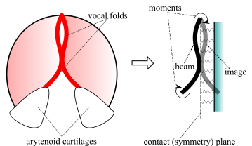
Figure 1: Modelling the configuration of the vocal folds (left) using a beam with spring forces resembling contact (right).

That is, the VF configuration, presented by the deflection function $v$, satisfies the differential equation $\beta v^{(4)}=F_{s}(s)$, where $\beta$ is the bending stiffness and $F_{s}(s)$ is the contact spring force (per unit length), in addition to complementary boundary conditions (BCs) in terms of displacements and moments at the end points of the beam. Such an abstraction is analytically tractable, allowing rigorous mathematical investigation that we pursue in this work. In fact, such modelling framework has been adopted to understand curved VF configurations under different laryngeal conditions [6]. In addition to biomechanical applications, similar beam models with contact forces arise in electromechanical systems, such as micoswithches [7, 8], and civil structural applications, such as beams on elastic foundations [9, 10, 11, 12]. Therefore, due to their relevance in different applications, we study mathematically Euler-Bernoulli beams with contact forces in terms of solution existence and uniqueness and the properties of numerical solutions, especially those resulting from finite difference approximations.

The organization of this paper is as follows. Necessary preliminaries and notations are provided in Section 1, problem formulation and associated assumptions are introduced in Section 2, relevant findings from the literature are presented in Section 3, existence and uniqueness results and their proofs are presented in Section 4, the discretized boundary value problem and the existence and uniqueness of its solutions are discussed in Section 5 with a further consideration of the numerical solutions in the case of a piecewise linear right-hand side in Section 6, and the study is concluded in Section 7.

1 Preliminaries

Let $\mathbb{R}$, $\mathbb{R}_{+}$, $\mathbb{Z}$, and $\mathbb{Z}_{+}$ denote the sets of real numbers, nonnegative real numbers, integers, and nonnegative integers, respectively, and $\mathbb{N}=\mathbb{Z}_{+}\setminus\{0\}$. Let $[a,b]$ denote the closed interval with end points $a$ and $b$, and $[a;b]$ stands for its discrete counterpart ($[a;b]=[a,b]\cap\mathbb{Z}$). For $x\in\mathbb{R}^{n}$, we define $|x|=(|x_{1}|,\ldots,|x_{n}|)$. Given $x,y\in\mathbb{R}^{n}$, $x\leq y\Leftrightarrow x_{i}\leq y_{i}~{}\forall i\in[1;n]$. In this work, $\|\cdot\|_{p}$ denotes any $p$-norm on $\mathbb{R}^{n}$ with $p\in[1,\infty]$, e.g., $\|x\|_{\infty}=\max_{i\in[1;n]}|x_{i}|,~{}x\in\mathbb{R}^{n}$. Given $A\in\mathbb{R}^{n\times m}$, $\|A\|_{p}$ denotes the matrix norm induced by $\|\cdot\|_{p}$ (e.g., $\|A\|_{\infty}=\max_{i\in[1;n]}\sum_{j=1}^{m}|A_{i,j}|$, $\|A\|_{1}=\max_{j\in[1;m]}\sum_{i=1}^{n}|A_{i,j}|$ ). Given $A\in\mathbb{R}^{n\times n}$, $\sigma(A)$ denotes the set of eigenvalues of $A$. If $A\in\mathbb{R}^{n}$ is symmetric ($A=A^{\intercal}$), then $\lambda_{i}(A)$ denotes the $i^{\mathrm{th}}$ eigenvalue of $A$ (which is real), such that $\lambda_{i}(A)\leq\lambda_{i+1}(A),~{}i\in[1;n-1].$ The identity map defined on $\mathbb{R}^{n}$ is denoted by $\operatorname{id}$, where the dimension will be clear from the context. Integration of single-valued functions $f\colon X\rightarrow Y$ is always understood in the sense of Lebesgue. $C[a,b]$ denotes the Banach space of continuous functions $f:[a,b]\rightarrow\mathbb{R}$ equipped with the uniform norm $\|f\|_{C[a,b]}\mathrel{:=}\sup_{x\in[a,b]}|f(x)|$. Given $p,q\in C[a,b]$, $p\leq q\Leftrightarrow p(x)\leq q(x)~{}\forall x\in[a,b]$. Let $\mathrm{Lip}_{k}[a,b]$, where $k\in\mathbb{R}_{+}$, denotes the space of Lipschitz continuous functions $f:[a,b]\rightarrow\mathbb{R}$, with Lipschitz constants less than or equal to $k$; that is $f\in\mathrm{Lip}_{k}[a,b]\Leftrightarrow|f(x)-f(y)|\leq k|x-y|~{}\forall x,y\in[a,b].$ Finally, $C^{k}[a,b]$, where $k\in\mathbb{N}$, denotes the space of $k$-times continuously differentiable functions $f:[a,b]\rightarrow\mathbb{R}$ (derivatives at $a$ and $b$ are one-sided).

2 Problem formulation

As a generalization of the Euler-Bernoulli model with contact discussed in the introduction, we consider the fourth-order BVP over the compact interval $[a,b]$ with respect to the function $w:[a,b]\rightarrow\mathbb{R}$:

$$w^{(4)}=f(x,w), ~{}x\in[a,b],$$ (1a)

$$w(a)=\alpha_{1},~{}w(b)=\alpha_{2}, ~{}w^{\prime\prime}(a)=\beta_{1},~{}w^{\prime\prime}(b)=\beta_{2},$$ (1b)

where $\alpha_{1},\alpha_{2},\beta_{1},\beta_{2}\in\mathbb{R}$ are specified boundary values, and $f:[a,b]\times\mathbb{R}\rightarrow\mathbb{R}$ satisfies the following set of properties:

$$f~{}\text{is continuous on }[a,b]\times\mathbb{R},$$ (2a)

$$f(x,y)\leq M~{}\forall(x,y)\in[a,b]\times\mathbb{R}~{}\text{for some}~{}M\in\mathbb{R},$$ (2b)

$$y_{1}\geq y_{2}\Rightarrow f(x,y_{1})\leq f(x,y_{2})~{}\forall x\in[a,b].$$ (2c)

These properties resemble different contact models with linear and nonlinear springs. A particular instance of $f$ that will be investigated herein, which also satisfies assumptions (2) (with $M=0$), is

$$f(x,y)=-K(y-g(x))\mathbf{H}(y-g(x)),$$ (3)

where $g:[a,b]\rightarrow\mathbb{R}$ is a continuously differentiable function defining a contact surface, $K\in\mathbb{R}_{+}$ is a stiffness coefficient, and $\mathbf{H}:\mathbb{R}\rightarrow\mathbb{R}$ is the Heaviside function.

3 Literature review

Fourth-order BVPs have been studied extensively in the literature. For example, Usmani [13] studied the linear fourth-order BVP $z^{(4)}+\mathcal{F}(x)z=r(x)$, with BCs as in (1b), showing solution uniqueness if $\mathcal{F}$ satisfies a prescribed one-sided bound Aftabizadeh [15] investigated the BVP $z^{(4)}=\mathcal{F}(x,z,z^{\prime\prime})$, with BCs as in (1b), proving solution existence when $\mathcal{F}$ is uniformly bounded by a constant. Yang [14] has improved this result, showing that when $\mathcal{F}$ is bounded by an affine function (linear growth condition) with parameters not exceeding prescribed thresholds, then solutions to the considered BVP exist. This linear growth condition has been relaxed in the succeeding works [16, 17], where the BCs in (1b) are zero. Li and Liang [18] extended the result of Yang [14] to cover BVPs with right-hand side of the form $\mathcal{F}(x,z,z^{\prime},z^{\prime\prime},z^{\prime\prime\prime})$ (where the BCs in (1b) are homogeneous). Quang A and Quy [19] studied the fully nonlinear BVP $z^{(4)}=\mathcal{F}(x,z,z^{\prime},z^{\prime\prime},z^{\prime\prime\prime})$, with the BCs in (1b) being homogeneous, showing solution existence and uniqueness within a rectangular domain of $(x,z,z^{\prime},z^{\prime\prime},z^{\prime\prime\prime})$ if $\mathcal{F}$ is bounded, within that domain, by a constant that depends on the rectangular domain and that $\mathcal{F}$ is Lipschitz within that domain.

In our current study, we require the right-hand side $f$ to satisfy a monotonic property (equation (2c)). There exist several analyses in the literature concerning fourth-order BVPs with monotonic right-hand sides. For instance, Agarwal [20] showed that the BVP $z^{(4)}=\mathcal{F}(x,z)$, with BCs different from those in (1b), possesses at most one solution if $\mathcal{F}$ is non-increasing with respect to the second argument. Bai [21] studied the BVP $z^{(4)}=\mathcal{F}(x,z,z^{\prime\prime})$, with a homogeneous version of the BCs in (1b), showing that if the BVP possesses upper and lower solutions, where $\mathcal{F}$ satisfies some monotonic properties, then there exists at least one solution to the BVP. Han and Li [22] studied the BVP $z^{(4)}=\mathcal{F}(x,z)$, with a homogeneous version of (1b), showing that if $\mathcal{F}$ is monotnonically increasing in the second argument, and that some technical assumptions are full-filled, then the BVP possesses multiple solutions. Besides the mentioned works, the literature is rich in various investigations of fourth-order BVPs with different BCs (see, e.g., [23, 24, 25, 26, 27]). To the best of our knowledge, the results in the literature can not be directly applied to address the existence and uniqueness of the BVP (1) with the assumptions in (2); which, in addition to the biomechanical, electromechanical, and structural applications discussed in the Introduction, motivate the analysis of the BVP (1) in this study.

4 Existence and uniqueness results

We begin our analysis of the BVP (1) with the following existence result.

Theorem 1.

The BVP (1) with $f$ satisfying assumptions (2) possesses at least one solution.

Proof.

The BVP (1) can be written in the equivalent integral form (see, e.g., [28])

$$w(x)=\bar{w}_{M}(x)+\int_{a}^{b}\tilde{G}(x,s)\left(\int_{a}^{b}\tilde{G}(s,t)f_{M}(t,w(t))\mathrm{d}t\right)\mathrm{d}s,~{}x\in[a,b],$$ (4)

where $\bar{w}_{M}:[a,b]\rightarrow\mathbb{R}$ is the fourth-order polynomial satisfying $\bar{w}^{(4)}=M$ and the BCs in (1b), $\tilde{G}:[a,b]\times[a,b]\rightarrow\mathbb{R}$ is the Green’s function associated with the second-order BVP $y^{\prime\prime}=h,~{}y(a)=y(b)=0$, and

$$f_{M}(\cdot,\cdot)\mathrel{:=}f(\cdot,\cdot)-M.$$ (5)

Note that $f_{M}$ is continuous, nonpositive, and monotonically decreasing in its second argument due to assumptions (2). The polynomial $\bar{w}_{M}$ is given by:

$$\begin{split}\bar{w}_{M}(x)=&\alpha_{1}+\left(\frac{\alpha_{2}-\alpha_{1}}{b-a}-(\beta_{2}+2\beta_{1})\frac{b-a}{6}+\frac{M(b-a)^{3}}{24}\right)(x-a)+\frac{\beta_{1}}{2}(x-a)^{2}\\ &+\left(\frac{\beta_{2}-\beta_{1}}{6(b-a)}-\frac{M(b-a)}{12}\right)(x-a)^{3}+\frac{M}{24}(x-a)^{4},\end{split}$$ (6)

and the Green’s function $\tilde{G}$ is given by:

$$\tilde{G}(x,s)=\frac{-1}{b-a}\begin{cases}(b-x)(s-a),&a\leq s\leq x\leq b,\\ (b-s)(x-a),&a\leq x\leq s\leq b.\end{cases}$$ (7)

Note that $\tilde{G}(x,s)\leq 0$ and $|\tilde{G}(x,s)|\leq b-a$ for all $(x,s)\in[a,b]\times[a,b]$. By applying Fubini’s theorem (see, e.g., [29, 30]), the iterated integral in (4) can be rewritten as

$$\int_{a}^{b}\left(\int_{a}^{b}\tilde{G}(x,s)\tilde{G}(s,t)\mathrm{d}s\right)f_{M}(t,w(t))\mathrm{d}t=\int_{a}^{b}G(x,s)f_{M}(s,w(s))\mathrm{d}s,$$ (8)

where

$$G(x,s)\mathrel{:=}\int_{a}^{b}\tilde{G}(x,t)\tilde{G}(t,s)\mathrm{d}t$$ (9)

is the Green’s function associated with the BVP (1). Note that $G$ is continuous and nonnegative (due to the nonpositivity of $\tilde{G}$). Using the definition of $\tilde{G}$ in (7), it can be shown that $|\tilde{G}(x,s)-\tilde{G}(y,s)|\leq 3|x-y|$ for all $x,y,s\in[a,b]$, which implies, using the definition (9), that $|{G}(x,s)-{G}(y,s)|\leq L_{G}|x-y|$ for all $x,y,s\in[a,b]$, where

$$L_{G}\mathrel{:=}3\sup_{s\in[a,b]}\int_{a}^{b}|\tilde{G}(t,s)|\mathrm{d}t\leq 3(b-a)^{2}.$$ (10)

Define the operator $\mathcal{L}:C[a,b]\rightarrow C^{4}[a,b]$ as

$$\mathcal{L}[v](x)\mathrel{:=}\bar{w}_{M}(x)+\int_{a}^{b}G(x,s)f_{M}(s,v(s))\mathrm{d}s.$$ (11)

The integral definition (4), in addition to (8), indicates that a solution to the BVP (1) is a fixed point for the operator $\mathcal{L}$. We will show by means of Schauder’s fixed-point theorem that $\mathcal{L}$ has at least one fixed point. The nonnegativity of $G$ and the nonpositivity and monotonicity of $f_{M}$ imply the following for any $p,q\in C[a,b]$:

$$p\geq q\Rightarrow\mathcal{L}[p]\leq\mathcal{L}[q],$$ (12)

$$\mathcal{L}[p]\leq\bar{w}_{M}.$$ (13)

Therefore, for all $q\in C[a,b]$,

$$\mathcal{L}[\bar{w}_{M}]\leq q\leq\bar{w}_{M}\Rightarrow\mathcal{L}[\bar{w}_{M}]\leq\mathcal{L}[q]\leq\bar{w}_{M}.$$ (14)

By taking this fact into consideration, define

$$D_{\eta}\mathrel{:=}\{q\in C[a,b],~{}\mathcal{L}[\bar{w}_{M}]\leq q\leq\bar{w}_{M},~{}q\in\mathrm{Lip}_{\eta}[a,b]\},$$

where

$$\eta:=\sup_{x\in[a,b]}|\bar{w}_{M}^{\prime}(x)|+L_{G}\sup_{x\in[a,b]}|f_{M}(x,\bar{w}_{M}(x))|(b-a)$$

and $L_{G}$ is defined in (10). By straightforward analysis, it can be shown that $D_{\eta}$ is convex and closed. Moreover, using the Arzela–Ascoli theorem (see, e.g., [31]), $D_{\eta}$ is a relatively compact subset of the Banach space $C[a,b]$ (hence, $D_{\eta}$ is compact).

Now, we claim that

$$\mathcal{L}:D_{\eta}\rightarrow D_{\eta}.$$ (15)

To prove this, we first note that, using (14), $q\in D_{\eta}\Rightarrow\mathcal{L}[\bar{w}_{M}]\leq\mathcal{L}[q]\leq\bar{w}_{M}.$ It is now left to show that for $q\in D_{\eta}$, $\mathcal{L}[q]\in\mathrm{Lip}_{\eta}[a,b]$. Let $q\in D_{\eta}$ and $x,y\in[a,b]$. Then,

$$|\mathcal{L}[q](y)-\mathcal{L}[q](x)|= |\bar{w}_{M}(y)-\bar{w}_{M}(x)+\int_{a}^{b}\left(G(y,s)-G(x,s)\right)f_{M}(s,q(s))\mathrm{ds}|$$

$$\leq|\bar{w}_{M}(y)-\bar{w}_{M}(x)|+\int_{a}^{b}|G(y,s)-G(x,s)||f_{M}(s,q(s))|\mathrm{d}s.$$

By assumptions (2b) and (2c), and the definitions of $D_{\eta}$ and $f_{M}$, we have $|f_{M}(s,q(s))|\leq|f_{M}(s,\bar{w}_{M}(s))|~{}\forall s\in[a,b].$ Moreover, by the mean value theorem, $\bar{w}_{M}(y)-\bar{w}_{M}(x)=w_{M}^{{}^{\prime}}(z_{1})(y-x),$ for some $z_{1}\in[x,y]$, and as we showed previously, $|G(y,s)-G(x,s)|\leq L_{G}|y-x|.$ Therefore,

$$|\mathcal{L}[q](y)-\mathcal{L}[q](x)|\leq\sup_{z\in[a,b]}|\bar{w}_{M}^{{}^{\prime}}(z)||y-x|+\int_{a}^{b}L_{G}\sup_{z\in[a,b]}|f_{M}(z,\bar{w}_{M}(z))|\mathrm{d}s|y-x|\leq\eta|y-x|,$$

and that proves (15).

Next, we show that $\mathcal{L}$ is continuous on $D_{\eta}$. Define $R_{D_{\eta}}=[\min_{x\in[a,b]}\mathcal{L}[\bar{w}_{M}](x),\max_{x\in[a,b]}\bar{w}_{M}(x)].$ The definitions of $D_{\eta}$ and $R_{D_{\eta}}$ indicate that $q\in D_{\eta}\Rightarrow q(x)\in R_{D_{\eta}}~{}\forall x\in[a,b].$ Fix $p\in D_{\eta}$ and let $\epsilon>0$ be arbitrary. Then, using the uniform continuity of $f_{M}$ on the compact set $[a,b]\times R_{D_{\eta}}$, there exists $\tau>0$ (that depends on $\epsilon$ only) such that for any $q\in D_{\eta}$ satisfying $\|p-q\|_{C[a,b]}\leq\tau$ ,

$$\sup_{s\in[a,b]}|f_{M}(s,p(s))-f_{M}(s,q(s))|<\frac{\epsilon}{\sup_{x\in[a,b]}\int_{a}^{b}G(x,s)\mathrm{d}s},$$

implying

$$|\mathcal{L}[p](x)-\mathcal{L}[q](x)| \leq\int_{a}^{b}|G(x,s)||f_{M}(s,p(s))-f_{M}(s,q(s))|\mathrm{d}s$$

$$\leq\sup_{t\in[a,b]}\int_{a}^{b}G(t,s)\mathrm{d}s\sup_{s\in[a,b]}|f_{M}(s,p(s))-f_{M}(s,q(s))|<\epsilon~{}\forall x\in[a,b]$$

(i.e., $\|\mathcal{L}[p]-\mathcal{L}[q]\|_{C[a,b]}<\epsilon$). Therefore, by Schauder’s fixed-point theorem [31], $\mathcal{L}$ has at least one fixed point in $D_{\eta}$, implying solution existence to the BVP (1). ∎

Next, we show that our BVP possesses at most one solution.

Theorem 2.

The BVP (1), with $f$ satisfying (2a) and (2c), possesses at most one solution.

Proof.

Let $\phi,\psi\in C^{4}[a,b]$ be two solutions to the BVP (1), where $f$ satisfies (2a) and (2c), and define the error function $E\mathrel{:=}\phi-\psi\in C^{4}[a,b]$. Then, ${E}$ satisfies ${E}^{(4)}=f(x,\phi)-f(x,\psi)$, $E(a)=E(b)=E^{\prime\prime}(a)=E^{\prime\prime}(b)=0.$ Following the approach in [20] and by multiplying $E^{(4)}$ by $E$, we get $E(x)E^{(4)}(x)=(\phi(x)-\psi(x))(f(x,\phi(x))-f(x,\psi(x)))\leq 0~{}\forall x\in[a,b]$ due to the monotonicity assumption (2c). Integrating the both sides of the inequality, using the homogeneous BCs of ${E}$, and utilizing integration of part yield $\int_{a}^{b}E(s)E^{(4)}(s)\mathrm{d}s=\cancel{\left[E(x)E^{{}^{\prime\prime\prime}}(x)\right]_{x=a}^{x=b}}-\int_{a}^{b}E^{{}^{\prime}}(s)E^{{}^{\prime\prime\prime}}(s)\mathrm{d}s=-\cancel{\left[E^{\prime}(x)E^{{}^{\prime\prime}}(x)\right]_{x=a}^{x=b}}+\int_{a}^{b}(E^{{}^{\prime\prime}}(s))^{2}\mathrm{d}s\leq 0.$ Hence, $E^{{}^{\prime\prime}}=0.$ This implies, using the fact that $E(a)=E(b)=0$, that $E=0$. ∎

Combining Theorems 1 and 2, we have:

Theorem 3.

The BVP (1) with $f$ satisfying (2) possesses a unique solution.

5 Numerical solutions

In this section, we analyze the numerical solutions to the BVP (1), where we adapt the finite difference discretization scheme presented in [32], which was devised for linear fourth-order BVPs. The literature is rich in various numerical approaches for fourth-order BVPs, including Adomian decomposition method [33], wavelet-based methods [34], spline-based methods [35], differential transform methods [36], and Galerkin methods [37]. However, our adoption of the finite difference method herein is motivated by the facts that the resulting discrete equation possesses, like the original continuous-space problem, an existence and uniqueness property (Theorem 4), and that in some cases, the solutions of the discrete equation can be approximated efficiently via means of fixed-point iterations (Theorem 6), where solutions to the discrete equation can be shown to converge to solutions of the original BVP (Theorem 7). Such aspects are typically difficult to achieve with the numerical methods in the literature, especially with the weak assumptions imposed in this work.

Let $N\in\mathbb{N}$, $h=(b-a)/(N+1)$, $x_{0}=a$, $x_{i}=a+ih,~{}i\in[1;N]$, and $x_{N+1}=b$. Moreover, let $\mathbf{w}_{i},~{}i\in[0;N+1]$, denote the approximate values of the solution $w$ to (1), with $f$ satisfying (2), at $x_{i}$ ($\mathbf{w}_{i}\approx w(x_{i})$), corresponding to solutions of a discrete version of the BVP (1) obtained using finite difference (forward and backward difference approximations of second-order derivatives at the boundary points $a$ and $b$, respectively, and central difference approximations of the fourth-order derivatives). In other words, $\{\mathbf{w}_{i}\}_{i=0}^{N+1}$ satisfies: $\mathbf{w}_{0}=\alpha_{1}$, $2\mathbf{w}_{0}-5\mathbf{w}_{1}+4\mathbf{w}_{2}-\mathbf{w}_{3}=\beta_{1}h^{2}-h^{4}f(x_{1},\mathbf{w}_{1})+\frac{1}{12}h^{4}f(x_{0},\mathbf{w}_{0})$, $\mathbf{w}_{i-2}-4\mathbf{w}_{i-1}+6\mathbf{w}_{i}-4\mathbf{w}_{i+1}+\mathbf{w}_{i+2}=h^{4}f(x_{i},\mathbf{w}_{i}),~{}i\in[2;N-2]$, $2\mathbf{w}_{N+1}-5\mathbf{w}_{N}+4\mathbf{w}_{N-1}-\mathbf{w}_{N-2}=\beta_{2}h^{2}-h^{4}f(x_{N},\mathbf{w}_{N})+\frac{1}{12}h^{4}f(x_{N+1},\mathbf{w}_{N+1})$, $\mathbf{w}_{N+1}=\alpha_{2}$. This set of equations can be rewritten as $5\mathbf{w}_{1}-4\mathbf{w}_{2}+\mathbf{w}_{3}=-\beta_{1}h^{2}+2\alpha_{1}+h^{4}f(x_{1},\mathbf{w}_{1})-\frac{1}{12}h^{4}f(x_{0},\alpha_{1})$, $-4\mathbf{w}_{1}+6\mathbf{w}_{2}-4\mathbf{w}_{3}+\mathbf{w}_{4}=h^{4}f(x_{2},\mathbf{w}_{2})-\alpha_{1}$, $\mathbf{w}_{i-2}-4\mathbf{w}_{i-1}+6\mathbf{w}_{i}-4\mathbf{w}_{i+1}+\mathbf{w}_{i+2}=h^{4}f(x_{i},\mathbf{w}_{i}),~{}i\in[3;N-2]$, $\mathbf{w}_{N-3}-4\mathbf{w}_{N-2}+6\mathbf{w}_{N-1}-4\mathbf{w}_{N}=h^{4}f(x_{N-1},\mathbf{w}_{N-1})-\alpha_{2}$, $5\mathbf{w}_{N}-4\mathbf{w}_{N-1}+\mathbf{w}_{N-2}=2\alpha_{2}-\beta_{2}h^{2}+h^{4}f(x_{N},\mathbf{w}_{N})-\frac{1}{12}h^{4}f(x_{N+1},\alpha_{2})$, which, in the vector-matrix form, can be written as

$$\mathcal{A}\mathcal{W}=\bar{\mathcal{B}}+h^{4}\left(\mathcal{M}+{\mathcal{F}}_{M}(\mathcal{W})\right),$$ (16)

where $\mathcal{W}=[\mathbf{w}_{1},\cdots,\mathbf{w}_{N}]^{\intercal}\in\mathbb{R}^{N}$, $\mathcal{A}\in\mathbb{R}^{N\times N}$ and $\bar{\mathcal{B}}\in\mathbb{R}^{N}$ are defined as

$$\mathcal{A}=\left(\begin{array}[]{ccccccc}5&-4&1&&&&\\ -4&6&-4&1&&&\\ 1&-4&6&-4&1&&\\ \ddots&\ddots&\ddots&\ddots&\ddots&\ddots&\\ &&&-4&6&-4&1\\ &&&1&-4&6&-4\\ &&&&1&-4&5\\ \end{array}\right),~{}[\bar{\mathcal{B}}]_{i}=\begin{cases}-\beta_{1}h^{2}+2\alpha_{1}-\frac{1}{12}h^{4}f(x_{0},\alpha_{1}),&i=1,\\ -\alpha_{1},&i=2,\\ 0,&i\in[3;N-2],\\ -\alpha_{2},&i=N-1,\\ -\beta_{2}h^{2}+2\alpha_{2}-\frac{1}{12}h^{4}f(x_{N+1},\alpha_{2}),&i=N,\end{cases}$$

and $\mathcal{M}\in\mathbb{R}^{N}$ and ${\mathcal{F}}_{M}\colon\mathbb{R}^{N}\rightarrow\mathbb{R}^{N}$ are given by $[\mathcal{M}]_{i}=M$, $[\mathcal{F}_{M}(Y)]_{i}=f(x_{i},{Y}_{i})-M,~{}i\in[1;N],~{}Y\in\mathbb{R}^{N}.$ Matrix $\mathcal{A}$ is symmetric positive definite (hence, invertible) [32]; therefore,

$$\mathcal{W}=\mathcal{A}^{-1}\bar{\mathcal{B}}+\mathcal{A}^{-1}h^{4}\left(\mathcal{M}+{\mathcal{F}}_{M}(\mathcal{W})\right).$$ (17)

In other words, $\mathcal{W}$ is a fixed point for the function $\mathcal{R}\colon\mathbb{R}^{N}\rightarrow\mathbb{R}^{N}$, defined as

$$\mathcal{R}(\mathcal{V})\mathrel{:=}\mathcal{A}^{-1}\bar{\mathcal{B}}+\mathcal{A}^{-1}h^{4}\left(\mathcal{M}+{\mathcal{F}}_{M}(\mathcal{V})\right),~{}\mathcal{V}\in\mathbb{R}^{N}.$$ (18)

By following a reasoning similar to that used in deducing Theorem 3, we obtain:

Theorem 4.

The discrete BVP given by equation (17) has a unique solution, assuming $f$ satisfies (2).

Proof.

Let $\mathcal{D}=\{x\in\mathbb{R}^{N},\mathcal{R}(\mathcal{A}^{-1}(\bar{\mathcal{B}}+h^{4}\mathcal{M}))\leq x\leq\mathcal{A}^{-1}(\bar{\mathcal{B}}+h^{4}\mathcal{M})\}.$ Note that $\mathcal{D}$ nonempty, due to the nonpositivity of $f_{M}$, convex, and compact. Moreover, $\mathcal{R}:\mathcal{D}\rightarrow\mathcal{D}$. Therefore, by Schauder’s fixed-point theorem, $\mathcal{R}$ has at least one fixed point. Let $\mathcal{V}$ and $\mathcal{W}$ be two fixed points of $\mathcal{R}$. Then, we have $\mathcal{V}-\mathcal{W}=\mathcal{A}^{-1}h^{4}({\mathcal{F}}_{M}(\mathcal{V})-{\mathcal{F}}_{M}(\mathcal{W})).$ Consequently,

$$({\mathcal{F}}_{M}(\mathcal{V})-{\mathcal{F}}_{M}(\mathcal{W}))^{\intercal}(\mathcal{V}-\mathcal{W})=({\mathcal{F}}_{M}(\mathcal{V})-{\mathcal{F}}_{M}(\mathcal{W}))^{\intercal}\mathcal{A}^{-1}h^{4}({\mathcal{F}}_{M}(\mathcal{V})-{\mathcal{F}}_{M}(\mathcal{W})).$$

We have $({\mathcal{F}}_{M}(\mathcal{V})-{\mathcal{F}}_{M}(\mathcal{W}))^{\intercal}(\mathcal{V}-\mathcal{W})\leq 0$ due to the monotonicity of $f_{M}$. On the other hand, and due to the positive definiteness of $\mathcal{A}^{-1}$, we have $({\mathcal{F}}_{M}(\mathcal{V})-{\mathcal{F}}_{M}(\mathcal{W}))^{\intercal}\mathcal{A}^{-1}h^{4}({\mathcal{F}}_{M}(\mathcal{V})-{\mathcal{F}}_{M}(\mathcal{W}))\geq 0$, with equality holding only if ${\mathcal{F}}_{M}(\mathcal{V})-{\mathcal{F}}_{M}(\mathcal{W})=0$; hence, ${\mathcal{F}}_{M}(\mathcal{V})={\mathcal{F}}_{M}(\mathcal{W})$. Consequently, and using equation (17), we have $\mathcal{V}=\mathcal{W}$. ∎

In the next section, we show how the unique solution to (17) for the piecewise linear instance of $f$ given by equation (3) can be attained by means of fixed-point iterations.

6 Numerical solution for the piecewise linear case

Recall the discrete equation (16) and the piecewise linear instance of $f$ given by equation (3). Let $\mathbf{g}_{i},~{}i\in[0;N+1]$, denote the values of $g$ at $x_{i}$ ($\mathbf{g}_{i}=g(x_{i})$), and $\mathcal{G}=[\mathbf{g}_{1},\cdots,\mathbf{g}_{N}]^{\intercal}\in\mathbb{R}^{N}$. For that case, the discrete equation (16) can be written as $\mathcal{A}\mathcal{W}=\bar{\mathcal{B}}-h^{4}K(\mathcal{W}-\mathcal{G})\mathbf{H}(\mathcal{W}-\mathcal{G}).$ Using the facts that $\mathbf{H}(x)=(1+\mathrm{sign}(x))/2$ ($\mathrm{sign}$ is the signum function), and $x\times\mathrm{sign}(x)=|x|$, we get

$$(\mathcal{A}+\frac{h^{4}}{2}K\operatorname{id})\mathcal{W}=\bar{\mathcal{B}}+\frac{h^{4}K}{2}\mathcal{G}-\frac{h^{4}K}{2}|\mathcal{W}-\mathcal{G}|,$$ (19)

Using the substitution $\mathcal{Z}=\mathcal{W}-\mathcal{G}$, the above equation can be rewritten as

$$(\mathcal{A}+\frac{h^{4}}{2}K\operatorname{id})\mathcal{Z}=\bar{\mathcal{B}}-\mathcal{A}\mathcal{G}-\frac{h^{4}K}{2}|\mathcal{Z}|,$$ (20)

Equation (20) is an instance of the so-called absolute value equation, which has been investigated extensively in the literature due to its relevance in mathematical programming problems, with several existence and uniqueness results and proposed solution procedures (see, e.g., [38, 39, 40, 41, 42, 43]). Herein, we aim to solve equation (19) by means of fixed-point iterations. By utilizing the invertibility of $\mathcal{A}+\frac{h^{4}}{2}K\operatorname{id}$, for all $K\in\mathbb{R}_{+}$, equation (19) can equivalently be rewritten as $\mathcal{W}=(\mathcal{A}+\frac{h^{4}}{2}K\operatorname{id})^{-1}(\bar{\mathcal{B}}+\frac{h^{4}}{2}K\mathcal{G})-\frac{h^{4}K}{2}(\mathcal{A}+\frac{h^{4}}{2}K\operatorname{id})^{-1}|\mathcal{W}-\mathcal{G}|.$ In other words, $\mathcal{W}$ is a fixed point for the operator

$$\mathcal{T}(X)\mathrel{:=}(\mathcal{A}+\frac{h^{4}}{2}K\operatorname{id})^{-1}(\bar{\mathcal{B}}+\frac{h^{4}}{2}K\mathcal{G})-\frac{h^{4}K}{2}(\mathcal{A}+\frac{h^{4}}{2}K\operatorname{id})^{-1}|X-\mathcal{G}|,~{}X\in\mathbb{R}^{N}.$$ (21)

Below, we show the contractive property of $\mathcal{T}$.

Lemma 5.

For all $K\in\mathbb{R}_{+}$, the mapping $\mathcal{T}$ in (21) is contractive.

Proof.

For any $X,Y\in\mathbb{R}^{N}$, and any $p$-norm, $p\in[1,\infty]$, $\|\mathcal{T}(X)-\mathcal{T}(Y)\|_{p}\leq\|\frac{h^{4}K}{2}(\mathcal{A}+\frac{h^{4}}{2}K\operatorname{id})^{-1}\|_{p}\||X-\mathcal{G}|-|Y-\mathcal{G}|\|_{p}\leq\|\frac{h^{4}K}{2}(\mathcal{A}+\frac{h^{4}}{2}K\operatorname{id})^{-1}\|_{p}\|X-Y\|_{p}.$ Therefore, it is sufficient to show that $\|\frac{h^{4}K}{2}(\mathcal{A}+\frac{h^{4}}{2}K\operatorname{id})^{-1}\|_{2}<1.$ Note that $\frac{h^{4}K}{2}(\mathcal{A}+\frac{h^{4}}{2}K\operatorname{id})^{-1}$ is symmetric; hence its 2-norm is equivalent to its largest eigenvalue. The eigenvalues of $\mathcal{A}$ are (see [13, 32]) $\lambda_{i}(\mathcal{A})=16\sin^{4}\left(\frac{i\pi}{2(N+1)}\right),~{}i\in[1;N].$ Hence, using Weyl’s inequality [44], $\lambda_{i}\left(\mathcal{A}+\frac{h^{4}K}{2}\operatorname{id}\right)=\frac{h^{4}K}{2}+16\sin^{4}\left(\frac{i\pi}{2(N+1)}\right),~{}i\in[1;N].$ Consequently,

$$\lambda_{i}(\frac{h^{4}K}{2}(\mathcal{A}+\frac{h^{4}}{2}K\operatorname{id})^{-1}) =\frac{\frac{h^{4}K}{2}}{\frac{h^{4}K}{2}+16\sin^{4}\left(\frac{(N+1-i)\pi}{2(N+1)}\right)}\leq\frac{(b-a)^{4}K}{(b-a)^{4}K+32}<1,~{}i\in[1;N],$$

where the inequality follows from the fact that $x\leq\sin({\pi}x/2),~{}x\in[0,1],$ and the the fact that $h=(b-a)/(N+1)$. ∎

As a consequence of the above lemma, and using the contraction mapping theorem, we have

Theorem 6.

For any $K\in\mathbb{R}_{+}$, the fixed-point iterations

$$W^{j}=(\mathcal{A}+\frac{h^{4}}{2}K\operatorname{id})^{-1}(\bar{\mathcal{B}}+\frac{h^{4}}{2}K\mathcal{G})-\frac{h^{4}K}{2}(\mathcal{A}+\frac{h^{4}}{2}K\operatorname{id})^{-1}|W^{j-1}-\mathcal{G}|,~{}j\in\mathbb{N},$$

where $W^{0}\in\mathbb{R}^{N}$ is arbitrary, converge to the unique solution of equation (19), denoted $W^{\ast}$, where

$$\|W^{j}-W^{\ast}\|_{2}\leq\mathcal{C}^{j}\frac{1}{1-\mathcal{C}}\|W^{1}-W^{0}\|_{2},~{}j\in\mathbb{N},~{}\mathcal{C}\mathrel{:=}\frac{(b-a)^{4}K}{(b-a)^{4}K+32}.$$

6.1 Convergence analysis

In this section, we show the convergence of the solution of equation (19) to the unique solution of the BVP (1), with $f$ as in (3).

Theorem 7.

Let $\mathcal{W}^{\mathrm{true}}$ be the vector of exact values of the unique solution $w$ to the BVP (1) with $f$ as in (3) at the nodal points ${x_{1}},\ldots,x_{N}$, and let $\mathcal{W}$ be the unique solution to the discrete equation (19). If $K\in\mathbb{R}_{+}$, then there exists a positive constant $\tilde{C}$ (independent of N), such that $\|\mathcal{W}^{\mathrm{true}}-\mathcal{W}\|_{2}\leq\tilde{C}\sqrt{h}.$

Proof.

$\mathcal{W}^{\mathrm{true}}$ satisfies

$$(\mathcal{A}+\frac{h^{4}}{2}K\operatorname{id})\mathcal{W}^{\mathrm{true}}=\bar{\mathcal{B}}+\frac{h^{4}K}{2}\mathcal{G}-\frac{h^{4}K}{2}|\mathcal{W}^{\mathrm{true}}-\mathcal{G}|+\mathcal{E}_{N},$$ (22)

where $\mathcal{E}_{N}\in\mathbb{R}^{N}$ consists of the remainder terms resulting from the finite difference approximations. In particular, $\mathcal{E}_{N}$ is given explicitly as

$$[\mathcal{E}_{N}]_{i}=\begin{cases}\left(-h^{4}\int_{a}^{a+h}+5\int_{a}^{a+h}\frac{(a+h-s)^{4}}{4!}-4\int_{a}^{a+2h}\frac{(a+2h-s)^{4}}{4!}+\int_{a}^{a+3h}\frac{(a+3h-s)^{4}}{4!}\right)w^{(5)}(s)\mathrm{d}s,~{}i=1,\\ \left(-\int^{x_{i}}_{x_{i}-2h}\frac{(x_{i}-2h-s)^{4}}{4!}+4\int^{x_{i}}_{x_{i}-h}\frac{(x_{i}-h-s)^{4}}{4!}-4\int_{x_{i}}^{x_{i}+h}\frac{(x_{i}+h-s)^{4}}{4!}+\int_{x_{i}}^{x_{i}+2h}\frac{(x_{i}+2h-s)^{4}}{4!}\right)w^{(5)}(s)\mathrm{d}s,~{}i\in[2;N-1],\\ \left(h^{4}\int^{b}_{b-h}-5\int^{b}_{b-h}\frac{(b-h-s)^{4}}{4!}+4\int^{b}_{b-2h}\frac{(b-2h-s)^{4}}{4!}-\int^{b}_{b-3h}\frac{(b-3h-s)^{4}}{4!}\right)w^{(5)}(s)\mathrm{d}s,~{}i=N.\end{cases}$$

Note that $w^{(4)}$ is absolutely continuous and equal to $-K(w-g)\mathbf{H}(w-g)$ with an integrable derivative $w^{(5)}$ given by $w^{(5)}=-K(w^{\prime}-g^{\prime})(1+\mathrm{sign}(w-g)).$ Combining equations (19) and (22) yields

$$(\mathcal{A}+\frac{h^{4}}{2}K\operatorname{id})\left(\mathcal{W}^{\mathrm{true}}-\mathcal{W}\right)=-\frac{h^{4}K}{2}\left(|\mathcal{W}^{\mathrm{true}}-\mathcal{G}|-|\mathcal{W}-\mathcal{G}|\right)+\mathcal{E}_{N}$$

or

$$\mathcal{W}^{\mathrm{true}}-\mathcal{W}=-\frac{h^{4}K}{2}(\mathcal{A}+\frac{h^{4}}{2}K\operatorname{id})^{-1}\left(|\mathcal{W}^{\mathrm{true}}-\mathcal{G}|-|\mathcal{W}-\mathcal{G}|\right)+(\mathcal{A}+\frac{h^{4}}{2}K\operatorname{id})^{-1}\mathcal{E}_{N}.$$

Consequently, $\|\mathcal{W}^{\mathrm{true}}-\mathcal{W}\|_{2}\leq\|\frac{h^{4}K}{2}(\mathcal{A}+\frac{h^{4}}{2}K\operatorname{id})^{-1}\|_{2}\|\mathcal{W}^{\mathrm{true}}-\mathcal{W}\|_{2}+\|(\mathcal{A}+\frac{h^{4}}{2}K\operatorname{id})^{-1}\|_{2}\|\mathcal{E}_{N}\|_{2}.$ Using the definitions of $\mathcal{E}_{N}$ and $w^{(5)}$ above, it can be shown with straightforward calculations that $\|\mathcal{E}_{N}\|_{\infty}\leq Ch^{5}$ for some positive constant $C$ independent of $N$. Therefore, using the fact that $\|x\|_{2}\leq\sqrt{n}\|x\|_{\infty}~{}\forall x\in\mathbb{R}^{n},$ $\|\mathcal{E}_{N}\|_{2}\leq\bar{C}h^{4.5}$ for some positive constant $\bar{C}$ independent of $N$. Recall from the proof of Lemma 5 that $\|\frac{h^{4}K}{2}(\mathcal{A}+\frac{h^{4}}{2}K\operatorname{id})^{-1}\|_{2}\leq{(b-a)^{4}K}/((b-a)^{4}K+32)<1,$ which implies that $\|(\mathcal{A}+\frac{h^{4}}{2}K\operatorname{id})^{-1}\|_{2}\leq{2(b-a)^{4}}/(((b-a)^{4}K+32)h^{4}).$ Therefore,

$$\|\mathcal{W}^{\mathrm{true}}-\mathcal{W}\|_{2}\leq\frac{(b-a)^{4}K}{(b-a)^{4}K+32}\|\mathcal{W}^{\mathrm{true}}-\mathcal{W}\|_{2}+\bar{C}\frac{2(b-a)^{4}}{((b-a)^{4}K+32)h^{4}}h^{4.5}$$

implying $\|\mathcal{W}^{\mathrm{true}}-\mathcal{W}\|_{2}\leq\tilde{C}h^{0.5}$ for some positive constant $\tilde{C}$ independent of $N$. ∎

6.2 Illustrative example

In this section, we illustrate the approximate solutions, obtained through fixed-point computations. Consider the BVP (1) over the interval $[a,b]=[0,1]$, where $f$ is as in (3), $K=10^{4}$, $g(x)=x/2$, $w(0)=w(1)=0$ and $w^{\prime\prime}(0)=w^{\prime\prime}(1)=-20$. As discussed in the Introduction, such a BVP corresponds to the static configuration of VFs with incorporated contact forces. Herein, we discretize the problem as in Section 5, with different values of the discretization parameter $N$, and adopt the fixed-point iterations in Theorem 6, with different number of iterations (and zero initial guess).

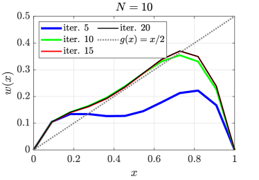
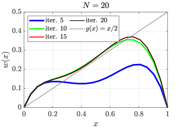
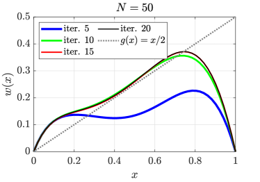
Figure 2: Numerical solutions to the BVP in Section 6.2 with different values of the discretization parameter $N$ and different iterations of the fixed-point computations from Theorem 6.

Figure 2 shows that the fixed-point computations (almost) converge within the first 20 iterations for all the considered values of $N$. In addition, the figure shows that for the 20^th iteration and different values of $N$, the numerical solutions almost coincide, especially for $N=50$ and $N=100$, which further supports the convergence result in Section 6.1.

7 Conclusion

In this paper, we studied a fourth-order boundary value problem with a bounded above and monotonically decreasing right-hand side, showing solution existence and uniqueness for both the original problem and its discrete counterpart obtained through finite difference. We then focused on a particular piecewise linear instance of the right-hand side, showing that the solution to the discrete equation can be obtained through fixed-point iterations and that the solution to the discrete equation converges to the solution of the continuous problem. We illustrated the effectiveness of the fixed-point iterations through a numerical example.

Typical voice production incorporates dynamic VF vibrations and time-varying contact forces (microswitches and beams on elastic foundations also often incorporate dynamic vibrations with contact forces). It would be of interest to extend the techniques covered herein to explore dynamic Euler-Bernoulli beam models with contract forces. Moreover, extensions of the analysis presented herein can be considered in future works to cover more sophisticated beam (e.g., Timoshenko model [45]) and plate models.

References

• [1] B. H. Story and I. R. Titze, “Voice simulation with a body-cover model of the vocal folds,” The Journal of the Acoustical Society of America, vol. 97, no. 2, pp. 1249–1260, 1995.
• [2] M. A. Serry, C. E. Stepp, and S. D. Peterson, “Physics of phonation offset: Towards understanding relative fundamental frequency observations,” The Journal of the Acoustical Society of America, vol. 149, no. 5, pp. 3654–3664, 2021.
• [3] G. E. Galindo, S. D. Peterson, B. D. Erath, C. Castro, R. E. Hillman, and M. Zañartu, “Modeling the pathophysiology of phonotraumatic vocal hyperfunction with a triangular glottal model of the vocal folds,” Journal of Speech, Language, and Hearing Research, vol. 60, no. 9, pp. 2452–2471, 2017.
• [4] M. Zañartu, G. E. Galindo, B. D. Erath, S. D. Peterson, G. R. Wodicka, and R. E. Hillman, “Modeling the effects of a posterior glottal opening on vocal fold dynamics with implications for vocal hyperfunction,” The Journal of the Acoustical Society of America, vol. 136, no. 6, pp. 3262–3271, 2014.
• [5] P. H. Dejonckere and M. Kob, “Pathogenesis of vocal fold nodules: new insights from a modelling approach,” Folia Phoniatrica et Logopaedica, vol. 61, no. 3, pp. 171–179, 2009.
• [6] M. Serry, G. Alzamendi, M. Zanartu, and S. Peterson, “An euler-bernoulli-type beam model of the vocal folds for describing curved and incomplete glottal closure patterns,” arXiv preprint, 2023.
• [7] B. D. Jensen, K. Huang, L. L.-W. Chow, and K. Kurabayashi, “Adhesion effects on contact opening dynamics in micromachined switches,” Journal of Applied Physics, vol. 97, no. 10, p. 103535, 2005.
• [8] B. McCarthy, G. G. Adams, N. E. McGruer, and D. Potter, “A dynamic model, including contact bounce, of an electrostatically actuated microswitch,” Journal of microelectromechanical systems, vol. 11, no. 3, pp. 276–283, 2002.
• [9] M. Hetényi and M. I. Hetbenyi, Beams on elastic foundation: theory with applications in the fields of civil and mechanical engineering, vol. 16. University of Michigan press Ann Arbor, MI, 1946.
• [10] J. Barber, Beams on Elastic Foundations, pp. 353–384. Dordrecht: Springer Netherlands, 2011.
• [11] C. G. Vallabhan and Y. Das, “A refined model for beams on elastic foundations,” International Journal of Solids and Structures, vol. 27, no. 5, pp. 629–637, 1991.
• [12] G. Jones, Analysis of beams on elastic foundations: using finite difference theory. Thomas Telford, 1997.
• [13] R. A. Usmani and M. J. Marsden, “Convergence of a numerical procedure for the solution of a fourth order boundary value problem,” Proceedings of the Indian Academy of Sciences-Section A. Part 3, Mathematical Sciences, vol. 88, no. 1, pp. 21–30, 1979.
• [14] Y. S. Yang, “Fourth-order two-point boundary value problems,” Proceedings of the American Mathematical Society, vol. 104, no. 1, pp. 175–180, 1988.
• [15] A. Aftabizadeh, “Existence and uniqueness theorems for fourth-order boundary value problems,” Journal of Mathematical Analysis and Applications, vol. 116, no. 2, pp. 415–426, 1986.
• [16] Y. Li and H. Yang, “An existence and uniqueness result for a bending beam equation without growth restriction,” in Abstract and Applied Analysis, vol. 2010, Hindawi, 2010.
• [17] Y. Li and Y. Gao, “Existence and uniqueness results for the bending elastic beam equations,” Applied Mathematics Letters, vol. 95, pp. 72–77, 2019.
• [18] Y. Li and Q. Liang, “Existence results for a fully fourth-order boundary value problem,” Journal of Function Spaces and Applications, vol. 2013, 2013.
• [19] D. Quang A and N. T. K. Quy, “New fixed point approach for a fully nonlinear fourth order boundary value problem,” Boletim da Sociedade Paranaense de Matematica, vol. 36, no. 4, pp. 209–223, 2018.
• [20] R. P. Agarwal, “On fourth order boundary value problems arising in beam analysis,” Differential and Integral Equations, vol. 2, no. 1, pp. 91–110, 1989.
• [21] Z. Bai, “The method of lower and upper solutions for a bending of an elastic beam equation,” Journal of Mathematical Analysis and Applications, vol. 248, no. 1, pp. 195–202, 2000.
• [22] G. Han and F. Li, “Multiple solutions of some fourth-order boundary value problems,” Nonlinear Analysis: Theory, Methods & Applications, vol. 66, no. 11, pp. 2591–2603, 2007.
• [23] H. Feng, D. Ji, and W. Ge, “Existence and uniqueness of solutions for a fourth-order boundary value problem,” Nonlinear Analysis: Theory, Methods & Applications, vol. 70, no. 10, pp. 3561–3566, 2009.
• [24] Y. Li and X. Chen, “Solvability for fully cantilever beam equations with superlinear nonlinearities,” Boundary Value Problems, vol. 2019, no. 1, pp. 1–9, 2019.
• [25] D. Quang A and N. T. Huong, “Existence results and numerical method for a fourth order nonlinear problem,” International Journal of Applied and Computational Mathematics, vol. 4, no. 6, p. 148, 2018.
• [26] D. Quang A and T. K. Quy, “Existence results and iterative method for solving the cantilever beam equation with fully nonlinear term,” Nonlinear Analysis: Real World Applications, vol. 36, pp. 56–68, 2017.
• [27] J. Caballero, J. Harjani, and K. Sadarangani, “Uniqueness of positive solutions for a class of fourth-order boundary value problems,” in Abstract and Applied Analysis, vol. 2011, Hindawi, 2011.
• [28] M. Ruyun, Z. Jihui, and F. Shengmao, “The method of lower and upper solutions for fourth-order two-point boundary value problems,” Journal of Mathematical Analysis and Applications, vol. 215, no. 2, pp. 415–422, 1997.
• [29] H. L. Royden and P. Fitzpatrick, Real analysis, vol. 32. Macmillan New York, 1988.
• [30] T. Tao, An introduction to measure theory, vol. 126. American Mathematical Soc., 2011.
• [31] E. Zeidler, Applied functional analysis: applications to mathematical physics, vol. 108. Springer Science & Business Media, 2012.
• [32] R. A. Usmani and M. J. Marsden, “Numerical solution of some ordinary differential equations occurring in plate deflection theory,” Journal of Engineering Mathematics, vol. 9, no. 1, pp. 1–10, 1975.
• [33] A.-M. Wazwaz, “The numerical solution of special fourth-order boundary value problems by the modified decomposition method,” International journal of computer mathematics, vol. 79, no. 3, pp. 345–356, 2002.
• [34] A. Ali, “Numerical solution of fourth order boundary-value problems using haar wavelets,” Appl. Math. Sci., vol. 5, no. 63, pp. 3131–3146, 2011.
• [35] W. K. Zahra, “Finite-difference technique based on exponential splines for the solution of obstacle problems,” International Journal of Computer Mathematics, vol. 88, no. 14, pp. 3046–3060, 2011.
• [36] V. S. Ertürk and S. Momani, “Comparing numerical methods for solving fourth-order boundary value problems,” Applied Mathematics and Computation, vol. 188, no. 2, pp. 1963–1968, 2007.
• [37] M. A. Hajji and K. Al-Khaled, “Numerical methods for nonlinear fourth-order boundary value problems with applications,” International Journal of Computer Mathematics, vol. 85, no. 1, pp. 83–104, 2008.
• [38] O. Mangasarian and R. Meyer, “Absolute value equations,” Linear Algebra and Its Applications, vol. 419, no. 2-3, pp. 359–367, 2006.
• [39] F. Mezzadri, “On the solution of general absolute value equations,” Applied mathematics letters, vol. 107, p. 106462, 2020.
• [40] J. Rohn, V. Hooshyarbakhsh, and R. Farhadsefat, “An iterative method for solving absolute value equations and sufficient conditions for unique solvability,” Optimization Letters, vol. 8, pp. 35–44, 2014.
• [41] S.-L. Wu and C.-X. Li, “The unique solution of the absolute value equations,” Applied Mathematics Letters, vol. 76, pp. 195–200, 2018.
• [42] S.-L. Wu and C.-X. Li, “A note on unique solvability of the absolute value equation,” Optimization Letters, vol. 14, no. 7, pp. 1957–1960, 2020.
• [43] M. Radons and S. M. Rump, “Convergence results for some piecewise linear solvers,” Optimization Letters, vol. 16, no. 6, pp. 1663–1673, 2022.
• [44] R. A. Horn and C. R. Johnson, Matrix analysis. Cambridge university press, 2 ed., 2013.
• [45] P. S. Timoshenko, “Lxvi. on the correction for shear of the differential equation for transverse vibrations of prismatic bars,” The London, Edinburgh, and Dublin Philosophical Magazine and Journal of Science, vol. 41, no. 245, pp. 744–746, 1921.