Theoretical determination of Ising-type transition by using the Self-Consistent Harmonic Approximation

Abstract

Over the years, the Self-Consistent Harmonic Approximation (SCHA) has been successfully utilized to determine the transition temperature of many different magnetic models, particularly the Berezinskii-Thouless-Kosterlitz transition in two-dimensional ferromagnets. More recently, the SCHA has found application in describing ferromagnetic samples in spintronic experiments. In such a case, the SCHA has proven to be an efficient formalism for representing the coherent state in the ferromagnetic resonance state. One of the main advantages of using the SCHA is the quadratic Hamiltonian, which incorporates thermal spin fluctuations through renormalization parameters, keeping the description simple while providing excellent agreement with experimental data. In this article, we investigate the SCHA application in easy-axis magnetic models, a subject that has not been adequately explored to date. We obtain both semiclassical and quantum approaches of the SCHA for a general anisotropic magnetic model and employ them to determine various quantities such as the transition temperature, spin-wave energy spectrum, magnetization, and critical exponents. To verify the accuracy of the method, we compare the SCHA results with experimental and Monte Carlo simulation data for many distinct well-known magnetic materials.

I Introduction and motivation

The continuous advancements in material science have driven the device miniaturization to sizes approaching the atomic scale. In this scale, dimensionality plays a crucial role and, usually, the three-dimensional Physics of macroscopic models does not apply as one might expect. An example of this is the Berezinskii-Thouless-Kosterlitz (BKT) transition, defined by a topological phase transition exclusively of two-dimensional models with order parameters exhibiting continuous $O(2)$ symmetry, typically found in magnetic models with easy-plane anisotropy. The BKT transition was initially confirmed in the superfluid state of thin Helium filmsprl40.1727, as well as in controlled experiments involving ultracold trapping of 2D Bose gasnature441.7097. Although the theoretical analysis of BKT transition has been performed in magnetic models over the years, obtaining experimental results has been challenging due to the difficulty of finding genuine two-dimensional magnetic materials with planar anisotropy. In many cases, the systems studied are quasi-two-dimensional magnets composed of weakly coupled layers. It is only recently that the synthesis of two-dimensional magnetic compounds, such as those based on rare-earth oxide YbMgGaO${}_{4}$prx10.011007; natcommun10.4530, has made it possible to observe the occurrence of the BKT transition in magnetic modelsnatcommun11.1.

Contrary to the easy-plane scenario, we have the 2D magnetic models with easy-axis anisotropy, which break the continuous internal symmetry and provide an Ising-type transition. It should be noted that in this case, the Mermin-Wagner theorem does not apply, and even a minor anisotropy is sufficient to induce a finite transition temperature prb38.12015; prb59.6229; prb62.3771. In addition, since the first synthesis of graphene monolayersscince306.5696, there has been tremendous interest in utilizing low-dimensional materials for technological applications. Specifically, numerous studies focused on the deployment of spintronic devices, which employ spin rather than electronic charge for processing and storing informationnpj2d4.17; natnano15.545. However, graphene is a strongly diamagnetic material and shows a weak spin-orbit couplingrmp92.021003, which hinders its effectiveness as a spin current detector via Inverse Spin-Hall Effectapl88.182509. On the other hand, the recent development of the 2D van der Waals magnetsnature546.265; nature563.47; apl8.031305 has further intensified research in low-dimensional magnets. For instance, Torelli et al. used Monte Carlo simulation models to investigate the role of anisotropy in several two-dimensional magnets2dmater4.045018, some of which exhibit order even at room temperature.

As it is well-known, there is no theoretical method capable of yielding exact results in two-dimensional magnetic models, and approximations are required to extract any physical information about the system. Among the most traditional methods, we have bosonic representations such as the Holstein-Primakoff (HP), Schwinger, and Dyson-Maleev formalism, which replace the spin by magnon annihilation/creation operators (for a review of bosonic representations, and other methods, see Ref. auerbach; pires. Each method is more or less convenient depending on the magnetic system properties, but in the simpler description of non-interacting spin waves, they all result in quadratic models. However, eventually, the traditional quadratic representation is not suficient to describe the properties even as an initial approximation. In the spin conductivity evaluation, for example, the first non-null contributions arise from terms associated with interacting magnonsprb75.214403. These contributions necessitate the inclusion of terms beyond the second order in the Hamiltonian. In these scenarios, an extensive perturbative analysis is required, and the solution can be hard to be obtained. Therefore, the SCHA formalism emerges as an alternative to the traditional bosonic representations in order to address these complexities.

The main idea of the SCHA is the replacement of the original spin Hamiltonian by another one containing only quadratic terms, similar to the aforementioned methods, involving the canonically conjugate fields (operators, in the quantum approach) $\varphi$ and $S^{z}$. However, unlike the Holstein-Primakoff formalism, the SCHA includes spin fluctuations through self-consistently solved renormalization parameters. Therefore, the SCHA model is simultaneously simple and precise in determining the thermodynamics of ordered phases in magnetic materials. Indeed, over the years, the SCHA has been successfully used to determine the critical temperature prb49.9663; pla202.309; prb51.16413; prb54.3019; ssc104.771; prb59.6229, the topological BKT transition pla166.330; prb48.12698; prb49.9663; prb50.9592; ssc100.791; prb53.235; prb54.3019; prb54.6081; ssc112.705; epjb2.169; pssb.242.2138; prb78.212408; jmmm452.315, and the large-D quantum phase transition pasma373.387; jpcm20.015208; pasma388.21; pasma388.3779; jmmm357.45 in a wide variety of magnetic models. In addition, the description by using canonically conjugate fields supply the most convenient formalism to describe coherent states in magnetism, as demonstrated by Moura and Lopesjmmm472.1. More recently, Moura has applied the same formalism to present a detailed theoretical analysis of the ferromagnetic resonance and spin pumping process at the ferromagnetic/normal metal junctionprb106.054313.

In this paper, we employ the SCHA to analyze ferro and antiferromagnetic 2D models exhibiting easy-axis anisotropy. While the method has been extensively utilized to investigate magnetic models with easy-plane anisotropy, we have a dearth of studies focusing on the effects of easy-axis anisotropy. Therefore, we developed the SCHA formalism for determining the properties of anisotropic two-dimensional magnetic models, which are given by the Hamiltonian

$$H=\pm J\sum_{\langle i,j\rangle}(S_{i}^{y}S_{j}^{y}+S_{i}^{z}S_{j}^{z}+\lambda_{0}S_{i}^{x}S_{j}^{x})-g\mu_{B}\sum_{i}{\bf S_{i}}\cdot{\bf B_{i}},$$ (1)

where $-J$ ($+J$) represents the ferromagnetic (antiferromagnetic) coupling, $\lambda_{0}$ is the (bare) anisotropic constant, and the first sum is carried out over nearest-neighbor sites. The last term is the Zeeman energy associated with the magnetic field ${\bf B}$. For a thin film, we can write ${\bf B}=\mu_{0}({\bf H_{\textrm{ext}}}-N_{x}{\bf M_{x}})$, where ${\bf H_{\textrm{ext}}}$ is the external $H$-field and $-N_{x}{\bf M_{x}}$ is the demagnetizing field. Here, we are considering the special case with uniform magnetization along the x-axis that provides the demagnetization factors $N_{x}=1$, while $N_{y}=N_{z}=0$. In the antiferromagnetic case, ${\bf M}={\bf 0}$, and there is no demagnetizing field to be considered. For ferromagnetic models, the demagnetizing field effects are considered replacing $\lambda_{0}$ by an effective anisotropy, as demonstrated in the next section. To facilitate the application of the SCHA formalism, we consider sites located on the yz-plane while the anisotropy is defined along the x-axis. The easy-axis anisotropy is achieved by setting $\lambda>1$, and the limit $\lambda$ approaching infinity corresponds to the Ising model. Alternatively, a uniaxial anisotropy, which also represents easy-axis anisotropic systems, could be considered in replacement of $\lambda S_{i}^{x}S_{j}^{x}$ with minor modifications. Moreover, other interactions or anisotropies can be easily implemented, enabling the application of formalism in a wide variety of situations. The SCHA proves to be a valuable tool for determining essential properties of the ordered phase, such as the spectrum energy, the transition temperature, the magnetization, and others. The results obtained from SCHA exhibit excellent agreement with numerous experimental and Monte Carlo simulation studies.

II The SCHA formalism

As mentioned earlier, the initial step of the SCHA formalism is replacing the spin fields with quadratic representations of angle $\varphi$ around the z-axis and its conjugate momentum, denoted as $S^{z}$. Typically, in problems covering planar anisotropy, we consider spins located on the xy-plane and define the quantization along the z-axis. However, this choice is not mandatory. In the present context, to properly apply the SCHA formalism, we opt to place the spins on the yz-plane, while retaining the x-axis as the magnetization axis, as shown in Fig. (1).

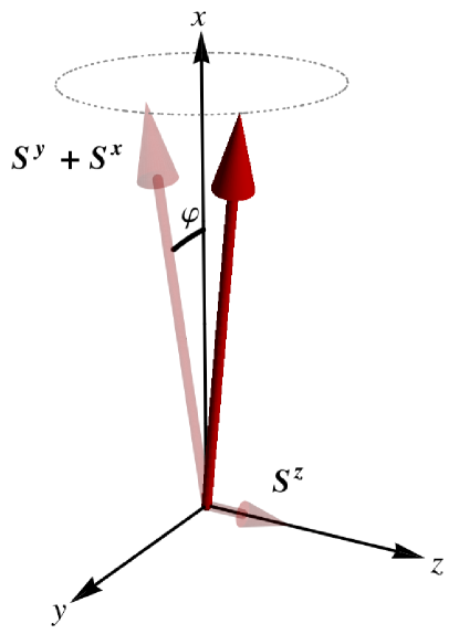
Figure 1: The quantization axis is adopted along the $x$ axis. $S^{z}$ and $\varphi$ are canonically conjugate, and $\varphi$ is defined as the angle between the spin projection on the $xy$ plane and the $x$ axis.

Due to the anisotropy, $\varphi\ll 1$ and thus, the transverse spin components $S^{y}$ and $S^{z}$ are much smaller than the longitudinal component $S^{x}$. From the classical point of view, the fields $\varphi_{i}$ and $S_{j}^{z}$, on sites i and j, respectively, satisfy the Poisson bracket $\{\varphi_{i},S_{j}^{z}\}=\delta_{ij}$, and the quantization is achieved by promoting the fields to operators that obey the commutation relation $[\varphi_{i},S_{j}^{z}]=\delta_{ij}$.

We can consider the spin as a quantum operator from the beginning, and then use the Villain representationjp35.27 to represent the raising operator as $S_{i}^{+}=e^{i\varphi}\sqrt{\tilde{S}^{2}-S_{i}^{z}(S_{i}^{z}+1)}$, where $\tilde{S}=\sqrt{S(S+1)}$. Alternatively, we can start in the semiclassical limit, for which the spins are represented by three-dimensional vectors. Then, we perform the quantization by the usual second quantization procedure. Since the second approach is more convenient for the present scenario, we will proceed with this approach.

Semiclassical approach

To begin with, we write the Hamiltonian (1) in terms of the $\varphi$ and $S^{z}$ fields, which results in rCl H&=J2∑_⟨ij⟩[-(1+λ_0)f_ijcosΔφ+(1-λ_0)f_ijcosΣφ±
±2S_i^z S_j^z]-gμ_B B^x∑_i