Transient spectroscopy from time-dependent electronic-structure theory without multipole expansions

Abstract

Based on the work done by an electromagnetic field on an atomic or molecular electronic system, a general gauge invariant formulation of transient absorption spectroscopy is presented within the semi-classical approximation. Avoiding multipole expansions, a computationally viable expression for the spectral response function is derived from the minimal-coupling Hamiltonian of an electronic system interacting with one or more laser pulses described by a source-free, enveloped electromagnetic vector potential. With a fixed-basis expansion of the electronic wave function, the computational cost of simulations of laser-driven electron dynamics beyond the dipole approximation is the same as simulations adopting the dipole approximation. We illustrate the theory by time-dependent configuration interaction and coupled-cluster simulations of core-level absorption and circular dichroism spectra.

I Introduction

Using technology developed in the past two decades, ultrashort laser pulses with attosecond duration have enabled the observation and manipulation of multi-electron dynamics in atoms, molecules, and materials, thus opening new research avenues in physics and chemistry Corkum and Krausz (2007); Krausz and Ivanov (2009); Nisoli et al. (2017). Quantum-mechanical simulations are mandatory to properly understand, interpret, and predict advanced attosecond experiments. While nuclear motion becomes important on longer time-scales (femtoseconds), one- and multi-electron ionization dynamics constitute major challenges for time-dependent electronic-structure simulations, along with electron-correlation effects Klinker et al. (2018).

Single active electron (SAE) models Kulander (1988); Schafer and Kulander (1990); Kulander et al. (1993) that, at best, only account for electron correlation through an effective potential are widely used to study processes induced by lasers with frequency well below any multi-electron excitation energy. As the frequency increases and approaches resonance with a multi-electron excited state, the SAE approximation breaks down and a correlated many-body method should be applied instead Lezius et al. (2001); Markevitch et al. (2003).

Regardless whether the SAE model or a many-body description is used, most simulations of laser-induced processes employ the electric-dipole approximation where the magnetic component of the laser field is neglected and the electric component is assumed to be spatially uniform. This is an excellent approximation when the spatial extent of the electronic system is small compared with the wavelength of the laser field. Attosecond laser pulses, however, are commonly generated by high harmonic generation in the extreme ultraviolet and X-ray spectral regions where beyond-dipole effects may become non-negligible. It is, therefore, of interest to include higher-order electric and magnetic multipole interactions in simulations of laser-driven electron dynamics, preferably without incurring a significant computational penalty.

Within response theory Olsen and Jørgensen (1985), which is essentially time-dependent perturbation theory Fourier-transformed to the frequency domain, beyond-dipole effects have been studied using the full plane-wave vector potential for the semiclassical description of the matter-field interaction List et al. (2015, 2017); Sørensen et al. (2019); van Horn et al. (2022). Due to the use of perturbation theory and the neglect of terms quadratic in the vector potential, these studies are limited to weak laser fields but do not suffer from issues such as origin-dependence and slow basis-set convergence that may arise from the use of multipole expansions Bernadotte et al. (2012); Lestrange et al. (2015); Sørensen et al. (2017a); van Horn et al. (2023). Conceptually, at least, it is rather straightforward to generalize the response-theory approaches to the time domain, avoiding perturbation theory altogether and hence enabling the study of both weak- and strong-field processes without multipole expansions.

The theory of transient absorption spectroscopy (TAS), see, e.g., recent work by Wu et al. (2016), has been formulated in the framework of the electric-dipole approximation. In the present work, we present a generalization that accounts for the presence of spatially non-uniform fields, which reduces to the original formulation in the long-wavelength (electric-dipole) limit. In line with the previous work based on response theory List et al. (2015, 2017); Sørensen et al. (2019); van Horn et al. (2022), we present initial test simulations on small molecules in the weak-field limit using time-dependent configuration-interaction (TDCI) Rohringer et al. (2006); Krause et al. (2007); Schlegel et al. (2007); Pabst et al. (2011); White et al. (2016) and time-dependent coupled-cluster (TDCC) Ofstad et al. (2023) theories. Ignoring ionization processes, we use static, atom-centered Gaussian basis sets such that the prerequisite integrals involving the full plane-wave vector potential can be computed using the recent implementation reported by Sørensen et al. (2019). This allows us to validate our implementation of the generalized theory of TAS by comparing with previously reported theoretical pump-probe and X-ray absorption spectra. In addition, we compute the anisotropic X-ray circular dichroism (CD) spectrum of hydrogen peroxide generated from simulations of the electrons interacting with circularly polarized laser pulses Kfir et al. (2015); Bandrauk and Yuan (2016); Shao et al. (2020); Ma et al. (2016); Zhong et al. (2021); Chen et al. (2016), comparing with the CD spectrum predicted by the rotatory strength tensor Pedersen and Hansen (1995).

II Theory

Atomic and molecular transient (as well as steady-state) absorption spectra can be obtained by computing the spectral response function $S(\omega)$ which, in turn, is obtained from a frequency-resolved analysis of the total energy transfer $\Delta\mathcal{E}$ between an electromagnetic field and the electronic system. The spectral response function $S(\omega)$ is defined such that it satisfies the relation

$$\Delta\mathcal{E}=\int_{0}^{\infty}\mathrm{d}\omega\ \omega S(\omega).$$ (1)

The absorption cross section $\sigma(\omega)$ can be computed as

$$\sigma(\omega)=\frac{\omega S(\omega)}{I(\omega)},$$ (2)

where $I(\omega)$ is the total field energy per unit area at frequency $\omega$. In this work, however, we shall focus on the spectral response function. We first formulate a general, gauge invariant theory for the energy transfer, proceeding to the derivation of the spectral response function for the specific case of an enveloped, source-free electromagnetic field without multipole expansion.

II.1 Energy transfer

We consider an atomic or molecular electronic system exposed to the classical electromagnetic fields

$$\bm{E}(\bm{r},t)=-\partial_{t}\bm{A}(\bm{r},t)-\nabla\phi(\bm{r},t),$$ (3)

$$\bm{B}(\bm{r},t)=\nabla\times\bm{A}(\bm{r},t),$$ (4)

where $\bm{A}(\bm{r},t)$ and $\phi(\bm{r},t)$ are the vector and scalar potentials, respectively. Specifically, we will consider the interactions of the electrons with laser pulses, i.e., the physical electric and magnetic fields, $\bm{E}$ and $\bm{B}$, are nonzero only in a finite time interval and vanish as $t\to\pm\infty$. Within the nonrelativistic, clamped-nuclei Born-Oppenheimer approximation the time evolution of the electronic system is governed by the electronic Schrödinger equation

$$\mathrm{i}\ket{\dot{\Psi}(t)}=H(t)\ket{\Psi(t)},\qquad\ket{\Psi(t\to-\infty)}=\ket{\Psi_{0}},$$ (5)

where $\ket{\Psi_{0}}$ is the initial wave function of the electrons, typically the ground-state wave function in the absence of external fields. The semiclassical, minimal-coupling Hamiltonian is given by

$$H(t)=\frac{1}{2}\pi^{2}(\bm{r},t)+W-\phi(\bm{r},t),$$ (6)

where $\bm{\pi}(\bm{r},t)=\bm{p}+\bm{A}(\bm{r},t)$ is the kinetic momentum operator and $W$ represents all Coulomb interactions among the electrons and (clamped) nuclei. Throughout this paper, summation over electrons will be implicitly assumed for brevity of notation, and Hartree atomic units are used. We have also skipped the spin-Zeeman term as we will use only closed-shell, spin-restricted wave functions in the present work.

We wish to derive a general expression for the spectral response function $S(\omega)$ in Eq. (1). Physically, the total energy transfer $\Delta\mathcal{E}$ expresses the work performed on the electronic system by the external electromagnetic fields, and the rate of change of the energy is referred to as the power. In classical electrodynamics Jackson (1975), the power function of an electron in an electromagnetic field is given by $P=-\bm{E}\cdot\bm{v}$, where $\bm{v}$ is the velocity of the electron. This is also the energy lost by the electromagnetic field as calculated by Poynting’s theorem Jackson (1975), ensuring energy conservation (of the particle and field systems together). The quantum-mechanical power operator can be obtained by Weyl quantization Weyl (1927) as

$$P(\bm{r},t)=-\frac{1}{2}\left(\bm{E}(\bm{r},t)\cdot\bm{\pi}(\bm{r},t)+\bm{\pi}(\bm{r},t)\cdot\bm{E}(\bm{r},t)\right).$$ (7)

Hence, we may express the total energy transferred from the field to the electronic system as

$$\Delta\mathcal{E}=\int_{-\infty}^{\infty}\mathrm{d}t\ \braket{P(\bm{r},t)}.$$ (8)

In previous work on transient absorption spectroscopy—see, e.g., Refs. Tannor (2007); Wu et al. (2016); Skeidsvoll et al. (2020); Guandalini et al. (2021)—the energy transfer is expressed as the integral

$$\Delta\mathcal{E}=\int_{-\infty}^{\infty}\mathrm{d}t\ \frac{\mathrm{d}\mathcal{E}(t)}{\mathrm{d}t},$$ (9)

where $\mathcal{E}(t)$ is the instantaneous energy of the electrons. At this point, the instantaneous energy is typically equated with the quantum-mechanical expectation value of the Hamiltonian, $\braket{H(t)}=\braket{\Psi(t)}{H(t)}{\Psi(t)}$. In general, however, neither the expectation value $\braket{H(t)}$ nor the Hamilton function in classical mechanics Goldstein (1980) equals the energy of the electrons when a time-dependent external electromagnetic field is present. This is clear from the fact that both $\braket{H(t)}$ and $\mathrm{d}\braket{H(t)}/\mathrm{d}t$ are gauge-dependent quantities. Instead, the operator Yang (1976a); Kobe and Yang (1987)

$$K(t)=H(t)+\phi(\bm{r},t)=\frac{1}{2}\pi^{2}(\bm{r},t)+W,$$ (10)

can be regarded as a (generally time-dependent) energy operator which yields gauge invariant expansion coefficients and transition probabilities when the wave function is expanded in its (generally time-dependent) eigenstates. Using the energy operator, Eq. (10), and the Ehrenfest theorem, we find

$$\frac{\mathrm{d}\mathcal{E}(t)}{\mathrm{d}t}=\frac{\mathrm{d}\braket{K(t)}}{\mathrm{d}t}=\braket{P(\bm{r},t)},$$ (11)

which leads to Eq. (8) upon substitution in Eq. (9). We refer to references Yang (1976a, b); Kobe and Smirl (1978); Kobe (1978); Kobe and Yang (1980); Aharonov and Au (1981); Kobe and Wen (1982); Kobe and Yang (1987) for further discussions of the intricacies of gauge invariance in external time-varying fields.

Within the electric-dipole approximation, $\bm{A}(\bm{r},t)\approx\bm{A}(\bm{0},t)=\bm{A}(t),\quad\phi(\bm{r},t)=0$, which was assumed in previous work Tannor (2007); Wu et al. (2016); Skeidsvoll et al. (2020); Guandalini et al. (2021), the power operator becomes $P(t)=-\bm{\pi}(t)\cdot\bm{E}(t)$. Inserting this expression into Eq. (8) yields

$$\Delta\mathcal{E}=-\int_{-\infty}^{\infty}\mathrm{d}t\ \braket{\bm{\pi}(t)}\cdot\bm{E}(t).$$ (12)

Using the Ehrenfest theorem,

$$\frac{\mathrm{d}\braket{\bm{r}}}{\mathrm{d}t}=\braket{\bm{\pi}(t)},$$ (13)

and integration by parts, we arrive at

$$\Delta\mathcal{E}=\int_{-\infty}^{\infty}\mathrm{d}t\ \braket{\bm{r}}\cdot\dot{\bm{E}}(t),$$ (14)

which agrees with the expressions obtained in Refs. Tannor (2007); Wu et al. (2016); Skeidsvoll et al. (2020); Guandalini et al. (2021).

Identifying the instantaneous energy as the expectation value $\braket{H(t)}$ is valid when the scalar potential vanishes which, in turn, is a valid choice with the Coulomb gauge condition $\nabla\cdot\bm{A}(\bm{r},t)=0$ whenever the electric field is divergence-free (no charge contributions to the electric field), i.e. within radiation gauge Schlicher et al. (1984). It is a peculiarity of the electric-dipole approximation that the correct energy transfer is obtained from $\braket{H(t)}$ with the choices $\bm{A}(\bm{r},t)=\bm{0}$ and $\phi(\bm{r},t)=-\bm{r}\cdot\bm{E}(t)$.

II.2 Representation of laser pulses without multipole expansion

From here on we will assume a divergence-free electric field and work in the radiation gauge such that $K(t)=H(t)$. Following common practice, we separate the Hamiltonian into a time-independent and a time-dependent part,

$$H(t)=H_{0}+V(t),$$ (15)

$$H_{0}=\frac{1}{2}p^{2}+W,$$ (16)

$$V(t)=\bm{A}(\bm{r},t)\cdot\bm{p}+\frac{1}{2}A^{2}(\bm{r},t).$$ (17)

In the context of time-dependent perturbation theory or frequency-dependent response theory, the weak-field approximation—i.e., neglecting the term quadratic in the vector potential—is usually invoked, although it is not formally necessary to do so List et al. (2015, 2017); Sørensen et al. (2019); van Horn et al. (2022). For the real-time simulations pursued in the present work, invoking the weak-field approximation does not lead to any simplifications and, hence, we retain the quadratic term in all simulations.

The vector potential that solves the Maxwell equations within the Coulomb gauge is a linear combination of plane waves. However, this is impractical for modelling ultra-fast laser pulses. We will instead model the vector potential as a linear combination of enveloped plane waves

$$\bm{A}(\bm{r},t)=\sum_{m}\bm{A}_{m}(\bm{r},t)G_{m}(t)$$

$$=\sum_{m}A_{m}\mathrm{Re}\{\bm{u}_{m}\mathrm{e}^{\mathrm{i}(\bm{k}_{m}\cdot\bm{r}-\omega_{m}t-\gamma_{m})}\}G_{m}(t),$$ (18)

where each term in the sum models a single pulse with amplitude $A_{m}$, carrier frequency $\omega_{m}$, and carrier-envelope phase $\gamma_{m}$. The Coulomb gauge condition implies that the (complex) polarization vector $\bm{u}_{m}$ is orthogonal to the real wave vector $\bm{k}_{m}$, which has length $\omega_{m}/c$ where $c$ is the speed of light. The electric- and magnetic-field amplitudes of each pulse are $E_{m}=\omega_{m}A_{m}$ and $B_{m}=E_{m}/c$, respectively, and we define the peak intensity of each pulse to be

$$I_{m}=\frac{1}{2}\epsilon_{0}cE_{m}^{2}.$$ (19)

Chirped laser pulses can be modelled by letting $\gamma_{m}$ be time-dependent.

In experimental work, Gaussian functions are often favored for the envelopes $G_{m}(t)$. In numerical studies, however, Gaussians are inconvenient due to their long tails and infinite support. For this reason, we use trigonometric envelopes on the form Barth and Lasser (2009)

$$G_{m}(t)=\begin{cases}\cos^{n}{\left(\frac{\pi(t-t_{m})}{T_{mn}}\right)}&|t-t_{m}|\leq\frac{T_{mn}}{2}\\ 0&|t-t_{m}|>\frac{T_{mn}}{2}\end{cases}$$ (20)

where $n>0$ is a chosen parameter, $t_{m}$ is the central time of pulse $m$, and $T_{mn}$ is the total duration of $\bm{A}_{m}$. The total duration depends on $n$ and may be computed from

$$T_{mn}=\frac{\pi\tau_{m}}{2\arccos(2^{-1/(2n)})},$$ (21)

where $\tau_{m}$ is the full width at half maximum of $G^{2}_{m}(t)$, i.e., $\tau_{m}$ is approximately the desired experimental pulse duration defined from the intensity distribution Barth and Lasser (2009).

The trigonometric envelopes, Eq. (20), define a sequence of functions that rapidly and uniformly converges to the Gaussian function $\exp(-2\ln{(2)}(t-t_{m})^{2}/\tau_{m}^{2})$ for increasing values of $n$ Barth and Lasser (2009). Moreover, in contrast to finite numerical representations of Gaussian envelopes, the trigonometric envelopes guarantee that the dc (zero-frequency) component of the electric field vanishes identically for any choice of $n>0$, in agreement with the far-field approximation of the Maxwell equations Rauch and Mourou (2006).

A similar setup has been used before in grid treatments of single-electron systems Førre et al. (2005, 2006); Moe and Førre (2018) where pulses on the form

$$\bm{A}(\bm{r},t)=A_{0}\sin^{2}{\left(\frac{\pi(\omega t-\bm{k}\cdot\bm{r})}{\omega T}\right)}\sin{\left(\omega t-\bm{k}\cdot\bm{r}\right)}\bm{u},$$ (22)

were used. Here, $\bm{u}$ is a real polarization vector and the envelope depends both on time and on spatial coordinates. This has the benefit of modelling the overall shape of the pulse in space, albeit with potential edge effects if the approximation $\bm{A}(\bm{r},t)\approx 0$ at $t=0$ and $t=T$ is made along with a neglect of the spatial non-periodicity. The pulse with the purely time-dependent envelope, Eq. (20) with $n=2$, may be regained from the spatio-temporal envelope by an expansion through lowest order in $\bm{k}\cdot\bm{r}/n_{cyc}$, where $n_{cyc}$ is the number of optical cycles of the pulse.

II.3 The spectral response function

Since we have assumed a divergence-free electric field, the power operator becomes $P(\bm{r},t)=-\bm{E}(\bm{r},t)\cdot\bm{\pi}(\bm{r},t)$, and Eq. (8) simplifies to

$$\Delta\mathcal{E}=-\int_{-\infty}^{\infty}\mathrm{d}t\ \langle\bm{E}(\bm{r},t)\cdot\bm{\pi}(\bm{r},t)\rangle.$$ (23)

Using the Fourier transform convention

$$f(t)=\mathcal{F}_{\omega}\bigl{[}\tilde{f}(\omega)\bigr{]}=\frac{1}{\sqrt{2\pi}}\int_{-\infty}^{\infty}\mathrm{d}\omega\ \tilde{f}(\omega)e^{\mathrm{i}\omega t},$$ (24)

$$\tilde{f}(\omega)=\mathcal{F}_{t}\bigl{[}f(t)\bigr{]}=\frac{1}{\sqrt{2\pi}}\int_{-\infty}^{\infty}\mathrm{d}t\ f(t)e^{-\mathrm{i}\omega t},$$ (25)

the integration over time in Eq. (23) can be turned into an integration over frequency,

$$\Delta\mathcal{E}=\int_{-\infty}^{\infty}\mathrm{d}\omega\ Y(\omega),$$ (26)

with

$$Y(\omega)=-\mathcal{F}_{t}\left[\mathrm{i}\omega\langle\tilde{\bm{A}}(\bm{r},\omega)^{*}\cdot\bm{\pi}(\bm{r},t)\rangle\right],$$ (27)

where we have used $\tilde{\bm{E}}(\bm{r},\omega)^{*}=\mathrm{i}\omega\tilde{\bm{A}}(\bm{r},\omega)^{*}$.

Introducing

$$f_{1,m}(\bm{r})=\cos{(\bm{k}_{m}\cdot\bm{r})},$$ (28)

$$f_{2,m}(\bm{r})=\sin{(\bm{k}_{m}\cdot\bm{r})},$$ (29)

$$g_{1,m}(t)=\cos{(\omega_{m}t+\gamma_{m})}G_{m}(t),$$ (30)

$$g_{2,m}(t)=\sin{(\omega_{m}t+\gamma_{m})}G_{m}(t),$$ (31)

$$\bm{u}_{m}^{ij}=\delta_{ij}\mathrm{Re}(\bm{u}_{m})+\epsilon_{ij}\mathrm{Im}(\bm{u}_{m}),$$ (32)

where $\delta_{ij}$ is the Kronecker delta and $\epsilon_{ij}$ is the Levi-Civita symbol, the vector potential, Eq. (II.2), can be recast as

$$\bm{A}_{m}(\bm{r},t)G_{m}(t)=A_{m}\sum_{i,j=1}^{2}\bm{u}_{m}^{ij}f_{i,m}(\bm{r})g_{j,m}(t).$$ (33)

Equation (27) can now be written as

$$Y(\omega)=\omega\sum_{m}\sum_{i,j=1}^{2}\tilde{F}_{ij,m}(\omega)\tilde{g}_{j,m}(-\omega),$$ (34)

where $\tilde{F}_{ij,m}(\omega)$ is the Fourier transform of the function

$$F_{ij,m}(t)=-\mathrm{i}A_{m}\bm{u}_{m}^{ij}\cdot\Biggl{[}\langle f_{i,m}(\bm{r})\bm{p}\rangle\Biggr{.}$$

$$\left.+\sum_{n}\sum_{k,l=1}^{2}A_{n}\bm{u}_{n}^{kl}\langle f_{k,n}(\bm{r})f_{i,m}(\bm{r})\rangle g_{l,n}(t)\right].$$ (35)

Hence,

$$\Delta\mathcal{E}=\int_{0}^{\infty}\mathrm{d}\omega\ \omega\sum_{m}\sum_{i,j=1}^{2}\left[(1-\mathcal{P})\tilde{F}_{ij,m}(\omega)\tilde{g}_{j,m}(-\omega)\right],$$ (36)

where $\mathcal{P}$ is the parity operator defined by $\mathcal{P}f(\omega)=f(-\omega)$. The spectral response function thus becomes

$$S(\omega)=\sum_{m}\sum_{ij=1}^{2}(1-\mathcal{P})\tilde{F}_{ij,m}(\omega)\tilde{g}_{j,m}(-\omega),$$ (37)

which can be computed by sampling $F_{ij,m}(t)$ during a simulation, followed by Fourier transformation in a post-processing step.

In the electric-dipole approximation, $f_{1,m}(\bm{r})=1$ and $f_{2,m}(\bm{r})=0$, and in this case the spectral response function reduces to

$$S(\omega)=2\mathrm{Im}\left[\langle\tilde{\bm{\pi}}\rangle(\omega)\cdot\tilde{\bm{A}}(\omega)^{*}\right],$$ (38)

or, equivalently,

$$S(\omega)=-2\mathrm{Im}\left[\langle\tilde{\bm{d}}\rangle(\omega)\cdot\tilde{\bm{E}}(\omega)^{*}\right],$$ (39)

in terms of the dipole operator $\bm{d}=-\bm{r}$. The latter expression, Eq. (39), was used in Refs. Tannor (2007); Wu et al. (2016); Skeidsvoll et al. (2020); Guandalini et al. (2021). We remark that Eqs. (38) and (39) are equivalent only if the Ehrenfest theorem, Eq. (13), is satisfied, i.e., for fully variational many-body wave function approximations, and in the limit of complete one-electron basis set.

For the visual presentation of spectra we use normalized spectral response functions

$$\bar{S}(\omega)=\frac{S(\omega)}{\max(S_{\text{ref}}(\omega))}$$ (40)

where $S_{\text{ref}}$ is the spectral response function of some reference system.

III Numerical experiments

In order to test the multipole-expansion-free theory outlined above, we will investigate the following aspects:

1. Reproducibility of results obtained within the electric-dipole approximation in the long wavelength limit: Core-level pump-probe spectrum of LiH (section III.2).

2. Reproducibility of results obtained with low-order multipole expansions for short wavelengths: Pre-K-edge quadrupole transitions in Ti (section III.3).

3. Intrinsically beyond-dipole phenomena: Anisotropic circular dichroism (section III.4).

III.1 Computational details

All simulations are performed with the open-source software Hylleraas Quantum Dynamics (HyQD) Aurbakken, E. and Fredly, K. H. and Kristiansen, H. E. and Kvaal, S. and Myhre, R. H. and Ofstad, B. S. and Pedersen, T. B. and Schøyen, Ø. S. and Sutterud, H. and Winther-Larsen, S. G. (2 04). We employ a series of nonrelativistic, closed-shell, spin-restricted time-dependent electronic-structure methods based on a single reference Slater determinant built from spin orbitals expanded in a fixed atom-centered Gaussian basis set. The orbital expansion coefficients are either kept constant (static orbitals) at the ground-state Hartree-Fock (HF) level or allowed to vary in response to the external field (dynamic orbitals). Static orbitals are used in the time-dependent configuration interaction singles (TDCIS) Li et al. (2020), time-dependent second-order approximate coupled-cluster singles-and-doubles (TDCC2) Christiansen et al. (1995); Kristiansen et al. (2022), and time-dependent coupled-cluster singles-and-doubles (TDCCSD) Pedersen and Kvaal (2019) methods. Dynamic orbitals are used in the time-dependent Hartree-Fock (TDHF) Li et al. (2020), time-dependent orbital-optimized second-order Møller-Plesset (TDOMP2) Kristiansen et al. (2022); Pathak et al. (2020), and orbital-adaptive time-dependent coupled-cluster doubles (OATDCCD) Kvaal (2012) methods. Only the methods using dynamic orbitals are gauge invariant (in the limit of complete basis set) Pedersen and Koch (1997, 1998); Pedersen et al. (1999, 2001). No splitting of the orbital space is used in the OATDCCD method which, therefore, is identical to the nonorthogonal orbital-optimized coupled-cluster doubles model Pedersen et al. (2001). In the TDHF and TDOMP2 models the dynamic-orbital evolution is constrained to maintain orthonormality throughout, whereas in OATDCCD theory the dynamic orbitals are biorthonormal Kvaal (2012); Pedersen et al. (2001).

The methods can be roughly divided into three approximation levels. The TDCIS and TDHF methods are the least computationally demanding ones (with formal scaling $\mathcal{O}(K^{4})$ with $K$ the number of basis functions) and do not account for electron correlation. The TDCCSD and OATDCCD methods are the most accurate and most expensive ($\mathcal{O}(K^{6})$) methods with full treatment of double excitations. Finally, the TDCC2 and TDOMP2 methods are intermediate in both accuracy and computational cost ($\mathcal{O}(K^{5})$). The TDCC2 method is a second-order approximation to the TDCCSD model, while the TDOMP2 model is the analogous second-order approximation to the orbital-optimized coupled-cluster doubles model Pedersen et al. (1999); Sato et al. (2018). The doubles treatment of TDOMP2 theory is essentially identical to that of TDCC2 theory but provides full orbital relaxation through unitary orbital rotations instead of the singles excitations of static-orbital coupled-cluster theory.

Since fixed, atom-centered Gaussian basis sets are used, ionization cannot be described and, therefore, the simulations are restricted to weak electromagnetic field strengths. On the other hand, the fixed basis set allows us to compute matrix elements of the plane-wave interaction operators using the OpenMolcas software package Fdez. Galván et al. (2019); Aquilante et al. (2020) via a Python interface implemented in the Dalton Project Olsen et al. (2020). The remainder of the Hamiltonian matrix elements and the ground-state HF orbitals are computed using the PySCF program Sun et al. (2018) with the exception of the LiH system for which the Dalton quantum chemistry package Aidas et al. (2014) was used. The convergence tolerance for the HF ground states is set to $10^{-10}\,\text{a.u.}$ for both the HF energy and the norm of the orbital gradients in the PySCF calculations, while the default value of $10^{-6}\,\text{a.u.}$ on the HF energy was used in the Dalton calculations. The basis sets were obtained from the Python library Basis Set Exchange Pritchard et al. (2019). The systems are initially in the ground state which is calculated with ground-state solvers implemented in HyQD for all the methods except the TDHF and TDCIS models, for which the ground-state wave function is computed using PySCF. A convergence tolerance of $10^{-10}$ is also used for the amplitude residuals in the ground-state coupled-cluster calculations.

The integration of the equations of motion is done with the symplectic Gauss-Legendre integrator Pedersen and Kvaal (2019); Hairer et al. (2006) of order six and with a convergence threshold on the residual norm of 10^-10 for the implicit equations. The simulations are performed with the pulse defined in Eq. (II.2). The laser pulse parameters will be given for each system below.

In actual simulations, time-dependent functions such as $F_{ij,m}(t)$ and $g_{i,m}(t)$ are computed as discrete time series, forcing us to use the fast Fourier transform algorithm. To reduce the appearance of broad oscillations around the peaks due to spectral leakage, we roughly follow the procedure used by Skeidsvoll et al. Skeidsvoll et al. (2020). The simulation is started at time $t<0$ when the first pulse is switched on and continued until time $t_{\text{max}}>0$ after the last pulse is switched off. We then extend the recorded time series such that $t_{\text{min}}=-t_{\text{max}}$ to obtain a symmetric time range about $t=0$. To do so, we use that $\bm{A}(\bm{r},t)=\bm{0}$ and hence $V(t)=0$ in the time interval before the pulse is switched on. We then multiply the resulting time series defined on the uniformly discretized time interval from $t_{\text{min}}$ to $t_{\text{max}}$ with the Hann function,

$$w_{H}(t)=\cos^{2}{\left(\frac{\pi t}{2t_{\text{max}}}\right)},$$ (41)

before the fast Fourier transform is performed.

III.2 Core-level pump-probe spectrum of LiH

The most common experimental methods for spectral analysis of attosecond interactions employ pump-probe setups. Therefore, we start by simulating a pump-probe spectrum for LiH. The K pre-edge features of Li are expected at less than $60\,\text{eV}$, corresponding to a wavelength of $\sim\,200\,\text{{\AA}}$. In the weak-field limit, the beyond-dipole effects are expected to be quite small, allowing us to compare with the TDCCSD simulations carried out within the electric-dipole approximation by Skeidsvoll et al. Skeidsvoll et al. (2020).

For the most part we follow the setup of Skeidsvoll et al. Skeidsvoll et al. (2020). We start the TDCCSD simulations at $t=-200\,\text{a.u.}$ and end it at $t_{\text{max}}=5000\,\text{a.u.}$ The pump pulse centered at $t_{1}=-40\,\text{a.u.}$ has a carrier frequency of $3.55247\,\text{eV}$ and maximum electric field strength of $0.01\,\text{a.u.}$ (corresponding to a peak intensity of $3.51\times 10^{12}\,\text{W/cm}^{2}$), while the probe pulse centered at $t_{2}=0\,\text{a.u.}$ has a carrier frequency of $57.6527\,\text{eV}$ and maximum electric field strength of $0.1\,\text{a.u.}$ (peak intensity $3.51\times 10^{14}\,\text{W/cm}^{2}$). Both pulses are linearly polarized in the $z$-direction (parallel to the molecular axis) with zero carrier-envelope phases, and the propagation direction is along the $x$-axis. The beyond-dipole spectrum was generated using Eq. (37) while Eq. (38) was used to generate the dipole spectrum. The dipole simulation was done in velocity gauge to eliminate any gauge differences between the two simulations. We note in passing that the intensity of the probe pulse is too strong to warrant the complete neglect of ionization processes, but to facilitate comparison with the spectra reported in Ref. 36 we choose to keep it.

Skeidsvoll et al. used a Gaussian envelope on the electric field with root-mean-square width $\sigma_{1}=20\,\text{a.u.}$ for the pump pulse and $\sigma_{2}=10\,\text{a.u.}$ for the probe pulse. Here, we instead use the trigonometric approximation in Eq. (20) placed on the vector potential with

$$T_{mn}=\frac{\pi\sqrt{\ln{(2)}}\sigma_{m}}{\arccos(2^{-1/(2n)})},\qquad m=1,2,$$ (42)

and $n=19$, which is the largest integer for which the pump pulse is strictly zero at $t=-200\,\text{a.u.}$

There are mainly three aspects of our simulations that will make our dipole spectrum different from that in Ref. Skeidsvoll et al. (2020): (1) placement of a trigonometric envelope on the vector potential rather than a Gaussian envelope on the electric field, (2) simulating in velocity gauge instead of length gauge, and (3) using Eq. (38) rather than Eq. (39) to generate the spectra. The first point corresponds to effectively a different electric field component of the physical pulse. This difference will diminish with increasing number of cycles in the pulses. Both points (2) and (3) are due to lacking gauge invariance. Illustrating the difference between the two pulse setups, Fig. 1 shows the $z$-component of the electric field at the origin, $E_{z}(\bm{0},t)$, with Gaussian envelope on the electric field and trigonometric envelope on the vector potential. The bottom panel shows the difference between the two pulse setups, and the contribution to the difference due to the trigonometric approximation and due the placement of the envelope on the vector potential rather than on the electric field. We see that the placement of the envelope is the dominating contribution, especially in the pump region. The difference in the pump region is also more significant due to the smaller amplitude and consequently larger relative difference.

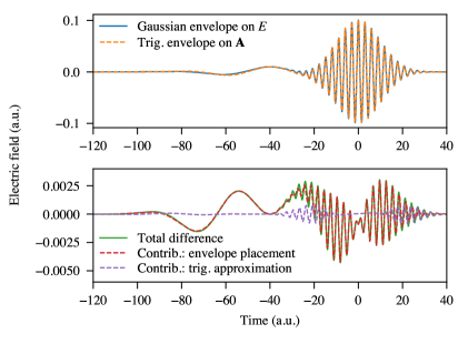
Figure 1: Top: Electric field with a Gaussian envelope on the electric field and trigonometric envelope on the vector potential with exponent $n=19$. Bottom: the difference between the two pulses and contributions to it from two distinct sources.

Fig. 2 shows the TDCCSD dipole spectra generated with the two alternative setups.

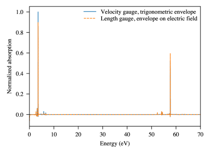
Figure 2: Difference between TDCCSD pump-probe spectra computed in the electric-dipole approximation in length gauge using the Gaussian envelope placed on the electric field, and in velocity gauge with the trigonometric envelope ($n=19$) on the vector potential.

The length-gauge spectrum is identical to that reported by Skeidsvoll et al. Skeidsvoll et al. (2020), and although differences are visible on the scale of the plot, we conclude that the velocity-gauge spectrum conveys the same physics.

Acknowledging the differences between the two setups, we will now focus on the difference between the simulations with and without the dipole approximation. Figure 3 compares the pump-probe spectrum simulated in the dipole approximation and with a plane-wave operator generated with equations (38) and (37), respectively.

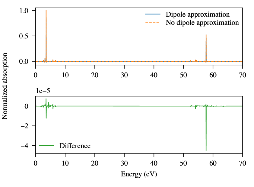
Figure 3: Top: pump-probe spectrum of LiH using the TDCCSD method in the dipole approximation and with a plane-wave operator using the aug-cc-pCVDZ basis set. Bottom: the absolute difference between the spectra generated from simulations in the dipole approximation and with the plane-wave operator.

Evidently, beyond-dipole effects are utterly negligible in this case: The simulation with the plane-wave operator produces a spectrum with the same transition frequencies as the velocity-gauge electric-dipole simulations, deviating by at most $4.5\times 10^{-5}$, corresponding to 0.0087 %, in relative intensity.

III.3 K pre-edge quadrupole transitions in Ti

For heavier elements, the bound core-valence excitations move up in energy and the shorter wavelengths become comparable to the “size” of the atoms in terms of, e.g., covalent atomic radii. This implies that higher-order multipole effects become visible in high-resolution spectra. The K-edge of Ti is expected at just below $5000\,\text{eV}$. This corresponds to a wavelength of roughly $2.5\,\text{\AA}$ which is comparable to the covalent radius of Ti ($1.60\,\text{\AA}$ Cordero et al. (2008)). Consequently, one can expect visible beyond-dipole effects even in the low-intensity limit.

We consider the Ti⁴⁺ ion and the TiCl₄ molecule. In the Ti⁴⁺ ion the $1\text{s}\rightarrow 3\text{d}$ transition is dipole forbidden but quadrupole allowed. In TiCl₄ the tetrahedral symmetry splits the $3\text{d}$-orbitals into groups of two e orbitals and three $\text{t}_{2}$ orbitals. The $1\text{s}\rightarrow\text{e}$ transition is dipole-forbidden but quadrupole-allowed, while the $1\text{s}\rightarrow\text{t}_{2}$ transition attains a dominant electric-dipole contribution due to $4\text{p}$–$3\text{d}$ mixing. Experimentally DeBeer George et al. (2005), a broad peak around $\!4969\,\text{eV}$ in the X-ray absorption spectrum of TiCl₄ has been assigned to the $1\text{s}\rightarrow\text{t}_{2}$ and $1\text{s}\rightarrow\text{e}$ with most of the intensity stemming from the former. In the implementation presented in this paper, electric-quadrupole and other higher-order contributions from the electromagnetic field should automatically be accounted for.

For both the Ti⁴⁺ and TiCl₄ systems, we perform simulations with a $10$-cycle pulse with $n=2$ for the envelope, Eq. (20), carrier frequency $181\,\text{a.u.}$ ($4925.26\,\text{eV}$), and carrier-envelope phase $\gamma=0$. The duration of the simulation is $100\,\text{a.u.}$ for Ti⁴⁺, while for TiCl₄ we use a total simulation time of $600\,\text{a.u.}$ to ensure a reasonable resolution of the splitting of the d-orbitals. The electric-field strength is $E_{1}=0.01\,\text{a.u.}$ (peak intensity $3.51\times 10^{12}\,\text{W/cm}^{2}$) and time step $\Delta t=2.5\times 10^{-4}\,\text{a.u.}$ Linearly polarized along the $x$-axis, the pulse is propagated along the $z$-axis (parallel to one of the four Ti–Cl bonds in the case of TiCl₄). All Ti⁴⁺ spectra are normalized relative to the maximum peak in the TDCCSD spectrum.

We first consider the $1\text{s}\rightarrow 4\text{p}$ and $1\text{s}\rightarrow 3\text{d}$ transitions of Ti⁴⁺, which have been studied recently at the equation-of-motion coupled-cluster singles and doubles (EOM-CCSD) level of theory by Park et al. Park et al. (2021) using multipole expansion up to electric octupole/magnetic quadrupole terms, for the full second-order contribution in the ”mixed” length and velocity gauge Sørensen et al. (2017b); Khamesian et al. (2019); Sørensen et al. (2017a), in the framework of the Fermi golden rule. In order to compare with their results, we use the ANO-RCC-VDZ basis set Roos et al. (2005). Figure 4 displays the K pre-edge spectrum obtained for Ti⁴⁺ with the TDCC2, TDOMP2, TDCCSD, and OATDCCD methods, showing also the transition frequencies obtained by Park et al. Park et al. (2021).

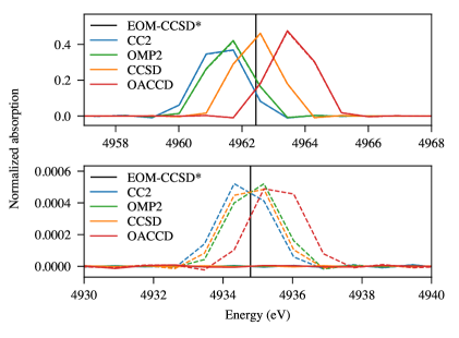
Figure 4: Ti⁴⁺ K pre-edge spectrum obtained from simulations with the ANO-RCC-VDZ basis set. Solid lines are obtained with the velocity-gauge electric-dipole approximation, while dashed lines are obtained with the plane-wave operator. Top: The dipole-allowed $1\text{s}\rightarrow 4\text{p}$ transition. Bottom: The quadrupole-allowed $1\text{s}\rightarrow 3\text{d}$ transition. Vertical black lines indicate the EOM-CCSD frequencies reported by Park et al. Park et al. (2021). Note that, although difficult to see, the dashed lines are present also in the top panel.

To within the spectral resolution of the simulation, the TDCCSD method predicts the same transition frequencies as the static EOM-CCSD method, as expected. The intensity of the dipole-allowed $1\text{s}\rightarrow 4\text{p}$ transition is very nearly the same both with and without the dipole approximation. The orbital-adaptive methods yield roughly the same intensity profiles as their static-orbital counterparts, but the transition frequencies are blue-shifted: $\sim\!0.5\,\text{eV}$ for TDOMP2 versus TDCC2 and $\sim\!2\,\text{eV}$ for OATDCCD versus TDCCSD. As has been observed previously Kristiansen et al. (2022), these blue-shifts are insignificant compared with other sources of error such as basis-set incompleteness and higher-order correlation effects. Electron-correlation effects are significantly more important than the orbital relaxation provided by dynamic orbitals, as seen in Fig. 5 where the TDCCSD spectrum is compared to the spectra obtained with the TDHF and TDCIS methods.

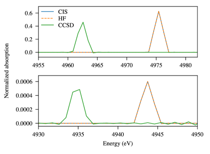
Figure 5: Ti⁴⁺ K pre-edge spectrum obtained from simulations with the plane-wave operator. Top: The dipole-allowed $1\text{s}\rightarrow 4\text{p}$ transition. Bottom: The quadrupole-allowed $1\text{s}\rightarrow 3\text{d}$ transition.

While the TDHF and TDCIS simulations produce virtually identical spectra, electron correlation causes a red-shift of the transition frequencies by roughly $8\,\text{eV}$. The TDHF and TDCIS intensities are comparable to but slightly higher than the TDCCSD ones. The main source of error, besides relativistic effects, is the choice of basis set: Changing from the ANO-RCC-VDZ basis set to the cc-pVTZ basis set increases the EOM-CCSD transition frequencies by more than $28\,\text{eV}$ Park et al. (2021).

Since we are not aiming at prediction or interpretation of experimental results in this work, we study the TiCl₄ K pre-edge spectrum using the most affordable TDCIS method with the ANO-RCC-VDZ basis set. The TDCIS spectrum is shown in Fig. 6.

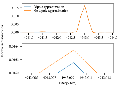
Figure 6: TiCl₄ K pre-edge spectrum from a TDCIS simulation with the plane-wave operator and with the velocity-gauge electric-dipole approximation. Top: the dipole-forbidden $1\text{s}\rightarrow\text{e}$ transition at $4941.50\,\text{eV}$ and the $1\text{s}\rightarrow\text{t}_{2}$ transition at $4942.99\,\text{eV}$. Bottom: zoomed in at the $1\text{s}\rightarrow\text{t}_{2}$ peak.

The dipole-forbidden $1\text{s}\rightarrow\text{e}$ transition is visible at $4941.50\,\text{eV}$, roughly $1.5\,\text{eV}$ below the dipole-allowed $1\text{s}\rightarrow\text{t}_{2}$ transition at $4942.99\,\text{eV}$. The TDCIS frequencies are blue-shifted by approximately $12\,\text{eV}$ relative to the EOM-CCSD results reported by Park et al. Park et al. (2021). The $1\text{s}\rightarrow\text{t}_{2}$ transition has a slightly higher intensity with the plane-wave interaction operator than with the dipole interaction operator. It should also be noted, however, that the intensities of the dipole-allowed transitions typically are slightly higher with the dipole approximation and, therefore, one should be careful using the dipole result as a reference for evaluating the quadrupole contribution. The deviation may be caused by a difference in the quality of the operator representation or the wave function, which may occur when propagating with different operators in a finite basis set.

III.4 Anisotropic circular dichroism

Circular dichroism (CD)—the difference in absorption of left and right circularly polarized radiation exhibited by chiral molecules—is a particularly interesting case to test the implementation of the beyond-dipole interaction, since the observed effect cannot be explained within the electric-dipole approximation. At least electric quadrupole and magnetic dipole terms must be included Rosenfeld (1929); Barron (2004); Pecul and Ruud (2005); Crawford (2006) and, consequently, the differential absorption is weak compared with linear, electric-dipole absorption. Chiroptical spectroscopies, including CD, are important for determining the absolute configuration of chiral molecules and core-resonant CD is particularly well suited to gauge local molecular chirality Zhang et al. (2017). As Eq. (37) was derived assuming complex polarization vectors, the implementation presented here can easily be used to generate spectra involving pulses with circular (or, more general, elliptical) polarization, including at short wavelengths.

As alluded to above, the leading contributions to a CD spectrum arise from the magnetic-dipole and electric-quadrupole terms in the multipole expansion of the vector potential. In an isotropic sample, the quadrupole contribution vanishes since the electric dipole–electric quadrupole component of the rotatory strength tensor is traceless Pedersen and Hansen (1995). As a prototypical example which previously has been used to test new implementations of CD spectra Rizzo et al. (2006); Friese and Ruud (2016); Scott et al. (2021), we will consider the H₂O₂ molecule in a chiral conformation with fixed orientation relative to the external laser pulse.

The CD spectrum is calculated as the difference between the spectral response functions of two distinct simulations: one with left circular polarization and one with right circular polarization of the pulse. We define the normalized differential absorption as

$$\bar{S}_{l-r}(\omega)=\bar{S}_{l}(\omega)-\bar{S}_{r}(\omega)$$ (43)

where $\bar{S}_{l}(\omega)$ and $\bar{S}_{r}(\omega)$ are the normalized spectral response functions for the left and right circularly polarized pulses.

The molecular geometry of H₂O₂, depicted in Fig. 7 along with the Cartesian axis definitions,

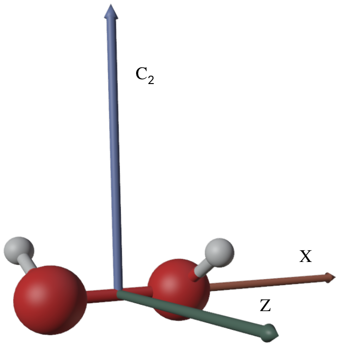
Figure 7: Definition of Cartesian coordinate system for H₂O₂ (C₂ point group).

is taken from Ref. 86. The Cartesian coordinates can be found in the supplementary material. We choose the polarization vectors such that $\bm{u}^{l}+\bm{u}^{r}=\hat{\bm{j}}$, where $\hat{\bm{j}}$ is a unit vector aligned with the C₂ axis and superscripts $r$ and $l$ refer to right and left circular polarization, respectively, as seen from the source. We run two pairs of simulations with the propagation direction along the $x$-axis and along the $z$-axis. For the propagation direction along the $x$-axis we use $\bm{u}^{r}=(0,1,\mathrm{i})$ and $\bm{u}^{l}=(0,1,-\mathrm{i})$, and for the propagation direction along the $z$-axis we use $\bm{u}^{r}=(-\mathrm{i},1,0)$ and $\bm{u}^{l}=(\mathrm{i},1,0)$. We use a carrier frequency in the K-edge region of oxygen, $\omega=20\,\text{a.u.}$ ($544.23\,\text{eV}$), and carrier-envelope phase $\gamma=0$. The duration of the laser pulse is $10$ optical cycles and the trigonometric envelope is defined with $n=2$, which corresponds to $\tau=1.14\,\text{a.u.}$. The electric-field strength is $E_{1}=0.01\,\text{a.u.}$ (peak intensity $3.51\times 10^{12}\,\text{W/cm}^{2}$) and the carrier-envelope phase is $\gamma=0$. The time step is $\Delta t=0.005\,\text{a.u.}$ and the total simulation time is $1000\,\text{a.u.}$ We use the TDHF, TDCIS, TDCC2, TDOMP2, and TDCCSD methods with the cc-pVDZ basis setDunning (1989); Woon and Dunning (1993), and the spectra for propagation direction along the $x$- and $z$-axes are normalized with respect to the corresponding TDCIS simulation.

The resulting CD spectra are plotted in Figs. 8 and 9.

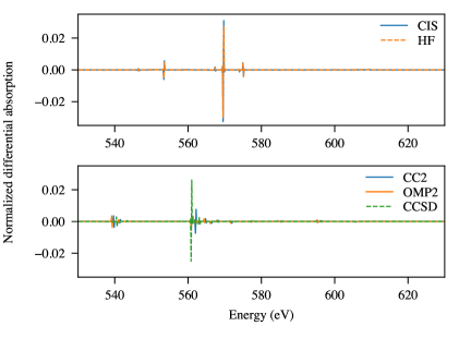
Figure 8: Differential spectra obtained with the cc-pVDZ basis set in the K-edge region of H₂O₂ with propagation direction along the $x$-axis.

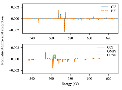
Figure 9: Differential spectra obtained with the cc-pVDZ basis set in the K-edge region of H₂O₂ with propagation direction along the $z$-axis.

As in the Ti⁴⁺ simulations above, we see that the TDCIS and TDHF methods produce nearly identical CD spectra with minor visual differences. The TDCC2 and TDOMP2 methods also yield similar CD spectra, producing the same sign pattern of the differential absorption peaks, although the TDOMP2 peak positions are slightly more red-shifted than the TDCC2 ones relative to the TDHF peaks. The intensities of the TDCC2 and TDOMP2 spectra are significantly reduced compared with the TDHF and TDCIS spectra. The TDCCSD method shifts the transition frequencies somewhat but produces an intensity of the dominant peak around $561$-$562\,\text{eV}$ which is closer to that of TDHF theory than the TDCC2 and TDOMP2 methods. Although this may indicate that high-level electron-correlation treatment is important, the deviation may also be caused by limited frequency resolution (see below). Of course, the choice of carrier frequency will affect the relative peak magnitudes but further tests have shown that this effect is rather marginal as long as $\omega$ is reasonably close to the transition energies.

Figure 10 shows the CD spectrum obtained from the TDCIS simulations along with a stick spectrum calculated from the rotatory strength tensors Pedersen and Hansen (1995) computed by full diagonalization of the CIS Hamiltonian matrix.

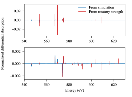
Figure 10: Differential spectra obtained with the cc-pVDZ basis set in the K-edge region of H₂O₂ with propagation direction along the $x$ (top) and $z$ (bottom) axes, along with circular dichroism calculated from rotatory strengths.

For both propagation directions, the stick spectrum is normalized such that the maximum peak is equal to the maximum peak from the corresponding TDCIS simulation. Since the carrier frequency is $544.23\,\text{eV}$, it is expected that the peaks of the stick spectrum are smaller than the simulated peaks to the immediate left of the dominant peak, and larger further to the right of the dominant peak. This is indeed what we observe in the bottom panel of Fig. 10. In the top panel, however, this is not the case. This can be ascribed to insufficient convergence. The excited states of H₂O₂ in the C₂ geometry come in pairs, typically separated by 0.01 eV or less, formed by the lowering of symmetry relative to a planar, achiral (cis or trans) structure. For propagation in the $x$-direction, the CD for these pairs of states are of about the same magnitude but with opposite signs, causing lowering of the peak intensities. Figure 11 shows the effect of increasing the simulation time from $1000\,\text{a.u.}$ to $7500\,\text{a.u.}$ The change in the bottom panel is relatively minor, while the dominant peak in the top panel has increased by an order of magnitude. This is closer to the expected difference calculated from rotatory strength tensors. However, the peak at $567\,\text{eV}$ is still much suppressed, which is caused by the states only being separated by about $0.0088\,\text{eV}$.

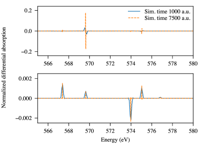
Figure 11: TDCIS differential spectra obtained with the cc-pVDZ basis set in the K-edge region of H₂O₂ with propagation direction along the $x$ (top) and $z$ (bottom) axes, with simulation times of $1000\,\text{a.u.}$ and $7500\,\text{a.u.}$

An overview of the occupied orbitals and the $11$ lowest-lying virtual orbitals is given in Table 1.

Table 1: Occupied orbitals and the $11$ lowest-lying virtual orbitals of H₂O₂ with the cc-pVDZ basis set. The orbital types are based on similarity with the peroxide ion. Due to the reduced symmetry, all orbitals are somewhat mixed.

No.	Energy (a.u.)	Symmetry label	Type
1	-561.27036	1A	$\sigma$
2	-561.26301	1B	$\sigma^{*}$
3	-39.992527	2A	$\sigma$
4	-33.108905	2B	$\sigma$
5	-19.465831	3B	$\pi_{z}$
6	-18.833153	3A	$\pi_{y}$
7	-16.202217	4A	$\sigma_{p_{x}}$
8	-14.251659	5A	$\pi_{z}^{*}$
9	-13.038506	4B	$\pi_{y}^{*}$
10	5.1526056	6A	$\sigma$
11	5.2866155	5B	$\sigma^{*}$
12	7.7990137	6B	$\sigma_{p_{x}}^{*}$
13	22.642558	7A	Mixed, dominant weight on H
14	22.835716	7B	Mixed, dominant weight on H
15	30.276955	8B	$\sigma^{*}_{s/p_{x}}$
16	30.673602	8A	$\pi_{y}$/$\pi_{z}^{*}$
17	31.260347	9A	$\pi_{z}^{*}$
18	32.689754	9B	$\sigma^{*}_{p_{x}}$/$pi_{y}^{*}$
19	34.770868	10B	Mixed $\sigma$/$\pi$
20	36.906177	10A	$\sigma^{*}_{s/p_{x}}$

The core orbitals, 1$\sigma_{s}$ and 1$\sigma_{s}^{*}$, are separated by $7.3483\times 10^{-3}~{}\text{eV}$ and, hence, excitations from either of the core orbitals to low-lying virtual orbitals will fall in the K pre-edge region. The TDCIS spectrum contains $5$ main peaks below $580\,\text{eV}$ along with three smaller ones at $553.44\,\text{eV}$, $560.24\,\text{eV}$, and $576.82\,\text{eV}$. The first peak at $546.48\,\text{eV}$ can be viewed as a transition to virtual orbitals 5B and 6B. The main peak in Fig. 8 at $569.63\,\text{eV}$ contains significant excitations to orbitals 8A, 9A and 9B, which are orbitals with significant $\pi$ character, and with electron density mostly located on the oxygen atoms. The main peak in Fig. 9 at $573.97\,\text{eV}$ is mainly due to excitations to the 7B and 8B (and somewhat to 10A) orbitals.

Finally, noting that the cc-pVDZ basis set is insufficient for accurate predictions of CD spectra in general—see, e.g., Ref. 83— we compare the TDCIS spectra with those obtained with larger basis sets in Fig. 12.

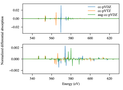
Figure 12: TDCIS CD spectra in the K-edge region of H₂O₂ with propagation direction along the $x$-axis (top) and $z$-axis (bottom).

As expected, the basis-set effect is significant. Going from double-zeta to triple-zeta basis retains some of the main features but the energies are red-shifted, whereas the inclusion of diffuse orbitals in the aug-cc-pVDZ basis set leads to a much more radical change of the underlying dynamics due to a higher density of excited states in the energy region around the carrier frequency. More accurate predictions of transient CD spectra, especially with the higher-level TDCC methods, clearly require larger basis sets including diffuse functions.

IV Concluding remarks

We have derived a gauge invariant expression for the spectral response function which is applicable to transient absorption and emission spectra. This expression is applicable both within and beyond the electric-dipole approximation. Using an enveloped plane-wave vector potential to formulate the semiclassical matter-field interaction operator, simulations of laser-driven many-electron dynamics with a fixed atom-centered Gaussian basis set can be straightforwardly carried out with no additional cost compared with the analogous electric-dipole simulations. Numerical experiments show that beyond-dipole effects are fully captured without explicit multipole expansions, and that electric-dipole results are correctly reproduced in the long wavelength limit. Circular (or, more general, elliptical) polarization is easily handled, as illustrated by preliminary simulations of anisotropic transient X-ray circular dichroism spectra.

Aimed at electronic ground and bound excited states, fixed atom-centered Gaussian basis sets do not support electronic continuum states and, consequently, we have only considered low-intensity laser fields in this work. We are currently extending the approach presented here to more flexible bases that allow us to study highly non-linear processes such as core ionization where the magnetic component of the electromagnetic field may play a decisive role.

V Supplementary material

The supplementary material contains the molecular geometries of LiH, TiCl₄, and H₂O₂, and a brief analysis of the differences between pulses with envelopes defined on the electric field and on the vector potential.

References

- Corkum and Krausz (2007) P. B. Corkum and F. Krausz, Attosecond science, Nat. Phys. 3, 381 (2007).
- Krausz and Ivanov (2009) F. Krausz and M. Ivanov, Attosecond physics, Rev. Mod. Phys. 81, 163 (2009).
- Nisoli et al. (2017) M. Nisoli, P. Decleva, F. Calegari, A. Palacios, and F. Martín, Attosecond Electron Dynamics in Molecules, Chem. Rev. 117, 10760 (2017).
- Klinker et al. (2018) M. Klinker, C. Marante, L. Argenti, J. González-Vázquez, and F. Martín, Electron Correlation in the Ionization Continuum of Molecules: Photoionization of N2 in the Vicinity of the Hopfield Series of Autoionizing States, J. Phys. Chem. Lett. , 756 (2018).
- Kulander (1988) K. C. Kulander, Time-dependent theory of multiphoton ionization of xenon, Phys. Rev. A 38, 778 (1988).
- Schafer and Kulander (1990) K. J. Schafer and K. C. Kulander, Energy analysis of time-dependent wave functions: Application to above-threshold ionization, Phys. Rev. A 42, 5794 (1990).
- Kulander et al. (1993) K. C. Kulander, K. J. Schafer, and J. L. Krause, Dynamics of Short-Pulse Excitation, Ionization and Harmonic Conversion, in Super-Intense Laser-Atom Physics, NATO ASI Series, edited by B. Piraux, A. L’Huillier, and K. Rza̧żewski (Springer US, Boston, MA, 1993) pp. 95–110.
- Lezius et al. (2001) M. Lezius, V. Blanchet, D. M. Rayner, D. M. Villeneuve, A. Stolow, and M. Y. Ivanov, Nonadiabatic Multielectron Dynamics in Strong Field Molecular Ionization, Phys. Rev. Lett. 86, 51 (2001).
- Markevitch et al. (2003) A. N. Markevitch, S. M. Smith, D. A. Romanov, H. Bernhard Schlegel, M. Y. Ivanov, and R. J. Levis, Nonadiabatic dynamics of polyatomic molecules and ions in strong laser fields, Phys. Rev. A 68, 011402 (2003).
- Olsen and Jørgensen (1985) J. Olsen and P. Jørgensen, Linear and nonlinear response functions for an exact state and for an MCSCF state, J. Chem. Phys. 82, 3235 (1985).
- List et al. (2015) N. H. List, J. Kauczor, T. Saue, H. J. A. Jensen, and P. Norman, Beyond the electric-dipole approximation: A formulation and implementation of molecular response theory for the description of absorption of electromagnetic field radiation, J. Chem. Phys. 142, 244111 (2015).
- List et al. (2017) N. H. List, T. Saue, and P. Norman, Rotationally averaged linear absorption spectra beyond the electric-dipole approximation, Mol. Phys. 115, 63 (2017).
- Sørensen et al. (2019) L. K. Sørensen, E. Kieri, S. Srivastav, M. Lundberg, and R. Lindh, Implementation of a semiclassical light-matter interaction using the Gauss-Hermite quadrature: A simple alternative to the multipole expansion, Phys. Rev. A 99, 10.1103/PhysRevA.99.013419 (2019).
- van Horn et al. (2022) M. van Horn, T. Saue, and N. H. List, Probing chirality across the electromagnetic spectrum with the full semi-classical light–matter interaction, J. Chem. Phys. 156, 054113 (2022).
- Bernadotte et al. (2012) S. Bernadotte, A. J. Atkins, and C. R. Jacob, Origin-independent calculation of quadrupole intensities in X-ray spectroscopy, J. Chem. Phys. 137, 204106 (2012).
- Lestrange et al. (2015) P. J. Lestrange, F. Egidi, and X. Li, The consequences of improperly describing oscillator strengths beyond the electric dipole approximation, J. Chem. Phys. 143, 234103 (2015).
- Sørensen et al. (2017a) L. K. Sørensen, R. Lindh, and M. Lundberg, Gauge origin independence in finite basis sets and perturbation theory, Chem. Phys. Lett. 683, 536 (2017a).
- van Horn et al. (2023) M. van Horn, N. H. List, and T. Saue, Transition moments beyond the electric-dipole approximation: Visualization and basis set requirements, J. Chem. Phys. 158, 184103 (2023).
- Wu et al. (2016) M. Wu, S. Chen, S. Camp, K. J. Schafer, and M. B. Gaarde, Theory of strong-field attosecond transient absorption, J. Phys. B 49, 62003 (2016).
- Rohringer et al. (2006) N. Rohringer, A. Gordon, and R. Santra, Configuration-interaction-based time-dependent orbital approach for ab initio treatment of electronic dynamics in a strong optical laser field, Phys. Rev. A 74, 043420 (2006).
- Krause et al. (2007) P. Krause, T. Klamroth, and P. Saalfrank, Molecular response properties from explicitly time-dependent configuration interaction methods, J. Chem. Phys. 127, 034107 (2007).
- Schlegel et al. (2007) H. B. Schlegel, S. M. Smith, and X. Li, Electronic optical response of molecules in intense fields: Comparison of TD-HF, TD-CIS, and TD-CIS(D) approaches, J. Chem. Phys. 126, 244110 (2007).
- Pabst et al. (2011) S. Pabst, L. Greenman, P. J. Ho, D. A. Mazziotti, and R. Santra, Decoherence in Attosecond Photoionization, Phys. Rev. Lett. 106, 053003 (2011).
- White et al. (2016) A. F. White, C. J. Heide, P. Saalfrank, M. Head-Gordon, and E. Luppi, Computation of high-harmonic generation spectra of the hydrogen molecule using time-dependent configuration-interaction, Mol. Phys. 114, 947 (2016).
- Ofstad et al. (2023) B. S. Ofstad, E. Aurbakken, Ø. S. Schøyen, H. E. Kristiansen, S. Kvaal, and T. B. Pedersen, Time-dependent coupled-cluster theory, WIREs Comput. Mol. Sci. , e1666 (2023), in press; available online.
- Kfir et al. (2015) O. Kfir, P. Grychtol, E. Turgut, R. Knut, D. Zusin, D. Popmintchev, T. Popmintchev, H. Nembach, J. M. Shaw, A. Fleischer, H. Kapteyn, M. Murnane, and O. Cohen, Generation of bright phase-matched circularly-polarized extreme ultraviolet high harmonics, Nat. Photon. 9, 99 (2015).
- Bandrauk and Yuan (2016) A. D. Bandrauk and K.-J. Yuan, Circularly polarised attosecond pulses: generation and applications, Mol. Phys. 114, 344 (2016).
- Shao et al. (2020) R. Shao, C. Zhai, Y. Zhang, N. Sun, W. Cao, P. Lan, and P. Lu, Generation of isolated circularly polarized attosecond pulses by three-color laser field mixing, Opt. Express 28, 15874 (2020).
- Ma et al. (2016) G. Ma, W. Yu, M. Y. Yu, B. Shen, and L. Veisz, Intense circularly polarized attosecond pulse generation from relativistic laser plasmas using few-cycle laser pulses, Opt. Express 24, 10057 (2016).
- Zhong et al. (2021) C. Zhong, B. Qiao, Y. Zhang, Y. Zhang, X. Li, J. Wang, C. Zhou, S. Zhu, and X. He, Production of intense isolated attosecond pulses with circular polarization by using counter-propagating relativistic lasers, New J. Phys. 23, 063080 (2021).
- Chen et al. (2016) C. Chen, Z. Tao, C. Hernández-García, P. Matyba, A. Carr, R. Knut, O. Kfir, D. Zusin, C. Gentry, P. Grychtol, O. Cohen, L. Plaja, A. Becker, A. Jaron-Becker, H. Kapteyn, and M. Murnane, Tomographic reconstruction of circularly polarized high-harmonic fields: 3D attosecond metrology, Sci. Adv. 2, e1501333 (2016).
- Pedersen and Hansen (1995) T. B. Pedersen and A. E. Hansen, Ab initio calculation and display of the rotatory strength tensor in the random phase approximation: Method and model studies, Chem. Phys. Lett. 246, 1 (1995).
- Jackson (1975) J. D. Jackson, Classical Electrodynamics, 2nd ed. (Wiley, New York, 1975).
- Weyl (1927) H. Weyl, Quantenmechanik und Gruppentheorie, Z. Phys. 46, 1 (1927).
- Tannor (2007) D. J. Tannor, Introduction to quantum mechanics: A time-dependent perspective (University Science Books, Sausalito, Calif, 2007).
- Skeidsvoll et al. (2020) A. S. Skeidsvoll, A. Balbi, and H. Koch, Time-dependent coupled-cluster theory for ultrafast transient-absorption spectroscopy, Phys. Rev. A 102, 023115 (2020).
- Guandalini et al. (2021) A. Guandalini, C. Cocchi, S. Pittalis, A. Ruini, and C. A. Rozzi, Nonlinear light absorption in many-electron systems excited by an instantaneous electric field: a non-perturbative approach, Phys. Chem. Chem. Phys. 23, 10059 (2021).
- Goldstein (1980) H. Goldstein, Classical Mechanics, 2nd ed. (Addison-Wesley, Reading, MA, 1980).
- Yang (1976a) K.-H. Yang, Gauge transformations and quantum mechanics I. Gauge invariant interpretation of quantum mechanics, Ann. Phys. 101, 62 (1976a).
- Kobe and Yang (1987) D. H. Kobe and K.-H. Yang, Energy of a classical charged particle in an external electromagnetic field, Eur. J. Phys. 8, 236 (1987).
- Yang (1976b) K.-H. Yang, Gauge transformations and quantum mechanics II. Physical interpretation of classical gauge transformations, Ann. Phys. 101, 97 (1976b).
- Kobe and Smirl (1978) D. H. Kobe and A. L. Smirl, Gauge invariant formulation of the interaction of electromagnetic radiation and matter, Am. J. Phys. 46, 624 (1978).
- Kobe (1978) D. H. Kobe, Implications of gauge invariance for length versus velocity forms of the interaction with electric dipole radiation, Int. J. Quantum Chem. 14, 73 (1978).
- Kobe and Yang (1980) D. H. Kobe and K.-H. Yang, Gauge-invariant non-relativistic limit of an electron in a time-dependent electromagnetic field, J. Phys. A 13, 3171 (1980).
- Aharonov and Au (1981) Y. Aharonov and C. K. Au, The question of gauge dependence of transition probabilities in quantum mechanics: Facts, myths and misunderstandings, Phys. Lett. A 86, 269 (1981).
- Kobe and Wen (1982) D. H. Kobe and E. C. T. Wen, Gauge invariance in quantum mechanics: Charged harmonic oscillator in an electromagnetic field, J. Phys. A 15, 787 (1982).
- Schlicher et al. (1984) R. R. Schlicher, W. Becker, J. Bergou, and M. O. Scully, Interaction Hamiltonian in Quantum Optics Or: vs. Revisited, in Quantum Electrodynamics and Quantum Optics, NATO ASI Series, edited by A. O. Barut (Springer US, Boston, MA, 1984) pp. 405–441.
- Barth and Lasser (2009) I. Barth and C. Lasser, Trigonometric pulse envelopes for laser-induced quantum dynamics, J. Phys. B 42, 235101 (2009).
- Rauch and Mourou (2006) J. Rauch and G. Mourou, The time integrated far field for Maxwell’s and D’Alembert’s equations, Proc. Am. Math. Soc. 134, 851 (2006).
- Førre et al. (2005) M. Førre, S. Selstø, J. P. Hansen, and L. B. Madsen, Exact Nondipole Kramers-Henneberger Form of the Light-Atom Hamiltonian: An Application to Atomic Stabilization and Photoelectron Energy Spectra, Phys. Rev. Lett. 95, 043601 (2005).
- Førre et al. (2006) M. Førre, J. P. Hansen, L. Kocbach, S. Selstø, and L. B. Madsen, Nondipole ionization dynamics of atoms in superintense high-frequency attosecond pulses, Phys. Rev. Lett. 97, 043601 (2006).
- Moe and Førre (2018) T. E. Moe and M. Førre, Ionization of atomic hydrogen by an intense x-ray laser pulse: An ab initio study of the breakdown of the dipole approximation, Phys. Rev. A 97, 10.1103/PhysRevA.97.013415 (2018).
- Aurbakken, E. and Fredly, K. H. and Kristiansen, H. E. and Kvaal, S. and Myhre, R. H. and Ofstad, B. S. and Pedersen, T. B. and Schøyen, Ø. S. and Sutterud, H. and Winther-Larsen, S. G. (2 04) Aurbakken, E. and Fredly, K. H. and Kristiansen, H. E. and Kvaal, S. and Myhre, R. H. and Ofstad, B. S. and Pedersen, T. B. and Schøyen, Ø. S. and Sutterud, H. and Winther-Larsen, S. G., HyQD: Hylleraas Quantum Dynamics (2023-02-04), URL: https://github.com/HyQD.
- Li et al. (2020) X. Li, N. Govind, C. Isborn, A. E. DePrince, and K. Lopata, Real-Time Time-Dependent Electronic Structure Theory, Chem. Rev. 120, 9951 (2020).
- Christiansen et al. (1995) O. Christiansen, H. Koch, and P. Jørgensen, The second-order approximate coupled cluster singles and doubles model CC2, Chem. Phys. Lett. 243, 409 (1995).
- Kristiansen et al. (2022) H. E. Kristiansen, B. S. Ofstad, E. Hauge, E. Aurbakken, Ø. S. Schøyen, S. Kvaal, and T. B. Pedersen, Linear and Nonlinear Optical Properties from TDOMP2 Theory, J. Chem. Theory Comput. 18, 3687 (2022).
- Pedersen and Kvaal (2019) T. B. Pedersen and S. Kvaal, Symplectic integration and physical interpretation of time-dependent coupled-cluster theory, J. Chem. Phys. 150, 144106 (2019).
- Pathak et al. (2020) H. Pathak, T. Sato, and K. L. Ishikawa, Time-dependent optimized coupled-cluster method for multielectron dynamics. II. A coupled electron-pair approximation, J. Chem. Phys. 152, 124115 (2020).
- Kvaal (2012) S. Kvaal, Ab initio quantum dynamics using coupled-cluster, J. Chem. Phys. 136, 194109 (2012).
- Pedersen and Koch (1997) T. B. Pedersen and H. Koch, Coupled cluster response functions revisited, J. Chem. Phys. 106, 8059 (1997).
- Pedersen and Koch (1998) T. B. Pedersen and H. Koch, Gauge invariance of the coupled cluster oscillator strength, Chem. Phys. Lett. 293, 251 (1998).
- Pedersen et al. (1999) T. B. Pedersen, H. Koch, and C. Hättig, Gauge invariant coupled cluster response theory, J. Chem. Phys. 110, 8318 (1999).
- Pedersen et al. (2001) T. B. Pedersen, B. Fernández, and H. Koch, Gauge invariant coupled cluster response theory using optimized nonorthogonal orbitals, J. Chem. Phys. 114, 6983 (2001).
- Sato et al. (2018) T. Sato, H. Pathak, Y. Orimo, and K. L. Ishikawa, Communication: Time-dependent optimized coupled-cluster method for multielectron dynamics, J. Chem. Phys. 148, 051101 (2018).
- Fdez. Galván et al. (2019) I. Fdez. Galván, M. Vacher, A. Alavi, C. Angeli, F. Aquilante, J. Autschbach, J. J. Bao, S. I. Bokarev, N. A. Bogdanov, R. K. Carlson, L. F. Chibotaru, J. Creutzberg, N. Dattani, M. G. Delcey, S. S. Dong, A. Dreuw, L. Freitag, L. M. Frutos, L. Gagliardi, F. Gendron, A. Giussani, L. González, G. Grell, M. Guo, C. E. Hoyer, M. Johansson, S. Keller, S. Knecht, G. Kovačević, E. Källman, G. Li Manni, M. Lundberg, Y. Ma, S. Mai, J. P. Malhado, P. Å. Malmqvist, P. Marquetand, S. A. Mewes, J. Norell, M. Olivucci, M. Oppel, Q. M. Phung, K. Pierloot, F. Plasser, M. Reiher, A. M. Sand, I. Schapiro, P. Sharma, C. J. Stein, L. K. Sørensen, D. G. Truhlar, M. Ugandi, L. Ungur, A. Valentini, S. Vancoillie, V. Veryazov, O. Weser, T. A. Wesołowski, P.-O. Widmark, S. Wouters, A. Zech, J. P. Zobel, and R. Lindh, OpenMolcas: From Source Code to Insight, J. Chem. Theory Comput. 15, 5925 (2019).
- Aquilante et al. (2020) F. Aquilante, J. Autschbach, A. Baiardi, S. Battaglia, V. A. Borin, L. F. Chibotaru, I. Conti, L. De Vico, M. Delcey, I. Fdez. Galván, N. Ferré, L. Freitag, M. Garavelli, X. Gong, S. Knecht, E. D. Larsson, R. Lindh, M. Lundberg, P. Å. Malmqvist, A. Nenov, J. Norell, M. Odelius, M. Olivucci, T. B. Pedersen, L. Pedraza-González, Q. M. Phung, K. Pierloot, M. Reiher, I. Schapiro, J. Segarra-Martí, F. Segatta, L. Seijo, S. Sen, D. Sergentu, C. J. Stein, L. Ungur, M. Vacher, A. Valentini, and V. Veryazov, Modern quantum chemistry with [Open]Molcas, J. Chem. Phys. 152, 214117 (2020).
- Olsen et al. (2020) J. M. H. Olsen, S. Reine, O. Vahtras, E. Kjellgren, P. Reinholdt, K. O. H. Dundas, X. Li, J. Cukras, M. Ringholm, E. D. Hedegård, R. Di Remigio, N. H. List, R. Faber, B. N. C. Tenorio, R. Bast, T. B. Pedersen, Z. Rinkevicius, S. P. A. Sauer, K. V. Mikkelsen, J. Kongsted, S. Coriani, K. Ruud, T. Helgaker, H. J. A. Jensen, and P. Norman, Dalton Project: A Python platform for molecular- and electronic-structure simulations of complex systems, J. Chem. Phys. 152, 214115 (2020).
- Sun et al. (2018) Q. Sun, T. C. Berkelbach, N. S. Blunt, G. H. Booth, S. Guo, Z. Li, J. Liu, J. D. McClain, E. R. Sayfutyarova, S. Sharma, S. Wouters, and G. K. Chan, PySCF: the Python‐based simulations of chemistry framework, WIREs Comput. Mol. Sci 8, e1340 (2018).
- Aidas et al. (2014) K. Aidas, C. Angeli, K. L. Bak, V. Bakken, R. Bast, L. Boman, O. Christiansen, R. Cimiraglia, S. Coriani, P. Dahle, E. K. Dalskov, U. Ekström, T. Enevoldsen, J. J. Eriksen, P. Ettenhuber, B. Fernández, L. Ferrighi, H. Fliegl, L. Frediani, K. Hald, A. Halkier, C. Hättig, H. Heiberg, T. Helgaker, A. C. Hennum, H. Hettema, E. Hjertenæs, S. Høst, I. Høyvik, M. F. Iozzi, B. Jansík, H. Jensen, D. Jonsson, P. Jørgensen, J. Kauczor, S. Kirpekar, T. Kjærgaard, W. Klopper, S. Knecht, R. Kobayashi, H. Koch, J. Kongsted, A. Krapp, K. Kristensen, A. Ligabue, O. B. Lutnæs, J. I. Melo, K. V. Mikkelsen, R. H. Myhre, C. Neiss, C. B. Nielsen, P. Norman, J. Olsen, J. M. H. Olsen, A. Osted, M. J. Packer, F. Pawlowski, T. B. Pedersen, P. F. Provasi, S. Reine, Z. Rinkevicius, T. A. Ruden, K. Ruud, V. V. Rybkin, P. Sałek, C. C. M. Samson, A. Sánchez de Merás, T. Saue, S. P. A. Sauer, B. Schimmelpfennig, K. Sneskov, A. H. Steindal, K. O. Sylvester-Hvid, P. R. Taylor, A. M. Teale, E. I. Tellgren, D. P. Tew, A. J. Thorvaldsen, L. Thøgersen, O. Vahtras, M. A. Watson, D. J. D. Wilson, M. Ziolkowski, and H. Ågren, The Dalton quantum chemistry program system, WIREs Comput. Mol. Sci. 4, 269 (2014).
- Pritchard et al. (2019) B. P. Pritchard, D. Altarawy, B. Didier, T. D. Gibsom, and T. L. Windus, A New Basis Set Exchange: An Open, Up-to-date Resource for the Molecular Sciences Community, J. Chem. Inf. Model. 59, 4814 (2019).
- Hairer et al. (2006) E. Hairer, C. Lubich, and G. Wanner, Geometric Numerical Integration, 2nd ed. (Springer, Berlin, 2006).
- Cordero et al. (2008) B. Cordero, V. Gómez, A. E. Platero-Prats, M. Revés, J. Echeverría, E. Cremades, F. Barragán, and S. Alvarez, Covalent radii revisited, Dalton Trans. 21, 2832 (2008).
- DeBeer George et al. (2005) S. DeBeer George, P. Brant, and E. I. Solomon, Metal and Ligand K-Edge XAS of Organotitanium Complexes: Metal 4p and 3d Contributions to Pre-edge Intensity and Their Contributions to Bonding, J. Am. Chem. Soc. 127, 667 (2005).
- Park et al. (2021) Y. C. Park, A. Perera, and R. J. Bartlett, Equation of motion coupled-cluster study of core excitation spectra II: Beyond the dipole approximation, J. Chem. Phys. 155, 094103 (2021).
- Sørensen et al. (2017b) L. K. Sørensen, M. Guo, R. Lindh, and M. Lundberg, Applications to metal k pre-edges of transition metal dimers illustrate the approximate origin independence for the intensities in the length representation, Mol. Phys. 115, 174 (2017b).
- Khamesian et al. (2019) M. Khamesian, I. Galván, M. G. Delcey, L. K. Sørensen, and R. Lindh, Spectroscopy of linear and circular polarized light with the exact semiclassical light–matter interaction, in Annual Reports in Computational Chemistry, Vol. 15, edited by D. A. Dixon (Elsevier, Amsterdam, 2019) pp. 39–76.
- Roos et al. (2005) B. O. Roos, R. Lindh, P.-Å. Malmqvist, V. Veryazov, and P.-O. Widmark, New Relativistic ANO Basis Sets for Transition Metal Atoms, J. Phys. Chem. A 109, 6575 (2005).
- Rosenfeld (1929) L. Rosenfeld, Quantenmechanische Theorie der natürlichen optischen Aktivität von Flüssigkeiten und Gasen, Z. Physik 52, 161 (1929).
- Barron (2004) L. D. Barron, Molecular Light Scattering and Optical Activity, 2nd ed. (Cambridge University Press, Cambridge, 2004).
- Pecul and Ruud (2005) M. Pecul and K. Ruud, The Ab Initio Calculation of Optical Rotation and Electronic Circular Dichroism, in Advances in Quantum Chemistry, Vol. 50, edited by H. J. Å. Jensen (Academic Press, 2005) pp. 185–212.
- Crawford (2006) T. D. Crawford, Ab initio calculation of molecular chiroptical properties, Theor. Chem. Acc. 115, 227 (2006).
- Zhang et al. (2017) Y. Zhang, J. R. Rouxel, J. Autschbach, N. Govind, and S. Mukamel, X-ray circular dichroism signals: a unique probe of local molecular chirality, Chem. Sci. 8, 5969 (2017).
- Rizzo et al. (2006) A. Rizzo, B. Jansík, T. B. Pedersen, and H. Ågren, Origin invariant approaches to the calculation of two-photon circular dichroism, J. Chem. Phys. 125, 064113 (2006).
- Friese and Ruud (2016) D. H. Friese and K. Ruud, Three-photon circular dichroism: towards a generalization of chiroptical non-linear light absorption, Phys. Chem. Chem. Phys. 18, 4174 (2016).
- Scott et al. (2021) M. Scott, D. R. Rehn, S. Coriani, P. Norman, and A. Dreuw, Electronic circular dichroism spectra using the algebraic diagrammatic construction schemes of the polarization propagator up to third order, J. Chem. Phys. 154, 064107 (2021).
- Redington et al. (1962) R. L. Redington, W. B. Olson, and P. C. Cross, Studies of hydrogen peroxide: the infrared spectrum and the internal rotation problem, J. Chem. Phys. 36, 1311 (1962).
- Dunning (1989) T. H. Dunning, Gaussian basis sets for use in correlated molecular calculations. I. The atoms boron through neon and hydrogen, J. Chem. Phys. 90, 1007 (1989).
- Woon and Dunning (1993) D. E. Woon and T. H. Dunning, Gaussian basis sets for use in correlated molecular calculations. III. The atoms aluminum through argon, J. Chem. Phys. 98, 1358 (1993).