Very accurate time propagation of coupled Schrödinger equations for femto- and attosecond physics and chemistry, with C++ source code

Abstract

In this article, I present a very fast and high-precision (up to 33 decimal places) C++ implementation of the semi-global time propagation algorithm for a system of coupled Schrödinger equations with a time-dependent Hamiltonian. It can be used to describe time-dependent processes in molecular systems after excitation by femto- and attosecond laser pulses. It also works with an arbitrary user supplied Hamiltonian and can be used for nonlinear problems. The semi-global algorithm is briefly presented, the C++ implementation is described and five sample simulations are shown. The accompanying C++ source code package is included. The high precision benchmark (long double and float128) shows the estimated calculation costs. The presented method turns out to be faster and more accurate than the global Chebyshev propagator.

1 Introduction

The time-dependent Schrödinger equation (TDSE):

$$i\hbar\frac{\partial\psi}{\partial t}=\hat{\mathbf{H}}(t)\psi,$$ (1)

is essential to quantum dynamics and especially to femto- and attosecond chemistry. The equation for a system of several coupled time-dependent Schrödinger equations can be written down with explicitly shown all $n$ coupled terms inside $\psi$ and $\hat{\mathbf{H}}(t)$:

$$i\hbar\frac{\partial}{\partial t}\begin{pmatrix}{\psi}_{1}\\[2.84526pt] {\psi}_{2}\\[2.84526pt] \vdots\\[2.84526pt] {\psi}_{n}\end{pmatrix}=\begin{bmatrix}\hat{\mathbf{H}}_{1}(t)&\hat{\mathbf{V}}_{1,2}(t)&\dots&\hat{\mathbf{V}}_{1,n}(t)\\[2.84526pt] \hat{\mathbf{V}}_{2,1}(t)&\hat{\mathbf{H}}_{2}(t)&\dots&\hat{\mathbf{V}}_{2,n}(t)\\[2.84526pt] \vdots&\vdots&\ddots&\vdots\\[2.84526pt] \hat{\mathbf{V}}_{n,1}(t)&\hat{\mathbf{V}}_{n,2}(t)&\dots&\hat{\mathbf{H}}_{n}(t)\end{bmatrix}\begin{pmatrix}{\psi}_{1}\\[2.84526pt] {\psi}_{2}\\[2.84526pt] \vdots\\[2.84526pt] {\psi}_{n}\end{pmatrix}$$ (2)

Each $\psi_{n}$ corresponds to a particular wavefunction at $n$-th electronic potential, while $\hat{\mathbf{V}}_{j,k}$ correspond to the coupling elements between the corresponding levels and $\hat{\mathbf{H}}_{i}(t)$ is the Hamiltonian at a given level. The solution to such system provides us with an understanding of fundamental quantum processes. For almost all of these processes closed form solutions do not exist. Instead of these the numerical algorithms are being developed to simulate the quantum processes from first principles.

This paper describes a general semi-global algorithm for various classes of problems including time-dependent Hamiltonian, nonlinear problems, non-hermitian problems and problems with an inhomogeneous source term [1, 2, 3]. The novelty is both the C++ implementation ($10\times$ faster than Octave) of this algorithm as well as the addition of the ability to calculate multiple coupled electronic levels in high precision (long double and float128 types having 18 and 33 decimal places respectively).

The main advantage of the presented algorithm is the ability to significantly reduce the numerical error in time propagation up to the level of the Unit in the Last Place (ULP) error¹ of the floating point numerical representation (see Sections 3 and 6, compare also with [4]). This is made possible by iteratively applying the Duhamel’s principle until the required convergence criterion is met for $\hat{\mathbf{H}}(t)$. Additionally, the error tolerance can be used to control the calculation speed.

This ability to produce results with errors in the range of the numerical ULP error of used precision, together with high precision types long double (18 decimal places) and float128 (33 decimal places) and a fast C++ implementation means that the code presented in this work can be used to obtain reference results in many difficult simulation cases.

This work is divided into the following sections. In the next section the theoretical introduction to the semi-global method [1, 2, 3] is presented. In Section 3 the high-precision calculations are briefly substantiated and described. In Section 4 the technical details of the C++ implementation are discussed. In Section 5 a validation of the current implementation is performed. In Section 6 the computation speed benchmarks are presented. In Section 7 the accompanying C++ source code package is described and finally, the conclusions are in Section 8.

2 The semi-global method

The time-dependent Hamiltonian is useful for ultrafast spectroscopy, high harmonic generation or coherent control problems. In some cases the Hamiltonian may become nonlinear depending explicitly on the state $\psi(t)$. Such case occurs in mean field approximation, in the Gross-Pitaevskii approximation [5], time-dependent Hartree [6, 7, 8, 9] and time-dependent DFT [10, 11, 12, 13]. Another complication may arise when adding a source term to the Schrödinger equation, such as in scattering problems [14]. All these cases will be possible to calculate with the semi-global [2, 3, 15] method ported from Matlab/Octave [2, 3] to C++ and described in this paper.

The global scheme described in [16, 17] assumes the knowledge of the eigenvalue range of the Hamiltonian (i.e. the $E_{min}$ and $E_{max}$). Usually, such knowledge is missing, especially for time-dependent or non-Hermitian problems. To overcome this difficulty the method below is implemented with the Arnoldi approach. The main advantage of this approach is that the algorithm determines the energy range while constructing the Krylov space. A variation of semi-global method also allows the Chebyshev approach where the energy range is required [2], this approach is available in the attached C++ source code but is not discussed with detail in this paper. For reference see [2, 3].

Several following sections summarize the detailed derivations presented in [2] and thus are not a novelty in this work, however, they are a crucial part to the final, novel, Section 2.7 where the method discussed here is extended to several coupled time-dependent Schrödinger equations (such as Eq. 2). This final extension and its novel high precision (up to 33 decimal digits) implementation in C++ allows to simulate complex multi-level diatomic molecular systems. Another novelty is that the presented C++ code is $10\times$ faster than the original Matlab/Octave code [2] (see Section 6).

In other, less sophisticated, algorithms the method to overcome the Hamiltonian time dependence is to use a small timestep and assume constant Hamiltonian in the single step. This becomes equivalent to the method being first order in time and there occurs a loss of precision which was gained by using a higher order method. More sophisticated methods such as Magnus expansion [18] or high order splitting [19] do not assume stationary Hamiltonian, but these methods are still local methods (they require relatively small $\Delta t$) with a limited radius of convergence.

The method presented here is a semi-global method, because it combines the elements of local propagation and global propagation methods [15]. A fully global time-dependent method was also developed, but it turned out to be too expensive computationally [20]. The semi-global algorithm described here is efficient with respect to accuracy compared to the numerical effort.

2.1 Establishing notation

The time-dependent Schrödinger equation Eq. 1 is rewritten in a discretized form:

$$\frac{\partial\vec{\mathbf{\widetilde{\text{$\mathbf{\psi}$}}}}(t)}{\partial t}=-\frac{i}{\hbar}\,\,\mathbf{\widetilde{\text{$\mathbf{H}$}}}(t)\vec{\mathbf{\widetilde{\text{$\mathbf{\psi}$}}}}(t),$$ (3)

the time derivative of a discrete state vector $\vec{\mathbf{\widetilde{\text{$\mathbf{\psi}$}}}}$ of finite size is equal to a matrix (with time dependence) operating on the same vector. Let us introduce a more general version of Eq. 3 by adding a source term $\vec{\mathbf{\widetilde{\text{$\mathbf{s}$}}}}$ and by adding a dependence of $\mathbf{\widetilde{\text{$\mathbf{H}$}}}$ on $\vec{\mathbf{\widetilde{\text{$\mathbf{\psi}$}}}}(t)$:

$$\frac{\partial\vec{\mathbf{\widetilde{\text{$\mathbf{\psi}$}}}}(t)}{\partial t}=-\frac{i}{\hbar}\,\,\mathbf{\widetilde{\text{$\mathbf{H}$}}}(\vec{\mathbf{\widetilde{\text{$\mathbf{\psi}$}}}}(t),t)\vec{\mathbf{\widetilde{\text{$\mathbf{\psi}$}}}}(t)+\vec{\mathbf{\widetilde{\text{$\mathbf{s}$}}}}(t).$$ (4)

This is in fact a general set of ordinary differential equations (ODE). For convenience let us define:

$$\mathbf{\widetilde{\text{$\mathbf{G}$}}}(\vec{\mathbf{\widetilde{\text{$\mathbf{\psi}$}}}}(t),t)\mathrel{\overset{\makebox[0.0pt]{\mbox{\tiny def}}}{=}}-\frac{i}{\hbar}\,\,\mathbf{\widetilde{\text{$\mathbf{H}$}}}(\vec{\mathbf{\widetilde{\text{$\mathbf{\psi}$}}}}(t),t),$$ (5)

by incorporating the imaginary unit and Planck’s constant into $\mathbf{\widetilde{\text{$\mathbf{G}$}}}(\vec{\mathbf{\widetilde{\text{$\mathbf{\psi}$}}}}(t),t)$. Thus we obtain the following set of ODEs to solve:

$$\frac{\partial\vec{\mathbf{\widetilde{\text{$\mathbf{\psi}$}}}}(t)}{\partial t}=\mathbf{\widetilde{\text{$\mathbf{G}$}}}(\vec{\mathbf{\widetilde{\text{$\mathbf{\psi}$}}}}(t),t)\vec{\mathbf{\widetilde{\text{$\mathbf{\psi}$}}}}(t)+\vec{\mathbf{\widetilde{\text{$\mathbf{s}$}}}}(t),$$ (6)

and given the initial condition $\vec{\mathbf{\widetilde{\text{$\mathbf{\psi}$}}}}_{0}\mathrel{\overset{\makebox[0.0pt]{\mbox{\tiny def}}}{=}}\vec{\mathbf{\widetilde{\text{$\mathbf{\psi}$}}}}(t=0)$ the method described in this section will allow propagation of the discrete state vector to the next timestep $\vec{\mathbf{\widetilde{\text{$\mathbf{\psi}$}}}}(t+\Delta t)$.

2.2 Short summary for time-independent Hamiltonian

The short summary in this subsection only serves the purpose of introducing simpler versions of formulas which are extended to time-dependent Hamiltonian in the following subsections. The topics discussed in Sections 2.2-2.4 are about solving the same mathematical problem of approximating ${\vec{\mathbf{u}}=f(A)\vec{\mathbf{v}}}$. Both of them can be solved by Polynomial expansion or Arnoldi, where the Arnoldi algorithm is just a special case of the polynomial approximation.

We shall emphasize the main perk of all global time propagation methods: that the evolution operator is expressed as a function of a matrix Hamiltonian expanded over the energy spectrum using a chosen polynomial basis, thus allowing arbitrarily large timestep. Let us for a brief moment consider again a simpler case without the time dependence and without the source term:

$$\frac{\partial\vec{\mathbf{\widetilde{\text{$\mathbf{\psi}$}}}}(t)}{\partial t}=\mathbf{\widetilde{\text{$\mathbf{G}$}}}_{0}\vec{\mathbf{\widetilde{\text{$\mathbf{\psi}$}}}}(t),$$ (7)

where $\mathbf{\widetilde{\text{$\mathbf{G}$}}}_{0}\mathrel{\overset{\makebox[0.0pt]{\mbox{\tiny def}}}{=}}\mathbf{\widetilde{\text{$\mathbf{G}$}}}(t=0)$ loses time dependence. The evolution operator is then expressed as an expansion in a truncated (to $K$ number of terms, see Tab. 1 on page 1 for a summary of parameters in this method) polynomial series. Hence the function $f(x)=e^{x\Delta t}$ ($\Delta t$ is a parameter) is approximated as:

$$f(x)\approx\sum_{n=0}^{K-1}a_{n}P_{n}(x),$$ (8)

where $P_{n}(x)$ is a polynomial of degree $n$ (e.g. a Chebyshev polynomial, like in [16], but other polynomials can also be used here) and $a_{n}$ is the expansion coefficient. Then applying this evolution operator:

$$\vec{\mathbf{\widetilde{\text{$\mathbf{\psi}$}}}}(t+\Delta t)=e^{-\frac{i\,\,\mathbf{\widetilde{\text{$\mathbf{H}$}}}\Delta t}{\hbar}}\vec{\mathbf{\widetilde{\text{$\mathbf{\psi}$}}}}\approx\sum_{n=0}^{K-1}a_{n}P_{n}(\mathbf{\widetilde{\text{$\mathbf{G}$}}}_{0})\vec{\mathbf{\widetilde{\text{$\mathbf{\psi}$}}}}(t),$$ (9)

we obtain the solution at time $t+\Delta t$. The emphasis here lying on the ,,global” property of the method: the error does not depend on the timestep $\Delta t$. The solution is obtained directly at the final time $t+\Delta t$, which can be arbitrarily large. We shall note however that the expansion Eq. 9 has to be accurate in the eigenvalue domain of $\mathbf{\widetilde{\text{$\mathbf{G}$}}}_{0}$.

We might consider the following polynomials $P_{n}$:

1. Use the Taylor polynomials $P_{n}(x)=x^{n}$ and expand the evolution operator in a Taylor series (a common approach in the local time integration methods), but it is a poor choice: they are not orthogonal. To the contrary: as $n$ increases they are getting more and more parallel in the function space.

2. Use the Chebyshev polynomials $P_{n}(x)=T_{n}(x)$. The fact that they are orthogonal to each other provides two useful properties: (1) the series converges fast and (2) the expansion coefficients $a_{n}$ are given by a scalar product of the $P_{n}(x)$ with $f(x)$. This approach is used in [16].

3. Use the Arnoldi approach which works well when the spectral range of the Hamiltonian is unknown. It uses the orthonormalized reduced Krylov basis representation. This method will be summarized in Section 2.6 and it is used in the presented here semi-global approach for time-dependent Hamiltonian.

We shall note that in Eq. 9, we obtain the solution only at the chosen time $t+\Delta t$. It is desirable to follow the evolution of the physical process at a smaller timestep, so that the time dependence of the Hamiltonian (which is introduced in the following subsections) can be more accurately captured. It is possible to obtain these intermediate time points $\Delta t_{j}\in[0,\Delta t)$ via negligible additional cost: using the same matrix vector operations $P_{n}(\mathbf{\widetilde{\text{$\mathbf{G}$}}}_{0})$ (Hamiltonian acting on the wavefunction) but with different precomputed scalar coefficients $a_{n,j}$ (where $j$ corresponds to an intermediate time point in the evolution):

$$\vec{\mathbf{\widetilde{\text{$\mathbf{\psi}$}}}}(t+\Delta t_{j})=e^{-\frac{i\,\,\mathbf{\widetilde{\text{$\mathbf{H}$}}}\,\,\Delta t_{j}}{\hbar}}\vec{\mathbf{\widetilde{\text{$\mathbf{\psi}$}}}}_{0}\approx\sum_{n=0}^{K-1}a_{n,j}P_{n}(\mathbf{\widetilde{\text{$\mathbf{G}$}}}_{0})\vec{\mathbf{\widetilde{\text{$\mathbf{\psi}$}}}}_{0}\hskip 25.60747ptj=1,\dots,M,$$ (10)

where $M$ is the number of additional intermediate time points in the solution. It is possible, with low computation cost, because expansion of function in the $P_{n}$ basis has different coefficients $a_{n,j}$ but has the same $P_{n}(\mathbf{\widetilde{\text{$\mathbf{G}$}}}_{0})\vec{\mathbf{\widetilde{\text{$\mathbf{\psi}$}}}}_{0}$ evaluations.

The Eq. 10 is in fact an expression for the evolution operator acting on the wavefunction, which for the purpose of the next section we will denote as:

$$\mathbf{\widetilde{\text{$\mathbf{U}$}}}_{0}(\Delta t_{j})\mathrel{\overset{\makebox[0.0pt]{\mbox{\tiny def}}}{=}}e^{\mathbf{\widetilde{\text{$\mathbf{G}$}}}_{0}\Delta t_{j}}.$$ (11)

Hence Eq. 10 can be also written as:

$$\vec{\mathbf{\widetilde{\text{$\mathbf{\psi}$}}}}(t+\Delta t_{j})=\mathbf{\widetilde{\text{$\mathbf{U}$}}}_{0}(\Delta t_{j})\vec{\mathbf{\widetilde{\text{$\mathbf{\psi}$}}}}(t).$$ (12)

2.3 Source term with time dependence

On our way towards the full time dependence in Eq. 6, we will now add the source term with time dependence to Eq. 7:

$$\frac{\partial\vec{\mathbf{\widetilde{\text{$\mathbf{\psi}$}}}}(t)}{\partial t}=\mathbf{\widetilde{\text{$\mathbf{G}$}}}_{0}\vec{\mathbf{\widetilde{\text{$\mathbf{\psi}$}}}}(t)+\vec{\mathbf{\widetilde{\text{$\mathbf{s}$}}}}(t).$$ (13)

We can integrate this equation using the Duhamel principle, which provides a way to go from the solution (Eq. 10) of the homogeneous Eq. 7 to the solution of the inhomogeneous Eq. 13 like this:

$$\begin{split}\vec{\mathbf{\widetilde{\text{$\mathbf{\psi}$}}}}(t)&=\mathbf{\widetilde{\text{$\mathbf{U}$}}}_{0}(t)\vec{\mathbf{\widetilde{\text{$\mathbf{\psi}$}}}}_{0}+\int_{0}^{t}\mathbf{\widetilde{\text{$\mathbf{U}$}}}_{0}(t-\tau)\vec{\mathbf{\widetilde{\text{$\mathbf{s}$}}}}(\tau)d\tau\\ &=e^{\mathbf{\widetilde{\text{$\mathbf{G}$}}}_{0}t}\vec{\mathbf{\widetilde{\text{$\mathbf{\psi}$}}}}_{0}+\int_{0}^{t}e^{\mathbf{\widetilde{\text{$\mathbf{G}$}}}_{0}t}e^{-\mathbf{\widetilde{\text{$\mathbf{G}$}}}_{0}\tau}\,\,\vec{\mathbf{\widetilde{\text{$\mathbf{s}$}}}}(\tau)d\tau\\ &=e^{\mathbf{\widetilde{\text{$\mathbf{G}$}}}_{0}t}\vec{\mathbf{\widetilde{\text{$\mathbf{\psi}$}}}}_{0}+e^{\mathbf{\widetilde{\text{$\mathbf{G}$}}}_{0}t}\int_{0}^{t}e^{-\mathbf{\widetilde{\text{$\mathbf{G}$}}}_{0}\tau}\,\,\vec{\mathbf{\widetilde{\text{$\mathbf{s}$}}}}(\tau)d\tau\end{split}$$ (14)

Above we took the advantage of being able to extract from the Duhamel’s integral the $\mathbf{\widetilde{\text{$\mathbf{U}$}}}_{0}(t)$ part. So the only part which needs to be solved explicitly is the remaining integral. To do this we will assume that $\vec{\mathbf{\widetilde{\text{$\mathbf{s}$}}}}(\tau)$ (after discretization: $\vec{\mathbf{\widetilde{\text{$\mathbf{s}$}}}}(\Delta t_{j})$) can be expressed as a polynomial function of time. It is a bit of a simplification, but later on we will be able to decide how many elements $M$ (see Tab. 1) in the series the algorithm will use, thus being able to directly control the accuracy of the solution:

$$\vec{\mathbf{\widetilde{\text{$\mathbf{s}$}}}}(t)=\sum_{m=0}^{M-1}\frac{t^{m}}{m!}\vec{\mathbf{\widetilde{\text{$\mathbf{s}$}}}}_{m}.$$ (15)

It shall be noted here that a Chebyshev approximation of $\vec{\mathbf{\widetilde{\text{$\mathbf{s}$}}}}(t)$ is used, which is next converted to a Taylor form as in Eq. 15. By this way a much faster convergence is achieved, which is an advantage of the local aspects of the semi-global method.

Together with the desired error tolerance (to be introduced in Section 2.4) and the parameter $K$ (to be introduced in Section 2.6) we have all the parameters which govern the accuracy of the solution. The meaning of these parameters is summarized in Section 2.8.

Let us now go back to calculating the integral present in Eq. 14. Plugging Eq. 15 into Eq. 14 yields:

$$\vec{\mathbf{\widetilde{\text{$\mathbf{\psi}$}}}}(t)=e^{\mathbf{\widetilde{\text{$\mathbf{G}$}}}_{0}t}\vec{\mathbf{\widetilde{\text{$\mathbf{\psi}$}}}}_{0}+e^{\mathbf{\widetilde{\text{$\mathbf{G}$}}}_{0}t}\sum_{m=0}^{M-1}\frac{1}{m!}\int_{0}^{t}e^{-\mathbf{\widetilde{\text{$\mathbf{G}$}}}_{0}\tau}\,\,\tau^{m}d\tau\,\,\vec{\mathbf{\widetilde{\text{$\mathbf{s}$}}}}_{m}$$ (16)

Which with the following definitions of $f_{m}(\mathbf{\widetilde{\text{$\mathbf{G}$}}}_{0},t)$, $\vec{\mathbf{\widetilde{\text{$\mathbf{w}$}}}}_{m}$ and $\vec{\mathbf{\widetilde{\text{$\mathbf{v}$}}}}_{j}$:

$$f_{m}(z,t)\mathrel{\overset{\makebox[0.0pt]{\mbox{\tiny def}}}{=}}\left\{\begin{array}[]{ll}\displaystyle\frac{1}{z^{m}}\left(e^{z\,t}-\sum_{j=0}^{m-1}\frac{(z\,t)^{j}}{j!}\right)&\textrm{~{}~{}~{}~{}~{}for~{}~{}~{}~{}}z\neq 0\\[5.69054pt] \displaystyle\frac{t^{m}}{m!}&\textrm{~{}~{}~{}~{}~{}for~{}~{}~{}~{}}z=0\end{array}\right.$$ (17)

$$\vec{\mathbf{\widetilde{\text{$\mathbf{w}$}}}}_{m}\mathrel{\overset{\makebox[0.0pt]{\mbox{\tiny def}}}{=}}\left\{\begin{array}[]{ll}\vec{\mathbf{\widetilde{\text{$\mathbf{\psi}$}}}}_{0}&\textrm{~{}~{}~{}~{}~{}for~{}~{}~{}~{}}m=0\\ \vec{\mathbf{\widetilde{\text{$\mathbf{s}$}}}}_{m-1}&\textrm{~{}~{}~{}~{}~{}for~{}~{}~{}~{}}0<m\leq M\end{array}\right.$$ (18)

$$\vec{\mathbf{\widetilde{\text{$\mathbf{v}$}}}}_{j}\mathrel{\overset{\makebox[0.0pt]{\mbox{\tiny def}}}{=}}\sum_{m=0}^{j}\mathbf{\widetilde{\text{$\mathbf{G}$}}}_{0}^{j-m}\vec{\mathbf{\widetilde{\text{$\mathbf{w}$}}}}_{m}$$ (19)

following the derivation in [2] the solution can be written as:

$$\vec{\mathbf{\widetilde{\text{$\mathbf{\psi}$}}}}(t)=f_{M}(\mathbf{\widetilde{\text{$\mathbf{G}$}}}_{0},t)\vec{\mathbf{\widetilde{\text{$\mathbf{v}$}}}}_{M}+\sum_{j=0}^{M-1}\frac{t^{j}}{j!}\vec{\mathbf{\widetilde{\text{$\mathbf{v}$}}}}_{j},$$ (20)

where the $f_{M}(\mathbf{\widetilde{\text{$\mathbf{G}$}}}_{0},t)$ is acting on $\vec{\mathbf{\widetilde{\text{$\mathbf{v}$}}}}_{M}$ and the calculations are actually performed in the discretized spectrum $z\in\sigma(\mathbf{\widetilde{\text{$\mathbf{G}$}}}_{0})$ (see Section 2.6). Now, since $\vec{\mathbf{\widetilde{\text{$\mathbf{v}$}}}}_{j}$ satisfy the recurrence relation:

$$\vec{\mathbf{\widetilde{\text{$\mathbf{v}$}}}}_{j}=\mathbf{\widetilde{\text{$\mathbf{G}$}}}_{0}\vec{\mathbf{\widetilde{\text{$\mathbf{v}$}}}}_{j-1}+\vec{\mathbf{\widetilde{\text{$\mathbf{w}$}}}}_{j},$$ (21)

the overall computational cost of Eq. 20 is reduced to $M+K$ matrix vector multiplications.

2.4 Introducing time-dependent Hamiltonian

In the case of time-dependent Hamiltonian:

$$\frac{\partial\vec{\mathbf{\widetilde{\text{$\mathbf{\psi}$}}}}(t)}{\partial t}=-\frac{i}{\hbar}\,\,\mathbf{\widetilde{\text{$\mathbf{H}$}}}(t)\vec{\mathbf{\widetilde{\text{$\mathbf{\psi}$}}}}(t)+\vec{\mathbf{\widetilde{\text{$\mathbf{s}$}}}}(t)$$ (22)

or rather:

$$\frac{\partial\vec{\mathbf{\widetilde{\text{$\mathbf{\psi}$}}}}(t)}{\partial t}=\mathbf{\widetilde{\text{$\mathbf{G}$}}}(t)\vec{\mathbf{\widetilde{\text{$\mathbf{\psi}$}}}}(t)+\vec{\mathbf{\widetilde{\text{$\mathbf{s}$}}}}(t),$$ (23)

the Duhamel principle does not yield a closed form solution. Instead an iterative procedure can be used to obtain better and better approximations of the solution. First let us move the time dependence from $\mathbf{\widetilde{\text{$\mathbf{G}$}}}(t)$ to $\vec{\mathbf{\widetilde{\text{$\mathbf{s}$}}}}$ by defining an extended source term $\vec{\mathbf{\widetilde{\text{$\mathbf{s}$}}}}_{e}$:

$$\vec{\mathbf{\widetilde{\text{$\mathbf{s}$}}}}_{e}(\vec{\mathbf{\widetilde{\text{$\mathbf{\psi}$}}}}(t),t)\mathrel{\overset{\makebox[0.0pt]{\mbox{\tiny def}}}{=}}\vec{\mathbf{\widetilde{\text{$\mathbf{s}$}}}}(t)+\bar{\mathbf{\widetilde{\text{$\mathbf{G}$}}}}(t)\vec{\mathbf{\widetilde{\text{$\mathbf{\psi}$}}}}(t),$$ (24)

where $\bar{\mathbf{\widetilde{\text{$\mathbf{G}$}}}}(t)\mathrel{\overset{\makebox[0.0pt]{\mbox{\tiny def}}}{=}}\mathbf{\widetilde{\text{$\mathbf{G}$}}}(t)-\mathbf{\widetilde{\text{$\mathbf{G}$}}}_{avg}$ and $\mathbf{\widetilde{\text{$\mathbf{G}$}}}_{avg}$ is average time-independent component of $\mathbf{\widetilde{\text{$\mathbf{G}$}}}$. The equation to be solved now has the following form:

$$\frac{\partial\vec{\mathbf{\widetilde{\text{$\mathbf{\psi}$}}}}(t)}{\partial t}=\mathbf{\widetilde{\text{$\mathbf{G}$}}}_{avg}\vec{\mathbf{\widetilde{\text{$\mathbf{\psi}$}}}}(t)+\vec{\mathbf{\widetilde{\text{$\mathbf{s}$}}}}_{e}(\vec{\mathbf{\widetilde{\text{$\mathbf{\psi}$}}}}(t),t).$$ (25)

We can use the previous solution Eq. 20 to approximate the time evolution of $\vec{\mathbf{\widetilde{\text{$\mathbf{\psi}$}}}}(t)$:

$$\vec{\mathbf{\widetilde{\text{$\mathbf{\psi}$}}}}(t)\approx f_{M}(\mathbf{\widetilde{\text{$\mathbf{G}$}}}_{avg},t)\vec{\mathbf{\widetilde{\text{$\mathbf{v}$}}}}_{M}+\sum_{j=0}^{M-1}\frac{t^{j}}{j!}\vec{\mathbf{\widetilde{\text{$\mathbf{v}$}}}}_{j},$$ (26)

where this time the $\vec{\mathbf{\widetilde{\text{$\mathbf{v}$}}}}_{j}$ are computed from $\vec{\mathbf{\widetilde{\text{$\mathbf{s}$}}}}_{e}$. It means that $\vec{\mathbf{\widetilde{\text{$\mathbf{v}$}}}}_{j}$ depend on $\vec{\mathbf{\widetilde{\text{$\mathbf{\psi}$}}}}(t)$ which is still unknown, however the solution can be obtained via iterations. Upon first evaluation, we either extrapolate from previous timestep $\Delta t$ (by putting $t+\Delta t$ into Eq. 26) or when jump-starting the calculations we use $\vec{\mathbf{\widetilde{\text{$\mathbf{\psi}$}}}}_{0}$. Next, in each successive evaluation, we use the approximation from the previous iteration within the timestep $\Delta t$ (which spans $M$ time points). We repeat the iterative procedure until the convergence criterion at sub-step $M$ is met:

$$\frac{||\vec{\mathbf{\widetilde{\text{$\mathbf{\psi}$}}}}_{new}-\vec{\mathbf{\widetilde{\text{$\mathbf{\psi}$}}}}_{prev}||}{||\vec{\mathbf{\widetilde{\text{$\mathbf{\psi}$}}}}_{prev}||}<\varepsilon.$$ (27)

It means that this method has a radius of convergence that directly depends on the timestep $\Delta t$ covered in the single iteration, and contains $M$ time points. Too large $\Delta t$ will cause the successive iterations to diverge, this is the reason why this method is not a fully global method but a semi-global method. The useful result of this situation is that one can directly control the computation cost by setting an acceptable computation error $\varepsilon$. For reference solutions it can be set to ULP numerical precision, for faster calculations it can be a larger value. The novelty in this work is that it works also for higher precision types such as long double or float128 with 33 decimal places (Table 8), thus enabling very accurate calculations.

Since we have put the dependence on $\vec{\mathbf{\widetilde{\text{$\mathbf{\psi}$}}}}(t)$ into $\vec{\mathbf{\widetilde{\text{$\mathbf{s}$}}}}_{e}(\vec{\mathbf{\widetilde{\text{$\mathbf{\psi}$}}}}(t),t)$ it is also computationally inexpensive to put this dependence into the Hamiltonian hence the method described above works also for Eq. 4. So putting it all together, the solution to Eq. 4:

$$\frac{\partial\vec{\mathbf{\widetilde{\text{$\mathbf{\psi}$}}}}(t)}{\partial t}=-\frac{i}{\hbar}\,\,\mathbf{\widetilde{\text{$\mathbf{H}$}}}(\vec{\mathbf{\widetilde{\text{$\mathbf{\psi}$}}}}(t),t)\vec{\mathbf{\widetilde{\text{$\mathbf{\psi}$}}}}(t)+\vec{\mathbf{\widetilde{\text{$\mathbf{s}$}}}}(t).$$

is following:

$$\vec{\mathbf{\widetilde{\text{$\mathbf{\psi}$}}}}_{new}(t)\mathrel{\overset{\makebox[0.0pt]{\mbox{\tiny iterate}}}{~{}=~{}}}f_{M}(\mathbf{\widetilde{\text{$\mathbf{G}$}}}_{avg},t)\vec{\mathbf{\widetilde{\text{$\mathbf{v}$}}}}_{M}(\vec{\mathbf{\widetilde{\text{$\mathbf{\psi}$}}}}_{prev})+\sum_{j=0}^{M-1}\frac{t^{j}}{j!}\vec{\mathbf{\widetilde{\text{$\mathbf{v}$}}}}_{j}(\vec{\mathbf{\widetilde{\text{$\mathbf{\psi}$}}}}_{prev}),$$ (28)

where iterations are performed until the convergence condition Eq. 27 is met. Thanks to being able to extrapolate $\vec{\mathbf{\widetilde{\text{$\mathbf{\psi}$}}}}_{prev}$ into the next timestep $\Delta t$ by putting $t+\Delta t$ into the above equation and with a good choice of $M$, $K$ parameters usually one iteration is enough to achieve desired convergence.

Table 1: Summary of parameters of semi-global time propagation algorithm

parameter	meaning	equation
$K$	The number of expansion terms used for the computation of the function of matrix (evolution operator).	$f_{M}(\mathbf{\widetilde{\text{$\mathbf{G}$}}}_{avg},t)\vec{\mathbf{\widetilde{\text{$\mathbf{v}$}}}}_{M}$ in Eq. 28§
$M$	The number of interior time points in each timestep, Figure 1†.	Eq. 15, Eq. 18
$\varepsilon$	Tolerance: the largest acceptable computation error.	Eq. 27
$\Delta t$	The length of the timestep interval (it contains $M$ time points spanning $\Delta t$).	Eq. 29

^§ See footnotes^5,9 for details. $K$ is defined as in Section 2.2, but in the code the Arnoldi algorithm from Section 2.6 is used (with the same meaning of $K$).
^† $\vec{\mathbf{\widetilde{\text{$\mathbf{s}$}}}}_{e}(\vec{\mathbf{\widetilde{\text{$\mathbf{\psi}$}}}}(t),t)$ is expanded over $M$ time points hence it uses $M$ polynomial terms in the expansion to cover all time points inside the timestep.

2.5 Chebyshev time points spanning $\Delta t$ and Newton interpolation

Figure 1: Chebyshev time points spanning $\Delta t$ used for interpolation. They are equivalent to the axis projection of points equally spaced on a unit semicircle.

When interpolating a function (in this case it is a vector approximation of $\vec{\mathbf{\widetilde{\text{$\mathbf{s}$}}}}_{e}$ at the time points), an equidistant set of points is not a good choice: the closer to the boundary of the interpolation domain the less accurate is the interpolation. This effect is known as the Runge phenomenon. A much better set of points is with points becoming denser closer to the edges of the domain. It is called the Chebyshev sampling and it is required to perform the Chebyshev approximation of $\vec{\mathbf{\widetilde{\text{$\mathbf{s}$}}}}_{e}$ in time. Such a set of points is chosen with the following formula:

$${\color[rgb]{0,0,0}\Delta t_{j}\mathrel{\overset{\makebox[0.0pt]{\mbox{\tiny def}}}{=}}\frac{1}{2}\left(1-\cos\left(\frac{j\,\pi}{M-1}\right)\right)\Delta t,}$$ (29)

see example for M=11 in Fig. 1. These points are used as the time points $\Delta t_{j}$, to interpolate $\vec{\mathbf{\widetilde{\text{$\mathbf{s}$}}}}_{e}$, spanning the whole single $\Delta t$ discussed in preceding sections. The Chebyshev approximation mentioned here is different from the one discussed in Section 2.2 which approximates the function of a matrix that operates on a vector.

A Newton interpolation of function $f(t)$ at points $\Delta t_{j}$ is defined as:

$$f(t)\approx\sum_{n=0}^{N}a_{n}R_{n}(t)$$ (30)

where $a_{n}$ are coefficients of the expansion and $R_{n}$ are the Newton basis polynomials defined as: $R_{0}(t)=1$ and $R_{n}(t)=\prod_{j=0}^{n-1}(t-\Delta t_{j})$. During the process of calculating the Newton interpolation of $f(t)$ the $a_{n}$ coefficients of the expansion are calculated as the divided differences of the interpolated function $f(t)$ (see [22] sections 25.1.4 and 25.2.26 on pages 877 and 880; also see [2] appendix A.1). It is used in Eq. 8.

2.6 Arnoldi approach

Calculation of the evolution operator in [16] method requires the knowledge of a spectral range of this operator. That method cannot be used when it is impossible to estimate the eigenvalue domain. The difficulty with such estimation grows when the eigenvalues are distributed on the complex plane, which is the case with absorbing boundary conditions (see Section 2.9). And almost all interesting use cases of time propagation (e.g. a multi-level diatomic molecular system evolving under a laser impulse) require absorbing boundary conditions. In such, quite common, situation the Arnoldi approach comes to the rescue, because it works without required prior knowledge of the eigenvalue domain.

The Arnoldi approach calculates the $f_{M}(\mathbf{\widetilde{\text{$\mathbf{G}$}}}_{avg},t)\vec{\mathbf{\widetilde{\text{$\mathbf{v}$}}}}_{M}$ in Eq. 28 in the following manner:

1. First construct an orthonormalized (via Gram-Schmidt process) reduced Krylov subspace $\vec{\mathbf{\widetilde{\text{$\mathbf{v}$}}}}$, $A\vec{\mathbf{\widetilde{\text{$\mathbf{v}$}}}}$, $A^{2}\,\vec{\mathbf{\widetilde{\text{$\mathbf{v}$}}}}$, $\dots$ , $A^{K-1}\,\vec{\mathbf{\widetilde{\text{$\mathbf{v}$}}}}$ (the $K$ parameter controls the accuracy, see Section 2.8 and $A=\mathbf{\widetilde{\text{$\mathbf{G}$}}}_{avg}$).

2. Construct the transformation matrix $\Upsilon$ from the reduced Krylov basis representation to the position representation of $\vec{\mathbf{\widetilde{\text{$\mathbf{v}$}}}}_{j}$ vectors.

3. Rescale the eigenvalue domain during the process using method [23] by dividing by the capacity of the domain to reduce numerical errors.

4. Perform the calculation in the reduced Krylov basis representation then transform the result back to original positional representation of $\vec{\mathbf{\widetilde{\text{$\mathbf{v}$}}}}_{j}$ using the transformation matrix $\Upsilon$.

2.7 Extension to coupled time-dependent Schrödinger equations

The critical observation to extend this semi-global algorithm to an arbitrary number of coupled Schrödinger equations (see Eq. 2) is that this method is independent of the Hamiltonian used. There is no requirement that this Hamiltonian is a single-level system or several coupled levels. The method uses the iterative procedure to obtain the solution. The iterations are performed via invoking the $\hat{\mathbf{H}}(t)$ acting on $\psi$ until a convergence criterion is met: the difference between the wavefunction from previous iteration and current iteration is smaller than predetermined tolerance $\varepsilon$. This iterative procedure is executed inside a single timestep $\Delta t$ over the $M$ time points.

During this calculation all the expansion coefficients, both with respect to $K$ (Eq. 8) and with respect to $M$ (Eq. 15) are stored inside a matrix of size $N\times K$ and $N\times M$ respectively, where $N$ is the number of grid points in the discretized wavefunction. The usual matrix algebra is used in the C++ implementation, hence preserving the original code of the implementation when moving to several coupled Schrödinger equations is desirable. And it is possible because the algorithm itself is agnostic to the Hamiltonian: it only invokes the $\mathbf{\widetilde{\text{$\mathbf{H}$}}}(t)\psi$ in the computation. The trick lies in the memory layout of the storage: the coupled wavefunctions are stored one after another inside a single-column vector. A system of $k$ coupled wavefunction uses $k\,N$ grid points. The system simply becomes larger and the semi-global algorithm uses matrices of sizes $(k\,N)\times K$ and $(k\,N)\times M$ respectively without being informed how the information (stored in the column vector of size $k\,N$) is used by the Hamiltonian. The technical implementation details are discussed in Section 4.1. Additionally, the same approach can be used when adapting semi-global algorithm to solving higher dimensional systems with more spatial directions, such as a system of three atoms using Jacobi coordinates and with coupled Schrödinger equations therein.

2.8 Summary of parameters used by the semi-global method

The semi-global time integration method uses following parameters: $K$ introduced in Eq. 9 to compute the evolution operator, $M$ introduced in Eq. 15 to help with the convergence of the iterative process, $\varepsilon$ – the error tolerance (Eq. 27) and the ,,global” timestep $\Delta t$ (Eq. 29) over which the converging sub-iterations are being computed. The short summary of these parameters is listed in Table 1.

2.9 Absorbing boundary conditions with a complex potential

An optimized complex absorbing potential is used [2, 24, 25]. In the damping band a sequence of square complex barriers are placed, each of them having their own reflection and transmission amplitudes for a plane wave [25]. The parameters of each barrier are optimized with respect to the cumulated plane wave survival probability of all barriers. The typical characteristic of such a barrier is that it damps momentum within a certain momentum range and this range pertains to the current problem being calculated. After the optimization procedure is complete the complex potential is added to the potential used in the time propagation. The Arnoldi approach works correctly with complex potentials (see  Section 2.6) and this is why it is used by the semi-global time propagation method.

3 Calculations in higher numerical precision

There is a need for higher precision computations in quantum dynamics, especially for attosecond laser impulses where the simulated time span is very short and the timestep is very small [26]. A very high temporal resolution is necessary to describe such a system. It stems from the simple fact that with small timesteps (which are necessary to describe a quickly changing electromagnetic field) there are a lot of small contributions from each timestep. Upon adding these contributions many times, the errors will accumulate¹¹. And only higher precision calculations can make the errors significantly smaller.

High-precision computation is an attractive solution in such situations, because even if a numerically better algorithm with smaller error or faster convergence is known for a given problem (e.g. Kahan summation [27] for avoiding accumulating errors), it is often easier and more efficient to increase the precision of an existing algorithm rather than deriving and implementing a new one [28, 29]. However, switching to high-precision generally means longer run times [30, 31] as shown in the benchmarks in Section 6.

Nowadays, high-precision computing is used in various fields, such as quantum dynamics for physical and chemical purposes [32, 33, 34, 35], long-term stability analysis of the solar system [36, 37, 28], supernova simulations [38], climate modeling [39], Coulomb n-body atomic simulations [40, 41], studies of the fine structure constant [42, 43], identification of constants in quantum field theory [44, 45], numerical integration in experimental mathematics [46, 47], three-dimensional incompressible Euler flows [48], fluid undergoing vortex sheet roll-up [45], integer relation detection [49], finding sinks in the Henon Map [50] and iterating the Lorenz attractor [51]. There are many more yet unsolved high-precision problems in electrodynamics [52]. In quantum mechanics the extended Hylleraas three electron integrals are calculated with 32 digits of precision in [34]. The long range asymptotics of exchange energy in a hydrogen molecule is calculated with 230 digits of precision in [35]. In quantum field theory calculations of massive 3-loop Feynman diagrams are done with 10000 decimal digits of precision in [44]. Moreover the experiments in CERN are being performed in higher and higher precision as discussed in the “Welcome to the precision era” article [53]. It brings focus to precision calculations and measurements which are performed to test the Standard Model as thoroughly as possible, since any kind of deviation will indicate a sign of new physics.

Consequently, I believe that in the future, high-precision calculations will also become more popular and necessary for the development of femto- and attosecond chemistry. Following two use cases come to mind:

1. In order to properly describe a rapidly changing electric field of a laser impulse in a typical femtosecond and attosecond chemistry problem a small timestep is necessary [54]. In such situation the accumulation of machine errors can sometimes be a problem which can be readily solved by high precision.

2. High precision offers great resolution in the spectrum obtained from the autocorrelation function which is commonly used to numerically identify the oscillation energy levels [55]. In case where there are many overlapping levels due to multiple coupled potentials a such situation can occur in which two very close oscillation energy levels can only be resolved when there are more significant digits available than in the typical double precision. The caveat being that a very small timestep is necessary because it determines the resolution of the Fourier transform used on the autocorrelation function. A work exploring this possiblity is currently in preparations to publish.

Therefore, I have implemented the algorithm presented here in high-precision. In Section 6 I show the performance benchmarks with additional details. See also my work [56] for high-precision classical dynamics.

4 Implementation of TDSE for time-dependent Hamiltonian

The C++ implementation of the iterative process in Equation 28 is shown in the Listing 1 of the function SemiGlobalODE::propagateByDtSemiGlobal [57].

First the simulation parameters (see Tab. 1) are assigned to local variables. A helper class LocalData in line 6 contains variables local to this function as well as methods operating on them. It was introduced here in order to improve clarity of the rest of the SemiGlobalODE::propagateByDtSemiGlobal by splitting the calculation into several logical steps, described below. A matrix Unew (variable $\vec{\mathbf{\widetilde{\text{$\mathbf{\psi}$}}}}_{new}$ in Eq. 28) in line 9 is created to store $M$ ($M$ is Nt_ts in the code) wavefunctions, one for each time point (Figure 1). Additionally one extra $M+1^{\textrm{th}}$ wavefunction is created for the purposes of estimation of the interpolation in time. The self convergent iteration process (Eq. 28) spans whole $\Delta t$ time period divided into $M$ time points (Figure 1). The guess wavefunction d.Ulast in line 12 (variable $\vec{\mathbf{\widetilde{\text{$\mathbf{\psi}$}}}}_{prev}$ in Equation 28) takes value from the extrapolated Uguess which was prepared at the end of the previous timestep (line 60 or 63). In case when there was no previous iteration the $\vec{\mathbf{\widetilde{\text{$\mathbf{\psi}$}}}}(t=0)$ is used for all $M$ time point wavefunctions, this causes the main convergence while loop to be executed about 2 times more. The value $\vec{\mathbf{\widetilde{\text{$\mathbf{\psi}$}}}}_{new}(\Delta t_{0})$ at first time point is the final value from previous timestep (line 13). The $\vec{\mathbf{\widetilde{\text{$\mathbf{v}$}}}}_{j}$ vectors (Eq. 19) are created in line 14, their first component is just the wavefunction $\vec{\mathbf{\widetilde{\text{$\mathbf{\psi}$}}}}_{0}$ (Eq. 18). In the main convergence loop they are calculated in line 21. Remaining preparation lines concern counting the number of iterations it took Eq. 28 to converge and tracking and estimating the calculation error. The tol+1 in line 16 is to ensure that the first execution of the while loop always takes place. In next executions of this loop the value from Eq. 27 is used and compared against $\varepsilon$ tolerance.

Code listing 1: The main time propagation loop for the time-dependent Hamiltonian

⬇

2void SemiGlobalODE::propagateByDtSemiGlobal(const int& iteration)

3{

4 const int& Nt_ts = cpar.M_Nt_ts; // number of interior Chebyshev points (M in article)

5 const int& Nfm = cpar.K_Nfm; // number of terms for function of matrix (K in article)

6 const Real& tol = cpar.tol; // tolerance parameter

7 LocalData d(*this, iteration); // data with local variables e.g. Eq.15 and Eq.19

8 // Unew is the calculated wavefunction. Uguess is prepared at the end of iteration

9 // and used later. The extra Nt_ts + 1 column is used for estimating errors.

10 Unew = MatrixXcr::Zero(cpar.Nu, Nt_ts + 1);

11 // The first guess for the iterative process, for the convergence of the u values.

12 // Each column represents an interior time point in the time step:

13 d.Ulast = Uguess; // first guess for Eq.28

14 Unew.col(0) = d.Ulast.col(0);

15 d.v_vecs.col(0) = d.Ulast.col(0); // Eq.18 and 19

16 niter = 0; // count iterations in Eq.28

17 currentErrors = EstimatedErrors(0, tol + 1); // error tracking

18

19 // main iteration loop in Eq.28

20 while (not d.converged(currentErrors, tol)) { // Eq.27

21 d.calcSExtended(); // calculate Eq. 24, inhomogeneos term

22 d.calcVVectors(); // calculate Eq. 18 and Eq. 19

23 d.checkAllFinite(currentErrors); // check for divergence

24 // The G_avg operator acting on v

25 auto G_avg = [=](const VectorXcr& v) -> VectorXcr {

26 return Gop(d.Ulast.col(cpar.tmidi), d.t(cpar.tmidi), v);

27 };

28 if (cpar.Arnoldi) { // use Arnoldi method

29 // Create the orthogonalized Krylov space by the Arnoldi iteration procedure, Sect. 2.6

30 const MatrixXcr Hessenberg = createKrop(G_avg, d.v_vecs.col(Nt_ts), Nfm, d.Upsilon);

31 const VectorXcr eigval = eigenValues(Hessenberg.block(0, 0, Nfm, Nfm));

32 const Complex avgp = eigval.sum() / Real(Nfm);

33 // sampled energy spectrum and extra point to estimate error

34 d.samplingp.resize(eigval.rows() + 1);

35 d.samplingp << eigval, avgp;

36 d.capacity = get_capacity(eigval, avgp);

37 // Obtain the expansion vectors for Newton approximation of f(G,t)v_vecs in Krylov space

38 d.RvKr = getRv(Nfm, d.v_vecs, Nt_ts, Hessenberg, d.samplingp, d.capacity);

39 // use Arnoldi to approximate new iteration of Eq.28

40 Unew.block(0, 1, Unew.rows(), Unew.cols() - 1)

41 = Ufrom_vArnoldi(cpar.timeMts, tol, Nfm, d, currentErrors);

42 } else { // Use a Chebyshev approximation for the function of matrix computation. Vcheb has:

43 // Tn(G(Ulast(:,tmidi), t(tmidi)))*v_vecs(: ,Nt_ts + 1), n = 0, 1, ..., Nfm-1

44 // where Tn(z) are the Chebyshev polynomials, n’th vector is the (n+1)’th col of Vcheb.

45 d.Vcheb = vchebMop(G_avg, d.v_vecs.col(Nt_ts), cheb->min_ev, cheb->max_ev, Nfm);

46 Unew.block(0, 1, Unew.rows(), Unew.cols() - 1)

47 = Ufrom_vCheb(cpar.timeMts, cheb->Ccheb_f_ts, maxErrors, d, currentErrors);

48 }

49 d.estimateErrors(currentErrors);

50 d.Ulast = Unew;

51 niter = niter + 1;

52 }

53 currentErrors.checkNiterIsEnough({ cpar, tol, iteration, niter, *this }); // Check if converged.

54 maxErrors.updateMaxErrors(currentErrors); // update estimated maximum errors

55 if (iteration == 0) niter0th = niter;

56 allniter = allniter + niter;

57 fiSolution = Unew.col(Nt_ts - 1); // Finally! store the result wavefunction.

58 // The new guess is an extrapolation of the solution within the previous time step:

59 Uguess.col(0) = Unew.col(Nt_ts - 1); // result at last timestep is the first one in next iter

60 if (cpar.Arnoldi) { // Arnoldi method

61 Uguess.block(0, 1, Uguess.rows(), Nt_ts) // extrapolate for the next timestep

62 = Ufrom_vArnoldi(cpar.timeMnext, tol, Nfm, d, boost::none);

63 } else { // Chebyshev method

64 Uguess.block(0, 1, Uguess.rows(), Nt_ts) // extrapolate for the next timestep

65 = Ufrom_vCheb(cpar.timeMnext, cheb->Ccheb_f_next, maxErrors, d, boost::none);

66 }

67 if (there_is_ih) { sNext = d.s.col(Nt_ts - 1); }

68 maxErrors.checkAll({ cpar, tol, iteration, -niter, *this }); // check esitmated errors

69}

Code listing 2: The time-dependent Hamiltonian operator for coupled electronic states in C++

⬇

2MultiVectorXcr

3State::calc_Hpsi(const MultiVectorXcr& psi_0, const Real& t)

4{

5 MultiVectorXcr psi_ret = getZeroMultiVectorXcr(psi_0);

6 // The kinetic operator, acting only on the diagonal

7 for (int j = 0; j < levels; j++) {

8 psi_ret[j] = Ekin_single(psi_0[j]);

9 }

10 // The potential operator matrix acting on the wavefunction

11 for (int j = 0; j < levels; j++) {

12 for (int k = 0; k < levels; k++) {

13 // if present obtain the time dependent potential

14 if (hasTimeDependence(j, k)) {

15 psi_ret[j] = psi_ret[j].array()

16 + timeDependentPotential(j, k, t).array()

17 * psi_0[k].array();

18 } else {

19 psi_ret[j] = psi_ret[j].array()

20 + potentialMatrix[j][k].array()*psi_0[k].array();

21 }

22 }

23 }

24 return psi_ret;

25}

Code listing 3: The C++ wrapper for handling arbitrary number of coupled electronic states

⬇

2VectorXcr State::minus_i_Hpsi__MultiVectorFlattened(

3 const VectorXcr& /*u*/, // wf from this step, e.g. Bose-Einstein

4 const Real& t, // time

5 const VectorXcr& v // wavefunction wf to propagate

6)

7{

8 MultiVectorXcr psi_work = zero(wf);

9 decompres(v, psi_work);

10 psi_work = calc_Hpsi(psi_work, t);

11 return -Mathr::I * flatten(psi_work);

12};

Code listing 4: The kinetic energy operator using FFT implemented in C++

⬇

2VectorXcr State::Ekin_single(const VectorXcr& psi_0)

3{

4 VectorXcr psi_1 = VectorXcr::Zero(points);

5 doFFT(psi_0, psi_1); // ψ₁= ℱ(ψ₀)

6 psi_1 = (psi_1.array() * minusKSqared.array()); // ψ₁= -k²ℱ(ψ₀)

7 doIFFT(psi_1, psi_1); // ψ₁= ℱ⁻¹(-k²ℱ(ψ₀)) = ∇²ψ₀

8 psi_1 *= (-PhysConst::hbarSqr / (2 * mass)); // ψ₁= (-ℏ²(∇²ψ₀)/(2m))

9 return psi_1;

10}

In the main while loop (line 19, Eq. 28), first the extended inhomogeneous source term $\vec{\mathbf{\widetilde{\text{$\mathbf{s}$}}}}_{e}(\vec{\mathbf{\widetilde{\text{$\mathbf{\psi}$}}}}(t),t)$ from Eq. 24 is calculated in line 20 taking into account all of the time dependence of the Hamiltonian. Next the $\vec{\mathbf{\widetilde{\text{$\mathbf{v}$}}}}_{j}$ vectors are calculated for all $M$. The Newton interpolation polynomial (Section 2.5) is used and the divided differences calculations are performed in the process. This is followed by a check for numerical divergence (line 22). Next a lambda function for the $\mathbf{\widetilde{\text{$\mathbf{G}$}}}_{avg}$ (line 24) is created to be used in the calculation of the first term $f_{M}(\mathbf{\widetilde{\text{$\mathbf{G}$}}}_{avg})$ in Eq. 28. In line 27 code branching occurs depending on the type of the calculation method. The Arnoldi method is described in this paper (Section 2.6), the Chebyshev method (line 41) is discussed in detail in [2] and is also possible to use here although it is less useful because of the need to provide the energy range of the Hamiltonian. In line 29 the representation of $\mathbf{\widetilde{\text{$\mathbf{G}$}}}_{avg}$ in the orthogonalized Krylov space is stored in the Hessenberg matrix and its eigenvalues are found (line 30). This is the place in the Arnoldi algorithm which finds the range of the energy spectrum of the Hamiltonian and makes it possible to calculate using complex potential and simplifies a lot the usage of this algorithm. One additional point in the spectrum named avgp (line 31) is used in order to track the calculation error and compute the energy spectrum capacity [23] (line 35). Next the expansion vectors for the Newton approximation in the reduced Krylov space are calculated (line 37) and then all $M+1$ wavefunctions $\vec{\mathbf{\widetilde{\text{$\mathbf{\psi}$}}}}_{new}$ are calculated (Eq. 28, line 39). It is this line that the conversion between Krylov space and position representation is performed using the transformation matrix $\Upsilon$ (c.f. point (d) in Section 2.6). This follows by estimating current convergence (line 48) Eq. 27 and assigning $\vec{\mathbf{\widetilde{\text{$\mathbf{\psi}$}}}}_{prev}$ to $\vec{\mathbf{\widetilde{\text{$\mathbf{\psi}$}}}}_{new}$. As mentioned earlier the lines 41-47 perform the same calculation, but with Chebyshev approach [2], notably the energy range min_ev and max_ev (used in line 44) has to be provided.

When the iterative process is complete a check is performed whether the used number of iterations was enough for convergence (line 52) and maximum estimated errors are stored (line 53). Next, the total number of iterations is stored (line 55) in order to track the computational cost. Next, the solution is stored in a class variable fiSolution (line 56). Finally the wavefunction is extrapolated for the next timestep $\Delta t$ (line 60 and 63) and the estimated errors are checked and stored (line 67).

The time-dependent Hamiltonian $\mathbf{\widetilde{\text{$\mathbf{H}$}}}(t)$ is called in lines 20 and 25, when invoking the calcSExtended and Gop functions. It is presented in Listing 2. The time dependence is encoded in line 13 of Listing 2, also it deals with coupled electronic states (Section 4.1). The time-dependent potential is used in line 15 when acting on the wavefunction in line 16. The time-dependent Hamiltonian uses function Ekin_single (Listing 4) in line 7 (Listing 2) to calculate the kinetic energy operator although if necessary it also could become time-dependent with only a small change in the code.

It shall be noted here that the Listings 2, 3 and 4 are example implementations of a complete Hamiltonian together with coupled electronic levels and a custom kinetic energy operator, which uses FFT. The semi-global algorithm in Listing 1 can be supplied by the user with an entirely different set of these functions implementing a different Hamiltonian and kinetic energy operator. The possibilities include (1) curvilinear coordinates with more degrees of freedom than the single degree of freedom used here, e.g. Jacobi coordinates (2) a grid with varying distance between the points. The only requirement being that the implemented Hamiltonian correctly ,,understands” the wavefunction and deals with it. The semi-global algorithm does not need to know the details how the wavefunction is dealt with by the Hamiltonian as long as it is converted to VectorXcr (,,flattened”, see Sections 2.7, 4.1 and the file README.pdf in the accompanying source code package).

In the presented numerical implementation the numerical damping absorbing boundary conditions from Section 2.9 are encoded inside the complex potential (lines 15 and 19 in Listing 2) during the calculations.

4.1 Coupled time-dependent Schrödinger equations

In Section 2.7 I explained how it is possible to adapt this algorithm to arbitrary amount of coupled electronic states by storing all levels inside a single table.

To deal with each k^th level the Ekin_single loops over all levels (Listing 2 line 6). Similarly when dealing with the off diagonal elements of Eq. 2 the loop on levels is done in lines 10 and 11. The function calc_Hpsi in Listing 2 as the wavefunction argument takes the MultiVectorXcr which contains all wavefunctions as separate elements of std::vector. But the semi-global algorithm deals with a single ,,flattened” VectorXcr. Hence a conversion discussed in Section 2.7 has to be performed.

This conversion is shown in Listing 3. The minus_i_Hpsi__MultiVectorFlattened is the function which is provided to the semi-global algorithm as the function $\mathbf{\widetilde{\text{$\mathbf{G}$}}}(\vec{\mathbf{\widetilde{\text{$\mathbf{\psi}$}}}}(t),t)$ (Eq. 5, Listing 1 line 24). It is called with wavefunction stored inside a single argument VectorXcr. This data is decompressed in line 8 (Listing 3), then the time-dependent Hamiltonian calc_Hpsi is called on it (Listing 2) and then the data is flattened again into a single VectorXcr and multiplied by negative imaginary unit (Eq. 5, line 10 in Listing 3) (atomic units are used here). The semi-global algorithm can also work when the wavefunction from present timestep is used (e.g. a Bose-Einstein condensate trap) and provides this argument for the Hamiltonian in line 2 of Listing 3. The wavefunction from present timestep is the d.Ulast.col(cpar.tmidi) (line 25 in Listing 1) where cpar.tmidi is the time coordinate of the averaged Hamiltonian $\mathbf{\widetilde{\text{$\mathbf{G}$}}}_{avg}$.

5 Validation of the C++ code for semi-global algorithm

To validate the implementation of the semi-global time propagator I have reproduced the results both from [2] and from [58, 59]. The following tests are provided in the accompanying C++ code:

1. Atom in an intense laser field, Section 5.1 (accompanying file test_atom_laser_ABC.cpp).

2. Single avoided crossing, Section 5.2.1 (accompanying file test_single_dual_crossing.cpp).

3. Dual avoided crossing, Section 5.2.2 (accompanying file test_single_dual_crossing.cpp).

4. Gaussian packet in a forced harmonic oscillator, supplementary materials of [2] (found in the accompanying file test_source_term.cpp).

5. Forced harmonic oscillator with an arbitrary inhomogeneous source term, supplementary materials of [2] (accompanying file test_source_term.cpp).

The tests with a Gaussian packet in a forced harmonic oscillator and an oscillator with an inhomogeneous source term are example simulations found in the supplementary materials of [2] and I include them in the C++ code, but do not discuss them here. Suffice to say that I have reproduced them exactly.

5.1 Validation of time-dependent Hamiltonian using an atom in an intense laser field

Here I present the reproduction of results of a model atom in an intense laser field which was presented in [2]. I shall note that these are not new results, since validation of an algorithm has to be run on an example for which the results are already known and verified. In this case I am comparing the electronic wavefunction of an atom in a laser field after evolution for $1000$ a.u. (a time of about 24.2 fs), with the reference result found in the supplementary materials of [2]. In the calculations I have used the following parameters (Tab. 1): $K=9$, $M=9$, $\varepsilon=2\times 10^{-16}$ (for double precision) and $\Delta t=0.025$ a.u.

In this test the central potential is represented by a simplified Coulomb potential without the singularity (hence it is a model one dimensional atom):

$$V_{atom}(x)=1-\frac{1}{\sqrt{x^{2}+1}}.$$ (31)

This simple model is for example used in the context of intense laser atomic physics. The electric field of the laser impulse used is following (Fig. 2):

$$\zeta(t)=0.1{\textrm{sech}^{2}\left(\frac{t-500}{170}\right)}\cos(0.06(t-500)).$$ (32)

This laser impulse with $\omega=0.06$ a.u. is similar to the wavelength of a Titanium-Sapphire laser which is $\lambda=760$ nm. The sech${}^{2}=1/\cosh^{2}$ envelope is similar to the actual envelope found in the laser pulses. The maximum amplitude ${\zeta_{max}=0.1}$ a.u. represents the intensity of about $I_{max}=3.52\times 10^{14}$ W/cm². This term, together with the dipole approximation $x\,\zeta(t)$ is added to the Hamiltonian which reads:

$$\hat{\mathbf{H}}(t)=\frac{-\hbar^{2}}{{\color[rgb]{0,0,0}2}}\nabla^{2}+1-\frac{1}{\sqrt{x^{2}+1}}-x\zeta(t).$$ (33)

Figure 2: The electric field of the laser impulse [2].

Figure 3: Model atom in an intense laser field, the time evolution of $|\psi(R)|^{2}$ during 1000 a.u. The wavefunction at 1000 a.u. agrees with reference solution in [2] with error $<$ $8\times 10^{-15}$.

For the purposes of numerical simulation this Hamiltonian is modified by adding complex absorbing boundary conditions (Section 2.9). Their effect can be seen on the left and right edges of Fig. 3 where the wavefunction is diminished. The initial wavefunction is the ground state of the model atom.

Figure 3 shows the time evolution of the wavefunction over the time of 1000 a.u. The maximum intensity of the laser impulse is centered on 500 a.u. (Fig. 2) and it can be seen on Fig. 3 that this is when the wavefunction starts to undergo a rapid change and some parts of the wavefunction start the process of dissociation. When the calculations reach the 1000 a.u. point in time I compare the results with the reference solution found in the supplementary materials in [2] and the maximum difference at a grid point is smaller than $8\times 10^{-15}$, well within the range of the numerical ULP error. It means that my implementation of the semi-global algorithm completely reproduces the reference results.

5.2 Validation of coupled Schrödinger equations using standard benchmarks

To validate the present implementation, in this section, I will reproduce the solution of two problems for a system of coupled Schrödinger equations featuring nonadiabatic quantum dynamics. They were originally introduced in [58] and afterward carefully analyzed in [59]. They are considered to be the standard benchmark for coupled systems. In these problems the diagonal of the diabatic potential energy surfaces $V_{11}(R)$ and $V_{22}(R)$ undergoes:

1. a single crossing as in Fig. 4a and

2. a dual crossing as in Fig. 7a.

In the crossing region there is a strong coupling $V_{12}(R)$ between the two levels. In adiabatic representation the potential energy surfaces $E_{1}(R)$ and $E_{2}(R)$ undergo respectively a single (Section 5.2.1 and Fig. 4b) and dual (Section 5.2.2 and Fig. 7b) avoided crossing. The nonadiabatic coupling matrix elements $D_{12}(R)$ between the two levels are relatively large (Fig. 4b and Fig. 7b).

The calculations are performed diabatically because the coupling elements are smaller and the Hamiltonian assumes a simpler form [63, 54]. To gain more insight from the wave packet dynamics on each of these levels the results are presented here in adiabatic representation. The two levels $E_{1}(R)$ and $E_{2}(R)$ do not cross and the evolution of wavefunction probability distributions (Figs. 5 and 8) on the lower and the higher electronic surface is easier to interpret. The transmission and reflection probabilities (Figs. 6 and 9) on $E_{1}(R)$ and $E_{2}(R)$ are calculated as integrals (on a discrete grid) of the single coupled wavefunction in the nuclear coordinate range satisfying $R>0$ and $R<0$ respectively. To obtain these results the wavefunctions are converted from diabatic representation to adiabatic representation by first performing the diagonalization of the potential matrix $V(R)$ for each value of $R$. The obtained eigenvalues are the adiabatic potential energy surfaces $E_{1}(R)$ and $E_{2}(R)$ [59]. Next, the matrix of two eigenvectors $\phi_{1}(R)$ and $\phi_{2}(R)$ (following the method presented in [59]):

$$P(R)=\left[\begin{matrix}P_{11}(R)&P_{12}(R)\\ P_{21}(R)&P_{22}(R)\end{matrix}\right]=\left[\,\,\phi_{1}(R)\,\,\,\,\,\phi_{2}(R)\,\,\right],$$ (34)

is used to compute the nonadiabatic coupling matrix elements $D_{12}(R)$ with:

$$D_{12}(R)=\phi_{1}^{*}\cdot\frac{\partial}{\partial R}\phi_{2}=P_{11}^{*}\frac{dP_{12}}{dR}+P_{21}^{*}\frac{dP_{22}}{dR}.$$ (35)

Above the electronic integrals become a dot product or a sum in a two state basis. Finally to obtain the adiabatic wavefunction $\psi(R,t)$ from the diabatic one, $\chi(R,t)$, the following transformation is used:

$$\psi(R,t)=P(R)\chi(R,t)$$ (36)

or more specifically, since in these two examples we are dealing with a two level system:

$$\left[\begin{matrix}\psi_{1}(R,t)\\ \psi_{2}(R,t)\end{matrix}\right]=\left[\begin{matrix}P_{11}(R)&P_{12}(R)\\ P_{21}(R)&P_{22}(R)\end{matrix}\right]\left[\begin{matrix}\chi_{1}(R,t)\\ \chi_{2}(R,t)\end{matrix}\right].$$ (37)

The simulations begin with the single wavefunction placed on the lower energy surface $E_{1}(R)$ assuming shape of a Gaussian wavepacket:

$$\chi_{Gauss}(R)={\pi^{-\frac{1}{4}}a^{-\frac{1}{2}}}{e^{{}^{-\frac{(R-R_{0})^{2}}{2a^{2}}-{ik_{0}(R-R_{0})}}}}.$$ (38)

The initial values of parameters assumed in each simulation are listed in Tab. 4. They were chosen so as to best represent the undergoing evolution of the coupled system dynamics and to completely reproduce the results in [58, 59].

Table 2: Gauss wavepacket parameters used to reproduce the standard benchmark [58, 59].

parameter [a.u.]		single crossing		dual crossing
		high $k_{0}$	low $k_{0}$	high $k_{0}$	low $k_{0}$
mass	$m$	$2000$	$2000$	$2000$	$2000$
wavenumber	$k_{0}$	$15$	$8.5$	$52$	$30$
packet width	$a$	$0.75$	$0.8$	$0.7$	$0.7$
start position	$R_{0}$	$-4$	$-4.15$	$-8$	$-8$
simulation time	$T$	$1200$	$4000$	$900$	$1500$

Table 3: The parameters used in precision and performance tests of semi-global method (see Table 1).

Precision	$K$	$M$	$\varepsilon$   (equal to ULP size of given precision)	$\Delta t$
double	15	3	$2.220446049250313\times 10^{-16}$	1 a.u.
long double	18	3	$1.084202172485504434\times 10^{-19}$	1 a.u.
boost float128	31	3	$1.925929944387235853055977942584927\times 10^{-34}$	1 a.u.

Table 4: Precision test of results from global Chebyshev propagator [16] compared against itself, but with higher computation precision. Error is given in terms of ULP (see footnote¹), where the size of ULP for each row is given in the last column (its precise value is in Table 4). There is no row for boost float128 because there is no result with higher precision against which it can be compared, hence it is used only as reference against which lower precision results are compared.

Benchmark type	Precision	long double	boost float128	ULP size
single crossing	double	143	141	$2.2\times 10^{-16}$
high $k_{0}$	long double	—	3824	$1.1\times 10^{-19}$
single crossing	double	127	127	$2.2\times 10^{-16}$
low $k_{0}$	long double	—	1026	$1.1\times 10^{-19}$
dual crossing	double	132	124	$2.2\times 10^{-16}$
high $k_{0}$	long double	—	15671	$1.1\times 10^{-19}$
dual crossing	double	733	743	$2.2\times 10^{-16}$
low $k_{0}$	long double	—	20242	$1.1\times 10^{-19}$

5.2.1 Single avoided crossing

In the first standard benchmark [58, 59] the potential matrix elements in diabatic representation $V_{ij}(R)$ are defined as follows (Fig. 4a):

$$V_{11}(R) =\left\{\begin{array}[]{ll}A\left(1-e^{-BR}\right)&\textrm{~{}~{}for~{}~{}~{}~{}}R\geq 0\\[2.84526pt] -A\left(1-e^{BR}\right)&\textrm{~{}~{}for~{}~{}~{}~{}}R<0\end{array}\right.$$ (39)

$$V_{22}(R) =-V_{11}(R)$$

$$V_{12}(R) =V_{21}(R)=Ce^{-DR^{2}}$$

with the parameters assuming values: $A=0.01$, $B=1.6$, $C=0.005$ and $D=1.0$. In this example the diabatic surfaces cross at nuclear coordinate $R=0$ and a Gaussian off-diagonal potential is assumed centered at this point. The adiabatic surfaces $E_{1}(R)$ and $E_{2}(R)$ (Fig. 4b) repel each other in the strong-coupling region and a large nonadiabatic coupling element $D_{12}$ (Eq. 35) appears at the avoided crossing.

(a)

(b)

Figure 4: Model surfaces potential matrix of the simple avoided crossing example; (a) diabatic representation; (b) adiabatic representation, $D_{12}$ is the nonadiabatic coupling element (it is drawn as divided by 50 because the coupling is large).

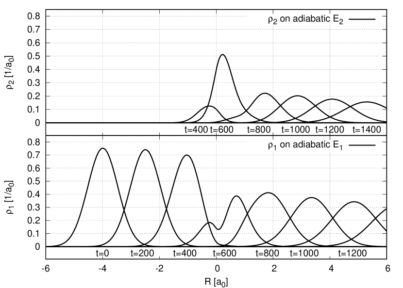
(a)

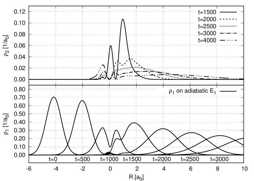
(b)

Figure 5: Time evolution of probability distributions on adiabatic energy surfaces, simple avoided crossing; (a) high momentum Gaussian wavepacket $k=15$ a.u.; (b) low momentum Gaussian wavepacket $k=8.5$ a.u.

(a)

(b)

Figure 6: Transmission and reflection probabilities as function of time in simple avoided crossing; (a) high momentum Gaussian wavepacket $k=15$ a.u.; (b) low momentum Gaussian wavepacket $k=8.5$ a.u.

Figure 5 shows the time evolution of the probability distributions (squared amplitude of the wavefunction $\left|\psi(R,t)\right|^{2}$) on each of the adiabatic electronic surfaces. And Fig. 6 shows the transmission and reflection probabilities (integrals for $R>0$ and $R<0$) evolving over time.

In the high momentum case (Fig. 5a) the packet has enough energy to put about 32% of the population on the upper energy surface. Entering higher level $E_{2}(R)$ caused the wave packet to lose energy, it has smaller momentum and is propagating slower as can be seen by the time labels put beneath the center of each packet in the Fig. 5a. Figure 6a shows the transmission and reflection probabilities for high momentum case. It can be seen that whole packet passes through the crossing point and reflection vanishes over time. The final population is about twice higher on the lower electronic surface than on the upper one.

In the low momentum case (Fig. 5b) the packet doesn’t have enough energy to populate the higher energy surface. Note the vertical scale on the upper level $\rho_{2}$ in Fig. 5b. After going up, the packet almost does not move forward and instead it is leaking back to the lower level in both directions. It can be seen in Fig. 6b that the reflection weakly increases over time while transmission on both electronic surfaces slowly decreases. Most (91%) of the final population resides on the lower surface.

The obtained results are in very good agreement with [58, 59]. Please note that I obtained these results using a different, arguably more precise, time integration algorithm than the one used in [58, 59]. Also see Section 5.2.3 for precision and performance comparison of these calculations against the global Chebyshev propagator [16, 17].

5.2.2 Dual avoided crossing

(a)

(b)

Figure 7: Model surfaces potential matrix of the dual avoided crossing example; (a) diabatic representation; (b) adiabatic representation, $D_{12}$ is the nonadiabatic coupling element (it is drawn as divided by 12 because the coupling is large).

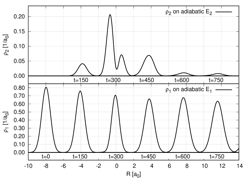
(a)

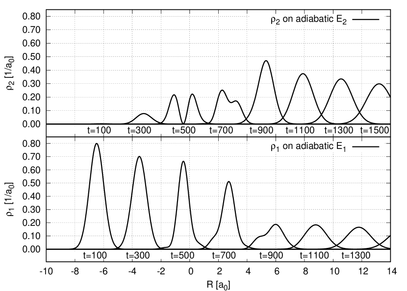
(b)

Figure 8: Time evolution of probability distributions on adiabatic energy surfaces, dual avoided crossing; (a) high momentum Gaussian wavepacket $k=52$ a.u.; (b) low momentum Gaussian wavepacket $k=30$ a.u.

(a)

(b)

Figure 9: Transmission and reflection probabilities as function of time in dual avoided crossing; (a) high momentum Gaussian wavepacket $k=52$ a.u.; (b) low momentum Gaussian wavepacket $k=30$ a.u.

In the second standard benchmark [58, 59] the potential matrix elements in diabatic representation $V_{ij}(R)$ are defined as follows (Fig. 7a):

$$\begin{split}V_{11}(R)&=0\\ V_{22}(R)&=-Ae^{-BR^{2}}+E_{0}\\ V_{12}(R)&=V_{21}(R)=Ce^{-DR^{2}}\end{split}$$ (40)

with the parameters assuming values: $A=0.1$, $B=0.28$, $C=0.015$, $D=0.06$ and ${E_{0}=0.05}$. In this example the diabatic potentials cross each other twice and a wide Gaussian off-diagonal potential is assumed. The adiabatic surfaces exhibit two avoided crossings (Fig. 7b) and the nonadiabatic coupling element $D_{12}$ (Eq. 35) has two pronounced peaks.

The time evolution of probability distributions is shown on Fig. 8 and respective transmission and reflection probabilities are on Fig. 9.

The high momentum case in Fig. 8a demonstrates the effect of destructive interference between the first and second crossing. The wave packet populates the higher level around $t=150$ ($\rho_{2}$ in Fig. 8a) then peaks at around $t=350$ (transmission 2 in Fig. 9a) and arrives to second crossing at about the same phase at which it entered the higher level, but this time the nonadiabatic coupling element $D_{12}(R)$ (Fig. 7b) has negative sign. Same phase of packet in conjunction with negative sign of $D_{12}(R)$ causes the wave packet to leave the higher electronic surface almost completely, despite having high momentum. This effect can be seen in Fig. 9a, where in the end about 98% of population resides on the lower energy surface.

The low momentum case (Fig. 8b) shows constructive interference. First at around $t=500$ about 32% of the population enters the higher energy surface ($\rho_{2}$ in Fig. 8b), then at second crossing additional 32% enters $\rho_{2}$. At $t=900$ there is a significant population increase. Figure 9b shows that about 64% of the population was transmitted to the higher energy surface. This phenomenon is also known as Stükelberg oscillations and occurs when the time spent by the wave packet between two coupling regions is an integer or half integer multiple of mean wavepacket oscillations.

Again, the obtained results are in very good agreement with [58, 59].

5.2.3 Precision and speed tests

Table 5: Precision test of results from semi-global propagator compared against itself, but with higher computation precision. Error is given in terms of ULP (see footnote¹), where the size of ULP for each row is given in the last column (its precise value is in Table 4). There is no row for boost float128 because there is no result with higher precision against which it can be compared, hence it is used only as reference against which lower precision results are compared.

Benchmark type	Precision	long double	boost float128	ULP size
single crossing	double	6	6	$2.2\times 10^{-16}$
high $k_{0}$	long double	—	10	$1.1\times 10^{-19}$
single crossing	double	14	14	$2.2\times 10^{-16}$
low $k_{0}$	long double	—	23	$1.1\times 10^{-19}$
dual crossing	double	14	14	$2.2\times 10^{-16}$
high $k_{0}$	long double	—	126	$1.1\times 10^{-19}$
dual crossing	double	7	7	$2.2\times 10^{-16}$
low $k_{0}$	long double	—	110	$1.1\times 10^{-19}$

Table 6: Precision test of results from semi-global propagator (rows in the table) compared against results from global Chebyshev propagator [16] (columns in the table). Error is given in terms of ULP¹. The size of ULP for each row is given in the last column (its precise value is in Table 4).

	semi-global	global Chebyshev propagator [16]
Benchmark type	Precision	double	long double	boost float128	ULP size
single crossing	double	142	5	6	$2.2\times 10^{-16}$
high $k_{0}$	long double	—	3822	10	$1.1\times 10^{-19}$
	boost float128	—	—	548 / 2164‡	$1.9\times 10^{-34}$
single crossing	double	133	13	14	$2.2\times 10^{-16}$
low $k_{0}$	long double	—	1023	23	$1.1\times 10^{-19}$
	boost float128	—	—	2433 / 7494‡	$1.9\times 10^{-34}$
dual crossing	double	136	9	14	$2.2\times 10^{-16}$
high $k_{0}$	long double	—	15700	126	$1.1\times 10^{-19}$
	boost float128	—	—	1922	$1.9\times 10^{-34}$
dual crossing	double	745	17	7	$2.2\times 10^{-16}$
low $k_{0}$	long double	—	20237	110	$1.1\times 10^{-19}$
	boost float128	—	—	3416	$1.9\times 10^{-34}$

 
^‡ Smaller ULP error value is with the number of elements in the series of the global Chebyshev propagator [16, 17] equal to $10\,R$, larger ULP error is with $1.3\,R$, see footnote²³ for details. Interestingly $1.3\,R$ was enough for float128 in dual crossing calculations.

The calculations from two previous sections (single and dual avoided crossings) are used in this section to compare the precision and performance with the global Chebyshev propagator [16, 17]. This section will also demonstrate the speed gain obtained by using the semi-global propagator.

The parameters of semi-global method used in this comparison are shown in Table 4. The $M$ parameter can be very low because there is no time-dependence in the Hamiltonian, the $K$ parameter was adjusted to be the minimal value of $K$ where the warning about too small $K$ is not printed (see Listing 1, line 48). Namely the estimated error of the function of the matrix is smaller than $\varepsilon$. The $\varepsilon$ parameter is set to the ULP error because maximum possible precision in the calculations is used here. And the timestep used is $\Delta t=1$ a.u.

The global Chebyshev propagator [16, 17] has only one parameter, namely how many elements in the series are calculated, and its value is actually fixed by the design of the algorithm to be $1.3\,R$ (this recommendation is given in [17]), where $R=\frac{\Delta t}{2\hbar}\left({E}_{max}-{E}_{min}\right)$. This value was found to provide full precision in nearly all of the calculations, even for higher precision types.

To compare the two algorithms I am performing the same calculation of transmission and reflection probabilities for all four cases (Table 4 and Figures 6 and 9) using both semi-global method and the global Chebyshev propagator [16, 17]. The results of transmission and reflection probabilities are stored in a text file with all significant digits (column 2 in Table 8). Since the timestep $\Delta t=1$ a.u. and because the transmission and reflection probabilities are stored for each timestep the text files contain the number of lines equal to the total simulation duration (”simulation time” in Table 4) for each of the four cases. These numbers are then compared against the reference result and the maximum error in terms of the units of ULP found for each case is given in Tables 4-6.

The Table 4 shows the results of comparison of the global Chebyshev propagator [16, 17] with itself but with higher numerical precision. The largest error found is for dual crossing, low momentum when comparing long double with float128 precision and equals to 20242 ULP units (where each ULP in this case equals to $1.1\times 10^{-19}$). All ULP errors where a comparison is done between long double and float128 are unusually high and they can be explained by the following phenomenon: several of the last elements in the series of the Chebyshev propagator are very small since the Bessel function values are decaying exponentially, this results in addition of very small values to an otherwise large values resulting from the previous elements in the series. Hence the contribution of the last elements in the series vanishes and produces a slightly less accurate result than would be possible if higher precision was used. Very similar ULP error values will appear again in Table 6.

The Table 6 shows the results of comparison of semi-global method against itself, but with higher precision. The largest error is 126 ULP units (where each ULP in this case equals to $1.1\times 10^{-19}$) and is significantly smaller than in Table 4 which means that the semi-global algorithm overall has higher accuracy than the global Chebyshev propagator.

Finally the Table 6 shows the comparison of semi-global algorithm against the global Chebyshev propagator. In this case it is also possible to compare results for float128 precision between the two algorithms. The largest ULP error is 20237 for the comparison between long double semi-global and long double global Chebyshev propagator. This value is almost equal to the largest ULP error found in Table 4 and indicates that indeed the global Chebyshev propagator has lower accuracy. The comparison between float128 types of both methods is more favorable with largest ULP error equal to 3416 or 7494 if $1.3\,R$ elements in the series are used in the global Chebyshev propagator.

All the calculations discussed in previous paragraphs took a certain amount of time which was measured to test the computation speed of both algorithms. These results are summarized in Table 8 separately for each precision, averaged over the four simulation cases. The semi-global method turns out to be $1.9\times$ faster than the global Chebyshev propagator for double precision and even faster for higher precisions.

I would like to point out that the global Chebyshev propagator [16, 17] is commonly used to validate accuracy of other time propagation methods [64], while in my precision and speed test it turned out to perform worse than semi-global method in both precision and the calculation speed.

The tests discussed in this section are available in the folder Section_5.2.3_PrecisionTest in the supplementary materials.

6 Benchmarks of high precision quantum dynamics

As mentioned in Section 3, I would like to emphasize that this algorithm is implemented in C++ for arbitrary floating point precision types, specified during compilation. It works just as well for types with 15, 18 or 33 decimal places. This is the reason why Real type instead of double is used e.g. in line 5 in Listing 1. The Real type is set during compilation to one of the following types: double, long double or float128. The list of all high precision types, the number of decimal places and their speed relative to double is given in Table 8. It follows my work on high precision in YADE, a software for classical dynamics calculations [56]. However the arbitrary precision types boost mpfr and boost cpp_bin_float are currently not available in the quantum dynamics code because the Fast Fourier Transform (FFT) routines for them are currently unavailable in the Boost libraries [65]. To resolve this problem I took part in the Google Summer of Code 2021 [66] as a mentor and now the high precision FFT code is in preparations to be included in the Boost libraries. The report from high precision FFT implementation in Boost is available here [67]. After that work is complete all types listed in Table 8 will be available for quantum dynamics calculations.

Table 7: Performance comparison of semi-global propagator against global Chebyshev propagator [16]. Values are averaged over all four benchmark types. The semi-global propagator is significantly faster than global Chebyshev propagator.

	computation speed of semi-global propagator
Precision	compared to global Chebyshev propagator [16]
double	$1.9\times$ faster
long double	$21.9\times$ faster
boost float128	$8.1\times$ faster

Table 8: The high-precision benchmark: comparison between classical dynamics [56] and quantum dynamics. The speed is shown as relative to speed at double precision

	Decimal	Classical dynamics	Quantum dynamics
Precision	places	speed w.r.t double [56]	speed w.r.t double
float	6	$1.01\times$ faster
double	15	—	—, $\varepsilon=2.2\times 10^{-16}$
long double	18	$1.4\times$ slower	$3.5\times$ slower, $\varepsilon=1.1\times 10^{-19}$
boost float128	33	$4.7\times$ slower	$50\times$ slower, $\varepsilon=2.2\times 10^{-16}$
boost float128	33		$170\times$ slower, $\varepsilon=1.9\times 10^{-34}$
boost mpfr†	62	$13.5\times$ slower
boost mpfr	150	$19.1\times$ slower
boost cpp_bin_float	62	$24.2\times$ slower

 
^† for future comparison with libqd-dev library.

Table 8 shows the speed comparison between different high-precision types, relative to double, separately for classical dynamics and quantum dynamics. The classical dynamics are reproduced from YADE benchmark [56] to serve as a reference. I have done the quantum dynamics benchmark using the example of atom in an intense laser field from previous Section 5.1. I used the same parameters with the exception of changing $\varepsilon$ (Eq. 27) to match the ULP error of selected precision as provided in table.

The long double precision in quantum dynamics is about $3.5\times$ slower and in exchange provides about $2000$ times greater precision. This might be useful in some situations for quick verification of results.

For the float128 type I did the benchmark twice, first for the $\varepsilon$ same as for double type, then for the significantly smaller $\varepsilon$ matching the float128 type. We can see that using $\varepsilon=2\times 10^{-16}$ from double for the float128 makes it about $50\times$ slower. When using full float128 precision then the decreased error tolerance $\varepsilon$ forces more iterations in Eq. 28 consequently making it $170\times$ slower. If one wished to calculate with larger tolerance, say $\varepsilon=1\times 10^{-25}$, then still float128 has to be used, and it will have speed somewhere between the two values in Tab. 8.

I would like to mention that from my experience [57], it is better to increase $\Delta t$ and allow more sub-iterations in Equation 28 as it speeds up calculation more than changing the $K$ and $M$ parameters. For example, this atom in the laser field calculation took 30 seconds with double and $\Delta t=0.1$ a.u. and 10 minutes with double and $\Delta t=0.0041(6)$ a.u. both having the same $\varepsilon=2\times 10^{-16}$ error tolerance.

Moreover, the original code [2], which deals with a single Schrödinger equation, was written in Matlab [68] and the same simulation which took me 30 seconds in C++, took about 5 minutes in Octave. So the $10\times$ speed gain due to migrating from Octave to C++ can now be wisely spent on higher precision calculations or on simulating larger systems.

7 Accompanying C++ source code package

The C++ source code has been run and tested on Linux Ubuntu, Debian and Devuan, and it should run without significant tweaks on any modern GNU/Linux operating system. Some tweaks might be needed for other operating systems such as MacOS or Windows. In general the source code is very minimal in the sense that there is only the implemented semi-global algorithm in files SemiGlobal.hpp and SemiGlobal.cpp together with the tests listed in Section 5 which can be invoked by various makefile calls (see makefile for full list), such as make plot_Coker or make plot_Atom.

All available make targets can be readily found by reading the comments inside the makefile. One notable target is make testAllFast which does almost all the tests and takes about 20 minutes. The full test make testAll takes about 7 hours, due to float128 precision being significantly slower. From all implemented tests, the file test_single_dual_crossing.cpp is the most interesting because it contains code for working with multiple electronic levels as well as the placeholder code for time dependence in the potential (although it is not used). It is this source code with a generic Hamiltonian calc_Hpsi (Listing 2) which is discussed in Section 4. Other test files test_source_term.cpp and test_atom_laser_ABC.cpp are the direct translations of Matlab/Octave code from [2].

The library dependencies are following: libfftw3-dev [70] (version $\geq$ 3.3.8), libboost-all-dev [65] (version $\geq$ 1.71.0) and libeigen3-dev [71] (version $\geq$ 3.3.7-2).

See file README.pdf in the accompanying source code package for additional details about how to use the semi-global algorithm with custom Hamiltonian in custom coordinate representation, such as curvilinear coordinates. The section Usage in the README.pdf will be maintained and improved as questions arise from users.

The SemiGlobal.hpp and SemiGlobal.cpp files are written to be self contained in a generic way adhering to C++ coding standards. This means that these files are readily available to use in other C++ projects with only minimal changes at the interface to “glue” the code to a different codebase. Depending on whether high precision calculations are required in the other software package the file Real.hpp might be used as well.

8 Conclusions

In this paper, I present an implementation of the semi-global algorithm for coupled Schrödinger equations with the time-dependent Hamiltonian and nonlinear inhomogeneous source term as a means to describe the time-dependent processes in femto- and attosecond chemistry. The code works for multiple coupled electronic states and supports high precision computations with types long double (18 decimal places) and float128 (33 decimal places). Higher arbitrary precision types will become available in the future once FFT algorithm for them becomes ready to use in the C++ boost library.

The semi-global algorithm is verified to work correctly by comparing its results with five reference solutions: (1) atom in an intense laser field (2) single avoided crossing (3) dual avoided crossing (4) Gaussian packet in a forced harmonic oscillator and (5) forced harmonic oscillator with an inhomogeneous source term. All of them are available in the accompanying source code package.

The precision and performance test revealed that the semi-global algorithm is more accurate than the global Chebyshev propagator, while being about two times faster for double precision and even faster for higher precisions.

This C++ code, which is $10\times$ faster than the original Matlab/Octave code upon which it was based, can be used to produce reference high accuracy solutions of various problems such as: nonlinear problems, problems with inhomogeneous source term, mean field approximation, Gross-Pitaevskii approximation or scattering problems.

The attached C++ source code is self contained which makes it possible to reuse the algorithm in different software packages.

Supplementary materials

This paper is accompanied by a file SemiGlobalCpp.zip which contains the C++ source code for GNU/Linux described above, licensed under the GNU GPL v.2 license.

Author Information

Corresponding Author
* E-mail: jkozicki@pg.edu.pl
ORCID
Janek Kozicki: 0000-0002-8427-7263
Conflicts of interest
There are no conflicts of interest to declare.

References

-
[1]
M. Ndong, H. Tal-Ezer, R. Kosloff, C. P. Koch,
A Chebychev propagator with
iterative time ordering for explicitly time-dependent Hamiltonians, The
Journal of Chemical Physics 132 (6) (2010) 064105.
doi:10.1063/1.3312531.
URL http://dx.doi.org/10.1063/1.3312531 -
[2]
I. Schaefer, H. Tal-Ezer, R. Kosloff,
Semi-global approach for
propagation of the time-dependent schrödinger equation for time-dependent
and nonlinear problems, Journal of Computational Physics 343 (2017)
368–413.
doi:10.1016/j.jcp.2017.04.017.
URL http://dx.doi.org/10.1016/j.jcp.2017.04.017 -
[3]
I. Schaefer, H. Tal-Ezer, R. Kosloff,
Corrigendum to
“semi-global approach for propagation of the time-dependent schrödinger
equation for time-dependent and nonlinear problems” [j. comput. phys. 343
(2017) 368–413] (Aug 2022).
doi:10.1016/j.jcp.2022.111300.
URL http://dx.doi.org/10.1016/j.jcp.2022.111300 - [4] W. Kahan, How Futile are Mindless Assessments of Roundoff in Floating-Point Computation?, https://people.eecs.berkeley.edu/~wkahan/Mindless.pdf (2006).
-
[5]
W. Bao, D. Jaksch, P. A. Markowich,
Numerical
solution of the gross–pitaevskii equation for bose–einstein
condensation, Journal of Computational Physics 187 (1) (2003) 318–342.
doi:10.1016/S0021-9991(03)00102-5.
URL https://www.sciencedirect.com/science/article/pii/S0021999103001025 - [6] N. Balakrishnan, C. Kalyanaraman, N. Sathyamurthy, Time–dependent quantum mechanical approach to reactive scattering and related processes, Physics Reports 280 (1997) 79–144.
-
[7]
M. Beck, The
multiconfiguration time-dependent hartree (mctdh) method: a highly efficient
algorithm for propagating wavepackets, Physics Reports 324 (1) (2000)
1–105.
doi:10.1016/s0370-1573(99)00047-2.
URL http://dx.doi.org/10.1016/S0370-1573(99)00047-2 -
[8]
K. C. Kulander,
Time-dependent hartree-fock
theory of multiphoton ionization: Helium, Physical Review A 36 (6) (1987)
2726–2738.
doi:10.1103/physreva.36.2726.
URL http://dx.doi.org/10.1103/PhysRevA.36.2726 -
[9]
U. Manthe, The multi-configurational
time-dependent hartree approach revisited, The Journal of Chemical Physics
142 (24) (2015) 244109.
doi:10.1063/1.4922889.
URL http://dx.doi.org/10.1063/1.4922889 -
[10]
E. Runge, E. K. U. Gross,
Density-functional theory
for time-dependent systems, Physical Review Letters 52 (12) (1984)
997–1000.
doi:10.1103/physrevlett.52.997.
URL http://dx.doi.org/10.1103/PhysRevLett.52.997 -
[11]
A. Castro, H. Appel, M. Oliveira, C. A. Rozzi, X. Andrade, F. Lorenzen,
M. A. L. Marques, E. K. U. Gross, A. Rubio,
octopus: a tool for the
application of time-dependent density functional theory, physica status
solidi (b) 243 (11) (2006) 2465–2488.
doi:10.1002/pssb.200642067.
URL http://dx.doi.org/10.1002/pssb.200642067 -
[12]
A. D. Becke, Perspective: Fifty
years of density-functional theory in chemical physics, The Journal of
Chemical Physics 140 (18) (2014) 18A301.
doi:10.1063/1.4869598.
URL http://dx.doi.org/10.1063/1.4869598 -
[13]
E. Gross, W. Kohn,
Time-dependent
density-functional theory, Advances in Quantum Chemistry (1990)
255–291doi:10.1016/s0065-3276(08)60600-0.
URL http://dx.doi.org/10.1016/S0065-3276(08)60600-0 - [14] D. Neuhauser, M. Baer, The application of wave packets to reactive atom–diatom systems: a new approach, The Journal of chemical physics 91 (8) (1989) 4651–4657.
- [15] H. Tal-Ezer, R. Kosloff, I. Schaefer, New, highly accurate propagator for the linear and nonlinear schrödinger equation, Journal of Scientific Computing 53 (1) (2012) 211–221.
-
[16]
H. Tal‐Ezer, R. Kosloff, An
accurate and efficient scheme for propagating the time dependent Schrödinger
equation, The Journal of Chemical Physics 81 (9) (1984) 3967–3971.
doi:10.1063/1.448136.
URL http://dx.doi.org/10.1063/1.448136 - [17] R. Kosloff, Quantum molecular dynamics on grids, Department of Physical Chemistry and the Fritz Haber Research Center (1997).
-
[18]
W. Magnus,
On the
exponential solution of differential equations for a linear operator,
Communications on Pure and Applied Mathematics 7 (4) (1954) 649–673.
arXiv:https://onlinelibrary.wiley.com/doi/pdf/10.1002/cpa.3160070404,
doi:10.1002/cpa.3160070404.
URL https://onlinelibrary.wiley.com/doi/abs/10.1002/cpa.3160070404 - [19] Z. Sun, W. Yang, D. H. Zhang, Higher-order split operator schemes for solving the schrödinger equation in the time-dependent wave packet method: applications to triatomic reactive scattering calculations, Physical Chemistry Chemical Physics 14 (6) (2012) 1827–1845.
- [20] U. Peskin, R. Kosloff, N. Moiseyev, The solution of the time dependent schrödinger equation by the (t, t’) method: The use of global polynomial propagators for time dependent hamiltonians, The Journal of chemical physics 100 (12) (1994) 8849–8855.
-
[21]
H. Tal-Ezer, On Restart and Error
Estimation for Krylov Approximation of , SIAM Journal on
Scientific Computing 29 (6) (2007) 2426–2441.
doi:10.1137/040617868.
URL http://dx.doi.org/10.1137/040617868 - [22] M. Abramowitz, I. Stegun, Handbook of mathematical functions, Dover publications, inc. New York (reprint), 2013.
-
[23]
H. Tal-Ezer, Polynomial
approximation of functions of matrices and applications (1989).
doi:10.1007/bf01061265.
URL http://dx.doi.org/10.1007/BF01061265 -
[24]
J. Muga, J. Palao, B. Navarro, I. Egusquiza,
Complex absorbing
potentials, Physics Reports 395 (6) (2004) 357–426.
doi:10.1016/j.physrep.2004.03.002.
URL http://dx.doi.org/10.1016/j.physrep.2004.03.002 -
[25]
J. Palao, J. Muga, A
simple construction procedure of absorbing potentials, Chemical Physics
Letters 292 (1–2) (1998) 1–6.
doi:10.1016/s0009-2614(98)00635-6.
URL http://dx.doi.org/10.1016/S0009-2614(98)00635-6 -
[26]
A. Palacios, F. Martín, The quantum
chemistry of attosecond molecular science, WIREs Computational Molecular
Science 10 (1) (2019).
doi:10.1002/wcms.1430.
URL http://dx.doi.org/10.1002/wcms.1430 -
[27]
D. Goldberg, What every computer
scientist should know about floating-point arithmetic, ACM Computing Surveys
23 (1) (1991) 5–48.
doi:10.1145/103162.103163.
URL http://dx.doi.org/10.1145/103162.103163 -
[28]
D. Bailey, R. Barrio, J. Borwein,