Linear Regression on Manifold Structured Data:
the Impact of Extrinsic Geometry on Solutions

Abstract

In this paper, we study linear regression applied to data structured on a manifold. We assume that the data manifold is smooth and is embedded in a Euclidean space, and our objective is to reveal the impact of the data manifold’s extrinsic geometry on the regression. Specifically, we analyze the impact of the manifold’s curvatures (or higher order nonlinearity in the parameterization when the curvatures are locally zero) on the uniqueness of the regression solution. Our findings suggest that the corresponding linear regression does not have a unique solution when the embedded submanifold is flat in some dimensions. Otherwise, the manifold’s curvature (or higher order nonlinearity in the embedding) may contribute significantly, particularly in the solution associated with the normal directions of the manifold. Our findings thus reveal the role of data manifold geometry in ensuring the stability of regression models for out-of-distribution inferences.

1 Introduction

The manifold hypothesis posits that real-world data points typically cluster on a lower-dimensional manifold, denoted as $\mathcal{M}$, within a high-dimensional encoding space like $\mathbb{R}^{d}$. This concept has been investigated in numerous studies (Hein & Maier, 2006; Narayanan & Mitter, 2010; Niyogi et al., 2008; Tenenbaum et al., 2000). Fefferman et al. (2016) established a theoretical and algorithmic framework to statistically validate and test the manifold hypothesis. Other rigorous experiments (Brand, 2002; Ruderman, 1994; Roweis & Saul, 2000; Schölkopf et al., 1998) have also provided empirical evidence supporting the existence of low-dimensional manifold, particularly in the context of image data sets.

The related current mainstream research fields can be classified into the following two categories: (i) Dimensionality reduction methods (Abdi & Williams, 2010; Roweis & Saul, 2000; Tenenbaum et al., 2000); (ii) Approximation theory for deep learning models for functions supported on low-dimensional manifolds (Chen et al., 2019; Cloninger & Klock, 2021; Shaham et al., 2018). One of the objectives of (i) is to reduce the “curse of dimensionality” imposed by the embedding space directly and explicitly by (approximately) encoding the data into a lower dimensional space. In the case of (ii), results show that neural networks can approximate functions that are defined on an embedded smooth manifold with costs depending on the intrinsic dimensions of the manifold itself not the dimensionality of the embedding space. However, these studies use only some global geometric quantities, such as the reach (Federer, 1959) of the data manifold to establish the approximation estimates. Moreover, relatively little is known about the stability of neural networks when evaluating inputs that deviate from the manifold, i.e., inputs that lie outside the training data distribution. Further research is needed to uncover the stability characteristics of neural networks in these situations and extend our knowledge of their performance and limitations.

Instead of studying the dimensionality reduction or approximation techniques when data are concentrated on a low-dimensional manifold, we propose to explicitly explore the influence of extrinsic geometric information of the data manifold on the learning process and outcome. In particular, we study linear regression models under the assumption that the data is distributed on a smooth manifold embedded in a higher dimensional Euclidean space. To unveil the influence of the manifold’s geometry on the regression, we focus our analysis on a localized region around the manifold. We thus refer to linear regression in such a setup as the local linear regression problem. Specifically, we focus on the issues of uniqueness and stability of solutions in the well-posedness of the linear regression, stemming from the local geometry of the data manifold. We further discuss the effect of adding noise as regularization for the local linear regression under the low-dimensional manifold setup.

More precisely, we assume a smooth low-dimensional data manifold $\mathcal{M}$ embedded in $\mathbb{R}^{d}$, and we have the data/target function $g:\mathbb{R}^{d}\to\mathbb{R}$. Local linear regression means that we construct an affine function

$$f(\mathbf{x},\mathbf{w},b)=\mathbf{w}\cdot\mathbf{x}+b,~{}~{}~{}\mathbf{x},\mathbf{w}\in\mathbb{R}^{d},b\in\mathbb{R},$$ (1)

by solving the least square optimization problem

$$\min_{\mathbf{w}\in\mathbb{R}^{d},b\in\mathbb{R}}\mathcal{L}(\mathbf{w},b)=\int_{\Omega}\lvert f(\mathbf{x},\mathbf{w},b)-g(\mathbf{x})\rvert^{2}\rho(\mathbf{x})\mathrm{d}\mathbf{x},$$ (2)

where $\rho(\mathbf{x})$ is the data density in a small neighborhood $\Omega\subset\mathcal{M}$. The local linear regression model is of interest for two primary reasons. On the one hand, the local linear regression model, which is also known as the moving least-square method (Cleveland, 1979; Cleveland & Devlin, 1988; Levin, 1998), is widely studied in computer graphics (Schaefer et al., 2006), numerical analysis (Gross et al., 2020; Liang & Zhao, 2013), and machine learning (Trask et al., 2019; Wang et al., 2010). On the other hand, any deep neural network (DNN) with ReLU activation function is essentially a piece-wise linear function (Arora et al., 2016), which can be interpreted as a different parametrization of the local linear regression model or the linear adaptive finite element method (Babuvska & Rheinboldt, 1978). By further studying the approximation theory of adaptive finite elements and connections between ReLU DNNs and the linear finite element methods (He et al., 2020), one can show that the linear region of the learned ReLU DNN is relatively small if the Hessian of the target function has a lower bound on that region. Consequently, the optimal learned ReLU DNN should comprise multiple local linear regressions within small linear regions if the Hessian of the target function is not small. In addition to these, a general regression model $f(\mathbf{x};\theta)=\mathbf{w}\cdot\psi(\mathbf{x};\tilde{\theta})+b$ with feature map $\psi(\mathbf{x};\tilde{\theta})$ can be understood as a linear regression on the latent manifold $\psi\left(\mathcal{M}\right):=\{\psi(\mathbf{x};\tilde{\theta})\,:\,\mathbf{x}\in\mathcal{M}\}$. Therefore, studying how the geometric information of the manifold affects the linear regression system can benefit us in understanding the general regression model or regularizing the feature map (Zhu et al., 2018).

Moreover, it is important to consider that datasets in practice often contain noise. Thus, it is imperative to delve into the impact of noises on the linear regression solution. As studied in (He et al., 2023), noise in the codimension of the data manifold can provide a regularization that improves the stability of linear or ReLU DNN regressions. In this work, we further showcase how the presence of noise can potentially prevent the degeneracy and provide regularization effects for the linear regression model when the embedded data manifold is not flat.

To summarize, in this study, we focus on local linear regression models with data on low-dimensional submanifolds embedded in a Euclidean space and mainly investigate the following questions:

1. How the uniqueness of solutions for the local linear regression problem is dependent on the local geometric information, such as curvatures, of the data manifold;

2. How the local geometric information affects the regression outcomes;

3. How noises interact with the local geometric information of the data manifold and affect learning.

Other related work

Linear dimension reduction, manifold learning, and the intrinsic dimensionality of data and features.

A multitude of dimensionality reduction methods exists, both in the supervised and unsupervised settings, including Linear Discriminant Analysis (LDA) (Balakrishnama & Ganapathiraju, 1998), Principal Component Analysis (PCA) (Abdi & Williams, 2010), Multiple Dimensional Scaling (MDS) (Cox & Cox, 2008), and Canonical Correlation Analysis (CCA) (Hardoon et al., 2004). The random projection framework provides a theoretical justification for data compression (Bourgain et al., 2011; Johnson & Lindenstrauss, 1984; Krahmer & Ward, 2011) using random matrices and sampling methods. Manifold learning algorithms (Belkin & Niyogi, 2003; Brand, 2002; Chui & Mhaskar, 2018; Donoho & Grimes, 2003; Roweis & Saul, 2000; Saul & Roweis, 2003; Tenenbaum et al., 2000; Weinberger et al., 2004), as a direct result of low-dimensional manifold hypothesis, aims at finding local low dimensional representations of the high dimensional data. In the context of deep learning, Gong et al. (2019) finds the intrinsic dimensionality of deep neural network representations is significantly lower than the dimensionality of the embedded space of data. Across layers of neural networks, Ansuini et al. (2019) further showcases that the intrinsic dimension of features first increases and then progressively decreases in the final layers. Pope et al. (2021) investigates the role of low-dimensional structure in deep learning by applying dimension estimation tools to natural image datasets. They find that neural networks could learn and generalize better on low-dimensional datasets.

Approximation of functions supported on a manifold.

Several studies have shown that the approximation rate for functions defined on low-dimensional manifolds is determined by the intrinsic dimensions of the manifolds rather than the dimensions of the ambient spaces. Shaham et al. (Shaham et al., 2018) achieves this rate by utilizing the wavelet structure to construct a sparsely-connected neural network. Chen et al. (2019) and Schmidt (2019) implement chart determination (or partition of unity) and Taylor approximation with ReLU neural network to get the results. Liu et al. (2021) obtains similar approximation rates for approximating Besov functions with convolutional residual networks. As for stability, a more comprehensive understanding requires making specific assumptions about the form of the functions being approximated. For instance, Cloinger et al. (2021) explored the case where functions are locally constant along the normals of the manifold.

The impact of the data manifold in learning.

The exploration of how the geometry of the data manifold affects the learning process and how to utilize this information to enhance learning outcomes has received limited attention in the existing literature. For deep linear and ReLU neural networks, He et al. (2023) investigates the variation of the learned functions in the direction transversal to a linear subspace where the training data is distributed. This work also delves into the side effects and regularization properties of network depth and noise within the codimension of the data manifold. Following the low-dimensional manifold hypothesis, Zhu et al. (2018) proposes to apply the dimensionality of the data manifold as a regularizer in deep neural networks to achieve better performance for image classification. Furthermore, Dong et al. (2020) uses the curvature information as the regularizer for missing data recovery tasks.

2 Local linear regression on embedded manifolds

Denote $\mathbf{x}=(x_{1},x_{2},\cdots,x_{d})$ and $\mathbf{w}=(w_{1},w_{2},\cdots,w_{d})$. The solution to the linear regression problem (1)-(2) should satisfy the following $(d+1)\times(d+1)$ linear system, which is also known as the least square problem:

$$\begin{bmatrix}\langle x_{1}^{2}\rangle&\langle x_{1}x_{2}\rangle&\dots&\langle x_{1}x_{d}\rangle&\langle x_{1}\rangle\\ \langle x_{1}x_{2}\rangle&\langle x_{2}^{2}\rangle&\dots&\langle x_{2}x_{d}\rangle&\langle x_{2}\rangle\\ \vdots&\quad&\ddots&\quad&\vdots\\ \langle x_{1}x_{d}\rangle&\langle x_{2}x_{d}\rangle&\dots&\langle x_{d}^{2}\rangle&\langle x_{d}\rangle\\ \langle x_{1}\rangle&\langle x_{2}\rangle&\dots&\langle x_{d}\rangle&1\end{bmatrix}\begin{bmatrix}w_{1}\\ w_{2}\\ \vdots\\ w_{d}\\ b\end{bmatrix}=\begin{bmatrix}\langle gx_{1}\rangle\\ \langle gx_{2}\rangle\\ \vdots\\ \langle gx_{d}\rangle\\ \langle g\rangle\end{bmatrix},$$ (3)

where the $\langle\,\boldsymbol{\cdot}\,\rangle$ notation denotes averaging with the density $\rho(\mathbf{x})$:

$$\langle\,\boldsymbol{\cdot}\,\rangle=\int_{\Omega}\;\boldsymbol{\cdot}\;\rho(\mathbf{x})\mathrm{d}\mathbf{x}.$$

We say that the linear regression problem (1)-(2) is ill-posed when (3) does not have a unique solution.

When the scope of the linear regression is restricted to a local subset of the data manifold $\mathcal{M}$, the corresponding analysis can be simplified through a suitable change of coordinates given by a unitary transformation followed by a translation. The following simple lemma shows that this change of coordinates preserves the equivariance of the linear regression problem (1)-(2).

Lemma 2.1.

Let $Q\in\mathbb{R}^{d\times d}$ be an orthogonal matrix and $\mathbf{t}_{0}\in\mathbb{R}^{d}.$ If $(\mathbf{w^{*}},b^{*})\in\mathbb{R}^{d}\times\mathbb{R}$ minimizes

$$\mathcal{L}(\mathbf{w},b):=\int_{\Omega}\lvert(\mathbf{x}\cdot\mathbf{w}+b)-g(\mathbf{x})\rvert^{2}\rho(\mathbf{x})\mathrm{d}\mathbf{x}$$

then $(Q\mathbf{w}^{*},\,b^{*}-(Q\mathbf{w}^{*})\cdot\mathbf{t}_{0})$ minimizes

$$\tilde{\mathcal{L}}(\mathbf{w},b):=\int_{\Omega}\lvert(Q\mathbf{x}+\mathbf{t}_{0})\cdot\mathbf{w}+b-g(\mathbf{x})\rvert^{2}\rho(\mathbf{x})\mathrm{d}\mathbf{x}$$

Proof.

Define the affine transformation $\phi(\mathbf{x})=Q\mathbf{x}+\mathbf{t}_{0}$ and denote $\widetilde{\mathbf{x}}=\phi(\mathbf{x})$ and $\tilde{\Omega}$ be the image of $\Omega$ under this affine transformation. Since $Q$ is orthogonal and has full rank, $\phi$ is a change of coordinates. Let $\widetilde{\mathbf{w}}=(\widetilde{w}_{1},\,\widetilde{w}_{2},\,\dots,\,\widetilde{w}_{d-1},\,\widetilde{w}_{y})$ and $\widetilde{b}$ be the new set of parameters for the linear regression problem in the transformed domain. Further define $\widetilde{g}(\widetilde{\mathbf{x}})=g\big{(}Q^{T}(\widetilde{\mathbf{x}}-\mathbf{t}_{0})\big{)}$ so that $\tilde{g}\big{(}\phi(\mathbf{x})\big{)}=g(\mathbf{x})$, and similarly $\tilde{\rho}$.

$$\min_{\widetilde{\mathbf{w}},\tilde{b}}\mathcal{L}(\widetilde{\mathbf{w}},\,\widetilde{b})=\min_{\widetilde{\mathbf{w}},\widetilde{b}}\int_{\widetilde{\Omega}}\lvert\widetilde{\mathbf{w}}^{T}\widetilde{\mathbf{x}}-\tilde{g}(\widetilde{\mathbf{x}})\rvert^{2}\tilde{\rho}(\widetilde{\mathbf{x}})\mathrm{d}\tilde{\mathbf{x}}$$

$$= \min_{\widetilde{\mathbf{w}},\widetilde{b}}\int_{\Omega}\lvert\widetilde{\mathbf{w}}^{T}\mathbf{t}_{0}+\widetilde{\mathbf{w}}^{T}Q\mathbf{x}+\widetilde{b}-g(\mathbf{x})\rvert^{2}\rho({\mathbf{x}})|det(Q)|\mathrm{d}\mathbf{x}$$

$$= \min_{\mathbf{w},b}\int_{\Omega}\lvert\mathbf{w}^{T}\mathbf{x}+b-g(\mathbf{x})\rvert^{2}\rho({\mathbf{x}})\mathrm{d}\mathbf{x}=\min_{\mathbf{w},b}\mathcal{L}(\mathbf{w},\,b).$$

Above, we use the fact that $|det(Q)|=1$ since $Q$ is orthogonal. Therefore, the equivalence between the minimization problems implies the minimizer of the transformed problem $\{\widetilde{\mathbf{w}},\tilde{b}\}$ can be identified with that of the original problem $\{\mathbf{w},b\}$ through the following bijection: $\mathbf{w}^{T}=\widetilde{\mathbf{w}}^{T}Q,\;b=\widetilde{\mathbf{w}}^{T}\mathbf{t}_{0}+\tilde{b}.$ ∎

So, without loss of generality, we study the least square problem under a suitable local coordinate system, which can facilitate the following queries related to local linear regression on embedded submanifolds.

1. Examining the solvability of (3);

2. Deriving explicit solution formulas;

3. Describing the effect of the data manifold’s geometry on local linear regression more lucidly.

Finally, we outline the assumptions and conventions that will be employed throughout the rest of this work.

Assumptions 2.1.

We have the following assumptions for the data and model with a visual provided in Figure 1 to help demonstrate some of the assumptions:

1. The given data is a local subset of the smooth data manifold $\mathcal{M}\cap U$ with $U\subset\mathbb{R}^{d}$ centered at $\mathbf{x}_{0}$.

2. The linear regression problem is investigated under a local coordinate frame of $\mathbb{R}^{d}$, where $\mathbf{x}_{0}:=\mathbf{0}$ and the tangent space $\mathcal{T}_{\mathbf{x}_{0}}\mathcal{M}$ at $\mathbf{x}_{0}$ is the independent variable space parameterizing the smooth data manifold locally.

3. The data is uniformly distributed in a subset $\Omega^{\prime}$ of the independent variable space $\mathcal{T}_{\mathbf{x}_{0}}\mathcal{M}$, i.e., $\rho(\mathbf{x})=\frac{1}{\lvert\Omega^{\prime}\rvert}$:

   $$\langle\,\boldsymbol{\cdot}\,\rangle=\frac{1}{\lvert\Omega^{\prime}\rvert}\int_{\Omega^{\prime}}\;\boldsymbol{\cdot}\;\mathrm{d}\mathbf{x}.$$ (4)

4. All the independent variables $x_{i}$ are assumed to be $i.i.d.$ according to $\mathcal{U}\big{(}[-L,L]\big{)}$ where $L\ll 1$ determines the size of the local region $\Omega^{\prime}$.

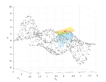
Figure 1: A visualization of a collection of manifold-structured data (the grey point clouds) sampled from a $2$-manifold embedded in $\mathbb{R}^{3}$; the local based point $\mathbf{x}_{0}$ is given by the red dot; the corresponding tangent space $\mathcal{T}_{\mathbf{x}_{0}}\mathcal{M}$ is the yellow plane; the blue surface indicates the part of the submanifold that would be used for local linear regression. Note only the data distribution is shown here, no information of the target function $g$ is presented.

While a more general assumption could be entertained for the data distribution, we contend that the above formulation provides more clarity in the derivations of the linear regression solutions and explicates the primary influence exerted by the local geometry of the underlying manifold.

2.1 Simple curves in $\mathbb{R}^{2}$

We first consider a model problem in which $\mathcal{M}$ is given as the curve $\mathcal{M}:=\big{(}x,y(x)=\kappa x^{2}\big{)}$ in $\mathbb{R}^{2}$ with $\kappa$ characterizes the curvature of $\mathcal{M}$ at $(0,0)$. Since the tangent space at $(0,0)$ is already given as the $x$-axis, A.2 is automatically satisfied. According to A.3-A.4, the local data manifold is given by $\big{(}x,y(x)\big{)}$ where $x\in[-L,L]$ and $\rho(x)=1/2L$. Then, Equation 3 for this model problem becomes the following $3\times 3$ system:

$$\begin{bmatrix}\left<x^{2}\right>&\left<xy\right>&\left<x\right>\\ \left<xy\right>&\left<y^{2}\right>&\left<y\right>\\ \left<x\right>&\left<y\right>&1\end{bmatrix}\begin{bmatrix}w_{x}\\ w_{y}\\ b\end{bmatrix}=\begin{bmatrix}\left<gx\right>\\ \left<gy\right>\\ \left<g\right>\end{bmatrix}.$$ (5)

With A.3-A.4, we have $\left<xy\right>=\left<x\right>=0$, and Equation 3 is further reduced to

$$\begin{bmatrix}\left<x^{2}\right>&0&0\\ 0&\left<y^{2}\right>&\left<y\right>\\ 0&\left<y\right>&1\end{bmatrix}\begin{bmatrix}w_{x}\\ w_{y}\\ b\end{bmatrix}=\begin{bmatrix}\left<gx\right>\\ \left<gy\right>\\ \left<g\right>\end{bmatrix}.$$

The solution is given by

$$\begin{dcases}w_{x}^{*}=\frac{\left<gx\right>}{\left<x^{2}\right>},\\ w_{y}^{*}=\frac{1}{D}(\left<gy\right>-\left<g\right>\left<y\right>),\\ b^{*}=\frac{1}{D}(-\left<y\right>\left<gy\right>+\left<y^{2}\right>\left<g\right>),\end{dcases}$$

where $D$ is the determinant $D:=\left<y^{2}\right>-(\left<y\right>)^{2}$. If $g$ is $C^{2}$:

$$g\big{(}x,\,y(x)\big{)}=g(0)+\frac{\partial g}{\partial x}(0)x+\frac{\partial g}{\partial y}(0)y+\frac{1}{2}\big{(}\frac{\partial^{2}g}{\partial x^{2}}(0)x^{2}+\frac{\partial^{2}g}{\partial xy}(0)xy+\frac{\partial^{2}g}{\partial y^{2}}(0)y^{2}\big{)}+O(|x|^{3}).$$

Combining with $\left<xy\right>=\left<x\right>=0$, we finally have

$$\begin{dcases}w_{x}^{*}=\frac{\partial g}{\partial x}(0)+\mathcal{O}\big{(}L^{2}\big{)},\\ w_{y}^{*}=\frac{\partial g}{\partial y}(0)+\frac{1}{2\kappa}\frac{\partial^{2}g}{\partial x^{2}}(0)+\mathcal{O}\big{(}L^{2}\big{)},\\ b^{*}=g(0)+\mathcal{O}\big{(}L^{4}\big{)},\end{dcases}$$

where the power of $L$ terms are considered to be of higher order since we take $L\ll 1$.

Based on the derived formulas, we observe that the magnitude of $w_{y}^{*}$ tends to blow up when the curvature of the underlying curve $\mathcal{M}$ goes to $0$. To demonstrate this claim, we perform a simple numerical simulation on the linear regression problem with the target function $g(x,y)=2x^{2}+2y^{2}+6xy+3x+4y+10$. We randomly sample $N=1000$ points uniformly in the interval $[-0.1,0.1]$ to obtain $x$, and apply the linear regression solver to fit the data function $g(x,y)$, for different values of the curvature $\kappa$. The simulated result shown in Figure 2 solidifies our assertion: $w_{y}$ tends to blow up as the curvature approaches $0$.

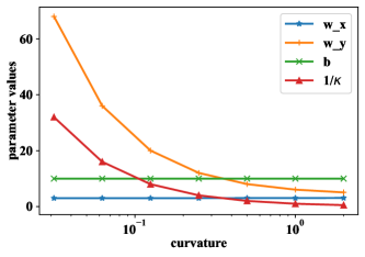
Figure 2: $2$D linear regression solutions on data manifolds $(x,\kappa x^{2})$ with different curvatures $\kappa$. $x$-axis is in log-scale. When curvature is small, the optimal solution $w_{y}^{*}$ is dominated by the curvature effect, in a magnitude related to $\frac{1}{\kappa}$ as we have shown in (2.1).

To summarize, we list the following properties which will persist in more general situations discussed in this paper:

1. The well-posedness of the linear regression.
   The matrix $\begin{bmatrix}\left<y^{2}\right>&\left<y\right>\\ \left<y\right>&1\end{bmatrix}$ will not be invertible if $\left<y^{2}\right>=0$ due to $\kappa=0$. The data manifold is therefore called “flat” at the origin.

2. The effect of geometry on the solutions
   In the case of non-zero curvature, the linear regression problem has a unique solution. However, one must account for the influence of the curvature when attempting to approximate the first-order information of $g$ (unless $g$ is linear). This is particularly relevant when the curvature is small as it could lead to contamination of the target solution. Therefore, the impact of geometry on the solutions in a more general setup should not be overlooked.

2.2 Hypersurfaces in $\mathbb{R}^{d}$

In this section, we derive results similar to those obtained in Section 2.1, which allow us to address the aforementioned inquiries for general hypersurfaces. The hypersurface $\mathcal{M}$ in $\mathbb{R}^{d}$ is an embedded submanifold with codimension $1$. Assume $\mathcal{M}$ is locally smooth ($C^{m}$ for any $m\geq 1$). Then by the inverse function theorem, $\mathcal{M}$ can be locally represented by the graph of a unique continuously differentiable function, meaning there is a smooth mapping $h$ (of full rank) of $(d-1)$ variables defined in the $(d-1)$-dimensional neighborhood $U^{\prime}$ of $\mathbf{x}_{0}$ $s.t.$

$$\mathcal{M}\cap U=\big{\{}x_{d}=y=h(\mathbf{x}^{\prime}):\mathbf{x}^{\prime}\in U^{\prime}\subset\mathbb{R}^{d-1}\big{\}},$$ (6)

where $\mathbf{x}\in\mathbb{R}^{d}=(x_{1},\,x_{2},\,\cdots,\,x_{d})=(\mathbf{x}^{\prime},\,x_{d})$, and $U$ is a neighborhood of $\mathbf{x}_{0}\in\mathbb{R}^{d}$.

Therefore, the tangent space $\mathcal{T}_{\mathbf{x}_{0}}\mathcal{M}$ at $\mathbf{x}_{0}$ is identified by a hyperplane in $\mathbb{R}^{d}$ implying the normal space is only $1$-dimensional since by definition the normal space is spanned by all the unit vectors $\mathbf{n}(\mathbf{x}_{0})$ at $\mathbf{x}_{0}$ that satisfy $\langle\mathbf{n}\,,\,\mathbf{v}\rangle=0$ for all $\mathbf{v}\in\mathcal{T}_{\mathbf{x}_{0}}\mathcal{M}$, where $\langle\cdot\,,\,\cdot\rangle$ is the standard inner product for the embedding space $\mathbb{R}^{d}$. To extend the concept of curvatures from Section 2.1, we can rely on the shape operator (Singer & Thorpe, 2015) from differential geometry:

Proposition 2.2.

The principal curvatures $\kappa_{1},\kappa_{2},\dots,\kappa_{d-1}$ (associated with $\mathbf{n}(\mathbf{x})$) of $\mathcal{M}$ at $\mathbf{x}_{0}$ defined through the shape operator are given by the eigenvalues of the Hessian at $\mathbf{x}_{0}$: $Hess(h)(\mathbf{x}_{0})$ of the graph representation $h$.

Proposition 2.2 establishes a direct relationship between the extrinsic principal curvatures and the Hessian, the generalized second-order derivative, of the graph of $\mathcal{M}$. The following Lemma further motivates and generalizes the surface representation assumed in Section 2.1.

Lemma 2.3.

(Local representation of the hypersurface $\mathcal{M}$)
Locally under a suitable coordinate basis, the hypersurface $\mathcal{M}$ can be approximated by a quadratic form using the principal curvatures up to the second order.

Proof.

The local graph representation of $\mathcal{M}$ is given by $y=h(\mathbf{x}^{\prime})$ for $\mathbf{x}^{\prime}\in U^{\prime}\subset\mathbb{R}^{d-1}$, a neighborhood of $\mathbf{x}^{\prime}_{0}$. Without loss of generality, we take $\mathbf{x}^{\prime}_{0}=\mathbf{0}_{d-1}$. A Taylor expansion of $h$ around $\mathbf{0}_{d-1}$ gives:

$$y=h(\mathbf{x}^{\prime})=h(\mathbf{0}_{d-1})+\nabla h(\mathbf{0}_{d-1})\cdot\mathbf{x}^{\prime}+\frac{1}{2}\mathbf{x}^{\prime T}Hess\big{(}h(\mathbf{0}_{d-1})\big{)}\mathbf{x}^{\prime}+\mathcal{O}(\lVert\mathbf{x}^{\prime}\rVert^{3}).$$

Since $\mathbf{x}=\mathbf{0}\implies h(\mathbf{0}_{d-1})=0$, and $\nabla h(\mathbf{0}_{d-1})=\mathbf{0}_{d-1}$ because $h$ is tangent to the $x$-plane, we have $y=h(\mathbf{x}^{\prime})=\frac{1}{2}\mathbf{x}^{\prime T}Hess\big{(}h(\mathbf{0}_{d-1})\big{)}\mathbf{x}^{\prime}+\mathcal{O}(\lVert\mathbf{x}^{\prime}\rVert^{3})$. The Hessian is semi-positive definite, by diagonalization and a change of basis, we eventually have

$$y=h(\mathbf{x}^{\prime})=\frac{1}{2}\mathbf{x}^{\prime T}\mathcal{K}\mathbf{x}^{\prime}+\mathcal{O}(\lVert\mathbf{x}^{\prime}\rVert^{3}),$$

where $\mathcal{K}$ is a diagonal matrix with its diagonal being the principal curvatures $\kappa_{1},\kappa_{2},\dots,\kappa_{d-1}$ based on Proposition 2.2. Thus $\mathcal{M}$ can be approximated up to the second order by: $y\approx\sum_{i=1}^{d-1}\kappa_{i}x_{i}^{2}.$ ∎

With the above local approximation, we can obtain a local linear regression formula for hypersurface around $\mathbf{x}_{0}$:

Theorem 2.4.

(Solution formulas for local linear regression on hypersurfaces)
When the data manifold $\mathcal{M}$ is a hypersurface with a local approximation $(\mathbf{x}^{\prime},y=\sum_{i=1}^{d-1}\kappa_{i}x_{i}^{2})$ given in Lemma 2.3, under the assumptions A.2-A.4, if the linear regression problem is well-posed, it has the following solution:

$$\begin{dcases}w_{i}*=\frac{\partial g}{\partial x_{i}}(\mathbf{0})+\mathcal{O}(L^{2}),\\ w_{y}^{*}=\frac{\partial g}{\partial y}(\mathbf{0})+\frac{1}{2}\frac{\displaystyle\sum_{i=1}^{d-1}\kappa_{i}\frac{\partial^{2}g}{\partial x_{i}^{2}}(\mathbf{0})}{\displaystyle\sum_{i=1}^{d-1}\kappa_{i}^{2}}+\mathcal{O}(L^{2}),\\ b^{*}=g(\mathbf{0})+\mathcal{O}\Bigg{(}\sum_{i=1}^{d-1}\frac{\partial^{2}g}{\partial x_{i}^{2}}(\mathbf{0})\Big{(}\frac{\displaystyle\sum_{j\neq i}\kappa_{j}^{2}-\kappa_{i}\sum_{j\neq i}\kappa_{j}}{\displaystyle\sum_{k=1}^{d-1}\kappa_{k}^{2}}\Big{)}\frac{L^{2}}{3}\Bigg{)}.\end{dcases}$$

Proof.

Following a similar argument and the same notation introduced in Section 2.1, by symmetry the linear system resulted from the least square minimization is given by:

$$\begin{bmatrix}\langle x_{1}^{2}\rangle&0&&\dots&0&0\\ 0&\langle x_{2}^{2}\rangle&0&\dots&0&0\\ \vdots&\ddots&\ddots&\ddots&\vdots&\vdots\\ 0&0&\dots&0&\langle y^{2}\rangle&\langle y\rangle\\ 0&0&\dots&0&\langle y\rangle&1\end{bmatrix}\begin{bmatrix}w_{1}\\ w_{2}\\ \vdots\\ w_{d-1}\\ w_{y}\\ b\end{bmatrix}=\begin{bmatrix}\langle gx_{1}\rangle\\ \langle gx_{2}\rangle\\ \vdots\\ \langle gx_{d-1}\rangle\\ \langle gy\rangle\\ \langle g\rangle\end{bmatrix}.$$ (7)

Then it is easy to see $w_{i}$ is trivial to obtain, and we again only have a $2\times 2$ system to solve for $w_{y}$ and $b$, similar as in Section 2.1. The rest follows from some algebraic manipulations, see Appendix A for details. ∎

To conclude for the local linear regression on hypersurfaces, we note that we obtain a generalized system with similar structures as in the case of Section 2.1, however, the previous problematic situations become much nicer:

1. The system is invertible as long as we have at least one $\kappa_{i}\neq 0$. When $\kappa_{i}=0$, corresponding higher-order nonlinearity assumes the role of $\kappa_{i}$, meaning the hypersurface only needs to be non-flat in at least one direction.

2. The blow-up effect in $w_{y}^{*}$ caused by curvatures is mitigated: as long as $k_{i}$ is large in some directions, the term $\frac{1}{2}\displaystyle\sum_{i=1}^{d-1}\kappa_{i}\frac{\partial^{2}g}{\partial x_{i}^{2}}(\mathbf{0})/\displaystyle\sum_{i=1}^{d-1}\kappa_{i}^{2}$ would be well-controlled.

2.3 Codimension-$k$ submanifolds

The success of obtaining a solution formula in Section 2.2 is mainly due to the reduction to a $2\times 2$ system in the end of the least square minimization, a direct consequence of the fact that the normal space is always $1$-dimensional for a hypersurface. In general, for a codimension-$k$ submanifold whose normal space is therefore $k$-dimensional, one has to solve a $(k+1)\times(k+1)$ linear system from the least square minimization under the same assumption, hence the solution formula cannot be easily obtained.

Furthermore, from Proposition 2.2 we learn that the diagonalization process and its connection to principal curvatures are strongly predicated on the assumption of maintaining a consistent normal direction. For a $k$-dimensional normal space, there will be one shape operator associated with each orthonormal basis of the normal space, meaning whenever we diagonalize the Hessian of the graph representation along one normal direction and obtain a change of coordinates for the tangent space, the resulting local coordinate frame generally would not diagonalize the others.

To solidify the above statements, consider the example of a $2$-manifold in $\mathbb{R}^{4}$, which is a codimension-$2$ submanifold with $2$ independent normal basis vectors. Following the same procedure as in Section 2.2, we would obtain locally a quadratic graph representation $\big{(}x_{1},x_{2},y_{1}=k_{11}x_{1}^{2}+k_{22}x_{2}^{2}\big{)}$ when restricted on the linear subspace $\mathcal{T}_{\mathbf{x}_{0}}\mathcal{M}\oplus\mathcal{N}_{1}$. With this coordinate frame, locally around $\mathbf{x}_{0}$, $\mathcal{M}$, in general, would take the following form up to some higher order errors:

$$\mathcal{M}_{\mathbf{x}_{0}}=\big{\{}(x_{1},x_{2},y_{1},y_{2})\,\big{|}\,y_{1}=k_{11}x_{1}^{2}+k_{22}x_{2}^{2}+\dots,y_{2}=\tau_{11}x_{1}^{2}+\tau_{12}x_{1}x_{2}+\tau_{22}x_{2}^{2}+\dots\big{\}},$$

where the graph representation along $y_{2}$ is not diagonalized. Besides, after applying local linear regression as in Section 2.2, the resulting linear system from the least square minimization is given as:

$$\begin{bmatrix}\langle x_{1}^{2}\rangle&0&0&0&0\\ 0&\langle x_{2}^{2}\rangle&0&0&0\\ 0&0&\langle y_{1}^{2}\rangle&\langle y_{1}y_{2}\rangle&\langle y_{1}\rangle\\ 0&0&\langle y_{1}y_{2}\rangle&\langle y_{2}^{2}\rangle&\langle y_{2}\rangle\\ 0&0&\langle y_{1}\rangle&\langle y_{2}\rangle&1\end{bmatrix}\begin{bmatrix}w_{x_{1}}\\ w_{x_{2}}\\ w_{y_{1}}\\ w_{y_{2}}\\ b\end{bmatrix}=\begin{bmatrix}\langle gx_{1}\rangle\\ \langle gx_{2}\rangle\\ \langle gy_{1}\rangle\\ \langle gy_{2}\rangle\\ \langle g\rangle\end{bmatrix},$$

implying to obtain the solution formulas, one needs to solve the $3\times 3$ dense linear system related to $y_{1},\,y_{2}$, and $b$,

$$\begin{bmatrix}\langle y_{1}^{2}\rangle&\langle y_{1}y_{2}\rangle&\langle y_{1}\rangle\\ \langle y_{1}y_{2}\rangle&\langle y_{2}^{2}\rangle&\langle y_{2}\rangle\\ \langle y_{1}\rangle&\langle y_{2}\rangle&1\end{bmatrix}\begin{bmatrix}w_{y_{1}}\\ w_{y_{2}}\\ b\end{bmatrix}=\begin{bmatrix}\langle gy_{1}\rangle\\ \langle gy_{2}\rangle\\ \langle g\rangle\end{bmatrix},$$

where in general a solution formula is hard to obtain, so is the explicit effect of the data geometry on the solutions. Nonetheless, investigating the well-posedness of the problem remains valuable. Apparently, a sufficient condition for the linear system to be singular, without loss of generality, is when $y_{2}\equiv 0$, indicating a completely flat projection of $\mathcal{M}$ onto the linear subspace $\mathcal{T}_{\mathbf{x}_{0}}\mathcal{M}\oplus\mathcal{N}_{2}$. In general, this may occur when a low-dimensional manifold is embedded within a high-dimensional space and lacks sufficient non-linearity for any of the normal directions in the chosen local coordinate frame. Therefore, we can state the following theorem:

Theorem 2.5.

(Ill-posedness of linear regression for codimension-$k$ submanifolds) For a codimension-$k$ submanifold $\mathcal{M}$ embedded in $\mathbb{R}^{d}$ where $k\geq 1$, the local linear regression on $U\cap\mathcal{M}$ for $U\subset\mathbb{R}^{d}$ leads to solving a $(k+1)\times(k+1)$ linear system, which could be ill-posed if the submanifold restricted on $U$: $U\cap\mathcal{M}$ is flat in any of its normal direction in a chosen local coordinate frame.

For those cases identified as problematic in Theorem 2.5, i.e., the local graph representation of $\mathcal{M}$ along some normal direction $y_{i}$ is $0$, where $\mathcal{M}$ is given locally by $\mathcal{M}|_{\mathbf{x}_{0}}=\left\{(x_{1},\cdots,x_{d-k},y_{1},\cdots,y_{k})\right\}$, it is important to note that the reach (Federer, 1959), even for the restricted subset $U\cap\mathcal{M}$, can still be finite, where the finiteness merely guarantees that the manifold is non-flat in some directions, not all. Such findings suggest that the implications derived from the reach measure may not be sufficient in some practical settings.

A direct comparison between Theorem 2.5 and Theorem 2.4 reveals the distinct contributions of the intrinsic dimension and the codimension of the data manifold. Specifically, as the intrinsic dimension increases, the undesirable behavior in $w_{y}^{*}$ is less likely to occur. Conversely, if the data manifold can be considered as a subset of $\mathbb{R}^{\gamma}$, care must be taken when isometrically embedding it into $\mathbb{R}^{d}$ with $d\gg\gamma$, as the manifold may not possess adequate non-linearity in all directions of the normal space, thereby leading to an ill-posed linear regression problem. Nonetheless, we demonstrate in Section 3 the benefits of noise to prevent the degeneracy of the linear regression problem so that this concern rarely arises in practical applications.

Finally, while an explicit solution formula for general codimension-$k$ submanifolds remains elusive, our study demonstrates that a solution formula can still be derived for a specific case involving a codimension-$(d-1)$ submanifold in $\mathbb{R}^{d}$, namely a curve embedded in $\mathbb{R}^{d}$ in Appendix B. The derivation utilizes the concept of the Frenet-Serret frame from classical differential geometry and techniques akin to the method of matched asymptotic expansion.

2.4 Experiments with MNIST dataset

To gain further insights into Theorem 2.5 and more practical implications of the linear regression problem, we conducted numerical experiments with the MNIST dataset (LeCun et al., 1998). Specifically, we use the 1032 images related to the digit $2$ as data points in $\mathbb{R}^{784}$ (each of these $28\times 28$ pixels are regarded as a point in $\mathbb{R}^{784}$). We then construct a linear data function, denoted by $g_{784}$, by generating a random Gaussian vector in $\mathbb{R}^{784}$ and normalizing it to have unit norm. This normalized vector $\mathbf{u}=(u_{1},u_{2},\dots,u_{784})$ defines the linear function linear $g_{784}$ as $g_{784}=\mathbf{u}\cdot\mathbf{x}=u_{1}x_{1}+u_{2}x_{2}+\dots u_{784}x_{784}$.

We employ the standard scikit-learn software (Pedregosa et al., 2011) to solve the least square problem $\min_{\mathbf{w}}||\mathbf{w}\cdot\mathbf{x}-g_{784}||_{2}^{2}$. The resulting solutions $\mathbf{w}^{*}$ are shown in Figure 3. Notably the obtained solutions differ from the expected solution $\mathbf{u}$, while the pointwise approximation error is close to machine epsilon: $\lVert g_{784}(\mathbf{x})-\tilde{g}_{784}(\mathbf{x})\rVert<6.5\times 10^{-12}$, where $\tilde{g}_{784}$ is the linear regression approximation with magnitude $\sim\mathcal{O}(10^{3})$. Different parameters leading to essentially the same evaluation indicates that the linear regression is undetermined.

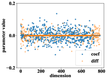
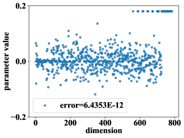
Figure 3: Left: blue dots represent computed linear regression solution $\mathbf{w}^{*}=(w^{*}_{1},\dots,w^{*}_{784})$, while orange dots show $\mathbf{w}^{*}-\mathbf{u}$. A constantly-zero tail can be observed at the end for blue dots. Right: all parameter values with absolute values $<10^{-8}$ are changed to $0.18$, the error magnitude stays the same.

When the linear system is undetermined, the linear regression software is designed to find the least $L_{2}$-norm solution to ensure uniqueness, which corresponds to introducing regularizer to the original linear regression problem. This regularization causes the free parameters to always be $0$, which forms the constantly-zero tail in Figure 3. Furthermore, we artificially modify the parameter values in the obtained solution: we change all the parameter values with an absolute value $<10^{-8}$ to a fixed value of $0.18$ as shown in Figure 3. These parameter values should correspond to dimensions that do not contribute to the final evaluation of $\tilde{g}_{784}$. Therefore, arbitrarily perturbing them should not have a substantial impact. Interestingly and as expected, the error in the resulting point-wise evaluation remains the identical as in the previous case, providing evidence that these dimensions are indeed redundant.

Theorem 2.5 suggests that the ill-posed nature of the linear regression problem may be the consequence of the submanifold, where the digit-$2$ MNIST images reside, is confined in some lower dimensional linear subspace. Analyzing the singular value of the $\mathbf{0}$-centered dataset in Figure 4, we note a $534$D linear subspace can effectively capture the dataset. This implies the digit-$2$ MNIST submanifold, embedded in $\mathbb{R}^{784}$, exhibits nonlinearity up to around $534$ dimensions, while it is flat with respect to the remaining dimensions.

To validate this observation, let $\{\mathbf{q}_{1},\mathbf{q}_{2},\dots,\mathbf{q}_{784}\}$ denote the principal components of the dataset, and we project the digit-$2$ data onto $\mathbb{R}^{534}$ using $\{\mathbf{q}_{1},\dots,\mathbf{q}_{534}\}$, and repeat a $534$-dimensional linear regression experiment similar to the one on $\mathbb{R}^{784}$. In Figure 4, we observe that the linear regression recovers the parameters with no constantly-zero tail, indicating that the regression solution is unique.

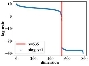
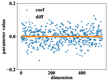
Figure 4: Left: singular value plots of the digit-$2$ images in $\mathbf{0}$-centered MNIST under log scale. A sharp decay is observed at around $\mathbf{q}_{535}$. Right: linear regression solution on the space spanned by $\{\mathbf{q}_{1},\dots\mathbf{q}_{534}\}$.

We now examine the impact of nonlinearity in the data distribution using data functions of the form: $g(\mathbf{x})=0.02\sum^{784}_{i=1}x_{i}^{2}+0.01\sum^{784}_{i=1}x_{i}$. Let $\tilde{\mathbf{x}}=(\tilde{x}_{1},\dots,\tilde{x}_{784})\in\mathbb{R}^{784}$ denote the projected data on $span\{\mathbf{q}_{1},\dots,\mathbf{q}_{534}\}$, we introduce random quadratic polynomials along all the normal directions $\{\mathbf{q}_{535},\dots,\mathbf{q}_{784}\}$ to bend the data, i.e.:

$$\bar{\mathbf{x}}(\alpha)=\tilde{\mathbf{x}}+\alpha\sum^{784}_{i=535}(\sum_{j=1}^{784}\eta_{ij}\tilde{x}_{j}^{2})\mathbf{q}_{i},$$

where $\eta_{ij}\sim\mathcal{N}(0,1)$ and $\alpha$ is the parameter to control the degree of bending. Next, we perform linear regression on $\bar{\mathbf{x}}(\alpha)$ with varying $\alpha$ to approximate the quadratic function $g$. We record the magnitude of the resulting solutions $\mathbf{w}$ as well as the magnitude of the approximation error $e_{1}=\lVert\mathbf{w}\cdot\bar{\mathbf{x}}(\alpha)-g(\bar{\mathbf{x}})\rVert$ in Table 1. We observe that as the degree of bending decreases, the pointwise approximation error on the in-sample data remains unchanged, while the magnitude of the resulting solutions increases significantly, echoing the phenomenon observed in Section 2.2.

Furthermore, we create out-of-sample data points by extending along the combined normal direction: $\mathbf{x}_{out}=\tilde{\mathbf{x}}+0.1\sum_{i=535}^{784}\mathbf{q}_{i}$, we found the “off-sample” evaluation error $e_{2}=\lVert\mathbf{w}\cdot\mathbf{x}_{out}-g(\mathbf{x}_{out})\rVert$ also drastically increases as the curvature decreases (column $4$), indicating the small amount of bending of the data manifold adversely affects the generalization to out-of-sample data.

Table 1: Magnitude of different tests of approximating a quadratic function using linear regression on full-dimensional curved data. The bending magnitude affects the linear regression solution magnitudes (column $2$) and the generalization errors (column $2$).

$\alpha$	$\lVert w\rVert_{2}$	$e_{1}$	$e_{2}$
1e-8	$92.27$	$463.21$	$2580.06$
1e-10	$7678.69$	$463.21$	$10073.15$
1e-12	$767852.03$	$463.21$	$1269868.67$

3 Regularization from noise

In Section 2, we show that local linear regression for data distributed on submanifolds can have two potential issues: (1) the problem may no have a unique solution when the data manifold is flat in one of the normal directions; (2) the nonlinearity of the data manifold could have a nontrivial effect on the first order information of the target function $g$. In this section, we investigate how the presence of noise can potentially alter these scenarios.

3.1 Noisy data could prevent degeneracy

He et al. (2023) pointed out that the presence of noise in the ambient space around the data manifold can regularize the linear regression problem. We recount their finding specifically for the simple problem considered in Section 2.1. In their setting, the data is distributed just on the $x$-axis (effectively by setting the curvature $\kappa=0$, so along the $y$-axis the data manifold is flat). Under the presence of Gaussian noise in the $y$ component of the data coordinates, i.e., $y=\sigma\eta\sim\mathcal{N}(0,\sigma^{2})$ instead of $y\equiv 0$, the optimal parameter $w_{y}^{*}$ would converge with high probability to:

$$w_{y}^{*}\sim\frac{\partial g}{\partial y}+\mathcal{O}(\frac{1}{\sigma\sqrt{N}}).$$

This implies that in the presence of noise, the previously degenerated linear system defined by the noise-free data is now invertible, and the true first-order information $\frac{\partial g}{\partial y}$ is obtained in the limit of the number of data points $N\to\infty$. This observation can be easily extended to any codimension-$k$ submanifold that is flat in certain directions to address the ill-posed linear regression as discussed in Section 2.3. A more involved example in $\mathbb{R}^{4}$ is used to demonstrate such point below:

Consider again the case of $2$-manifold embedded in $\mathbb{R}^{4}$ where the graph representation along one normal direction $y_{1}$ is at least $C^{2}$, while the graph along the other direction $y_{2}$ is only linear. Under a suitable local coordinate frame with $y_{2}\equiv 0$, the resulting system from the minimization problem is singular if one applies a full-dimensional linear regression. However, with the presence of noise, i.e., $y_{2}=\sigma\eta,~{}~{}\eta\sim\mathcal{N}(0,1)$ for some small $\sigma>0$, the linear system under our usual assumption A.1-A.4 becomes:

$$\begin{bmatrix}x_{1}&0&0&0&0\\ 0&x_{2}&0&0&0\\ 0&0&\langle y_{1}^{2}\rangle&0&\langle y_{1}\rangle\\ 0&0&0&\langle y_{2}^{2}\rangle&0\\ 0&0&\langle y_{1}\rangle&0&1\end{bmatrix}\begin{bmatrix}w_{1}\\ w_{2}\\ w_{y_{1}}\\ w_{y_{2}}\\ b\end{bmatrix}=\begin{bmatrix}\langle gx_{1}\rangle\\ \langle gx_{2}\rangle\\ \langle gy_{1}\rangle\\ \langle gy_{2}\rangle\\ \langle g\rangle\end{bmatrix}.$$

It is easy to verify that $\langle y_{2}^{2}\rangle=\sigma^{2}$, leading to $w_{y_{2}}=\frac{\partial g}{\partial y_{2}}+\mathcal{O}(\sigma^{2})$. Thus, the linear system becomes well-posed, and one can obtain the desired first-order information up to the order of noise variance.

3.2 Interplay between noises and curvatures

The second observation concerns the impact of geometry in the derived solution formulas. If one wants to use the local linear regression to obtain first-order information of the function $g$, the geometry of the data manifold would certainly affect the results as derived in Section 2.2 and Appendix B. Here we show that one simple remedy is to add noises to the data.

We demonstrate the effect of the method by applying it to the case of Section 2.1. Instead of considering $y=\kappa x^{2}$, we add the Gaussian noises to $y$ along the $y$-direction to obtain $\tilde{y}=\kappa x^{2}+\sigma\eta$. Then, the leading order solution for $w_{y}^{*}$ becomes:

$$w_{y}^{*}\sim\displaystyle\frac{\partial g}{\partial y}(0)+\frac{1}{2}\frac{\kappa L^{4}}{\kappa^{2}L^{4}+\frac{45}{4}\sigma^{2}}\frac{\partial^{2}g}{\partial x^{2}}(0),$$

instead of the previous $w_{y}^{*}\sim\frac{\partial g}{\partial y}(0)+\displaystyle\frac{1}{2\kappa}\frac{\partial^{2}g}{\partial x^{2}}(0)$. From the derived formula, we note that if we take $\sigma=0$, we recover the formula for the noise-free case. Furthermore, if we take $\sigma^{2}$ large relative to $\kappa^{2}L^{4}$, then the denominator is dominant by $\sigma^{2}$ such that $\kappa L^{4}+\frac{45}{4}\sigma^{2}\sim\frac{45}{4}\sigma^{2}$, and the overall term would be small. This suggests that by adding noises of a certain magnitude, the curvature effect would be mitigated and one can obtain a better approximation to the true first-order solution from the linear regression.

To validate the aforementioned observations, we again conduct numerical simulations under the same setting as in Section 2.1 but with added noises. We take $L=0.1$ and $\kappa=0.1$, and vary the noise standard deviation, $\sigma$, to obtain various linear regression solutions; see Figure 5.

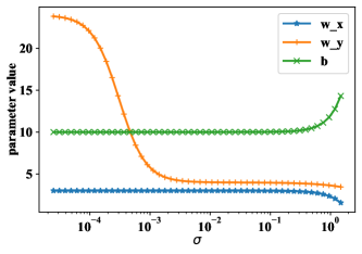
Figure 5: $2$D linear regression solutions under the presence of noises with different $\sigma$. When $\sigma$ is too small, $w_{y}^{*}$ still blows up; when $\sigma$ is of certain magnitude, $w_{y}^{*}$ approximates $\frac{\partial g}{\partial y}$; but when $\sigma$ is too large, the noise eventually affects $w_{x}^{*}$ and $b^{*}$.

Remarkably, within a suitable range of noise variance, the blow-up effect arising from a small curvature is mitigated. The underlying mechanism can be better comprehended through the visualizations of the data distribution provided in Figure 6. The intuition behind this is the addition of noise causes the data distribution to blur the structure of the problematic manifold, resulting in an improved approximation to the desired value $\frac{\partial g}{\partial y}(0)=4$.

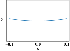
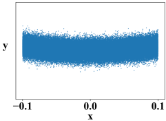
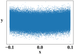
Figure 6: Visualization of the distribution of the noisy data.
(a) $\sigma=0,w_{y}^{*}=24$: the solution is influenced by the small curvature, substantially deviates from the target value $\frac{\partial g}{\partial y}=4$;
(b) $\sigma=1e-3,w_{y}^{*}=5.63$, (c) $\sigma=2e-3,w_{y}^{*}=4.43$: when noise is added at a certain level of the standard deviation $\sigma$, $w_{y}^{*}$ is significantly reduced; as $\sigma$ increases further, $w_{y}$ approaches to $4$.

4 Conclusions and future work

This study aims to investigate the impact of data manifold geometry and noise on the well-posedness and stability of local linear regression models for out-of-distribution inferences, both qualitatively and quantitatively. It was found that for general low-dimensional smooth manifolds, the uniqueness of solutions in the local linear regression problem can be compromised when the data manifold is flat in one of the normal directions. Additionally, through theoretical and experimental analysis on specific submanifolds, it was revealed that the nonlinearity of the data manifold, such as curvatures, has a significant and nontrivial effect on the stability of the regression outcomes. Furthermore, the presence of noise in the data was shown to not only prevent degeneracy but also interact with curvatures to prevent blow-up in the linear regression solutions.

This work presents a novel approach for analyzing the influence of data manifold geometry and noise on the well-posedness and stability of regression problems. It offers opportunities to incorporate established concepts and techniques from geometry to study diverse data manifolds and unveil their intrinsic impact on regression problems. Additionally, it opens avenues for exploring more complex and practical machine learning scenarios, such as investigating ReLU deep neural networks for regression and convolutional neural networks for classification tasks.

Appendix A Derivation of solutions for hypersurfaces

To compute the quantities in each entry in Equation 7, under the assumption that each $x_{i}\sim\mathcal{U}\big{(}[-L,L]\big{)}$ we have:

$$\langle x^{2}_{i}\rangle =\frac{1}{2L}\int_{-L}^{L}x^{2}_{i}\mathrm{d}x_{i}=\frac{L^{2}}{3},$$

$$\langle y\rangle =\frac{1}{(2L)^{d-1}}\int_{\Omega^{\prime}}\sum_{i=1}^{d-1}\kappa_{i}x_{i}^{2}\;\mathrm{d}x_{1}\mathrm{d}x_{2}\dots\mathrm{d}x_{d-1}=\frac{1}{(2L)}\sum_{i=1}^{d-1}\int^{L}_{-L}\kappa_{i}x_{i}^{2}\mathrm{d}x_{i}=\frac{L^{2}}{3}\sum_{i=1}^{d-1}\kappa_{i},$$

$$\langle x_{j}^{2}y\rangle =\frac{1}{(2L)}\int^{L}_{-L}\kappa_{j}x_{j}^{2}\mathrm{d}x_{j}+\frac{1}{(4L^{2})}\sum_{i=1,\,i\neq j}^{d-1}\int^{L}_{-L}\kappa_{i}x_{i}^{2}\mathrm{d}x_{i}\int^{L}_{-L}x_{j}^{2}\mathrm{d}x_{j}=\frac{L^{4}}{5}\kappa_{j}+\sum_{i=1,\,i\neq j}^{d-1}\kappa_{i}\frac{L^{4}}{9},$$

$$\langle y^{2}\rangle =\Big{\langle}(\sum_{i=1}^{d-1}\kappa_{i}x_{i}^{2})^{2}\Big{\rangle}=\Big{\langle}\sum^{d-1}_{i=1}\kappa_{i}^{2}x_{i}^{4}+2\sum_{i=2}^{d-1}\sum_{j=1}^{i}\kappa_{i}\kappa_{j}x_{i}^{2}x_{j}^{2}\Big{\rangle}=\sum_{i=1}^{d-1}\kappa_{i}^{2}\frac{L^{4}}{5}+2\sum_{i=2}^{d-1}\sum_{j=1}^{i}\kappa_{i}\kappa_{j}\frac{L^{4}}{9}.$$

The determinant of the target $2\times 2$ linear system is then given by:

$$D=\langle y^{2}\rangle-\langle y\rangle^{2}=\sum_{i=1}^{d-1}\kappa_{i}^{2}\frac{L^{4}}{5}+2\sum_{i=2}^{d-1}\sum_{j=1}^{i}\kappa_{i}\kappa_{j}\frac{L^{4}}{9}-\frac{L^{4}}{9}\big{(}\sum_{i=1}^{d-1}\kappa_{i}\big{)}^{2}$$

where $\big{(}\sum_{i=1}^{d-1}\kappa_{i}\big{)}^{2}=\big{(}\sum_{i=1}^{d-1}\kappa_{i}^{2}+2\sum_{i=2}^{d-1}\sum_{j=1}^{i}\kappa_{i}\kappa_{j}\big{)}$. As a result:

$$D=\sum_{i=1}^{d-1}\kappa_{i}^{2}(\frac{L^{4}}{5}-\frac{L^{4}}{9})=\sum_{i=1}^{d-1}\kappa_{i}^{2}\frac{4L^{4}}{45}$$

Then, to obtain an explicit expression for the RHS, we again Taylor expand the data function $g$, assumed to be locally smooth, around the base point:

$$g(\mathbf{x})=g\big{(}\mathbf{x}^{\prime},\,h(\mathbf{x}^{\prime})\big{)}=g(\mathbf{0})+\mathbf{x}^{T}\nabla g(\mathbf{0})+\frac{1}{2}\mathbf{x}^{T}Hess(g)(\mathbf{0})\mathbf{x}+O(\lVert\mathbf{x}\rVert^{3})$$

$$= g(\mathbf{0})+\frac{\partial g}{\partial y}(\mathbf{0})y+\sum_{i=1}^{d-1}\frac{\partial g}{\partial x_{i}}(\mathbf{0})x_{i}+\frac{1}{2}\sum^{d-1}_{i=1}\frac{\partial^{2}g}{\partial x_{i}^{2}}(\mathbf{0})x_{i}^{2}+\sum_{j=2}^{d-1}\sum_{i=1}^{j}\frac{\partial^{2}g}{\partial x_{i}x_{j}}(\mathbf{0})x_{i}x_{j}+\frac{1}{2}\frac{\partial^{2}g}{\partial y^{2}}(\mathbf{0})y^{2}+O(\lVert\mathbf{x}\rVert^{3})$$

where $y^{2}$ is in fact of $\mathcal{O}(\lVert x\rVert^{4})$. With such expansion along with the previously computed quantities and keeping only the nonzero terms, we can obtain $\langle g\rangle,\,\langle gx_{i}\rangle,\langle gy\rangle$ accordingly:

$$\langle g\rangle= g(\mathbf{0})+\frac{\partial g}{\partial y}(\mathbf{0})\langle y\rangle+\frac{1}{2}\sum^{d-1}_{i=1}\frac{\partial^{2}g}{\partial x_{i}^{2}}(\mathbf{0})\langle x_{i}^{2}\rangle+\Big{\langle}\mathcal{O}(\lVert\mathbf{x}\rVert^{3})\Big{\rangle}$$

$$= g(\mathbf{0})+\frac{\partial g}{\partial y}(\mathbf{0})\frac{L^{2}}{3}\sum_{i=1}^{d-1}\kappa_{i}+\frac{1}{2}\frac{L^{2}}{3}\sum^{d-1}_{i=1}\frac{\partial^{2}g}{\partial x_{i}^{2}}(\mathbf{0})+\mathcal{O}(L^{4})$$

$$\langle gx_{i}\rangle= \frac{\partial g}{\partial x_{i}}(\mathbf{0})\frac{L^{2}}{3}+\mathcal{O}(L^{4})$$

$$\langle gy\rangle= g(\mathbf{0})\langle y\rangle+\frac{\partial g}{\partial y}(\mathbf{0})\langle y^{2}\rangle+\frac{1}{2}\sum_{i=1}^{d-1}\frac{\partial^{2}g}{\partial x_{i}^{2}}\langle x_{i}^{2}y\rangle+\frac{\partial^{2}g}{\partial y^{2}}\langle y^{3}\rangle+\Big{\langle}\mathcal{O}(\lVert x\rVert^{6})\Big{\rangle}$$

$$= g(\mathbf{0})\frac{L^{2}}{3}\sum_{i=1}^{d-1}\kappa_{i}+\frac{\partial g}{\partial y}(\mathbf{0})\big{(}\sum_{i=1}^{d-1}\kappa_{i}^{2}\frac{L^{4}}{5}+2\sum_{i=2}^{d-1}\sum_{j=1}^{i}\kappa_{i}\kappa_{j}\frac{L^{4}}{9}\big{)}$$

$$+\frac{1}{2}\sum_{i=1}^{d-1}\frac{\partial^{2}g}{\partial x_{i}^{2}}(\mathbf{0})\langle\kappa_{i}x_{i}^{4}+\sum_{j\neq i}\kappa_{j}x_{i}^{2}x_{j}^{2}\rangle+\mathcal{O}(L^{6})$$

$$= g(\mathbf{0})\frac{L^{2}}{3}\sum_{i=1}^{d-1}\kappa_{i}+\frac{\partial g}{\partial y}(\mathbf{0})\big{(}\sum_{i=1}^{d-1}\kappa_{i}^{2}\frac{L^{4}}{5}+2\sum_{i=2}^{d-1}\sum_{j=1}^{i}\kappa_{i}\kappa_{j}\frac{L^{4}}{9}\big{)}$$

$$+\frac{1}{2}\sum_{i=1}^{d-1}\frac{\partial^{2}g}{\partial x_{i}^{2}}(\mathbf{0})\big{(}\kappa_{i}\frac{L^{4}}{5}+\sum_{j\neq i}\kappa_{j}\frac{L^{4}}{9}\big{)}+\mathcal{O}(L^{6})$$

Again, the optimal solutions for $w_{y},\,b$ are given by applying the inverse (the matrix is non-singular) to the RHS vector $[\langle gy\rangle,\,\langle g\rangle]^{T}$, which yields:

$$\begin{dcases}w_{y}^{*}=\frac{1}{D}\big{(}\left<gy\right>-\left<g\right>\left<y\right>\big{)}\\ b^{*}=\frac{1}{D}\big{(}\left<y^{2}\right>\left<g\right>-\left<y\right>\left<gy\right>\big{)}\end{dcases}$$

$$w_{y}^{*} =\frac{1}{\langle y^{2}\rangle-\langle y\rangle^{2}}\bigg{(}\Big{(}g(\mathbf{0})\langle y\rangle-g(\mathbf{0})\langle y\rangle\Big{)}+\Big{(}\frac{\partial g}{\partial y}(\mathbf{0})\langle y^{2}\rangle-\frac{\partial g}{\partial y}(\mathbf{0})\langle y\rangle^{2}\Big{)}$$

$$\quad+\Big{(}\frac{1}{2}\sum_{i=1}^{d-1}\frac{\partial^{2}g}{\partial x_{i}^{2}}(\mathbf{0})\big{(}\kappa_{i}\frac{L^{4}}{5}+\sum_{j\neq i}\kappa_{j}\frac{L^{4}}{9}\big{)}-\frac{1}{2}\frac{L^{2}}{3}\sum^{d-1}_{i=1}\frac{\partial^{2}g}{\partial x_{i}^{2}}(\mathbf{0})\frac{L^{2}}{3}\sum_{i=1}^{d-1}\kappa_{i}\Big{)}+\mathcal{O}(L^{6})\bigg{)}$$

$$=\frac{\partial g}{\partial y}(\mathbf{0})+\frac{1}{2D}\bigg{(}(\frac{L^{4}}{5}-\frac{L^{4}}{9})\sum_{i=1}^{d-1}\frac{\partial^{2}g}{\partial x_{i}^{2}}(\mathbf{0})\kappa_{i}+\big{(}\sum_{i=1}^{d-1}\frac{\partial^{2}g}{\partial x_{i}^{2}}(\mathbf{0})\sum_{j\neq i}\kappa_{j}-\sum_{i=1}^{d-1}\frac{\partial^{2}g}{\partial x_{i}^{2}}(\mathbf{0})\sum_{j\neq i}\kappa_{j}\big{)}\frac{L^{4}}{9}+\mathcal{O}(L^{6})\bigg{)}$$

$$=\frac{\partial g}{\partial y}(\mathbf{0})+\frac{1}{2D}\bigg{(}\frac{4L^{4}}{45}\sum_{i=1}^{d-1}\frac{\partial^{2}g}{\partial x_{i}^{2}}(\mathbf{0})\kappa_{i}+\mathcal{O}(L^{6})\bigg{)}$$

$$=\frac{\partial g}{\partial y}(\mathbf{0})+\frac{1}{2\sum_{i=1}^{d-1}\kappa_{i}^{2}\frac{4L^{4}}{45}}\bigg{(}\frac{4L^{4}}{45}\sum_{i=1}^{d-1}\frac{\partial^{2}g}{\partial x_{i}^{2}}(\mathbf{0})\kappa_{i}+\mathcal{O}(L^{6})\bigg{)}$$

$$=\frac{\partial g}{\partial y}(\mathbf{0})+\frac{1}{2}\frac{\displaystyle\sum_{i=1}^{d-1}\kappa_{i}\frac{\partial^{2}g}{\partial x_{i}^{2}}(\mathbf{0})}{\displaystyle\sum_{i=1}^{d-1}\kappa_{i}^{2}}+\mathcal{O}(L^{2})$$

$$b^{*} =\frac{1}{\langle y^{2}\rangle-\langle y\rangle^{2}}\bigg{(}g(\mathbf{0})\Big{(}\langle y^{2}\rangle-\langle y\rangle^{2}\Big{)}+\Big{(}\langle y^{2}\rangle\frac{\partial g}{\partial y}(\mathbf{0})\langle y\rangle-\langle y\rangle\frac{\partial g}{\partial y}(\mathbf{0})\langle y^{2}\rangle\Big{)}$$

$$\quad+\Big{(}\frac{1}{2}\langle y^{2}\rangle\sum_{i=1}^{d-1}\frac{\partial^{2}g}{\partial x_{i}^{2}}(\mathbf{0})\langle x_{i}^{2}\rangle-\frac{1}{2}\langle y\rangle\sum^{d-1}_{i=1}\frac{\partial^{2}g}{\partial x_{i}^{2}}(\mathbf{0})\langle x_{i}^{2}y\rangle\Big{)}+\mathcal{O}(L^{8})\bigg{)}$$

$$=g(\mathbf{0})+\frac{1}{D}\bigg{(}\Big{(}\frac{1}{2}\sum_{i=1}^{d-1}\frac{\partial^{2}g}{\partial x_{i}^{2}}(\mathbf{0})\frac{L^{2}}{3}\Big{)}\big{(}\sum_{i=1}^{d-1}\kappa_{i}^{2}\frac{L^{4}}{5}+2\sum_{i=2}^{d-1}\sum_{j=1}^{i}\kappa_{i}\kappa_{j}\frac{L^{4}}{9}\big{)}$$

$$\quad-\frac{1}{2}\frac{L^{2}}{3}\sum_{k=1}^{d-1}\kappa_{k}\sum^{d-1}_{i=1}\frac{\partial^{2}g}{\partial x_{i}^{2}}(\mathbf{0})\big{(}\kappa_{i}\frac{L^{4}}{5}+\sum_{j\neq i}\kappa_{j}\frac{L^{4}}{9}\big{)}+\mathcal{O}(L^{8})\bigg{)}$$

$$=g(\mathbf{0})+\frac{1}{D}\bigg{(}\frac{1}{2}\sum_{i=1}^{d-1}\big{(}\sum_{j=1}^{d-1}\kappa_{j}^{2}\frac{L^{6}}{15}+2\sum_{j=2}^{d-1}\sum_{k=1}^{j}\kappa_{j}\kappa_{k}\frac{L^{6}}{27}\big{)}\frac{\partial^{2}g}{\partial x_{i}^{2}}(\mathbf{0})$$

$$\quad-\frac{1}{2}\sum^{d-1}_{i=1}\Big{(}\big{(}\kappa_{i}^{2}\frac{L^{6}}{15}+\kappa_{i}\sum_{k\neq i}\kappa_{k}\frac{L^{6}}{15}\big{)}+\big{(}\kappa_{i}\sum_{j\neq i}\kappa_{j}\frac{L^{6}}{27}+(\sum_{j\neq i}\kappa_{j})^{2}\frac{L^{6}}{27}\big{)}\Big{)}\frac{\partial^{2}g}{\partial x_{i}^{2}}(\mathbf{0})+\mathcal{O}(L^{8})\bigg{)}$$

$$=g(\mathbf{0})+\frac{1}{D}\bigg{(}\frac{1}{2}\sum_{i=1}^{d-1}\big{(}\sum_{j=1}^{d-1}\kappa_{j}^{2}\frac{L^{6}}{15}+2\sum_{j=2}^{d-1}\sum_{k=1}^{j}\kappa_{j}\kappa_{k}\frac{L^{6}}{27}\big{)}\frac{\partial^{2}g}{\partial x_{i}^{2}}(\mathbf{0})$$

$$\quad-\frac{1}{2}\sum^{d-1}_{i=1}\Big{(}\big{(}\kappa_{i}^{2}\frac{L^{6}}{15}+\kappa_{i}\sum_{k\neq i}\kappa_{k}\frac{L^{6}}{15}\big{)}+\big{(}\kappa_{i}\sum_{j\neq i}\kappa_{j}+\sum_{j\neq i}\kappa_{j}^{2}+2\sum_{\begin{subarray}{c}j=2\\ j\neq i\end{subarray}}^{d-1}\sum_{\begin{subarray}{c}k=1\\ k\neq i\end{subarray}}^{j}\kappa_{j}\kappa_{k}\big{)}\frac{L^{6}}{27}\Big{)}\frac{\partial^{2}g}{\partial x_{i}^{2}}(\mathbf{0})+\mathcal{O}(L^{8})\bigg{)}$$

$$=g(\mathbf{0})+\frac{1}{2D}\sum_{i=1}^{d-1}\bigg{(}\sum_{j\neq i}\kappa_{j}^{2}(\frac{L^{6}}{15}-\frac{L^{6}}{27})-(\frac{L^{6}}{15}+\frac{L^{6}}{27})\kappa_{i}\sum_{j\neq i}\kappa_{j}+2\kappa_{i}\sum_{j\neq i}\kappa_{j}\frac{L^{6}}{27}\bigg{)}\frac{\partial^{2}g}{\partial x_{i}^{2}}(\mathbf{0})+\mathcal{O}(L^{4})$$

$$=g(\mathbf{0})+\frac{1}{2D}\sum_{i=1}^{d-1}\bigg{(}\sum_{j\neq i}\kappa_{j}^{2}(\frac{L^{6}}{15}-\frac{L^{6}}{27})-(\frac{L^{6}}{15}-\frac{L^{6}}{27})\kappa_{i}\sum_{j\neq i}\kappa_{j}\bigg{)}\frac{\partial^{2}g}{\partial x_{i}^{2}}(\mathbf{0})+\mathcal{O}(L^{4})$$

$$=g(\mathbf{0})+\frac{1}{2\displaystyle\sum_{i=1}^{d-1}\kappa_{i}^{2}\frac{4L^{4}}{45}}\sum_{i=1}^{d-1}\bigg{(}\sum_{j\neq i}\kappa_{j}^{2}(\frac{4L^{6}}{135})-(\frac{4L^{6}}{135})\kappa_{i}\sum_{j\neq i}\kappa_{j}\bigg{)}\frac{\partial^{2}g}{\partial x_{i}^{2}}(\mathbf{0})+\mathcal{O}(L^{4})$$

$$=g(\mathbf{0})+\frac{1}{2}\sum_{i=1}^{d-1}\frac{\partial^{2}g}{\partial x_{i}^{2}}(\mathbf{0})\frac{L^{2}}{3}\Big{(}\frac{\displaystyle\sum_{j\neq i}\kappa_{j}^{2}-\kappa_{i}\sum_{j\neq i}\kappa_{j}}{\displaystyle\sum_{k=1}^{d-1}\kappa_{k}^{2}}\Big{)}+\mathcal{O}(L^{4})$$

Appendix B Local linear regression for curves in $\mathbb{R}^{d}$

In this section, we consider submanifold with codimension $d-1$ in some Euclidean space, that is, a smoothly embedded curve. A simple case would be a non-planar curve in $3$-space.

B.1 Results on $3$-dimensional curves

Similar as in Section 2.2, we fix a based point $\mathbf{x}_{0}$ and apply unitary transformation and translation to obtain the standard local coordinate frame, where we have the tangent space $\mathcal{T}_{\mathbf{x}_{0}}\mathcal{M}$ as our domain. However, the caveat here is that for a curve, the tangent space is always $1$-dimensional (line induced by the tangent vector), resulting in a normal space of $2$-dimensional. Since the principal curvatures are associated to a certain normal direction, when the normal space is only $1$-dimensional, there is no ambiguity, but when the codimension is larger than $1$, one needs to deal with care as we discuss in Section 2.3.

Fortunately, for curves, a useful concept called Frenet–Serret frame from differential geometry comes in handy: if the curve $r$ is parameterized by the arc length $s$, then we have:

$$\mathcal{T}(s) =\frac{\mathbf{r}^{\prime}(s)}{|\mathbf{r}^{\prime}(s)|} \mathcal{N}(s) =\frac{\mathcal{T}^{\prime}(s)}{|\mathcal{T}^{\prime}(s)|}$$

$$\mathcal{B}(s) =\mathcal{T}(s)\times\mathcal{N}(s) \kappa(s) =|\mathcal{T}^{\prime}(s)|=|\mathbf{r}^{\prime\prime}(s)|$$

where $\mathcal{T},\,\mathcal{N},\,\mathcal{B}$ denotes the tangent direction, normal direction, and binormal direction respectively, and it is easy to see they form a orthonormal basis for the embedding space. $\kappa(s)$ denotes the curvature. Then the Frenet-Serret formulas give explicit equations to describe the relationship of the three basis vectors:

$$\begin{dcases}\mathcal{T}^{\prime}(s)=\kappa(s)\mathcal{N}(s)\\ \mathcal{N}^{\prime}(s)=-\kappa(s)\mathcal{T}(s)+\tau(s)\mathcal{B}(s)\\ \mathcal{B}^{\prime}(s)=-\tau(s)\mathcal{N}(s)\end{dcases}$$ (8)

where $\tau(s)$ is the torsion (at position $\mathbf{r}(s)$) given by $\lvert\tau(s)\rvert=\lVert\mathcal{N}^{\prime}(s)-\big{(}\mathcal{N}^{\prime}(s)\cdot\mathcal{T}(s)\big{)}\mathcal{T}(s)\rVert$, which in intuition describes the tendency of the curve to deviate from being flat in a plane, just as the curvature describes the tendency to stay away from being straight as a line. Then we arrive at the following lemma.

Lemma B.1.

(Local representation of curves in $\mathbb{R}^{3}$)
For a smoothly embedded curve $\mathbf{r}(s)$ in $3$-dimensional Euclidean space, locally when viewing from the coordinates defined through $\mathcal{T},\mathcal{N}$ and $\mathcal{B}$, it can be approximated by monomials in each of the basis direction in the following way:

$$\mathbf{r}(s)=\big{(}x,\frac{\kappa}{2}x^{2}+\mathcal{O}(x^{6}),\frac{\kappa\tau}{6}x^{3}+\mathcal{O}(x^{9})\big{)}\implies\mathbf{r}(s)\approx(x,\frac{\kappa}{2}x^{2},\frac{\kappa\tau}{6}x^{3})$$

Proof.

By taking the local referring point as $\mathbf{r}(0)=\mathbf{0}$, then a local Taylor expansion of the curve around $s=0$ yields:

$$\mathbf{r}(s)=\mathbf{0}+\mathbf{r}^{\prime}(0)(s-0)+\frac{1}{2}\mathbf{r}^{\prime\prime}(0)(s-0)^{2}+\frac{1}{6}\mathbf{r}^{\prime\prime\prime}(0)(s-0)^{3}+\mathcal{O}(s^{4})$$ (9)

Using the Frenet-Serret frame Equation 8, we know

$$\mathbf{r}^{\prime}(s) =\mathcal{T}(s)$$

$$\mathbf{r}^{\prime\prime}(s) =\mathcal{T}^{\prime}(s)=\kappa(s)\mathcal{N}(s)$$

$$\mathbf{r}^{\prime\prime\prime}(s) =\big{(}\kappa(s)\mathcal{N}(s)\big{)}^{\prime}=\kappa^{\prime}(s)\mathcal{N}(s)+\kappa(s)N^{\prime}(s)$$

$$=\kappa^{\prime}(s)\mathcal{N}(s)+\kappa(s)\big{(}-\kappa(s)\mathcal{T}(s)+\tau(s)\mathcal{B}(s)\big{)}$$

$$=\kappa^{\prime}(s)\mathcal{N}(s)-\kappa^{2}(s)\mathcal{T}(s)+\kappa(s)\tau(s)\mathcal{B}(s)$$

Plug in the above into Equation 9 to obtain:

$$\mathbf{r}(s)=\mathcal{T}s+\frac{1}{2}\kappa\mathcal{N}s^{2}+\frac{1}{6}(\kappa^{\prime}(0)\mathcal{N}-\kappa^{2}\mathcal{T}+\kappa\tau\mathcal{B})s^{3}+\mathcal{O}(s^{4})$$ (10)

which is a complete characterization of the curve $\mathbf{r}(s)$ around $s=0$ up to the forth order. Furthermore, note that $\mathcal{T}$-$\mathcal{N}$-$\mathcal{B}$ forms an orthonormal basis with the origin being at $\mathbf{0}$, we can therefore express Equation 10 up to the forth order term under the new coordinate basis by collecting terms as

$$\mathbf{r}(s)\approx\Big{(}s-\frac{\kappa^{2}}{6}s^{3},\;\frac{\kappa}{2}s^{2}+\frac{\kappa^{\prime}(0)}{6}s^{3},\;\frac{\kappa\tau}{6}s^{3}\Big{)}\implies\mathbf{r}(s)\approx\Big{(}s,\;\frac{\kappa}{2}s^{2},\;\frac{\kappa\tau}{6}s^{3}\Big{)}$$

Finally, for another parametrization of $\mathbf{r}(t)$, choose a specific $t$ such that the change along the tangent direction at $t=0$ has the same scale as the original $x$-axis. This can be easily done by setting the parametrization to have constant speed along $\mathcal{T}$, and rescale the constant to match with $x$. Thus, locally we obtain $\mathbf{r}(t)\cdot\mathcal{T}=:x(t)\sim x$, having the same scale as $x$. On the other hand, for the arc length parametrization one has

$$s(t)=\int_{0}^{t}\lVert\mathbf{r}^{\prime}(z)\rVert\mathrm{d}z$$

which is another function of $t$. Therefore, both $x(t)$ and $s(t)$ admit the Taylor series expansion around $0$ as follow:

$$s(t) =s(0)+s^{\prime}(0)t+\frac{s^{\prime\prime}(0)}{2}t^{2}+\mathcal{O}(t^{3})$$

$$x(t) =x(0)+x^{\prime}(0)t+\frac{x^{\prime\prime}(0)}{2}t^{2}+\mathcal{O}(t^{3})$$

We show their Taylor series expansions match with each other in the lower order. Apparently $s(0)=x(0)=0$, then for first order: $x^{\prime}(t)=\mathbf{r}^{\prime}(t)\cdot\mathcal{T}$, $s^{\prime}(t)=\lVert\mathbf{r}^{\prime}(t)\rVert$ by fundamental theorem of calculus. But $\mathcal{T}=\displaystyle\frac{\mathbf{r}^{\prime}(0)}{\lVert\mathbf{r}^{\prime}(0)\rVert}$, we have $x^{\prime}(0)=\lVert\mathbf{r}^{\prime}(0)\rVert=s^{\prime}(0)$. As for the second order derivative, $x^{\prime\prime}(t)=\mathbf{r}^{\prime\prime}(t)\cdot\mathcal{T}\implies x^{\prime\prime}(0)=\mathbf{r}^{\prime\prime}(0)\cdot\mathcal{T}$.

$$s^{\prime\prime}(t) =(\lVert\mathbf{r}^{\prime}(t)\rVert)^{\prime}=\frac{\big{\langle}\mathbf{r}^{\prime}(t)\,,\,\mathbf{r}^{\prime\prime}(t)\big{\rangle}+\big{\langle}\mathbf{r}^{\prime\prime}(t)\,,\,\mathbf{r}^{\prime}(t)\big{\rangle}}{2\sqrt{\big{\langle}\mathbf{r}^{\prime}(t)\,,\,\mathbf{r}^{\prime}(t)\big{\rangle}}}=\frac{\langle\mathbf{r}^{\prime}(t)\,,\,\mathbf{r}^{\prime\prime}(t)\rangle}{\lVert\mathbf{r}^{\prime}(t)\rVert}=\mathcal{T}(t)\cdot\mathbf{r}^{\prime\prime}(t)$$

which implies $s^{\prime\prime}(0)=\mathcal{T}\cdot\mathbf{r}^{\prime\prime}(0)=x^{\prime\prime}(0)$. A further calculation will show that $s^{\prime\prime\prime}(0)\neq x^{\prime\prime\prime}(0)$, therefore $s(t)-x(t)=\mathcal{O}(t^{3})$. Since $x(0)=0$, from the Taylor expansion we have $x(t)=\mathcal{O}(t)$, we can then write $s(t)=x(t)+\mathcal{O}(x(t)^{3})$. Plug this in to $\mathbf{r}(s)\approx\Big{(}s,\;\frac{\kappa}{2}s^{2},\;\frac{\kappa\tau}{6}s^{3}\Big{)}$ we have the desired results. ∎

The above formulation indicates that if we choose the tangent space as the space for the independent variable $x$, as we did in Section 2.2, and investigate the local graph representation of the curve with respect to this base coordinate, we have one graph along the $\mathcal{N}$ direction, whose approximation is denoted by $y(x)=\frac{\kappa}{2}x^{2}$, and one along the $\mathcal{B}$ direction, with approximation denoted by $z(x)=\frac{\kappa\tau}{6}x^{3}$. Therefore, we can perform local linear regression under this coordinate frame, demonstrated in the following theorem:

Theorem B.2.

(Solution formulas for local linear regression on curves in $\mathbb{R}^{3}$)
Assume for simplicity the given data points $(x,y,z)\in\mathcal{M}$ are uniform in $x$, $e.g.\;x\in\Omega=[-L,\,L]$ where $\mathcal{M}$ is a curve in $3$D, then the solution formulas for local linear regression on $\mathcal{M}$ under the local coordinate frame, if the problem is well-posed, are given by:

$$\begin{dcases}w_{x}^{*}=\frac{\partial g}{\partial x}(\mathbf{0})+\mathcal{O}(L^{4})\\ w_{y}^{*}=\frac{\partial g}{\partial y}(\mathbf{0})+\frac{1}{2k_{2}}\frac{\partial^{2}g}{\partial x^{2}}(\mathbf{0})+\mathcal{O}(L^{2})\\ w_{z}^{*}=\frac{\partial g}{\partial z}(\mathbf{0})+\frac{k_{2}}{k_{3}}\frac{\partial^{2}g}{\partial xy}(\mathbf{0})+\frac{1}{6k_{3}}\frac{\partial^{3}g}{\partial x^{3}}(\mathbf{0})+\mathcal{O}(L^{2})\\ b^{*}=g(\mathbf{0})+\mathcal{O}(L^{4})\end{dcases}$$

where $k_{2},k_{3}$ are the corresponding nonlinear quantities along the $y,z$ respectively.

Proof.

From Lemma B.1, we know any curve can be locally described by the triplet: $(x,\,\frac{\kappa}{2}x^{2},\,\frac{\kappa\tau}{6}x^{3})$ up to some higher order error, where $x$ is the independent variable along the tangent direction at the base point $\mathbf{x}_{0}=\mathbf{0}$, and $\kappa,\,\tau$ are the curvature and torsion respectively at the base point. For consistency we denote $\kappa$ by $k_{2}$ and $\tau$ by $k_{3}$, and assume they are non-zero otherwise the linear regression problem becomes ill-posed on the dimensions with zero nonlinear quantities.

Similar to Section 2.1 by a symmetry argument, $e.g.,\,\langle xy\rangle=\langle yz\rangle=0,\,\langle xz\rangle\neq 0$, the linear system resulted from the least square minimization is (with a reordering):

$$\begin{bmatrix}\langle x^{2}\rangle&\langle xz\rangle&0&0\\ \langle xz\rangle&\langle z^{2}\rangle&0&0\\ 0&0&\langle y^{2}\rangle&\langle y\rangle\\ 0&0&\langle y\rangle&1\end{bmatrix}\begin{bmatrix}w_{x}\\ w_{y}\\ w_{z}\\ b\end{bmatrix}=\begin{bmatrix}\langle gx\rangle\\ \langle gz\rangle\\ \langle gy\rangle\\ \langle g\rangle\end{bmatrix}\implies\begin{dcases}\begin{bmatrix}\langle x^{2}\rangle&\langle xz\rangle\\ \langle xz\rangle&\langle z^{2}\rangle\end{bmatrix}\begin{bmatrix}w_{x}\\ w_{z}\end{bmatrix}=\begin{bmatrix}\langle gx\rangle\\ \langle gz\rangle\end{bmatrix}\\ \\ \begin{bmatrix}\langle y^{2}\rangle&\langle y\rangle\\ \langle y\rangle&1\end{bmatrix}\begin{bmatrix}w_{y}\\ b\end{bmatrix}=\begin{bmatrix}\langle gy\rangle\\ \langle g\rangle\end{bmatrix}\end{dcases},$$

leading to two independent $2\times 2$ linear systems which can be solved exactly. ∎

Again, from the solution formula we make conclusion similar to that from Section 2.1: when any of the direction of $y$ and $z$ is flat, meaning $k_{2}=0$ or $k_{3}=0$, the linear system is not invertible hence the problem is well-posed; the non-linearity prevents the ill-posedness, but they affect the first order solution from a non-trivial way. The next step is to generalize to curves in $d$-dimensional Euclidean space.

B.2 Generalizations to curves in $\mathbb{R}^{d}$

To obtain a similar result to curves in an Euclidean space of arbitrary dimension, we first need a local representation of the curve in $\mathbb{R}^{d}$. To this end, we introduce the notion of generalized Frenet-Serret formula: starting from the canonical basis vectors, the tangent $\mathcal{T}$ and the normal $\mathcal{N}(s)=\mathcal{T}^{\prime}(s)/\lvert\mathcal{T}^{\prime}(s)\rvert$, one obtains the remaining orthonormal basis following a Gram-Schmidt type procedure by subtracting projection on previous directions. For example, to get the next two basis vectors:

$$\tau\mathcal{B}(s)=\mathcal{N}^{\prime}(s)-(\mathcal{N}^{\prime}(s)\cdot\mathcal{T}(s))\mathcal{T}(s)\implies\mathcal{N}^{\prime}(s)=-\kappa(s)\mathcal{T}(s)+\tau(s)\mathcal{B}(s)$$

$$\sigma\mathcal{D}(s)=\mathcal{B}^{\prime}(s)-(\mathcal{B}^{\prime}(s)\cdot\mathcal{N}(s))\mathcal{N}(s)-(\mathcal{B}^{\prime}(s)\cdot\mathcal{T}(s))\mathcal{T}(s)\implies\mathcal{B}^{\prime}(s)=-\tau\mathcal{N}(s)+\sigma\mathcal{D}(s),$$

where $(\tau,\,\mathcal{B})$ and $(\sigma,\,\mathcal{D})$ are the nonlinearity-direction pair for the third and the forth normal direction respectively, and the last equation follows from differentiating $\mathcal{B}\cdot\mathcal{T}=0$. Last but not least, if the curve is embedded in $\mathbb{R}^{4}$, by expressing $\mathcal{D}^{\prime}(s)$ in terms of sum of projections along all the available directions, and differentiating the dot product of $\mathcal{D}$ with all the directions, we will have $\displaystyle\mathcal{D}^{\prime}(s)=-\tau(s)\mathcal{B}(s)$. In high dimension, for clarity, we use $\{\mathcal{V}_{i}\}_{i=1}^{d}$ to denote the orthonormal basis, $e.g.\;\mathcal{V}_{1}:=\mathcal{T}$, $\mathcal{V}_{2}:=\mathcal{N}$, etc, and $\{\alpha_{i}\}_{i=1}^{d}$ for the corresponding curvature quantities, $e.g.\;\alpha_{1}=1$, $\alpha_{2}=\kappa$, etc. Then, all the corresponding Frenet equations derived from the Gram-Schmidt process can be summarized in the following matrix form (with a slight abuse of notation that $\mathcal{V}_{1}^{\prime}=\mathcal{T}^{\prime}(0)$, etc.)

$$\begin{bmatrix}0&\alpha_{2}&0&\dots&0\\ -\alpha_{2}&0&\alpha_{3}&\dots&0\\ 0&-\alpha_{3}&0&\ddots&\vdots\\ \vdots&\ddots&\ddots&\ddots&\alpha_{d}\\ 0&\dots&0&-\alpha_{d}&0\end{bmatrix}\begin{bmatrix}\mathcal{V}_{1}\\ \mathcal{V}_{2}\\ \mathcal{V}_{3}\\ \vdots\\ \mathcal{V}_{d}\end{bmatrix}=\begin{bmatrix}\mathcal{V}_{1}^{\prime}\\ \mathcal{V}_{2}^{\prime}\\ \mathcal{V}_{3}^{\prime}\\ \vdots\\ \mathcal{V}_{d}^{\prime}\end{bmatrix}$$ (11)

With Equation 11, we have the following Lemma:

Lemma B.3.

(Local representation of curves in $\mathbb{R}^{d}$)
For a smoothly embedded curve $\mathbf{r}(s)$ in $\mathbb{R}^{d}$, locally when viewing from the coordinates frame obtained by the generalized Frenet-Serret frame, it can be approximated by monomials in each of the basis direction in the following way:

$$\mathbf{r}(s)\approx(s,\,\frac{\alpha_{2}}{2}s^{2},\,\dots,\,\frac{\prod_{i=1}^{d}\alpha_{i}}{d!}s^{d})\approx(x,\,k_{2}x^{2},\dots,\,k_{d}x^{d})$$

Proof.

Note $\mathcal{V}_{1}=\mathbf{r}^{\prime}(0)$, and for $n<d$ from Equation 11, we notice:

$$\mathbf{r}^{\prime\prime}(0)=\mathcal{V}_{1}^{\prime}=\alpha_{2}\mathcal{V}_{2},\;\mathbf{r}^{\prime\prime\prime}(0)=\alpha_{2}\mathcal{V}_{2}^{\prime}=\alpha_{2}(-\alpha_{2}\mathcal{V}_{1}+\alpha_{3}\mathcal{V}_{3}),\;\mathcal{V}_{n}^{\prime}=-\alpha_{n}\mathcal{V}_{n-1}+\alpha_{n+1}\mathcal{V}_{n+1}$$

By induction, one can easily see that the $n$-th basis direction only shows up in and after the $n$-th order derivative $r^{(n)}(0)$. Combined with the Taylor series of $\mathbf{r}$ around $s=0$, by setting $\mathbf{r}(0)=0$,

$$\mathbf{r}(s)=\sum_{n=1}^{d}\frac{\mathbf{r}^{(n)}(0)}{n!}s^{n}+\mathcal{O}(s^{d+1})$$

we know that when collecting all the terms associated to $\mathcal{V}_{n}$, the leading order term is $s^{n}$. Therefore, the leading order approximation of $\mathbf{r}$ in terms of the basis $\{\mathcal{V}_{i}\}_{i=1}^{d}$ is:

$$\mathbf{r}(s)\approx(s,\,\frac{\alpha_{2}}{2}s^{2},\,\dots,\,\frac{\prod_{i=1}^{d}\alpha_{i}}{d!}s^{d})$$

Using $x_{n}$ to denote the variable corresponding to the $n$-th direction and let $k_{n}:=\frac{1}{n!}\prod_{i=1}^{n}\alpha_{i}$ to denote the corresponding nonlinear quantity, we get $x_{n}(s)=k_{n}s^{n}+\mathcal{O}(s^{n+1})$. Then by the approximation introduced in similar to Theorem B.2 , we finally arrive at the local approximation of the curve along the $n$-th direction for any $n\leq d$:

$$x_{n}(x)=k_{n}x^{n}+\mathcal{O}(x^{3(n+1)})\approx k_{n}x^{n}$$

∎

With Lemma B.3, one can follow the same procedure as in Theorem B.2 to derive the solution formula for local linear regression on curves in $\mathbb{R}^{d}$. However, the resulting linear system is dense and high dimensional where the direct solving is no longer tractable. Therefore, we consider an approach based on method of matched asymptotic (Lagerstrom, 2013) to obtain the solution formulas.

Theorem B.4.

(Solution formulas for local linear regression on curves in $\mathbb{R}^{d}$) Assume for simplicity the given data points $\mathbf{x}\in\mathcal{M}$ are uniform in $x_{1}$, $e.g.\;x_{1}\in\Omega=[-L,\,L]$ where $\mathcal{M}$ is a curve in $\mathbb{R}^{d}$, then the solution formulas for local linear regression on $\mathcal{M}$ under the local coordinate frame, if the problem is well-posed, are given by:

$$\begin{dcases}w_{n}=\sum\limits_{\{j_{i}\}\in A_{n}}\frac{\prod\limits_{i=1}k_{j_{i}}}{|\{j_{i}\}|!k_{n}}\frac{\partial^{|\{j_{i}\}|}g}{\partial x_{j_{1}}x_{j_{2}}\dots}(\mathbf{0})+\mathcal{O}\Big{(}L^{2\big{(}\left\lceil\frac{d}{2}\right\rceil-\left\lfloor\frac{n}{2}\right\rfloor\big{)}}\Big{)}\\ \,\\ b=g(\mathbf{0})+\mathcal{O}\Big{(}L^{2\big{(}\left\lceil\frac{d}{2}\right\rceil\big{)}}\Big{)}\end{dcases}.$$

where $k_{j}$ is the corresponding nonlinear quantities along the $j$-th basis direction, and $A_{n}$ is the set of all finite indexing sequences $\left\{j_{i}\right\}_{i=1}$ such that:

$$A_{n}=\left\{\,\{j_{i}\}_{i=1}\,\bigg{|}\,j_{i}\in N^{*},\,\sum_{i}j_{i}=n\right\}$$

Proof.

From Lemma B.3, variables associated to each basis direction can be expressed in terms of $x_{1}$, then by the symmetry argument:

$$\langle x_{i}x_{j}\rangle\sim\langle x_{1}^{i+j}\rangle=\begin{dcases}\langle x_{1}^{i+j}\rangle=\frac{k_{i}k_{j}}{i+j+1}L^{i+j};\;&\text{if }i+j\text{ even}\\ 0;\;&\text{if }i+j\text{ odd}\end{dcases},$$

resulting in a decoupling of the linear system from the least square minimization of linear regression problem. For example, the odd system is given as

$$\begin{bmatrix}\langle x_{1}^{2}\rangle&\langle x_{1}x_{3}\rangle&\langle x_{1}x_{5}\rangle&\dots\\ \langle x_{1}x_{3}\rangle&\langle x_{3}^{2}\rangle&\langle x_{3}x_{5}\rangle&\dots\\ \langle x_{1}x_{5}\rangle&\langle x_{3}x_{5}\rangle&\langle x_{5}^{2}\rangle&\dots\\ \vdots&\vdots&\vdots&\ddots\\ \end{bmatrix}\begin{bmatrix}w_{1}\\ w_{3}\\ w_{5}\\ \vdots\end{bmatrix}=\begin{bmatrix}\langle gx_{1}\rangle\\ \langle gx_{3}\rangle\\ \langle gx_{5}\rangle\\ \vdots\end{bmatrix},$$ (12)

Solving the above system is not tractable in high dimension, however, there is a helpful one can make use of. For example, for the first row:

$$\langle x_{1}^{2}\rangle=\frac{L^{2}}{3};\quad\langle x_{1}x_{3}\rangle=\frac{k_{3}L^{4}}{5};\quad\langle x_{1}x_{5}\rangle=\frac{k_{5}L^{6}}{7}\quad\dots$$

while for the R.H.S. $\;\langle gx_{1}\rangle$, assume $g$ has enough regularity, we Taylor expand $g$ around $\mathbf{0}$ abbreviating the evaluation at $\mathbf{0}$ notation for clarify $s.t.,\,\frac{\partial g}{\partial x_{1}}:=\frac{\partial g}{\partial x_{1}}(\mathbf{0})$:

$$\frac{\partial g}{\partial x_{1}}\langle x_{1}^{2}\rangle+\frac{\partial g}{\partial x_{3}}\langle x_{1}x_{3}\rangle+\frac{\partial^{2}g}{\partial x_{1}x_{2}}\langle x_{1}^{2}x_{2}\rangle+\frac{\partial^{2}g}{\partial x_{2}x_{3}}\langle x_{1}x_{2}x_{3}\rangle+\frac{1}{6}\frac{\partial^{3}g}{\partial x_{1}^{3}}\langle x_{1}^{4}\rangle+\frac{1}{2}\frac{\partial^{3}g}{\partial x_{1}^{2}x_{3}}\langle x_{1}^{3}x_{3}\rangle+\dots$$

$$=\frac{\partial g}{\partial x_{1}}\frac{L^{2}}{3}+\frac{\partial g}{\partial x_{3}}\frac{k_{3}L^{4}}{5}+\frac{\partial^{2}g}{\partial x_{1}x_{2}}\mathcal{O}(L^{4})+\frac{\partial^{2}g}{\partial x_{2}x_{3}}\mathcal{O}(L^{6})+\frac{1}{6}\frac{\partial^{3}g}{\partial x_{1}^{3}}L^{4}+\frac{1}{2}\frac{\partial^{3}g}{\partial x_{1}^{2}x_{3}}\mathcal{O}(L^{6})+\dots$$

Since $L\ll 1$ is a free variable, by using the idea from the method of matched asymptotic expansions, we match different orders of $L$ in the equation to obtain the solutions for $w_{i}^{*}$. In this case, for the first three variable coefficeitns, we have

$$\begin{dcases}\frac{w_{1}^{*}}{3}L^{2}=\frac{\partial g}{\partial x_{1}}\frac{L^{2}}{3}+\mathcal{O}(L^{4})\implies w_{1}^{*}=\frac{\partial g}{\partial x_{1}}+\mathcal{O}(L^{2})\\ w_{3}^{*}=\frac{\partial g}{\partial x_{3}}+\frac{k_{2}}{k_{3}}\frac{\partial^{2}g}{\partial x_{1}x_{2}}+\frac{1}{6k_{3}}\frac{\partial^{3}g}{\partial x_{1}^{3}}+\mathcal{O}(L^{2})\\ w_{5}^{*}=\frac{\partial g}{\partial x_{5}}+\frac{k_{2}k_{3}}{k_{5}}\frac{\partial^{2}g}{\partial x_{2}x_{3}}+\frac{k_{4}}{k_{5}}\frac{\partial^{2}g}{\partial x_{1}x_{4}}+\frac{k_{2}^{2}}{2k_{5}}\frac{\partial^{3}g}{\partial x_{1}x_{2}^{2}}+\frac{k_{3}}{2k_{5}}\frac{\partial^{3}g}{\partial x_{1}^{2}x_{3}}+\frac{k_{2}}{6k_{5}}\frac{\partial^{4}g}{\partial x_{1}^{3}x_{2}}+\frac{1}{120k_{5}}\frac{\partial^{5}g}{\partial x_{1}^{5}}+\mathcal{O}(L^{2})\end{dcases}$$

Last but not least, for $w_{1}^{*}$, the higher order $\mathcal{O}(L^{2})$ comes from the $\mathcal{O}(L^{4})$ terms from the R.H.S., but the existence of $w_{3}^{*}$ ensures the complete matching of the $\mathcal{O}(L^{4})$ terms, therefore, $w_{1}^{*}$ would have $\mathcal{O}(L^{4})$ as the higher order terms instead, but existence of $w_{5}^{*}$ would further turn it into $\mathcal{O}(L^{6})$. In the end, if the curve is embedded in $\mathbb{R}^{d}$ for $d$ being odd, the higher order term for $w_{1}^{*}$ would be $\mathcal{O}(L^{d-1})$, and $\mathcal{O}(L^{d})$ if $d$ is even. Similar arguments can be applied to each of the coefficients. Finally, for the even order system for $b,\,w_{2}^{*},\,w_{4}^{*},\dots$, same conclusion can be made. And by identifying the patterns in the solution formulas, one could use the following compact formula to represent:

$$\begin{dcases}w_{n}=\sum\limits_{\{j_{i}\}\in A_{n}}\frac{\prod\limits_{i=1}k_{j_{i}}}{|\{j_{i}\}|!k_{n}}\frac{\partial^{|\{j_{i}\}|}g}{\partial x_{j_{1}}x_{j_{2}}\dots}(\mathbf{0})+\mathcal{O}\Big{(}L^{2\big{(}\left\lceil\frac{d}{2}\right\rceil-\left\lfloor\frac{n}{2}\right\rfloor\big{)}}\Big{)}\\ \,\\ b=g(\mathbf{0})+\mathcal{O}\Big{(}L^{2\big{(}\left\lceil\frac{d}{2}\right\rceil\big{)}}\Big{)}\end{dcases}.$$

where $k_{j}$ is the corresponding nonlinear quantities along the $j$-th basis direction, and $A_{n}$ is the set of all finite indexing sequences $\left\{j_{i}\right\}_{i=1}$ such that:

$$A_{n}=\left\{\,\{j_{i}\}_{i=1}\,\bigg{|}\,j_{i}\in N^{*},\,\sum_{i}j_{i}=n\right\}.$$

For example, when $n=3$, $A_{n}=\left\{\,\{1,1,1\},\,\{1,2\},\{2,1\},\{3\}\,\right\}$, which are the corresponding $x$-indices for each of the term in the leading order solution for $w_{3}^{*}$. ∎

The above solution formulas indicate that when embedding the curve in an extremely high dimensional Euclidean space, the higher order term correspond to the power of $L$ would be infinitesimally small for most of the variable coefficients, while the leading order terms always remain, and we again observe the nonlinear quantities come into play in a totally non-trivial way.

References

- Abdi & Williams (2010) Abdi, H. and Williams, L. J. Principal component analysis. Wiley Interdisciplinary Reviews: Computational Statistics, 2(4):433–459, 2010.
- Ansuini et al. (2019) Ansuini, A., Laio, A., Macke, J. H., and Zoccolan, D. Intrinsic dimension of data representations in deep neural networks. Advances in Neural Information Processing Systems, 32, 2019.
- Arora et al. (2016) Arora, R., Basu, A., Mianjy, P., and Mukherjee, A. Understanding deep neural networks with rectified linear units. arXiv preprint arXiv:1611.01491, 2016.
- Babuvska & Rheinboldt (1978) Babuvska, I. and Rheinboldt, W. C. Error estimates for adaptive finite element computations. SIAM Journal on Numerical Analysis, 15(4):736–754, 1978.
- Balakrishnama & Ganapathiraju (1998) Balakrishnama, S. and Ganapathiraju, A. Linear discriminant analysis-a brief tutorial. Institute for Signal and Information Processing, 18(1998):1–8, 1998.
- Belkin & Niyogi (2003) Belkin, M. and Niyogi, P. Laplacian eigenmaps for dimensionality reduction and data representation. Neural Computation, 15(6):1373–1396, 2003.
- Bourgain et al. (2011) Bourgain, J., Dilworth, S., Ford, K., Konyagin, S., and Kutzarova, D. Explicit constructions of rip matrices and related problems. Duke Mathematical Journal, 159(1):145–185, 2011.
- Brand (2002) Brand, M. Charting a manifold. Advances in Neural Information Processing Systems, 15, 2002.
- Chen et al. (2019) Chen, M., Jiang, H., Liao, W., and Zhao, T. Efficient approximation of deep relu networks for functions on low dimensional manifolds. Advances in Neural Information Processing Systems, 32, 2019.
- Chui & Mhaskar (2018) Chui, C. K. and Mhaskar, H. N. Deep nets for local manifold learning. Frontiers in Applied Mathematics and Statistics, 4:12, 2018.
- Cleveland (1979) Cleveland, W. S. Robust locally weighted regression and smoothing scatterplots. Journal of the American Statistical Association, 74(368):829–836, 1979.
- Cleveland & Devlin (1988) Cleveland, W. S. and Devlin, S. J. Locally weighted regression: an approach to regression analysis by local fitting. Journal of the American Statistical Association, 83(403):596–610, 1988.
- Cloninger & Klock (2021) Cloninger, A. and Klock, T. A deep network construction that adapts to intrinsic dimensionality beyond the domain. Neural Networks, 141:404–419, 2021.
- Cox & Cox (2008) Cox, M. A. A. and Cox, T. F. Multidimensional scaling. In Handbook of Data Visualization, pp. 315–347. Springer, 2008.
- Dong et al. (2020) Dong, B., Ju, H., Lu, Y., and Shi, Z. Cure: Curvature regularization for missing data recovery. SIAM Journal on Imaging Sciences, 13(4):2169–2188, 2020.
- Donoho & Grimes (2003) Donoho, D. L. and Grimes, C. Hessian eigenmaps: Locally linear embedding techniques for high-dimensional data. Proceedings of the National Academy of Sciences, 100(10):5591–5596, 2003.
- Federer (1959) Federer, H. Curvature measures. Transactions of the American Mathematical Society, 93(3):418–491, 1959.
- Fefferman et al. (2016) Fefferman, C., Mitter, S., and Narayanan, H. Testing the manifold hypothesis. Journal of the American Mathematical Society, 29(4):983–1049, 2016.
- Gong et al. (2019) Gong, S., Boddeti, V. N., and Jain, A. K. On the intrinsic dimensionality of image representations. In Proceedings of the IEEE/CVF Conference on Computer Vision and Pattern Recognition, pp. 3987–3996, 2019.
- Gross et al. (2020) Gross, B. J., Trask, N., Kuberry, P., and Atzberger, P. J. Meshfree methods on manifolds for hydrodynamic flows on curved surfaces: A generalized moving least-squares (gmls) approach. Journal of Computational Physics, 409:109340, 2020.
- Hardoon et al. (2004) Hardoon, D. R., Szedmak, S., and Shawe-Taylor, J. Canonical correlation analysis: An overview with application to learning methods. Neural Computation, 16(12):2639–2664, 2004.
- He et al. (2020) He, J., Li, L., Xu, J., and Zheng, C. Relu deep neural networks and linear finite elements. Journal of Computational Mathematics, 38(3):502–527, 2020.
- He et al. (2023) He, J., Tsai, R., and Ward, R. Side effects of learning from low-dimensional data embedded in a euclidean space. Research in the Mathematical Sciences, 10(1):13, 2023.
- Hein & Maier (2006) Hein, M. and Maier, M. Manifold denoising. Advances in Neural Information Processing Systems, 19, 2006.
- Johnson & Lindenstrauss (1984) Johnson, W. B. and Lindenstrauss, J. Extensions of lipschitz mappings into a hilbert space 26. Contemporary Mathematics, 26, 1984.
- Krahmer & Ward (2011) Krahmer, F. and Ward, R. New and improved johnson–lindenstrauss embeddings via the restricted isometry property. SIAM Journal on Mathematical Analysis, 43(3):1269–1281, 2011.
- Lagerstrom (2013) Lagerstrom, P. A. Matched asymptotic expansions: ideas and techniques, volume 76. Springer Science & Business Media, 2013.
- LeCun et al. (1998) LeCun, Y., Bottou, L., Bengio, Y., and Haffner, P. Gradient-based learning applied to document recognition. Proceedings of the IEEE, 86(11):2278–2324, 1998.
- Levin (1998) Levin, D. The approximation power of moving least-squares. Mathematics of Computation, 67(224):1517–1531, 1998.
- Liang & Zhao (2013) Liang, J. and Zhao, H. Solving partial differential equations on point clouds. SIAM Journal on Scientific Computing, 35(3):A1461–A1486, 2013.
- Liu et al. (2021) Liu, H., Chen, M., Zhao, T., and Liao, W. Besov function approximation and binary classification on low-dimensional manifolds using convolutional residual networks. In International Conference on Machine Learning, pp. 6770–6780. PMLR, 2021.
- Narayanan & Mitter (2010) Narayanan, H. and Mitter, S. Sample complexity of testing the manifold hypothesis. In Proceedings of the 23rd International Conference on Neural Information Processing Systems-Volume 2, pp. 1786–1794, 2010.
- Niyogi et al. (2008) Niyogi, P., Smale, S., and Weinberger, S. Finding the homology of submanifolds with high confidence from random samples. Discrete & Computational Geometry, 39(1):419–441, 2008.
- Pedregosa et al. (2011) Pedregosa, F., Varoquaux, G., Gramfort, A., Michel, V., Thirion, B., Grisel, O., Blondel, M., Prettenhofer, P., Weiss, R., Dubourg, V., et al. Scikit-learn: Machine learning in python. the Journal of machine Learning research, 12:2825–2830, 2011.
- Pope et al. (2021) Pope, P., Zhu, C., Abdelkader, A., Goldblum, M., and Goldstein, T. The intrinsic dimension of images and its impact on learning. arXiv preprint arXiv:2104.08894, 2021.
- Roweis & Saul (2000) Roweis, S. T. and Saul, L. K. Nonlinear dimensionality reduction by locally linear embedding. Science, 290(5500):2323–2326, 2000.
- Ruderman (1994) Ruderman, D. L. The statistics of natural images. Network: Computation in Neural Systems, 5(4):517, 1994.
- Saul & Roweis (2003) Saul, L. K. and Roweis, S. T. Think globally, fit locally: Unsupervised learning of low dimensional manifolds. Journal of Machine Learning Research, 4:119–155, 2003.
- Schaefer et al. (2006) Schaefer, S., McPhail, T., and Warren, J. Image deformation using moving least squares. In ACM SIGGRAPH 2006 Papers, pp. 533–540. 2006.
- Schmidt-Hieber (2019) Schmidt-Hieber, J. Deep relu network approximation of functions on a manifold. arXiv preprint arXiv:1908.00695, 2019.
- Schölkopf et al. (1998) Schölkopf, B., Smola, A., and Müller, K.-R. Nonlinear component analysis as a kernel eigenvalue problem. Neural Computation, 10(5):1299–1319, 1998.
- Shaham et al. (2018) Shaham, U., Cloninger, A., and Coifman, R. R. Provable approximation properties for deep neural networks. Applied and Computational Harmonic Analysis, 44(3):537–557, 2018.
- Singer & Thorpe (2015) Singer, I. M. and Thorpe, J. A. Lecture notes on elementary topology and geometry. Springer, 2015.
- Tenenbaum et al. (2000) Tenenbaum, J. B., De Silva, V., and Langford, J. C. A global geometric framework for nonlinear dimensionality reduction. Science, 290(5500):2319–2323, 2000.
- Trask et al. (2019) Trask, N., Patel, R. G., Gross, B. J., and Atzberger, P. J. Gmls-nets: A framework for learning from unstructured data. arXiv preprint arXiv:1909.05371, 2019.
- Wang et al. (2010) Wang, H.-Y., Xiang, D.-H., and Zhou, D.-X. Moving least-square method in learning theory. Journal of Approximation Theory, 162(3):599–614, 2010.
- Weinberger et al. (2004) Weinberger, K. Q., Sha, F., and Saul, L. K. Learning a kernel matrix for nonlinear dimensionality reduction. In Proceedings of the 21st International Conference on Machine Learning, pp. 106, 2004.
- Zhu et al. (2018) Zhu, W., Qiu, Q., Huang, J., Calderbank, R., Sapiro, G., and Daubechies, I. Ldmnet: Low dimensional manifold regularized neural networks. In Proceedings of the IEEE Conference on Computer Vision and Pattern Recognition, pp. 2743–2751, 2018.