Efficient Information Reconciliation for High-Dimensional Quantum Key Distribution

Abstract

The Information Reconciliation phase in quantum key distribution has significant impact on the range and throughput of any QKD system. We explore this stage for high-dimensional QKD implementations and introduce two novel methods for reconciliation. The methods are based on nonbinary LDPC codes and the Cascade algorithm, and achieve efficiencies close the the Slepian-Wolf bound on q-ary symmetric channels.

1 Introduction

Quantum Key Distribution (QKD) protocols allows for secure transmission of information between two entities, Alice and Bob, by distributing a symmetric secret key via a quantum channel [1, 2]. The process involves a quantum stage where quantum information is distributed and measured. This quantum stage is succeeded by post-processing. In this purely classical stage, the results of the measurements undergo a reconciliation process to rectify any discrepancies before a secret key is extracted during the privacy amplification phase. The emphasis of this research paper is on the phase of information reconciliation, which has a significant impact on the range and throughput of any QKD system.

Despite the considerate development of QKD technology using binary signal forms, its high-dimensional counterpart (HD-QKD)[3] has seen significantly less research effort so far. However, HD-QKD offers several benefits, including higher information efficiency and increased noise resilience [4, 5, 6, 7]. Although the reconciliation phase for binary-based QKD has been extensively researched, little work has been done to analyze and optimize this stage for HD-QKD, apart from introducing the layered scheme in 2013 [8]. This study addresses this research void by introducing two novel methods for information reconciliation for high-dimensional QKD and analyzing their performance.

Unlike the majority of channel coding applications, the (HD)-QKD scenario places lesser demands on latency and throughput while emphasizing significantly the minimization of information leakage. Spurred by this unique setting, the superior decoding performance of nonbinary LDPC codes [9], and their inherent compatibility with high dimensions, we investigate the conception and utilization of nonbinary LDPC codes for post-processing in HD-QKD protocols as the first method.

The second method we investigate is the Cascade protocol [10]. It is one of the earliest proposed methods for reconciling keys. While the many rounds of communication required by Cascade and concerns about resulting limitations on throughput have led to a focus on syndrome-based methods [11, 12, 13] in the past decade, recent research has shown that sophisticated software implementations can enable Cascade to achieve high throughput even with realistic latency on the classical channel [14, 15]. Motivated by these findings, we explore the usage of Cascade in the reconciliation stage of HD-QKD and propose a modification that enables high reconciliation efficiency for the respective quantum channel.

2 Background

In this section, we describe the general setting and channel model and introduce relevant figures of merit. We then continue to describe the two proposed methods in more detail.

2.1 Information reconciliation

The goal of the information reconciliation stage in QKD is to correct any discrepancies between the keys of the two parties while minimizing the information leaked to potential eavesdroppers. Generally, Alice sends a random string $\mathbf{x}=(x_{0},...,x_{n-1})$, $x_{i}={0,...,q-1}$ of $n$ qudits of dimension $q$ to Bob, who measures them and obtains his version of the string $\mathbf{y}=(y_{0},...,y_{n-1})$, $y_{i}={0,...,q-1}$. We assume that the quantum channel can be accurately represented by a substitute channel where $\mathbf{x}$ and $\mathbf{y}$ are correlated as a $q$-ary symmetric channel since errors are typically uncorrelated and symmetric. The transition probabilities of such a channel are as follows:

$$\text{P}(y_{i}|x_{i})=\begin{cases}1-p&y_{i}=x_{i},\\ \frac{p}{q-1}&\text{else}.\end{cases}$$ (1)

Here, the parameter $p$ represents the channel transition probability. We refer to the symbol error rate between $\mathbf{x}$ and $\mathbf{y}$ as the quantum bit error rate (QBER) in a slight abuse of notation but consistent with experimental works on HD-QKD. In our simulations, we assume the QBER to be an inherent channel property, making it equivalent to the channel parameter $p$. In addition to the qudits, Alice also sends messages, e.g. syndromes or parity bits, which are assumed to be error-free. From a coding perspective, this is equal to asymmetric Slepian-Wolf coding with side information at the receiver, where the syndrome $\mathbf{s}$ represents the compressed version of $\mathbf{x}$, and $\mathbf{y}$ is the side information. A more detailed explanation of this equivalence can be found in [16], while for an interpretation of Cascade in the context of linear block codes see [17]. Any information leaked to a potential eavesdropper at any point during the quantum key distribution must be subtracted from the final secret key during privacy amplification [18]. The information leaked during the information reconciliation stage will be denoted by leak${}_{\text{IR}}$. In the case of LDPC codes, assuming no rate adaptation, it can be upper-bounded by the syndrome length in bits, $\text{leak}_{\text{IR}}\leq m$, with $m$ being the syndrome length times $\log_{2}(q)$. In the case of Cascade, it can be upper-bounded by the number of parity bits sent from Alice to Bob [19]. Using the Slepian-Wolf bound [20], the minimum amount of leaked information required to successfully reconcile with an arbitrarily low failure probability in the asymptotic limit of infinite length is given by the conditional entropy:

$$\text{leak}_{\text{IR}}\geq n\text{H}(X|Y).$$ (2)

The conditional entropy (base $q$) of the $q$-ary symmetric channel, assuming independent and identically distributed input $X$, can be expressed as

$$\text{H}(X|Y)=-((1-p)\text{log}_{q}(1-p)-p\cdot\text{log}_{q}(\frac{p}{q-1})).$$ (3)

A code’s performance in terms of relative information leakage can be measured by its efficiency $f$, given by

$$f=\frac{\text{leak}_{\text{IR}}}{n\text{H}(X|Y)}.$$ (4)

It is important to note that an efficiency of $f>1$ corresponds to leaking more bits than required by the theoretical minimum of $f=1$, which represents the best possible performance according to the Slepian-Wolf bound. In practice, systems have $f>1$ due to the difficulty of designing optimal codes, finite-size effects, and the inherit trade-off between efficiency and throughput. In the following sections, we restrict ourselves to $q$ being a power of 2. Both approaches can function without this restriction, but it allows for more efficient implementation of the reconciliation and is commonly seen in physical implementations of the quantum stage due to symmetries.

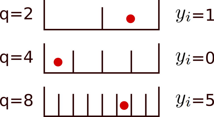
Figure 1: Example of a qudit using a time-bin implementation [21]. The dimension of the qudit is set by the number of bins grouped together, while the value is determined by the measured arrival time.

2.2 Nonbinary LDPC codes

2.2.1 Codes & Decoding

We provide here a short overview over nonbinary LDPC codes and their decoding based on the concepts and formalism of binary LDPC codes. For a comprehensive review of those, we refer to [22].
Nonbinary LDPC codes can be described by their parity check matrix $\mathbf{H}$, with $m$ rows and $n$ columns, containing elements in a Galois Field (GF) of order $q$. To enhance clarity in this section, all variables representing a Galois field element will be marked with a hat, for instance, $\hat{a}$. Moreover, let $\oplus,\ominus,\otimes,$ and $\oslash$ denote the standard operations on Galois field elements. An LDPC code can be depicted as a bipartite graph, known as the Tanner graph. In this graph, the parity-check equations form one side, called check nodes, while the codeword symbols represent the other side, known as variable nodes. The Tanner graph of a nonbinary LDPC code also has weighted edges between check and variable nodes, where the weight corresponds to the respective entry of $\mathbf{H}$. The syndrome $\mathbf{s}$ of the $q$-ary string $\mathbf{x}$ is computed as $\mathbf{s}=\mathbf{H}\mathbf{x}$.

For decoding, we employ a log-domain FFT-SPA [23, 24]. In-depth explanations of this algorithm can be found in [25, 26], but we provide a summary here for the sake of completeness. Let $Z$ represent a random variable taking values in GF($q$), such that $\text{P}(Z_{i}=k)$ indicates the probability that qudit $i$ has the value $k=0,...,q-1$. The probability vector $\mathbf{p}=(p_{0},...p_{q-1})$, $p_{j}=\text{P}(Z=j)$, can be converted into the log-domain using the generalized equivalent of the log-likelihood-ratio (LLR) in the binary case, $\mathbf{m}=(m_{0},...,m_{q-1})$, $m_{j}=\text{log}\frac{\text{P}(Z=0)}{\text{P}(Z=j)}=\log(\frac{p_{0}}{p_{j}})$. Given the LLR representation, probabilities can be retrieved through $p_{j}=\exp(-m_{j})/\sum_{k=0}^{q-1}\exp(-m_{k})$. We use $p(\cdot)$ and $m(\cdot)$ to denote these transforms. To further streamline notation, we define the multiplication and division of an element $\hat{a}$ in GF$(q)$ and an LLR message as a permutation of the indices of the vector:

$$\hat{a}\cdot\mathbf{m} :=(m_{\hat{0}\oslash\hat{a}},...,m_{\hat{q-1}\oslash\hat{a}})$$ (5)

$$\mathbf{m}/\hat{a} :=(m_{\hat{0}\otimes\hat{a}},...,m_{\hat{q-1}\otimes\hat{a}}),$$ (6)

where the multiplication and division of the indices occur in the Galois Field. These permutations are necessary as we need to weigh messages according to their edge weight during decoding. We further define two transformations involved in the decoding,

$$\bar{\mathcal{F}}(\mathbf{m},\hat{H}{ij}) =\mathcal{F}(p(\hat{H}{ij}\cdot\mathbf{m}))$$ (7)

$$\bar{\mathcal{F}}(\mathbf{m},\hat{H}{ij})^{-1} =m(\mathcal{F}^{-1}(\mathbf{m}))/\hat{H}{ij},$$ (8)

where $\mathcal{F}$ represents the discrete Fourier transform. Note that for $q$ being a power of 2, the Fast Walsh Hadamard Transform can be utilized. The decoding process then consists of two iterative message-passing phases, from check nodes to variable nodes and vice versa. The message update rule at iteration $l$ for the check node corresponding to the parity check matrix entry at $(i,j)$ can be expressed as

$$\mathbf{m}^{(l)}_{ij,\text{CV}}=\mathcal{A}(\hat{s}^{\prime}_{i})\bar{\mathcal{F}}^{-1}(\underset{j\prime\in\mathcal{M}(i)/j}{\Pi}\bar{\mathcal{F}}(\mathbf{m}^{(l-1)}_{ij\prime},\hat{H}_{ij\prime}),\hat{H}_{ij}),$$ (9)

where $\mathcal{M}(i)$ denotes the set of all check nodes in row $i$ of $\mathbf{H}$. $\mathcal{A}$, defined as $\mathcal{A}_{kj}(\hat{a})=\delta(\hat{a}\oplus k\ominus j)-\delta(a\ominus j)$, accounts for the nonzero syndrome [26]. The weighted syndrome value is calculated as $\hat{s}^{\prime}_{i}=\hat{s}_{i}\oslash\hat{H}_{ij}$. The a posteriori message of column $j$ can be written as

$$\tilde{\mathbf{m}}^{(l)}_{j}=\mathbf{m}^{(0)}(j)+\underset{i^{\prime}\in\mathcal{N}(j)}{\sum}\mathbf{m}^{(l)}_{i^{\prime}j,\text{CV}},$$ (10)

where $\mathcal{N}(j)$ is the set of all check nodes in column $j$ of $\mathbf{H}$. The best guess $\tilde{\mathbf{x}}$ at each iteration $l$ can be calculated as the minimum value of the a posteriori, $\tilde{x}_{j}^{(l)}=\text{argmin}(\tilde{\mathbf{m}}^{l}_{j})$. The second message passings, from variable to check nodes, are given by

$$\mathbf{m}_{ij,\text{VC}}^{(l)}=\tilde{\mathbf{m}}^{(l)}_{j}-\mathbf{m}^{(l)}_{ij,\text{CV}}.$$ (11)

The message passing continues until either $\mathbf{H}\tilde{\mathbf{x}}=\mathbf{s}$ or the maximum number of iterations is reached.

To allow for efficient reconciliation for different QBER values, a rate-adaptive scheme is required. We use the blind reconciliation protocol [27]. A fixed fraction $\delta$ of symbols is chosen to be punctured or shortened. Puncturing refers to replacing a key bit with a random bit that is unknown to Bob, for shortening the value of the bit is additionally send to Bob over the public channel. Puncturing, therefore, increases the code rate, while shortening lowers it. The rate of a code with $p$ punctured and $s$ shortened bits is then given by

$$R=\frac{n-m-s}{n-p-s}.$$ (12)

To see how rate adaption influences the bounding of $\text{leak}_{\text{IR}}$ see [28]. The blind scheme introduces interactivity into the LDPC reconciliation. Given a specific code, we start out with all bits being punctured and send the respective syndrome to Bob. Bob attempts to decode using the syndrome. If decoding fails, Alice transforms $\lceil n(0.028-0.02R)\rceil$ [29] punctured bits into shortened bits, and resends the syndrome. This value is a heuristic expression and presents a trade-off between the number of communication rounds and the efficiency. Bob tries to decode again and requests more bits to be shortened in case of failure. If there are no punctured bits left to be turned into shortened bits, Alice reveals key bits instead. This continues until either decoding succeeds or the the whole key is revealed.

2.2.2 Density Evolution

In the case of a uniform edge weight distribution, the asymptotic decoding performance of LDPC codes for infinite code length is entirely determined by two polynomials [30, 31]:

$$\lambda(x)=\sum_{i=0}^{d_{\text{v, max}}}\lambda_{i}x^{i-1}\quad\rho(x)=\sum_{i=0}^{d_{\text{c, max}}}\rho_{i}x^{i-1}.$$ (13)

In these expressions, $\lambda_{i}$ ($\rho_{i}$) represents the proportion of edges connected to variable (check) nodes with degree $i$, while $d_{\text{v, max}}$ ($d_{\text{c, max}}$) indicates the highest degree of the variable (check) nodes. Given these polynomials, we can then define the code ensemble $\mathcal{E}(\lambda,\rho)$, which represents all codes of infinite length with degree distributions specified by $\lambda$ and $\rho$. The threshold $p_{t}(\lambda,\rho)$ of the code ensemble $\mathcal{E}(\lambda,\rho)$ is defined as the worst channel parameter (QBER) at which decoding remains possible with an arbitrarily small failure probability. This threshold can be estimated using Monte-Carlo Density Evolution (MC-DE), which is thoroughly described in [32]. This technique repeatedly samples node degrees according to $\lambda$ and $\rho$, and draws random connections between nodes for each iteration. With a sufficiently large sample size, this simulates the performance of a cycle-free code. Note that MC-DE is particularly well suited for nonbinary LDPC codes, as the distinct edge weights aid in decorrelating messages [32]. During the simulation, we track the average entropy of all messages. When it falls below a certain value, decoding is considered successful. If this does not occur after a maximum number of iterations, the evaluated channel parameter is above the threshold of $\mathcal{E}(\lambda,\rho)$. Utilizing a concentrated check node distribution (which is favorable according to [33]) and a fixed code rate, we can further simplify to $\mathcal{E}(\lambda)$. The threshold can then be employed as an objective function to optimize the code design, which is commonly achieved using the Differential Evolution algorithm [34].

2.3 Cascade

2.3.1 Binary Cascade

Cascade [10] is one of the earliest schemes proposed for information reconciliation and has seen widespread use due to its simplicity and high efficiency. Cascade operates in several iterative steps. Alice and Bob divide their strings into top-level blocks of size $k_{1}$ and calculate their parity, where the size $k_{1}$ usually depends on the QBER and the specific version of Cascade. They send and compare their parities over a noiseless classical channel. If the parities for a single top-level block do not match, they perform a binary search on this block. There, the block is further divided into two, and parities are calculated and compared again. One of the two sub-blocks will have a different parity than the corresponding sub-block of Alice. We continue the binary search on this sub-block until we reach a sub-block that has size one, which allows us to locate and correct one error per mismatched top-level block. Alice and Bob then move on to the next iteration, where they shuffle their strings and choose new top-level blocks of size $k_{2}$. They then repeat the binary search on those. After correcting a bit in iteration $i$, except for $i=1$, Bob can look for blocks in previous iterations that contain this specific bit. The parity of these blocks has now changed as the bit got flipped, mismatching now with Alice’s parity. This allows Bob to perform another binary search on them and correct additional bits. He can then again look for these additional bits in all earlier iterations, allowing for detected errors to ”cascade” back. Successive works on the original Cascade protocol have been trying to increase its performance by either substituting the parity exchange with error-correction methods [35], or by optimizing parameters like the top-level block sizes [36]. All our comparisons and modifications are applied to a high performing modifications [17] achieving efficiencies of up to $f=1.025$. This version has also been the basis for a recent high-throughput implementation, reaching a throughput of up to $570$ Mbps [14].

2.3.2 High-Dimensional Cascade

We propose the following modification to use Cascade for high-dimensional data, which we will denote by high-dimensional Cascade (HD-Cascade). We only highlight the differences compared to the best-performing approach[17] in terms of efficiency designed for binary QKD.

1. Initially, we map all symbols to an appropriate binary representation. Prior to the first iteration, we shuffle all bits while maintaining a record of which bits originate from the same symbol. This mapping effectively reduces the expected QBER used for block-size calculations to $\text{QBER}_{\text{BIN}}=q/(2(q-1))\text{QBER}_{\text{SYM}}$.
   

2. Upon detecting an error, we immediately request the values of all bits originating from the same symbol, if not already known. The conditional probability to be a one given the values of all previously transmitted bits for these bits is close to $1/2$. To be precise, it is equal to $1/2$ for bits that have not yet participated in any parity checks and then varies with the length of the smallest block they participated in [17]. If any of these bits are erroneous, the blocks they have been participating in now have a mismatching parity. We can therefore immediately run the cascading step on those requested bits in all iterations including the current one, detecting more errors. Note that this allows for a cascading process in the first iteration already.
   

3. The fraction of errors corrected in the first iteration is significantly higher (often $>95\%$ in our simulations) compared to the binary version. This is due to the possibility of running a cascading process in the first iteration already. Consequently, we need to increase the block sizes for the following iterations as the dimensionality increases, see Table 2.

3 Results

3.1 Nonbinary LDPC codes

While the code-design and decoding techniques described above are feasible for any dimension $q$, we focus on $q=4$, $8$ as those are common in current implementations [37]. Nine codes were designed with code rates between 0.50 and 0.90 for $q=4$ ($q=8)$, corresponding to a QBER range between $0$ and $18\%$ ($24.7\%$). We used 100000 nodes with a maximum of 150 iterations for the MC-DE, the QBER was swept in 20 steps in a short range below the best possible threshold. In the Differential Evolution, population sizes between 15 and 50, a differential weight of 0.85, and a crossover probability of 0.7 were used. A sparsity of at most 10 nonzero coefficients in the polynomial was enforced, with the maximum node degree chosen as $d_{\text{v, max}}=40$. The sparsity allowed for reasonable optimization complexity, the maximum node degree was chosen to avoid numerical instability which we observed for higher values.

The results of the optimization can be found in Table 1 in form of the node degree distributions and their performance according to density evolution. The efficiency was evaluated for the highest sustainable QBER. The all-zero codeword assumption was used for the optimization and evaluation, which holds for the given scenario of a symmetric channel [25]. For all rates, the designed thresholds are close to the theoretical bound. LDPC codes with a length of $n=30000$ symbols were constructed using Progressive Edge Growth [38], and a log-FFT-SPA decoder was used to reconcile the messages. The simulated performance of the finite-size codes can be seen in Figure 5 for a span of different QBER values, each data point being the mean of 100 samples. We used the blind reconciliation scheme for rate-adaption. The mean number of decoding tries required for Bob to successfully reconcile is also shown. The valley pattern visible in the efficiency of the LDPC codes is due to the switching between codes of different rate, and a slight degradation in performance for high ratios of puncturing or shortening. The decoder used a maximum of 100 decoding iterations. As expected for finite-size codes, they do not reach the asymptotic ensemble threshold but show sub-optimal performance [26].

Table 1: Degree distributions for 4- and 8-dimensional nonbinary LDPC codes. The threshold calculated by Density Evolution (DET), the corresponding ensemble efficiency (EEff) and the node degree distribution in edge view.

	4-Dimensional
Rate	DET	EEff	Ensemble (edge view)
0.90	0.022	1.067	$\lambda(x)=0.069x+0.207x^{2}+0.051x^{5}+0.235x^{6}+0.070x^{14}+0.225x^{17}$
			$+0.139x^{28}$
0.85	0.037	1.045	$\lambda(x)=0.094x+0.210x^{2}+0.217x^{6}+0.088x^{9}+0.040x^{10}+0.118x^{22}$
			$+0.159x^{24}+0.071x^{28}$
0.80	0.053	1.044	$\lambda(x)=0.102x+0.204x^{2}+0.116x^{5}+0.088x^{7}+0.174x^{14}+0.107x^{26}$
			$+0.205x^{27}$
0.75	0.069	1.053	$\lambda(x)=0.107x+0.245x^{3}+0.192x^{6}+0.034x^{9}+0.207x^{18}+0.161x^{25}$
			$+0.049x^{27}$
0.70	0.08	1.054	$\lambda(x)=0.113x+0.245x^{2}+0.143x^{4}+0.081x^{10}+0.066^{14}+0.147^{16}$
			$+0.034x^{23}+0.168x^{24}$
0.65	0.11	1.045	$\lambda(x)=0.133x+0.213x^{2}+0.207x^{5}+0.014x^{8}+0.022x^{17}+0.171x^{19}$
			$+0.237x^{27}$
0.60	0.13	1.047	$\lambda(x)=0.172x+0.252x^{2}+0.216x^{6}+0.022x^{11}++0.075x^{12}+0.077x^{18}$
			$+0.183x^{20}$
0.55	0.15	1.041	$\lambda(x)=0.177x+0.279x^{2}+0.147x^{7}+0.035x^{8}++0.088x^{10}+0.129x^{14}$
			$+0.143x^{25}$
0.50	0.18	1.037	$\lambda(x)=0.184x+0.245x^{2}+0.087x^{6}+0.156x^{7}++0.067x^{17}+0.020^{21}$
			$+0.196^{25}+0.041^{28}$
	8-Dimensional
0.90	0.031	1.060	$\lambda(x)=0.112x+0.103x^{2}+0.194x^{3}+0.146x^{9}+0.163x^{10}+0.003x^{17}$
			$+0.173x^{19}+0.049x^{26}+0.006x^{28}+0.052x^{29}$
0.85	0.052	1.080	$\lambda(x)=0.125x+0.165x^{2}+0.163x^{5}+0.11x^{7}+0.073x^{12}+0.089x^{18}$
			$+0.122x^{27}+0.154x^{32}$
0.80	0.072	1.038	$\lambda(x)=0.146x+0.177x^{2}+0.130x^{4}+0.084x^{7}+0.149x^{10}+0.035x^{19}$
			$+0.029x^{22}+0.087x^{25}+0.163x^{26}$
0.75	0.096	1.030	$\lambda(x)=0.165x+0.192x^{2}+0.092x^{5}+0.176x^{7}+0.019x^{10}+0.086x^{17}$
			$+0.129x^{19}+0.103x^{30}+0.038x^{31}$
0.70	0.121	1.032	$\lambda(x)=0.160x+0.208x^{2}+0.140x^{5}+0.096x^{8}+0.028x^{10}+0.013x^{11}$
			$+0.113x^{18}+0.032x^{21}+0.211x^{27}$
0.65	0.147	1.032	$\lambda(x)=0.173x+0.228x^{2}+0.092x^{4}+0.169x^{8}+0.112x^{14}+0.019x^{23}$
			$+0.012x^{24}+0.195x^{28}$
0.60	0.177	1.026	$\lambda(x)=0.192x+0.196x^{2}+0.222x^{5}+0.104x^{13}+0.114x^{23}+0.055x^{25}$
			$+0.117x^{27}$
0.55	0.207	1.024	$\lambda(x)=0.183x+0.269x^{2}+0.124x^{6}+0.036x^{8}+0.097x^{10}+0.004^{21}$
			$+0.116x^{25}+0.171x^{26}$
0.50	0.239	1.024	$\lambda(x)=0.215x+0.256x^{2}+0.030x^{4}+0.154x^{7}+0.065x^{11}+0.050^{13}$
			$+0.072x^{21}+0.128x^{27}$

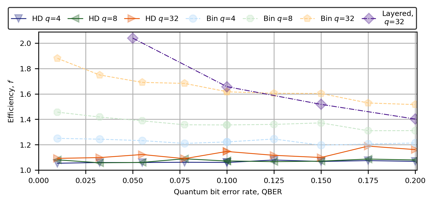
Figure 2: Efficiency of different approaches evaluated on a $q$-ary symmetric channel. Layered refers to the layered scheme, Bin to direct application of binary Cascade, and HD to the high-dimensional Cascade proposed in this work. Data points represent the mean of 1000 samples and have a FER of less than $1\%$.

3.2 High-dimensional Cascade

The performance of HD-Cascade was evaluated on the q-ary symmetric channel for dimensions $q=4$, $8$, $32$, and for a QBER ranging from $1\%$ to $20\%$. The results are shown in Figure 2. For comparison, a direct application of the best-performing Cascade modification on a binary mapping is also included. The proposed high-dimensional Cascade uses the same base Cascade with the additional adaptations discussed earlier. For $q=2$, HD-Cascade reduces to binary Cascade, resulting in equal performance. Both methods use the same block size of $n=2^{16}$ bits for all cases. The used top-level block sizes $k_{i}$ for each iteration $i$ can be seen in Table 2, where $[\cdot]$ denotes rounding to the nearest integer. Additionally, the layered scheme is included as a reference. All data points have a frame error rate below 1% and show an average of 1000 samples. The wave pattern observable for the efficiency of Cascade in Figure 2 and Figure 5 is due to the integer rounding operation when calculating the block-sizes. This seems to be unavoidable, as block-sizes being a power of two have been shown to be optimal for the binary search in this setting [17].

Table 2: Block sizes used for HD-Cascade.

$k_{1}$				$\min(2^{[\log_{2}(1/\text{QBER}_{\text{BIN}})]},n/2)$
$k_{2}$				$\min(2^{[\log_{2}(2q/\text{QBER}_{\text{BIN}})]},n/2)$
$k_{3}$	$k_{4}$	$k_{5}$	$k_{6}$	$n/16$	$n/8$	$n/4$	$n/2$

The increase in both the range and secret key rate resulting from using HD-Cascade instead of directly applying binary Cascade is depicted in Figure 3. The improvement in the relative secret key rate $r$ obtained using HD-Cascade is shown in Figure 5. This is calculated as $r=\text{skr}_{\text{HD-Cascade}}/\text{skr}_{\text{Cascade}}-1$. The used protocols are [39, 40], and experimental parameters for the simulation are derived from [41] for $q=2$, $4$, where a combination of polarization and path is used to encode the qudits. For $q=4$, we also analyzed the performance of HD-Cascade on a subset of the actual experimental data, which confirms the simulated performance. For $q=8$, $32$ we used a generalization, additional losses might transpire due to increased experimental complexity which are not considered in the simulation.

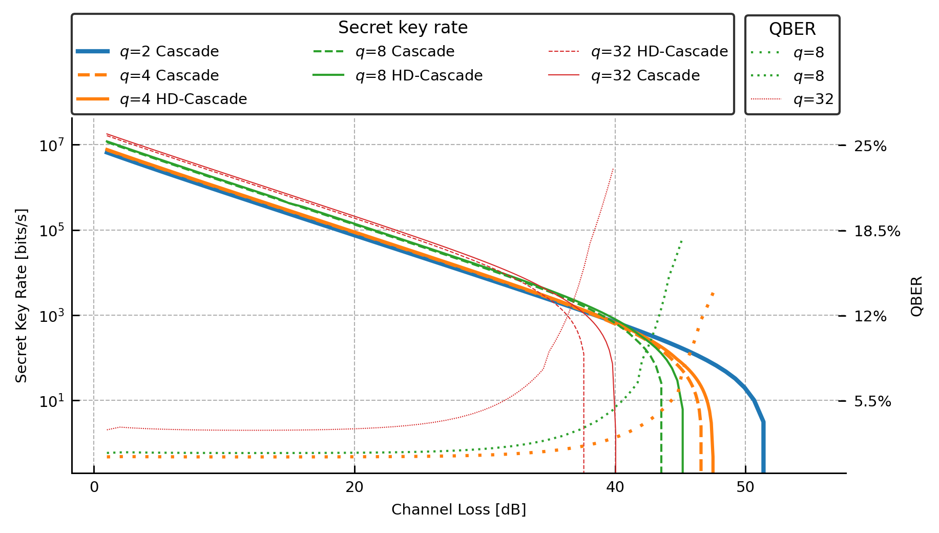
Figure 3: Secret key rate vs. channel loss for different dimensions. The decreasing dotted/dashed lines show results for direct application of binary Cascade whereas the solid lines show the performance for HD-Cascade. The increasing dotted/dashed lines show the respective QBER.

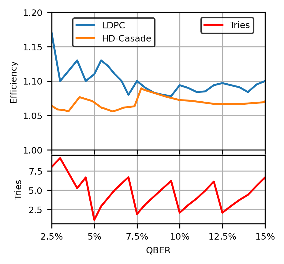
Figure 4: Top: Efficiency of using nonbinary LDPC codes and HD-Cascade for different QBER values for $q=8$. Bottom: Number of decoding tries in the blind scheme used for the LDPC codes.

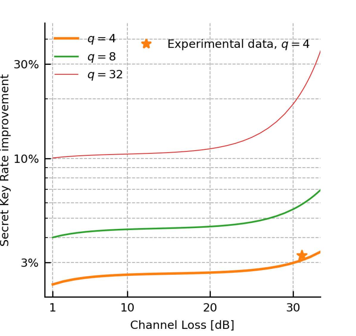
Figure 5: Relative improvement of the secret key rate for using HD-Cascade compared to binary Cascade. Experimental data provided by recent experiment[41].

4 Discussion

4.1 Nonbinary LDPC codes

Nonbinary LDPC codes are a natural candidate for the information reconciliation stage of HD-QKD, as their order can be matched to the dimension of the used qudits, and they are known to have good decoding performance [9]. Although they typically come with increased decoding complexity, this drawback is less of a concern in this context, since the keys can be processed and stored before being employed in real-time applications, which reduces the significance of decoding latency. Nevertheless, less complex decoder algorithms like EMS [42] or TEMS [43] can be considered to allow the usage of longer codes and for increasing the throughput.

The node degree distributions we constructed show ensemble efficiencies close to one, $1.037-1.067$ for $q=4$ and $1.024-1.080$ for $q=8$. Note, that to the best of our knowledge, there is no inherent reason for the efficiencies of $q=8$ to be lower than for $q=4$, it is rather just a heuristic result due to optimization parameters fitting better. Although the ensembles we found display thresholds near the Slepian-Wolf bound, we believe that even better results could be achieved by expanding the search of the hyperparameters involved in the optimization, such as the enforced sparsity and the highest degree of $\lambda$, and by performing a finer sweep of the QBER during density evolution. The evaluated efficiency of finite-size codes shows them performing significantly worse than the thresholds computed with density evolution, with efficiencies ranging from $1.078$ to $1.14$ for QBER values in a medium range. This gap can be reduced by using longer codes and improving the code construction, e.g. using improved versions of the PEG algorithm [44, 45]. The dependency of the efficiency on the QBER can further be reduced, i.e. flatting the curve in Figure 5, by improving the position of punctured bits [46].

While working on this manuscript, the usage of nonbinary LDPC codes for information reconciliation has also been proposed in [47]. They suggest mapping symbols of high dimensionality to symbols of lower dimensionality but still higher than 2 if beneficial, in similarity to the layered scheme. This can further be used to decrease computational complexity if required.

4.2 HD-Cascade

HD-Cascade has improved performance on high-dimensional QKD setups compared to directly applying binary Cascade. We can see significant improvement in efficiency, with mean efficiencies of $f_{\text{HD-Cascade}}=1.06$, $1.07$, $1.12$ compared to $f_{\text{Cascade}}=1.22$, $1.36$, $1.65$ for $q=4$, $8$, $32$, respectively. Using the parameters of a recent experimental implementation of 4-dimensional QKD[41], a resulting improvement in range and secret key rate can be observed, especially for higher dimensions. For $q=32$, an increase of more than $10\%$ in secret key rate and an additional $2.5$ dB in tolerable channel loss is achievable according to our simulation results.

Our approach demonstrates high efficiency across all QBER values but we noted that the time required for executing the correction increases significantly with higher error rates. Apart from the inherent scaling of Cascade with the QBER that is also present for binary implementations, this is additionally attributable to the immediate cascading of same-symbol bits. While the many rounds of communication required by Cascade have raised concerns about resulting limitations on throughput, recent research has shown that sophisticated software implementations can enable Cascade to achieve high throughput even with realistic latency on the classical channel [14, 15]. We expect HD-Cascade to reach similar rates as its classical counterpart, as we expect the main difference with respect to throughput being an increased difficulty to batch together parity requests for parallelization due to the additional serial cascading for the same symbol bits while keeping the resulting penalty to efficiency minimal. Moreover, we believe that significant improvements in efficiency can still be achieved by further optimizing the choice of block sizes.

4.3 Comparison

Before comparing HD-Cascade and nonbinary LDPC codes, we want to mention the layered scheme, a binary LDPC code based scheme introduced in 2013. The layered scheme is based on decoding bit layers separately using $\lceil\log_{2}(q)\rceil$ binary LDPC codes. It is similar in concept to the multilevel coding and multistage decoding methods used in slice reconciliation for continuous-variable (CV) QKD [48]. While the layered scheme allows for reconciliation using binary LDPC codes only, it brings its own drawbacks, like error propagation, bit mapping, and interactive communication. Its performance can be seen for $q=32$ in Figure 3, notably for a much smaller block length (data read off Figure 5 [8]). Later experimental implementations report efficiencies of 1.25 [49] ($q=3$, $n=1944$, $p=8\%$) and 1.17 [50] ($q=1024$, $n=4000$, $p=39.6\%)$. These papers report their efficiencies in the $\beta$-notation. $\beta$ is commonly used in the continuous-variable QKD community, whereas $f$ is more widespread with respect to discrete-variable QKD. They can be related via

$$\beta(\text{H}(X)-\text{H}(X|Y))=\text{H}(X)-f\text{H}(X|Y).$$ (14)

Overall, HD-Cascade and nonbinary LDPC codes show good efficiency over all relevant QBER values, with HD-Cascade performing slightly better in terms of efficiency (see Figure 5). HD-Cascade shows a flat efficiency behavior over all ranges, compared to the LDPC codes, which have a bad performance for very low QBER values and an increase in performance with increasing QBER. This behavior can also be observed in LDPC codes used in binary QKD [51, 52, 53]. While the focus of this work lies in introducing new methods for high-dimensional information reconciliation with good efficiencies, the throughput is another important measure, especially with continuously improving input rates from advancing QKD hardware implementation. While an absolute and direct comparison of throughput strongly depends on the specific implementation and setup parameters, relative performances can be considered. Cascade has low computational complexity but high interactivity which can limit throughput in scenarios where the classical channel has a high latency. For a constant efficiency, as approximately observed for Cascade, the number of messages exchanged scales with the QBER as it is proportional to $\text{H}(X|Y)$. Nonbinary LDPC codes, on the other hand, have low requirements on interactivity (usually below 10 syndromes per frame using the blind scheme) but high computational costs at the decoder. Their decoding complexity scales with $q$ but not with the QBER, as its main dependence is on the number of entries in its parity check matrix and the node degrees. It should be noted that the QBER is usually fairly stable until the loss approaches the maximum range of the setup, e.g. see Figure 3, and that higher dimensions tend to operate at higher QBER values. It should be emphasized that for QKD, latency is not a big issue as keys do not need to be available immediately but can be stored for usage. QKD systems are usually significantly bigger and more expensive than setups for classical communication. This allows for reconciliation schemes with comparatively high latency and high computational complexity, for example by extensive usage of pipelining [54, 14, 55].

5 Conclusion

We introduced two new methods for the information reconciliation stage of high dimensional Quantum Key Distribution. The nonbinary LDPC codes we designed specifically for the $q$-ary symmetric channel allow for reconciliation with good efficiency with low interactivity. High-dimensional Cascade on the other hand uses a highly interactive protocol with low computational complexity. It shows significant improvement compared to directly applying Cascade protocols designed for binary Quantum Key Distribution, e.g. more than $10\%$ for a 32-dimensional system for all possible channel losses.

Competing Interests

The authors declare no competing financial or non-financial interests.

Data Availability

All data used in this work are available from the corresponding author upon reasonable request.

References

- [1] C. H. Bennett and G. Brassard. Quantum cryptography: Public key distribution and coin tossing. In Proceedings of IEEE International Conference on Computers, Systems, and Signal Processing, page 175, India, 1984.
- [2] S. Pirandola, U. L. Andersen, L. Banchi, M. Berta, D. Bunandar, R. Colbeck, D. Englund, T. Gehring, C. Lupo, C. Ottaviani, J. L. Pereira, M. Razavi, J. Shamsul Shaari, M. Tomamichel, V. C. Usenko, G. Vallone, P. Villoresi, and P. Wallden. Advances in quantum cryptography. Advances in Optics and Photonics, 12(4):1012, dec 2020.
- [3] Daniele Cozzolino, Beatrice Da Lio, Davide Bacco, and Leif Katsuo Oxenlø we. High-dimensional quantum communication: Benefits, progress, and future challenges. Advanced Quantum Technologies, 2(12):1900038, 2019.
- [4] H. Bechmann-Pasquinucci and W. Tittel. Quantum cryptography using larger alphabets. Phys. Rev. A, 61:062308, May 2000.
- [5] Murphy Yuezhen Niu, Feihu Xu, Jeffrey H. Shapiro, and Fabian Furrer. Finite-key analysis for time-energy high-dimensional quantum key distribution. Phys. Rev. A, 94:052323, Nov 2016.
- [6] Sebastian Ecker, Frédéric Bouchard, Lukas Bulla, Florian Brandt, Oskar Kohout, Fabian Steinlechner, Robert Fickler, Mehul Malik, Yelena Guryanova, Rupert Ursin, and Marcus Huber. Overcoming noise in entanglement distribution. Phys. Rev. X, 9:041042, Nov 2019.
- [7] Daniele Cozzolino, Beatrice Da Lio, Davide Bacco, and Leif Katsuo Oxenløwe. High-dimensional quantum communication: Benefits, progress, and future challenges. Advanced Quantum Technologies, 2(12):1900038, oct 2019.
- [8] Hongchao Zhou, Ligong Wang, and Gregory Wornell. Layered schemes for large-alphabet secret key distribution. In 2013 Information Theory and Applications Workshop (ITA), pages 1–10, 2013.
- [9] M.C. Davey and D.J.C. MacKay. Low density parity check codes over gf(q). In 1998 Information Theory Workshop (Cat. No.98EX131), pages 70–71, 1998.
- [10] Gilles Brassard and Louis Salvail. Secret-key reconciliation by public discussion. In Tor Helleseth, editor, Advances in Cryptology — EUROCRYPT ’93, pages 410–423, Berlin, Heidelberg, 1994. Springer Berlin Heidelberg.
- [11] Jesus Martinez-Mateo, David Elkouss, and Vicente Martin. Blind reconciliation, 2013.
- [12] Evgeniy O. Kiktenko, Aleksei O. Malyshev, and Aleksey K. Fedorov. Blind information reconciliation with polar codes for quantum key distribution. IEEE Communications Letters, 25(1):79–83, jan 2021.
- [13] Jesus Martinez-Mateo, David Elkouss, and Vicente Martin. Key reconciliation for high performance quantum key distribution. Scientific Reports, 3(1):1576, Apr 2013.
- [14] Hao-Kun Mao, Qiong Li, Peng-Lei Hao, Bassem Abd-El-Atty, and Abdullah M. Iliyasu. High performance reconciliation for practical quantum key distribution systems, 2021.
- [15] Thomas Brochmann Pedersen and Mustafa Toyran. High performance information reconciliation for qkd with cascade, 2013.
- [16] A.D. Liveris, Zixiang Xiong, and C.N. Georghiades. Compression of binary sources with side information at the decoder using ldpc codes. IEEE Communications Letters, 6(10):440–442, 2002.
- [17] Christoph Pacher, Philipp Grabenweger, Jesús Martinez Mateo, and Vicente Martin. An information reconciliation protocol for secret-key agreement with small leakage. pages 730–734, 06 2015.
- [18] Kamil Brádler, Mohammad Mirhosseini, Robert Fickler, Anne Broadbent, and Robert Boyd. Finite-key security analysis for multilevel quantum key distribution. New Journal of Physics, 18(7):073030, jul 2016.
- [19] Hoi-Kwong Lo. Method for decoupling error correction from privacy amplification. New Journal of Physics, 5:36–36, apr 2003.
- [20] D. Slepian and J. Wolf. Noiseless coding of correlated information sources. IEEE Transactions on Information Theory, 19(4):471–480, 1973.
- [21] Alberto Boaron, Boris Korzh, Raphael Houlmann, Gianluca Boso, Davide Rusca, Stuart Gray, Ming-Jun Li, Daniel Nolan, Anthony Martin, and Hugo Zbinden. Simple 2.5 GHz time-bin quantum key distribution. Applied Physics Letters, 112(17):171108, apr 2018.
- [22] Shu Lin and Juane Li. Fundamentals of Classical and Modern Error-Correcting Codes. Cambridge University Press, 2022.
- [23] S. Aruna and M. Anbuselvi. Fft-spa based non-binary ldpc decoder for ieee 802.11n standard. In 2013 International Conference on Communication and Signal Processing, pages 566–569, 2013.
- [24] H. Wymeersch, H. Steendam, and M. Moeneclaey. Log-domain decoding of ldpc codes over gf(q). In 2004 IEEE International Conference on Communications (IEEE Cat. No.04CH37577), volume 2, pages 772–776 Vol.2, 2004.
- [25] Ge Li, Ivan J. Fair, and Witold A. Krzymien. Density evolution for nonbinary ldpc codes under gaussian approximation. IEEE Transactions on Information Theory, 55(3):997–1015, 2009.
- [26] Elsa Dupraz, Valentin Savin, and Michel Kieffer. Density evolution for the design of non-binary low density parity check codes for slepian-wolf coding. IEEE Transactions on Communications, 63(1):25–36, 2015.
- [27] Jesus Martinez-Mateo, David Elkouss, and Vicente Martin. Blind reconciliation. Quantum Info. Comput., 12(9–10):791–812, sep 2012.
- [28] David Elkouss, Jesús Martínez-Mateo, and Vicente Martín. Secure rate-adaptive reconciliation. In 2010 International Symposium On Information Theory and Its Applications, pages 179–184, 2010.
- [29] E. O. Kiktenko, A. S. Trushechkin, C. C. W. Lim, Y. V. Kurochkin, and A. K. Fedorov. Symmetric blind information reconciliation for quantum key distribution. Phys. Rev. Appl., 8:044017, Oct 2017.
- [30] Valentin Savin. Non binary ldpc codes over the binary erasure channel: Density evolution analysis. In 2008 First International Symposium on Applied Sciences on Biomedical and Communication Technologies, pages 1–5, 2008.
- [31] T.J. Richardson and R.L. Urbanke. The capacity of low-density parity-check codes under message-passing decoding. IEEE Transactions on Information Theory, 47(2):599–618, 2001.
- [32] Matteo Gorgoglione, Valentin Savin, and David Declercq. Optimized puncturing distributions for irregular non-binary ldpc codes. In 2010 International Symposium On Information Theory & Its Applications, pages 400 – 405, 11 2010.
- [33] Sae-Young Chung, T.J. Richardson, and R.L. Urbanke. Analysis of sum-product decoding of low-density parity-check codes using a gaussian approximation. IEEE Transactions on Information Theory, 47(2):657–670, 2001.
- [34] Rainer Storn and Kenneth Price. Differential evolution - a simple and efficient heuristic for global optimization over continuous spaces. Journal of Global Optimization, 11:341–359, 01 1997.
- [35] W. T. Buttler, S. K. Lamoreaux, J. R. Torgerson, G. H. Nickel, C. H. Donahue, and C. G. Peterson. Fast, efficient error reconciliation for quantum cryptography. Phys. Rev. A, 67:052303, May 2003.
- [36] Jesus Martinez-Mateo, Christoph Pacher, Momtchil Peev, Alex Ciurana, and Vicente Martin. Demystifying the information reconciliation protocol cascade, 2014.
- [37] Xiao-Min Hu, Chao Zhang, Yu Guo, Fang-Xiang Wang, Wen-Bo Xing, Cen-Xiao Huang, Bi-Heng Liu, Yun-Feng Huang, Chuan-Feng Li, Guang-Can Guo, Xiaoqin Gao, Matej Pivoluska, and Marcus Huber. Pathways for entanglement-based quantum communication in the face of high noise. Phys. Rev. Lett., 127:110505, Sep 2021.
- [38] Xiao-Yu Hu, E. Eleftheriou, and D.M. Arnold. Regular and irregular progressive edge-growth tanner graphs. IEEE Transactions on Information Theory, 51(1):386–398, 2005.
- [39] Davide Rusca, Alberto Boaron, Fadri Grünenfelder, Anthony Martin, and Hugo Zbinden. Finite-key analysis for the 1-decoy state QKD protocol. Applied Physics Letters, 112(17):171104, apr 2018.
- [40] Ilaria Vagniluca, Beatrice Da Lio, Davide Rusca, Daniele Cozzolino, Yunhong Ding, Hugo Zbinden, Alessandro Zavatta, Leif K. Oxenløwe, and Davide Bacco. Efficient time-bin encoding for practical high-dimensional quantum key distribution. Physical Review Applied, 14(1), jul 2020.
- [41] M. Zahidy, D. Ribezzo, C. De Lazzari, I Vagniluca, N. Biagi, T. Occhipinti, L. K. Oxenløwe, M. Galili, T. Hayashi, C. Antonelli, A. Mecozzi, A. Zavatta, and D. Bacco. 4-dimensional quantum key distribution protocol over 52-km deployed multicore fibre. In 2022 European Conference on Optical Communication (ECOC), pages 1–4, 2022.
- [42] David Declercq and Marc Fossorier. Decoding algorithms for nonbinary ldpc codes over gf. IEEE Transactions on Communications, 55(4):633–643, 2007.
- [43] Erbao Li, Kiran Gunnam, and David Declercq. Trellis based extended min-sum for decoding nonbinary ldpc codes. In 2011 8th International Symposium on Wireless Communication Systems, pages 46–50, 2011.
- [44] Hua Xiao and A.H. Banihashemi. Improved progressive-edge-growth (peg) construction of irregular ldpc codes. IEEE Communications Letters, 8(12):715–717, 2004.
- [45] Auguste Venkiah, David Declercq, and Charly Poulliat. Randomized progressive edge-growth (randpeg). In 2008 5th International Symposium on Turbo Codes and Related Topics, pages 283–287, 2008.
- [46] Matteo Gorgoglione, Valentin Savin, and David Declercq. Optimized puncturing distributions for irregular non-binary ldpc codes. In 2010 International Symposium On Information Theory and Its Applications, pages 400–405, 2010.
- [47] Debarnab Mitra, Lev Tauz, Murat Can Sarihan, Chee Wei Wong, and Lara Dolecek. Non-binary ldpc code design for energy-time entanglement quantum key distribution, 2023.
- [48] G. Van Assche, J. Cardinal, and N.J. Cerf. Reconciliation of a quantum-distributed gaussian key. IEEE Transactions on Information Theory, 50(2):394–400, 2004.
- [49] Jingyuan Liu, Zhihao Lin, Dongning Liu, Xue Feng, Fang Liu, Kaiyu Cui, Yidong Huang, and Wei Zhang. High-dimensional quantum key distribution using energy-time entanglement over 242 km partially deployed fiber, 2022.
- [50] Tian Zhong, Hongchao Zhou, Robert D. Horansky, Catherine Lee, Varun B. Verma, Adriana E. Lita, Alessandro Restelli, Joshua C. Bienfang, Richard P. Mirin, Thomas Gerrits, Sae Woo Nam, Francesco Marsili, Matthew D. Shaw, Zheshen Zhang, Ligong Wang, Dirk Englund, Gregory W. Wornell, Jeffrey H. Shapiro, and Franco N. C. Wong. Photon-efficient quantum key distribution using time-energy entanglement with high-dimensional encoding. New Journal of Physics, 17(2):022002, February 2015.
- [51] Kenta Kasai, Ryutaroh Matsumoto, and Kohichi Sakaniwa. Information reconciliation for qkd with rate-compatible non-binary ldpc codes. In 2010 International Symposium On Information Theory and Its Applications, pages 922–927, 2010.
- [52] David Elkouss, Anthony Leverrier, Romain Alleaume, and Joseph J. Boutros. Efficient reconciliation protocol for discrete-variable quantum key distribution. In 2009 IEEE International Symposium on Information Theory, pages 1879–1883, 2009.
- [53] Haokun Mao, Qiong Li, Qi Han, and Hong Guo. High-throughput and low-cost ldpc reconciliation for quantum key distribution. Quantum Information Processing, 18(7):232, Jun 2019.
- [54] Shen-Shen Yang, Jian-Qiang Liu, Zhen-Guo Lu, Zeng-Liang Bai, Xu-Yang Wang, and Yong-Min Li. An fpga-based ldpc decoder with ultra-long codes for continuous-variable quantum key distribution. IEEE Access, 9:47687–47697, 2021.
- [55] Ke Cui, Jian Wang, Hong-Fei Zhang, Chun-Li Luo, Ge Jin, and Teng-Yun Chen. A real-time design based on fpga for expeditious error reconciliation in qkd system. IEEE Transactions on Information Forensics and Security, 8(1):184–190, 2013.