Janus Collaboration

Quantifying memory in spin glasses

Abstract

Rejuvenation and memory, long considered the distinguishing features of spin glasses, have recently been proven to result from the growth of multiple length scales. This insight, enabled by simulations on the Janus II supercomputer, has opened the door to a quantitative analysis. We combine numerical simulations with comparable experiments to introduce two coefficients that quantify memory. A third coefficient has been recently presented by Freedberg et al. We show that these coefficients are physically equivalent by studying their temperature and waiting-time dependence.

Memory is among the most striking features of far-from-equilibrium systems Keim et al. (2019), including granular materials Bandi et al. (2018), phase separation in the early universe Koide et al. (2006) and, particularly, glass formers Ozon et al. (2003); Bellon et al. (2000); Yardimci and Leheny (2003); Bouchaud et al. (2001); Mueller and Shchur (2004); Scalliet and Berthier (2019); Pashine et al. (2019). Whether a universal mechanism is responsible for memory in all these materials is unknown, but spin glasses stand out Lefloch et al. (1992); Jonason et al. (1998); Lundgren et al. (1983); Jonsson et al. (1999); Hammann et al. (2000); Vincent (2007, 2023). On the one hand, memory effects are particularly strong in these systems —perhaps because of the large attainable coherence lengths Zhai et al. (2019, 2020); Paga et al. (2021). More importantly, their dynamics is now understood in great detail. Indeed, to model protocols where temperature is varied, one must first understand the nonequilibrium evolution at constant temperature. In other words, before tackling memory, rejuvenation and aging should be mastered. These intermediate steps, including the crucial role of temperature chaos, have now been taken for spin glasses Baity-Jesi et al. (2018, 2021); Zhai et al. (2022).

In the context of spin glasses, rejuvenation is the observation that when the system is aged at a temperature $T_{1}$ for a time $t_{\mathrm{w1}}$, and then cooled to a sufficiently lower $T_{2}$, the spin glass reverts apparently to the same state it would have achieved had it been cooled directly to $T_{2}$. That is, its apparent state is independent of its having approached equilibrium at temperature $T_{1}$. However, when the spin glass is then warmed back to temperature $T_{1}$, it appears to return to its aged state, hence memory.

Conventional wisdom has long ascribed rejuvenation to temperature chaos —the notion that equilibrium states at close temperatures are unrelated— and memory was experimentally exhibited long ago Lefloch et al. (1992); Jonason et al. (1998) but these effects remained unassailable to numerical simulations in three-dimensional systems Komori et al. (2000); Picco et al. (2001); Berthier and Bouchaud (2002); Takayama and Hukushima (2002); Maiorano et al. (2005); Jiménez et al. (2005). This state of affairs has recently changed Baity-Jesi et al. (2023), thanks to the combination of multiple advances: the availability of the Janus II supercomputer Baity-Jesi et al. (2014) and of single-crystal experiments Zhai et al. (2019), accessing much larger coherence lengths; the establishment of a relation between experimental and numerical time scales Zhai et al. (2020); Paga et al. (2021); and the quantitative modelling of nonequilibrium temperature chaos Baity-Jesi et al. (2021). Ref. Baity-Jesi et al. (2023) has not only demonstrated memory numerically but also shown that this effect is ruled by multiple length scales, setting the stage for a more quantitative study.

Here we introduce two coefficients to quantify memory, one experimentally accessible and the other adapted to numerical work. The example of temperature chaos has shown that such indices are key to a comprehensive theory Fernandez et al. (2013); Fernández et al. (2016); Billoire et al. (2018). In principle, the only constraints for such a coefficient $\mathcal{C}$ are that $\mathcal{C}=1$ means perfect memory and $\mathcal{C}=0$ means that the memory has been totally erased. Many choices could satisfy these conditions: besides the coefficients introduced herein, Freedberg et al. (2023) presents an alternative based on a different observable. Fortunately, the length scales discussed in Baity-Jesi et al. (2023) allow us to express these coefficients as smooth functions of similar scaling parameters and to demonstrate that they have the same physics as temperature and waiting time are varied.

Protocols.

In both experiment and simulations Paga et al. (2023), we have a three-step procedure: (i) the system is quenched to an aging temperature $T_{1}<T_{\mathrm{g}}$ ($T_{\mathrm{g}}$ is the glass temperature) and relaxes for a time $t_{\mathrm{w1}}$. In simulations, this quench is instantaneous, while in experiment, it is done at $\approx$ 10 K/min. A protocol where $T$ is kept constant after the initial quench is termed native. (ii) The system is then quenched to $T_{2}<T_{1}$, where it evolves for time $t_{\mathrm{w2}}$. (iii) The system is raised back to $T_{1}$, instantaneously in simulations, and at the same rate as cooling in experiment. After a short time at $T_{1}$ ($2^{10}$ time steps in simulations), the dynamics are compared to the native system, which has spent $t_{\mathrm{w1}}$ at $T_{1}$. The temperature drop $T_{1}-T_{2}$ is chosen to ensure that temperature chaos (and, hence, rejuvenation) is sizeable Zhai et al. (2022); Baity-Jesi et al. (2023). Our experiments are performed on a sample with $T_{\mathrm{g}}=41.6$ K. For experimental parameters see Table 1 (Table 2 for simulations).

Length scales.

Memory and rejuvenation are ruled by several related length scales (see Appendix  B for details), of which only one is experimentally accessible —$\xi_{\mathrm{Zeeman}}$, related to the Zeeman effect Joh et al. (1999). In simulations, the basic length is the size of glassy domains in a native protocol, $\xi_{\mathrm{micro}}^{\mathrm{native}}$.

We regard rejuvenation as a consequence of temperature chaos. If the temperature drop meets the chaos requirement, namely the chaos length scale set by $T_{1}-T_{2}$ is small compared to $\xi_{\mathrm{micro}}^{\mathrm{native}}(T_{1},t_{\mathrm{w1}})$ Zhai et al. (2022); Baity-Jesi et al. (2023), the system that has aged at the starting temperature $T_{1}$ for $t_{\mathrm{w1}}$ “rejuvenates” at the cold temperature $T_{2}$. That is, preexisting correlated spins are “frozen” dynamically at $T_{2}$ and a new correlated state of size $\zeta^{\mathrm{jump}}(T_{2},t_{\mathrm{w}})$ forms, where $t_{\mathrm{w}}$ is the waiting time at $T_{2}$. The newly created correlated state at $T_{2}$ is independent from that formed at $T_{1}$.

As $t_{\mathrm{w}}$ increases at $T_{2}$, the newly correlated state at $T_{2}$ grows larger, to a maximum size set by the final time at $T_{2}$, $t_{\mathrm{w2}}$. Upon heating back to $T_{1}$, the two correlated states interfere, causing a memory loss that will be seen both in experiment and simulations.

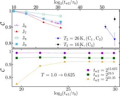
Figure 1: Memory coefficient as a function of $t_{\mathrm{w1}}$ and $t_{\mathrm{w2}}$. Top: Memory loss as a function of time $t_{\mathrm{w2}}$ both for our experiments (Table 1) and for our simulations (Table  2). The “natural” timescale $\tau_{0}$ is $1.86\times 10^{-13}$ seconds for the experimental data and $1$ lattice sweep for simulations. Bottom: Memory coefficient for fixed $t_{\mathrm{w1}}$ [fixed $\xi_{\mathrm{micro}}(T_{1},t_{\mathrm{w1}})$] and several $t_{\mathrm{w2}}$.

Protocol	$T_{1}$ (K)	$t_{\mathrm{w1}}$ (h)	$T_{2}$ (K)	$t_{\mathrm{w2}}$ (h)	$T_{\mathrm{m}}$ (K)	$\xi/a$
N1	30	1	—	—	30	13.075
N2	26	1/6	—	—	26	8.1011
N3	26	3	—	—	26	11.961
N4	16	3	—	—	16	6.3271
R1	30	1	26	3	26	11.787
C1	30	1	26	1/6	30	12.621
C2	30	1	26	3	30	12.235
C3	30	1	16	3	30	12.846

Table 1: Parameters of our experiments. We use the abbreviations N (native), R (rejuvenation) and C (cycle), see paragraph Protocols for discussion. Unlike in rejuvenation protocols, in temperature cycles the temperature is brought back to $T_{1}$ before measurements start. We indicate the measuring temperature $T_{\mathrm{m}}$, and —whenever possible— the value of $\xi$, in units of the average distance between nearest-neighbour spins. Measurements start after $t_{\mathrm{w1}}$ for native protocols ($t_{\mathrm{w1}}+t_{\mathrm{w2}}$ for cycle or rejuvenation protocols). The data for $\text{N}_{2}$ were taken at small values of $H$ because non-linear effects enter for larger values of $H$ at small $t_{\mathrm{w}}$.

Simulations can easily access $\xi_{\mathrm{micro}}^{\mathrm{native}}$ and $\zeta^{\mathrm{jump}}$ Belletti et al. (2008, 2009); Baity-Jesi et al. (2018, 2023). Experiments measure instead the number of correlated spins $N_{\text{c}}$ Joh et al. (1999). Equivalently, in simulations, the native protocol results in

$${N_{\mathrm{c}}}(T,t_{\mathrm{w}})=\bigl{[}\xi_{\mathrm{micro}}^{\mathrm{native}}(T,t_{\mathrm{w}})\bigr{]}^{D-\tfrac{\theta}{2}}\,,$$ (1)

where $\theta$ is the replicon exponent Baity-Jesi et al. (2017a); Zhai et al. (2020); Paga et al. (2021, 2022). If the chaos condition is met, and only in this case, the jump protocol results in, concomitantly,

$${N_{\mathrm{c}}}(T_{2},t_{\mathrm{w2}})\propto\bigl{[}\zeta^{\mathrm{jump}}(T_{2},t_{\mathrm{w2}})\bigr{]}^{D-\tfrac{\theta}{2}}.$$ (2)

Therefore, when chaos is strong enough, we have a dictionary relating the experimentally accessible ${N_{\mathrm{c}}}$ to these two basic length scales Baity-Jesi et al. (2023) (see Appendix B for details).

Qualitative behavior of the memory coefficient.

According to the above, one would expect memory to depend on the ratio $\zeta^{\mathrm{jump}}(T_{2},t_{\mathrm{w2}})/\xi_{\mathrm{micro}}^{\mathrm{native}}(T_{1},t_{\mathrm{w1}})$: the smaller the ratio, the larger the memory. Because both lengths are increasing functions of time, then (i) memory should increase with increasing $t_{\mathrm{w1}}$, everything else held constant. Concomitantly, (ii) memory should decrease with increasing $t_{\mathrm{w2}}$, everything else held constant. Finally, (iii) if $\Delta T=T_{1}-T_{2}$ increases, everything else held constant, $\zeta^{\mathrm{jump}}(T_{2},t_{\mathrm{w2}})$ will progressively decrease, and memory should increase. The memory coefficients that we define below, plotted in Fig. 1, display precisely these predicted variations. The experimental data in Fig. 1 agree with this expectation, which we shall test in our simulations through a scaling analysis.

Figure 2: Rejuvenation (top) and memory (bottom), as studied through the Zeeman-effect method of Ref. Joh et al. (1999) on a single crystal of CuMn. Our thermal protocols are described in Tab. 1. We show $t^{\mathrm{eff}}_{\mathrm{w}}$ vs $H^{2}$ in logarithmic scale [$t^{\mathrm{eff}}_{\mathrm{w}}(H)$ is the time at which the relaxation function (3) peaks]. The number of correlated spins $N_{\text{c}}$ for a given protocol is proportional to the slope of the corresponding curve. The values of $t^{\mathrm{eff}}_{\mathrm{w}}$ essentially coincide for native protocol N₃ and for rejuvenation protocol R₁ at $T_{2}=26$ K (the previous relaxation at $T_{1}=30$ K undergone in protocol R₁ turns out to be irrelevant at 26 K). As for the memory coefficient, see Eq. (4), the slope of native protocol N₁ is approached either by decreasing the relaxation time $t_{\mathrm{w2}}$ at fixed $T_{2}$ (compare cycles C₁ and C₂) or by lowering $T_{2}$ at fixed $t_{\mathrm{w2}}$ (compare cycles C₂ and C₃).

Experimental definition of the memory coefficient.

We define a memory coefficient from the number of correlated spins $N_{\text{c}}$, see Eq. (1). We shall first show that rejuvenation can be observed from $N_{\text{c}}$, thus confirming that temperature chaos is strong enough given our choice of temperatures and waiting times.

A small sample was cut from a single crystal of CuMn, 7.92 at.%, with $T_{\mathrm{g}}=41.6$ K. $T_{1}$ and $t_{\mathrm{w1}}$ in Table 1 were chosen to facilitate direct comparison with the results of Freedberg et al. Freedberg et al. (2023), who defined another memory coefficient from the linear magnetic susceptibility. The lower temperature, $T_{2}$, was variable, as was the waiting time $t_{\mathrm{w2}}$. Our measurements of $N_{\text{c}}$ follows Ref. Joh et al. (1999) and are illustrated in Fig. 2–top. For the reader’s convenience, we briefly recall the main steps leading to the measurement of $N_{\text{c}}$ (see Appendix D for further details).

After the sample has undergone the appropriate preparatory protocol, we probe its dynamic state by switching on a magnetic field. We set time $t=0$ when the field is switched on and record the magnetization $M(t)$, which grows steadily from $M(t=0)=0$, to obtain the dynamic response function

$$S(t,H)=\frac{1}{H}\frac{\mathrm{d}M}{\mathrm{d}\log t}\,.$$ (3)

For native protocols and $H\rightarrow 0$, the peak of $S(t)$ against $t$ occurs approximately at the effective time $t^{\mathrm{eff}}_{\mathrm{w}}\approx t_{\mathrm{w1}}$. As $H$ increases, the peak moves to shorter $t^{\mathrm{eff}}_{\mathrm{w}}(H)$. The slope of the plot of $\log t^{\mathrm{eff}}_{\mathrm{w}}~{}\mathrm{vs}~{}H^{2}$ equals the product of ${N_{\mathrm{c}}}$ times the field-cooled susceptibility per spin: ($\chi_{\text{FC}}/{\text{spin}}){N_{\mathrm{c}}}$ —$\chi_{\text{FC}}$ is roughly constant over the measured temperature range. We thus gain access to ${N_{\mathrm{c}}}$.

We compare in Fig. 2–top the outcome of the above measuring procedure as obtained in protocols N₃ and R₁ (see Table 1). The two systems evolve for the same time at 26 K. The values obtained for $\log t^{\mathrm{eff}}_{\mathrm{w}}$ turned out to be nearly identical: relaxation at 30 K does not leave measurable traces at 26 K, hence rejuvenation.

To quantify memory, we compare ${N_{\mathrm{c}}}$ for systems that have undergone the temperature-cycling protocols in Table 1 with their native counterparts. These measurements are illustrated in Fig. 2–bottom. We define the Zeeman-effect memory coefficient as

$${\cal C}_{\text{Zeeman}}={N_{\text{c}}^{\text{cycle}}}/{N_{\text{c}}^{\text{native}}}\,.$$ (4)

Note that in both cases measurements are carried out at $T_{1}$ (the difference lies in the previous thermal history of the sample), hence the ratio in Eq. (4) is just the ratio of the corresponding slopes in Fig. 2–bottom. Our results for ${\cal C}_{\text{Zeeman}}$ are given in Fig. 1.

$T$-drop	$T_{1}$	$T_{2}$	$t_{\mathrm{w1}}$	$\xi_{\mathrm{micro}}(T_{1},t_{\mathrm{w1}})$
J1	1.0	0.625	$2^{19.5}$	8.038(1)
J2	1.0	0.625	$2^{22}$	10.085(15)
J3	1.0	0.625	$2^{24.625}$	12.75(3)
J4	1.0	0.625	$2^{27.25}$	16.04(3)
J5	1.0	0.625	$2^{28.625}$	18.08(5)
J6	1.0	0.625	$2^{29.875}$	20.20(8)
J7	1.0	0.7	$2^{29.875}$	20.20(8)
J8	0.9	0.5	$2^{31.25}$	16.63(5)
J9	0.9	0.7	$2^{31.25}$	16.63(5)

Table 2: Building blocks ($T$-drop) for temperature cycles in our simulation. The initially disordered system relaxes for a time $t_{\mathrm{w1}}$ at temperature $T_{1}$, reaching a coherence length $\xi_{\mathrm{micro}}(T_{1},t_{\mathrm{w1}})$. A $T$-drop is given by $(T_{1},T_{2},t_{\mathrm{w1}})$. To specify a temperature cycle one needs in addition $t_{\mathrm{w2}}$, see the Protocols paragraph. Only J₉ does not meet the requirements for temperature chaos Baity-Jesi et al. (2023).

A memory coefficient from simulations.

We extend Baity-Jesi et al. (2023) to quantify memory by pushing current computational capabilities to their limit . We look for memory through the quantity that can be extracted most accurately from simulations: the spin-glass correlation function at $H=0$,

$$G_{\mathrm{R}}({\boldsymbol{r}},t_{\mathrm{w2}};p)=\overline{\langle q^{(a,b)}(\boldsymbol{x},t)q^{(a,b)}(\boldsymbol{x+r},t)\rangle_{p}}\;.$$ (5)

Here, $q^{(a,b)}(\boldsymbol{x},t_{\mathrm{w2}})\equiv\sigma^{(a)}(\boldsymbol{x},t_{\mathrm{w2}})\,\sigma^{(b)}(\boldsymbol{x},t)$ where superscripts $(a,b)$ label different real replicas and $\langle\cdots\rangle_{p}$ stands for the thermal average after a temperature cycle built from $T$-drop $p$ (see Table 2 and Protocols) .

Our starting observation is that the experimental determination of ${\cal C}$, Fig. 2, relies on the nonlinear response to the magnetic field. Interestingly enough, the equilibrium nonlinear susceptibility is proportional to the integral of $r^{2}G_{\mathrm{R}}$ with $r\in(0,\infty)$. Thus, following Baity-Jesi et al. (2017a, b); Zhai et al. (2020); Paga et al. (2021), we generalize this equilibrium relation by computing these integrals using the nonequilibrium correlation function in Eq. (5).

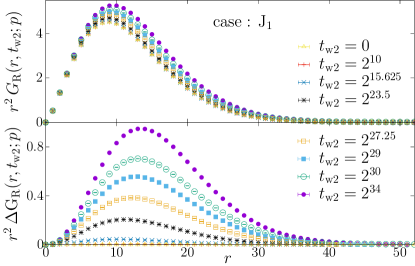
Figure 3: Numerical construction of a memory coefficient. Top: the curves $r^{2}G_{\mathrm{R}}(r,t_{\mathrm{w2}};p)$ vs. $r$ show small, but detectable, differences as $t_{\mathrm{w2}}$ varies, for temperature cycles built from the $T$-drop J₁ in Table 2 ($t_{\mathrm{w1}}=2^{19.5}$). Bottom: as in Top, but subtracting the native $G_{\mathrm{R}}$ from the correlation function of the temperature-cycled system, see Eq. (6). As the time spent at the colder temperature $T_{2}$ increases, the system loses memory. The memory loss is evinced by the increasing signal in $r^{2}\Delta G_{\mathrm{R}}$.

Fig. 3-top exhibits a small but detectable difference in the behavior of $r^{2}G_{\mathrm{R}}$ as $t_{\mathrm{w2}}$ varies in cycles built from $T$-drop $J_{1}$ in Table 2. This success has encouraged to consider the curve with $t_{\mathrm{w2}}=0$ as the reference curve . We evaluate effects due to $t_{\mathrm{w2}}$ as

$$\Delta G_{\mathrm{R}}(r,t_{\mathrm{w2}};p)=G_{\mathrm{R}}(r,t_{\mathrm{w2}};p)-G_{\mathrm{R}}(r,0;p)\,.$$ (6)

The difference in the correlation lengths in Eq. (6) represents the amount of growth in the correlation length that has occurred at $T_{2}$ for a waiting time $t_{\mathrm{w2}}$. If the temperature difference $T_{1}-T_{2}$ is sufficient for full chaos to develop at $T_{2}$, then $\Delta G_{\text{R}}(r,t_{\mathrm{w2}};T_{1})$ represents the competing correlation length that interferes with the native correlation length established at $T_{1}$.

From Fig. 3–bottom, it is natural to define the numerical memory coefficient $\mathcal{C}_{\mathrm{num}}$ as

$$\mathcal{C}_{\mathrm{num}}=1-\frac{\int_{0}^{\infty}\mathrm{d}r\,r^{2}\,\Delta G_{\text{R}}(r,t_{\mathrm{w2}};p)}{\int_{0}^{\infty}\mathrm{d}r\,r^{2}\,G_{\text{R}}(r,0;p)}\,.$$ (7)

Further scaling arguments supporting our choice can be found in Appendix C. Our results for $\mathcal{C}_{\mathrm{num}}$ are presented in Fig. 1, for several temperature cycles built from the temperature drops in Table  2. The values of $T_{1}$, $T_{2}$ and $t_{\mathrm{w1}}$ were chosen to meet the chaos requirement proposed in Zhai et al. (2022); Baity-Jesi et al. (2023) (the only exception is $\mathrm{J}_{9}$, used as a testing case for the scaling analysis, below). It is comforting that, even when the ratio $t_{\mathrm{w2}}/t_{\mathrm{w1}}$ is as large as in Fig. 3, we still obtain $\mathcal{C}_{\mathrm{num}}>0.75$.

Discussion.

Memory can be quantified in several ways: we have proposed two such memory coefficients, $\mathcal{C}_{\text{Zeeman}}$ and $\mathcal{C}_{\text{num}}$, respectively, adapted to experimental and numerical computation. Each coefficient is used in a different time scale, see Fig. 1. Furthermore, Freedberg et al. (2023) proposes yet another experimental coefficient, $\mathcal{C}_{\chi^{\prime\prime}}$, based on the linear response to a magnetic field (rather than the nonlinear responses considered herein). It is obvious that more options exist. Hence, it is natural to ask what (if any) is the relationship between these coefficients.

We look for this relationship in the two length scales that rule our nonequilibrium dynamics, namely ${\zeta^{\mathrm{jump}}(T_{2},t_{\mathrm{w2}})}$ and ${\xi_{\mathrm{micro}}^{\mathrm{native}}(T_{1},t_{\mathrm{w1}})}$. If we succeed in expressing our coefficients as simple functions of these two lengths, we shall have a natural bridge between different memory definitions.

Specifically, we consider two variables $x$ and $y$:

$$x\!=\!\left[\frac{\zeta^{\mathrm{jump}}(T_{2},t_{\mathrm{w2}})}{\xi_{\mathrm{micro}}^{\mathrm{native}}(T_{1},t_{\mathrm{w1}})}\right]^{D-\tfrac{\theta}{2}}\!\!,\ y=\frac{T_{1}}{T_{\mathrm{g}}}\,\zeta^{\mathrm{jump}}(T_{2},t_{\mathrm{w2}})\,.$$ (8)

Both scaling variables, $x$ and $y$, are approximately accessible to experiment through Eqs. (1) and (2); we shall name their experimental proxies $x^{\prime}$ and $y^{\prime}$ . Therefore, we seek numerical constants $a_{1}$ and $a_{2}$, [see Appendix  E for details], such that the $\mathcal{C}_{\mathrm{num}}$ from all our temperature cycles fall onto a single function of

$$\mathcal{F}(x,y)=y\,[1+a_{1}x+a_{2}x^{2}]\,.$$ (9)

Setting aside $T$-drop J₉, which does not meet the chaos condition, the overall linear behavior in Fig. 4–bottom is reassuring.

With appropriate $a^{\prime}_{1}$ and $a^{\prime}_{2}$ in Eq. (9), see Appendix E, the data for $\mathcal{C}_{\chi^{\prime\prime}}$ Freedberg et al. (2023) also fall onto a smooth function of $\mathcal{F}^{\prime}(x^{\prime},y^{\prime})$, Fig. 4–top. There is a problem, however: $\mathcal{C}_{\chi^{\prime\prime}}$ goes to one for $t_{\mathrm{w2}}$ significantly larger than zero ($\mathcal{F^{\prime}}=0$ only at $t_{\mathrm{w2}}=0$). The same problem afflicts $\mathcal{C}_{\mathrm{num}}$, albeit to a lesser degree. Interestingly, when plotted as a function of $\mathcal{F}^{\prime}$, $\mathcal{C}_{\mathrm{Zeeman}}$ is compatible with a straight line that goes through $\mathcal{C}=1$ at $\mathcal{F}^{\prime}=0$, as it should. So, at least in this respect, $\mathcal{C}_{\mathrm{Zeeman}}$ is the most sensible coefficient.

Perhaps more importantly, the scaling representation (dashed line in Fig. 4–top) evinces that, away from the $\mathcal{C}\approx 1$ region, the relation $\mathcal{C}_{\chi^{\prime\prime}}\approx[\mathcal{C}_{\text{Zeeman}}]^{K}$ holds with $K\approx 3.9$. This relation makes it obvious that the different memory coefficients carry the same physical information.

In summary, we have identified the length scales that govern memory in spin glasses in the form of a simple scaling law. We expect this picture to carry over to other glassy systems that exhibit rejuvenation and memory.

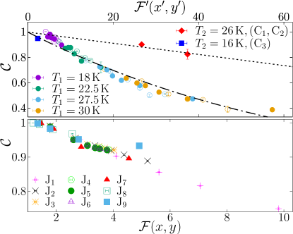
Figure 4: Top: Experimental memory coefficients $\mathcal{C}_{\chi^{\prime\prime}}$ (circles, data from  Freedberg et al. (2023); $T_{1}=T_{2}+4$ K) and $\mathcal{C}_{\mathrm{Zeeman}}$ (rhombus and squares, see Table 1) versus the scaling function in Eq. (9). See text for the computation of the $x^{\prime}$ and $y^{\prime}$ proxies. Empty circles refer to $t_{\mathrm{w1}}=1\,\mathrm{h}$ (full circles for $t_{\mathrm{w2}}=3\,\mathrm{h})$. The dotted line is a fit to a straight $\mathcal{C}_{\mathrm{Zeeman}}=1-\alpha\mathcal{F}^{\prime}$. The dashed line is $(1-\alpha\mathcal{F}^{\prime})^{3.9}$ and represents the experimental findings for $\mathcal{C}_{\chi^{\prime\prime}}$ surprisingly well. Bottom: As in Top, for memory coefficient $\mathcal{C}_{\mathrm{num}}$ [$x$ and $y$ are given in Eq. (8)], see Table 2 for details.

Appendix A Our simulations on Janus II

We simulate the Edwards-Anderson model in a cubic lattice with linear size $L=160$ and periodic boundary conditions. The Ising spins $S_{\bm{x}}=\pm 1$ occupy the lattice nodes and interact with their nearest lattice-neighbors through the Hamiltonian

$$H=-\sum_{\langle\bm{x},\bm{y}\rangle}J_{\bm{x},\bm{y}}S_{\bm{x}}S_{\bm{y}}\,,$$ (10)

where the coupling constants are independent random variables that are fixed at the beginning of the simulation (we choose $J_{\bm{x},\bm{y}}=\pm 1$ with 50% probability). A choice of the $\{J_{\bm{x},\bm{y}}\}$ is named a sample. The model in Eq. (10) undergoes a phase transition at temperature $T_{\mathrm{c}}=1.1019(29)$ Baity-Jesi et al. (2013), separating the paramagnetic phase (at high temperatures) from the spin-glass phase (at low temperatures).

We study the nonequilibrium dynamics of the model with a Metropolis algorithm. The time unit is a full lattice sweep (roughly corresponding to one picosecond of physical time Mydosh (1993)). The simulation is performed on the Janus II custom-built supercomputer Baity-Jesi et al. (2014)

We consider 16 statistically independent samples. For each sample, we simulate $N_{\text{R}}=512$ independent replicas (i.e., $N_{\text{R}}$ system copies that share the couplings $\{J_{\bm{x},\bm{y}}\}$ but are otherwise statistically independent). Replicas are employed to compute correlation functions as explained in Refs. Zhai et al. (2020); Paga et al. (2021); Baity-Jesi et al. (2023)

Appendix B A simple relation between coherence lengths

In this section we define the relevant length scales, $\xi_{\mathrm{micro}}$, $\zeta$ and $\xi_{\mathrm{Zeeman}}$ and their relationships:

• $\xi_{\mathrm{micro}}(t_{\mathrm{w}})$ is the size of the glassy domain. It is estimated through the replicon propagator, $G_{\mathrm{R}}(r,t_{\mathrm{w}};p)$.

• $\xi_{\mathrm{Zeeman}}$ is obtained by counting the number of spins that react coherently to an external magnetic field, and thereby the volume of correlated spins subtended by the correlation length $\xi_{\mathrm{Zeeman}}$. This is the only experimentally accessible method for obtaining a correlation length directly.

• $\zeta(t_{1},t_{2})$ is the scale at which defects are correlated .

In a fixed-temperature protocol, these quantities are almost equivalent Zhai et al. (2020); Paga et al. (2021); Baity-Jesi et al. (2023). The scenario is more intricate in varying-temperature protocols because of temperature chaos. In Fig. 5, we compare these length scales in varying-temperature protocols.

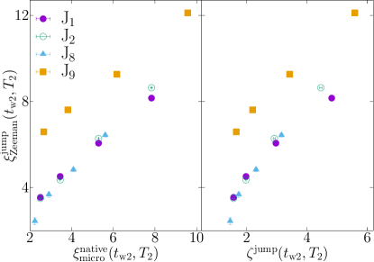
Figure 5: Comparison between correlation lengths. Left: we compare the behavior of the effective correlation length, $\xi_{\mathrm{Zeeman}}$, as a function of the microscopic correlation length, $\xi_{\mathrm{micro}}^{\mathrm{native}}(t_{\mathrm{w2}},T_{2})$ evaluated at a fixed-temperature. Right, we show the behavior of $\xi_{\mathrm{Zeeman}}$ as a function of the coherence scale $\zeta(t_{\mathrm{w2}},T_{2})$ calculated for varying-temperatures. The ${\text{J}}_{n}$ temperature cycles and related wait times $t_{\mathrm{w1}}$ are listed in Table II in the main text.

As the reader can notice, if chaos is large [${\text{J}}_{1}$, ${\text{J}}_{2}$ and ${\text{J}}_{8}$], an equivalence exists between $\xi_{\mathrm{Zeeman}}$, $\zeta$, and $\xi_{\mathrm{micro}}$. Otherwise [${\text{J}}_{9}$], the number of correlated spins is not a good proxy for $\zeta$.

Appendix C Scaling of $\chi^{\prime}$, $\chi^{\prime\prime}$ and ${\chi}_{2}/V$

In this section, we show that the dynamical behavior of the three susceptibilities, $\chi^{\prime}$, $\chi^{\prime\prime}$ and $\hat{\chi}_{2}\equiv\chi_{2}/V$, are similar. The former two are measured in conventional memory experiments (e.g., in Ref. Freedberg et al. (2023)), and the latter in numerical simulations.

We analyze first the scaling properties near the critical point. We then extend the analysis to the glass phase.

In the following we use $\epsilon\equiv(T-T_{\mathrm{g}})/T_{\mathrm{g}}$ to denote the reduced temperature.

On the one hand, the experimentally computed linear magnetic susceptibilities behave as Nordblad and Svedlindh (1997)

$$\begin{split}\frac{\chi_{0}-\chi^{\prime}}{\chi_{0}}&\sim\epsilon^{\beta}G(t/\tau)\,,\\ \chi^{\prime\prime}&\sim\epsilon^{\beta}H(t/\tau)\,,\end{split}$$ (11)

where we have taken both linear magnetic susceptibilities in the time domain (the relationship to frequency is a simple Fourier transform). Above, $G(\cdot)$ and $H(\cdot)$ are two scaling functions, and $\chi_{0}$ is the equilibrium value of the linear magnetic susceptibility at the critical point.

On the other hand, the nonlinear spin-glass susceptibility per spin, computed in numerical simulations, scales as Nordblad and Svedlindh (1997)

$${\hat{\chi}}_{2}\sim\epsilon^{2\beta}K(t/\tau)\,,$$ (12)

with a suitable scaling function $K(\cdot)$. At the critical point, there is only a critical mode and we can avoid the use of the replicon term.

The rationale behind these scaling relations is that the overlap is essentially the magnetization squared. The linear magnetic susceptibilities scale with the exponent associated with the average of the overlap $q$ (the fluctuation of the magnetization is given by $\langle m^{2}\rangle$, the average of the overlap), and $\chi_{2}$ is a nonlinear susceptibility per spin associated with the overlap. Therefore, it scales with the usual exponent $\gamma=2\beta-\nu D$. Remember that the order parameter, the overlap, scales with the exponent $\beta$ and that $\hat{\chi}_{2}=\chi_{2}/V$.

For the analogous scaling relations in the spin-glass phase, the out-of-equilibrium situation is dominated by the replicon mode. The only diverging nonlinear susceptibility is the replicon nonlinear one, defined as

$$\chi_{2}(t)=\int_{0}^{\infty}dr\,r^{2}\,G_{\mathrm{R}}(r,t)\,.$$ (13)

The overlap field scales with the replicon exponent $\theta$ as $q\sim\xi^{-\theta/2}$ (see Appendix H of Fernandez et al. (2022)), so we can write the dependence of these susceptibilities on the correlation length as

$$\begin{split}\frac{\chi_{0}-\chi^{\prime}}{\chi_{0}}&\sim\chi^{\prime\prime}\sim\xi(t)^{-\theta/2}\,,\\ {\hat{\chi}}_{2}&\sim\xi(t)^{-\theta}\,.\end{split}$$ (14)

We conclude from this analysis that the dynamical behaviors of these different susceptibilities are similar. Hence, we can safely compare the results from numerical simulations with experiments that measure $\chi^{\prime\prime}$ Freedberg et al. (2023) for this reason.

Appendix D Experimental details and data processing

This section explores the experimental protocol for measuring the change in magnetization as a function of $\log t$. In particular, it delves into the nuances of data processing for accurate identification of the time that the dynamic function $S(t)$ peaks, $t_{\mathrm{w}}^{\text{eff}}(H)$. As discussed in the main body of the text, the accurate determination of $t_{\mathrm{w}}^{\text{eff}}(H)$ is vital for extracting $\xi_{\text{Zeeman}}$.

Magnetization measurements were conducted using a Quantum Design MPMS system. The magnetization was gauged as the sample traversed through an array of superconducting quantum interference devices (SQUIDs). The system was set to take continuous magnetization measurements over approximately 10 hours for $t_{\mathrm{w}}=1$ h, and 30 hours for $t_{\mathrm{w}}=3$ h.

The magnetization as a function of time $t$ displayed intermittent spikes owing to the SQUIDs’ measurements. A representative example is exhibited in Figure 6. These aberrations, typically because of external interference with the SQUID coil, were subsequently removed in our analysis. The first derivative of the magnetization as a function of $\log t$ was then calculated.

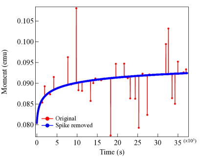
Figure 6: Raw measurement data and the spike removed data Data from a typical $S(t)$ measurement. (Red) The raw magnetization vs $t$ with random spikes from the SQUID measurements. (Blue) Magnetization vs $t$ with spikes removed.

The derivative of the raw data tends to be noisy, complicating the task of identifying the position of the peak in $S(t)$. It was necessary to suitably smooth the $S(t)$ curve. We utilized a Chebyshev polynomial fit for the $M$ vs $t$ curve prior to computing its derivative.

With an appropriate number of terms, the Chebyshev polynomial fit accurately represents the raw $M$ vs $t$ data, effectively eliminating the spikes in the ${\mathrm{d}}M/{\mathrm{d}}\log t$ data produced by measurement artifacts, as illustrated in Figure 7. A 60-term Chebyshev polynomial fit typically depicts the $S(t)$ curve satisfactorily, with less than a 1% residual. Using higher terms further reduces this residual. The Chebyshev polynomial fit excels over a simple box smoothing of raw data because it preserves the spline of the $M$ vs $t$ curve while simultaneously decreasing the noise in the derivative.

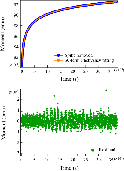
Figure 7: Chebyshev polynomial fitting of the data and the residual (Top) The spike removed $M$ vs $t$ data with 60-term Chebsyhev fit of the data marked in orange. (Bottom) The residual of the Chebyshev fit.

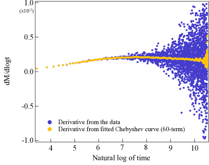
Figure 8: Comparison of the derivative of the raw data vs the derivative of one Chebyshev fitted curve. (Blue) The ${\mathrm{d}}M/{\mathrm{d}}\log t$ plot of raw magnetization vs $\log t$. (Yellow) The ${\mathrm{d}}M/{\mathrm{d}}\log t$ plot of a 60-term Chebyshev fit of the magnetization vs $\log t$.

Upon obtaining the derivative of the Chebyshev polynomial, we constructed a single Lorentzian peak function with a constant background:

$$\begin{split}f(x)=\frac{A\gamma^{2}}{(x-x_{0})^{2}+\gamma^{2}}+C~{}~{}.\end{split}$$ (15)

In this equation, $A$ denotes the amplitude of the peak, $x_{0}$ represents the center, and $\gamma$ indicates the peak width. As depicted in Figure 8, the derivative of the Chebyshev curve provides a relatively uncluttered peak with a fit to a Lorentzian shape. With a sufficient number of Chebyshev polynomial terms, the fitted curve can trace the raw data precisely.

To ensure that the Chebyshev polynomial accurately represents the $M$ vs $t$ data, we iteratively conducted the fitting and peak searching procedure over a number range of terms, typically from 30 to 1200. Each iteration produced a value for the time at which the Lorentzian peaks. We then calculated the average of these values to determine the peak time for a given $S(t)$ measurement. The error bar for the time of the peak was determined from the standard deviation of the peak times. In cases where overfitting or underfitting was apparent within certain ranges of the number of Chebyshev polynomial terms, as evinced by deviant peak values, the peak values obtained in these ranges were disregarded.

Appendix E Determination of the coefficients for the scaling function $\mathcal{F}(x,y)$

As we have explained in the main text, we introduce a simple scaling function $\mathcal{F}(x,y)$ for describing both the experimental and numerical data. Here we report the details for the determination of the constants $a_{1}$ and $a_{2}$ [and analogously $a_{1}^{\prime}$ and $a_{2}^{\prime}$].
Our procedure consists of two steps:

• we fit the data for the memory coefficient under consideration —$\mathcal{C}_{\text{num}}$ or $\mathcal{C}_{\chi^{\prime\prime}}$— to a smooth, generic function of the scaling function $\mathcal{F}(x,y)$ introduced in the main text:

  $$\mathcal{C}(x,y)=B_{0}-B_{1}\,\mathcal{F}(x,y)-B_{2}[\mathcal{F}(x,y)]^{2},$$ (16)

  Note that there are five fit parameters, namely $B_{0}$, $B_{1}$ and $B_{2}$ and the two parameters $a_{1}$ and $a_{2}$ that determine $\mathcal{F}(x,y)$.

• The free parameters $B_{0},B_{1},B_{2}$ are disregarded in the analysis. Instead, we keep $a_{1},a_{2}$ (or $a_{1}^{\prime}$ and $a_{2}^{\prime}$ for $\mathcal{C}_{\chi^{\prime\prime}}$), to describe our data as a function of the scaling function $\mathcal{F}(x,y)$ [$\mathcal{F}^{\prime}(x^{\prime},y^{\prime})$ in the case of $\mathcal{C}_{\chi^{\prime\prime}}$].

For the numerical data, $B_{0}\simeq 1$ and $B_{2}=0$. The data for $\mathcal{C}_{\chi^{\prime\prime}}$, taken from Ref. Freedberg et al. (2023), require $B_{2}\neq 0$.

References

- Keim et al. (2019) N. C. Keim, J. D. Paulsen, Z. Zeravcic, S. Sastry, and S. R. Nagel, Rev. Mod. Phys. 91, 035002 (2019).
- Bandi et al. (2018) M. M. Bandi, H. G. E. Hentschel, I. Procaccia, S. Roy, and J. Zylberg, Europhys. Lett. 122, 38003 (2018).
- Koide et al. (2006) T. Koide, G. Krein, and R. O. Ramos, Phys. Lett. B 636, 96 (2006).
- Ozon et al. (2003) F. Ozon, T. Narita, A. Knaebel, P. Debrégeas, Hébraud, and J.-P. Munch, Phys. Rev. E 68, 032401 (2003).
- Bellon et al. (2000) L. Bellon, S. Ciliberto, and C. Laroche, Europhys. Lett. 51, 551 (2000).
- Yardimci and Leheny (2003) H. Yardimci and R. L. Leheny, Europhys. Lett. 62, 203 (2003).
- Bouchaud et al. (2001) J.-P. Bouchaud, P. Doussineau, T. de Lacerda-Arôso, and A. Levelut, Eur. Phys. J. B 21, 335 (2001).
- Mueller and Shchur (2004) V. Mueller and Y. Shchur, Europhys. Lett. 65, 137 (2004).
- Scalliet and Berthier (2019) C. Scalliet and L. Berthier, Phys. Rev. Lett. 122, 255502 (2019).
- Pashine et al. (2019) N. Pashine, D. Hexner, A. J. Liu, and S. R. Nagel, Science Advances 5, eaax4215 (2019), https://www.science.org/doi/pdf/10.1126/sciadv.aax4215 .
- Lefloch et al. (1992) F. Lefloch, J. Hammann, M. Ocio, and E. Vincent, EPL (Europhysics Letters) 18, 647 (1992).
- Jonason et al. (1998) K. Jonason, E. Vincent, J. Hammann, J. P. Bouchaud, and P. Nordblad, Phys. Rev. Lett. 81, 3243 (1998).
- Lundgren et al. (1983) L. Lundgren, P. Svedlindh, and O. Beckman, J. Magn. Magn. Mater. 31–34, 1349 (1983).
- Jonsson et al. (1999) T. Jonsson, K. Jonason, P. E. Jönsson, and P. Nordblad, Phys. Rev. B 59, 8770 (1999).
- Hammann et al. (2000) J. Hammann, E. Vincent, V. Dupuis, M. Alba, M. Ocio, and J.-P. Bouchaud, J. Phys. Soc. Jpn. , Suppl A. 206 (2000).
- Vincent (2007) E. Vincent, in Ageing and the Glass Transition, Lecture Notes in Physics No. 716, edited by M. Henkel, M. Pleimling, and R. Sanctuary (Springer, 2007).
- Vincent (2023) E. Vincent, “Spin glass experiments,” (2023), to appear in Elsevier Encyclopedia of Condensed Matter Physics, 2nd ed., arXiv:2208.00981 .
- Zhai et al. (2019) Q. Zhai, V. Martin-Mayor, D. L. Schlagel, G. G. Kenning, and R. L. Orbach, Phys. Rev. B 100, 094202 (2019).
- Zhai et al. (2020) Q. Zhai, I. Paga, M. Baity-Jesi, E. Calore, A. Cruz, L. A. Fernandez, J. M. Gil-Narvion, I. Gonzalez-Adalid Pemartin, A. Gordillo-Guerrero, D. Iñiguez, A. Maiorano, E. Marinari, V. Martin-Mayor, J. Moreno-Gordo, A. Muñoz Sudupe, D. Navarro, R. L. Orbach, G. Parisi, S. Perez-Gaviro, F. Ricci-Tersenghi, J. J. Ruiz-Lorenzo, S. F. Schifano, D. L. Schlagel, B. Seoane, A. Tarancon, R. Tripiccione, and D. Yllanes, Phys. Rev. Lett. 125, 237202 (2020).
- Paga et al. (2021) I. Paga, Q. Zhai, M. Baity-Jesi, E. Calore, A. Cruz, L. A. Fernandez, J. M. Gil-Narvion, I. Gonzalez-Adalid Pemartin, A. Gordillo-Guerrero, D. Iñiguez, A. Maiorano, E. Marinari, V. Martin-Mayor, J. Moreno-Gordo, A. Muñoz-Sudupe, D. Navarro, R. L. Orbach, G. Parisi, S. Perez-Gaviro, F. Ricci-Tersenghi, J. J. Ruiz-Lorenzo, S. F. Schifano, D. L. Schlagel, B. Seoane, A. Tarancon, R. Tripiccione, and D. Yllanes, Journal of Statistical Mechanics: Theory and Experiment 2021, 033301 (2021).
- Baity-Jesi et al. (2018) M. Baity-Jesi, E. Calore, A. Cruz, L. A. Fernandez, J. M. Gil-Narvion, A. Gordillo-Guerrero, D. Iñiguez, A. Maiorano, E. Marinari, V. Martin-Mayor, J. Moreno-Gordo, A. Muñoz Sudupe, D. Navarro, G. Parisi, S. Perez-Gaviro, F. Ricci-Tersenghi, J. J. Ruiz-Lorenzo, S. F. Schifano, B. Seoane, A. Tarancon, R. Tripiccione, and D. Yllanes (Janus Collaboration), Phys. Rev. Lett. 120, 267203 (2018).
- Baity-Jesi et al. (2021) M. Baity-Jesi, E. Calore, A. Cruz, L. A. Fernandez, J. M. Gil-Narvion, I. Gonzalez-Adalid Pemartin, A. Gordillo-Guerrero, D. Iñiguez, A. Maiorano, E. Marinari, V. Martin-Mayor, J. Moreno-Gordo, A. Muñoz Sudupe, D. Navarro, I. Paga, G. Parisi, S. Perez-Gaviro, F. Ricci-Tersenghi, J. J. Ruiz-Lorenzo, S. F. Schifano, B. Seoane, A. Tarancon, R. Tripiccione, and D. Yllanes, Communications physics 4, 74 (2021), https://www.nature.com/articles/s42005-021-00565-9.pdf .
- Zhai et al. (2022) Q. Zhai, R. L. Orbach, and D. L. Schlagel, Phys. Rev. B 105, 014434 (2022).
- Komori et al. (2000) T. Komori, H. Yoshino, and H. Takayama, Journal of the Physical Society of Japan 69, 1192 (2000), arXiv:cond-mat/9908078 .
- Picco et al. (2001) M. Picco, F. Ricci-Tersenghi, and F. Ritort, Phys. Rev. B 63, 174412 (2001).
- Berthier and Bouchaud (2002) L. Berthier and J.-P. Bouchaud, Phys. Rev. B 66, 054404 (2002).
- Takayama and Hukushima (2002) H. Takayama and K. Hukushima, Journal of the Physical Society of Japan 71, 3003 (2002).
- Maiorano et al. (2005) A. Maiorano, E. Marinari, and F. Ricci-Tersenghi, Phys. Rev. B 72, 104411 (2005).
- Jiménez et al. (2005) S. Jiménez, V. Martín-Mayor, and S. Pérez-Gaviro, Phys. Rev. B 72, 054417 (2005).
- Baity-Jesi et al. (2023) M. Baity-Jesi, E. Calore, A. Cruz, L. A. Fernandez, J. M. Gil-Narvion, I. Gonzalez-Adalid Pemartin, A. Gordillo-Guerrero, D. Iñiguez, A. Maiorano, E. Marinari, V. Martin-Mayor, J. Moreno-Gordo, A. Muñoz Sudupe, D. Navarro, I. Paga, G. Parisi, S. Perez-Gaviro, F. Ricci-Tersenghi, J. J. Ruiz-Lorenzo, S. F. Schifano, B. Seoane, A. Tarancon, and D. Yllanes, Nat. Phys. (2023), https://doi.org/10.1038/s41567-023-02014-6, arXiv:2207.06207 .
- Baity-Jesi et al. (2014) M. Baity-Jesi, R. A. Baños, A. Cruz, L. A. Fernandez, J. M. Gil-Narvion, A. Gordillo-Guerrero, D. Iniguez, A. Maiorano, F. Mantovani, E. Marinari, V. Martín-Mayor, J. Monforte-Garcia, A. Muñoz Sudupe, D. Navarro, G. Parisi, S. Perez-Gaviro, M. Pivanti, F. Ricci-Tersenghi, J. J. Ruiz-Lorenzo, S. F. Schifano, B. Seoane, A. Tarancon, R. Tripiccione, and D. Yllanes (Janus Collaboration), Comp. Phys. Comm 185, 550 (2014), arXiv:1310.1032 .
- Fernandez et al. (2013) L. A. Fernandez, V. Martín-Mayor, G. Parisi, and B. Seoane, EPL 103, 67003 (2013), arXiv:1307.2361 .
- Fernández et al. (2016) L. A. Fernández, E. Marinari, V. Martín-Mayor, G. Parisi, and D. Yllanes, Journal of Statistical Mechanics: Theory and Experiment 2016, 123301 (2016), arXiv:1605.03025 .
- Billoire et al. (2018) A. Billoire, L. A. Fernandez, A. Maiorano, E. Marinari, V. Martin-Mayor, J. Moreno-Gordo, G. Parisi, F. Ricci-Tersenghi, and J. J. Ruiz-Lorenzo, Journal of Statistical Mechanics: Theory and Experiment 2018, 033302 (2018).
- Freedberg et al. (2023) J. Freedberg, W. J. Meese, J. He, D. L. Schlagel, E. D. Dahlberg, and R. L. Orbach, “On the nature of memory and rejuvenation in glassy systems,” (2023), arXiv:2305.17296 [cond-mat.dis-nn] .
- Paga et al. (2023) I. Paga, Q. Zhai, M. Baity-Jesi, E. Calore, A. Cruz, C. Cummings, L. A. Fernandez, J. M. Gil-Narvion, I. G.-A. Pemartin, A. Gordillo-Guerrero, D. Iñiguez, G. G. Kenning, A. Maiorano, E. Marinari, V. Martin-Mayor, J. Moreno-Gordo, A. Muñoz Sudupe, D. Navarro, R. L. Orbach, G. Parisi, S. Perez-Gaviro, F. Ricci-Tersenghi, J. J. Ruiz-Lorenzo, S. F. Schifano, D. L. Schlagel, B. Seoane, A. Tarancon, and D. Yllanes, Phys. Rev. B 107, 214436 (2023).
- Joh et al. (1999) Y. G. Joh, R. Orbach, G. G. Wood, J. Hammann, and E. Vincent, Phys. Rev. Lett. 82, 438 (1999).
- Belletti et al. (2008) F. Belletti, M. Cotallo, A. Cruz, L. A. Fernandez, A. Gordillo-Guerrero, M. Guidetti, A. Maiorano, F. Mantovani, E. Marinari, V. Martín-Mayor, A. M. Sudupe, D. Navarro, G. Parisi, S. Perez-Gaviro, J. J. Ruiz-Lorenzo, S. F. Schifano, D. Sciretti, A. Tarancon, R. Tripiccione, J. L. Velasco, and D. Yllanes (Janus Collaboration), Phys. Rev. Lett. 101, 157201 (2008), arXiv:0804.1471 .
- Belletti et al. (2009) F. Belletti, A. Cruz, L. A. Fernandez, A. Gordillo-Guerrero, M. Guidetti, A. Maiorano, F. Mantovani, E. Marinari, V. Martín-Mayor, J. Monforte, A. Muñoz Sudupe, D. Navarro, G. Parisi, S. Perez-Gaviro, J. J. Ruiz-Lorenzo, S. F. Schifano, D. Sciretti, A. Tarancon, R. Tripiccione, and D. Yllanes (Janus Collaboration), J. Stat. Phys. 135, 1121 (2009), arXiv:0811.2864 .
- Baity-Jesi et al. (2017a) M. Baity-Jesi, E. Calore, A. Cruz, L. A. Fernandez, J. M. Gil-Narvión, A. Gordillo-Guerrero, D. Iñiguez, A. Maiorano, E. Marinari, V. Martin-Mayor, J. Monforte-Garcia, A. Muñoz Sudupe, D. Navarro, G. Parisi, S. Perez-Gaviro, F. Ricci-Tersenghi, J. J. Ruiz-Lorenzo, S. F. Schifano, B. Seoane, A. Tarancón, R. Tripiccione, and D. Yllanes, Proceedings of the National Academy of Sciences 114, 1838 (2017a).
- Paga et al. (2022) I. Paga, Q. Zhai, M. Baity-Jesi, E. Calore, A. Cruz, C. Cummings, L. A. Fernandez, J. M. Gil-Narvion, I. G.-A. Pemartin, A. Gordillo-Guerrero, D. Iñiguez, G. G. Kenning, A. Maiorano, E. Marinari, V. Martin-Mayor, J. Moreno-Gordo, A. Muñoz-Sudupe, D. Navarro, R. L. Orbach, G. Parisi, S. Perez-Gaviro, F. Ricci-Tersenghi, J. J. Ruiz-Lorenzo, S. F. Schifano, D. L. Schlagel, B. Seoane, A. Tarancon, and D. Yllanes, “Magnetic-field symmetry breaking in spin glasses,” (2022), arXiv:2207.10640 [cond-mat.dis-nn] .
- Note (1) Our simulations will closely follow (Baity-Jesi et al., 2023) (for the sake of completeness we describe them in Table 2 and Appendix A).
- Note (2) Due to rotational invariance Belletti et al. (2009), essentially depends on .
- Baity-Jesi et al. (2017b) M. Baity-Jesi, E. Calore, A. Cruz, L. A. Fernandez, J. M. Gil-Narvion, A. Gordillo-Guerrero, D. Iñiguez, A. Maiorano, E. Marinari, V. Martin-Mayor, J. Monforte-Garcia, A. Muñoz Sudupe, D. Navarro, G. Parisi, S. Perez-Gaviro, F. Ricci-Tersenghi, J. J. Ruiz-Lorenzo, S. F. Schifano, B. Seoane, A. Tarancon, R. Tripiccione, and D. Yllanes (Janus Collaboration), Phys. Rev. Lett. 118, 157202 (2017b).
- Note (3) A native protocol can be regarded as a cycle with ( is indistinguishable from within our numerical accuracy for native runs).
- Note (4) We computed and from the approximation (Baity-Jesi et al., 2023) and the approximate law with and \tmspace+.1667emps Zhai et al. (2019). Indeed, our measurements of in Table 1 rather follow . We omit the constant background to diminish corrections to scaling.
- Baity-Jesi et al. (2013) M. Baity-Jesi, R. A. Baños, A. Cruz, L. A. Fernandez, J. M. Gil-Narvion, A. Gordillo-Guerrero, D. Iniguez, A. Maiorano, F. Mantovani, E. Marinari, V. Martín-Mayor, J. Monforte-Garcia, A. Muñoz Sudupe, D. Navarro, G. Parisi, S. Perez-Gaviro, M. Pivanti, F. Ricci-Tersenghi, J. J. Ruiz-Lorenzo, S. F. Schifano, B. Seoane, A. Tarancon, R. Tripiccione, and D. Yllanes (Janus Collaboration), Phys. Rev. B 88, 224416 (2013), arXiv:1310.2910 .
- Mydosh (1993) J. A. Mydosh, Spin Glasses: an Experimental Introduction (Taylor and Francis, London, 1993).
- Note (5) See Refs. Belletti et al. (2008); Baity-Jesi et al. (2023) for more details.
- Nordblad and Svedlindh (1997) P. Nordblad and P. Svedlindh, Experiments on Spin Glasses (World Scientific, Singapore, 1997) spin Glasses and Random Fields edited by A.P. Young, Directions in Condensed Matter Physics Vol. 12, p. 1.
- Fernandez et al. (2022) L. A. Fernandez, I. Gonzalez-Adalid Pemartin, V. Martin-Mayor, G. Parisi, F. Ricci-Tersenghi, T. Rizzo, J. J. Ruiz-Lorenzo, and M. Veca, Phys. Rev. E 105, 054106 (2022).
- Note (6) We employ for and for .