Resurgent Structure of the Topological String and the First Painlevé Equation

Abstract.

We present an explicit formula for the Stokes automorphism acting on the topological string partition function. When written in terms of the dual partition function, our formula implies that flat coordinates in topological string theory transform as quantum periods, and according to the Delabaere–Dillinger–Pham formula. We first show how the formula follows from the non-linear Stokes phenomenon of the Painlevé I equation, together with the connection between its $\tau$-function and topological strings on elliptic curves. Then, we show that this formula is also a consequence of a recent conjecture on the resurgent structure of the topological string, based on the holomorphic anomaly equations, and it is in fact valid for arbitrary Calabi–Yau threefolds.

1. Introduction and conclusions

Topological string theory has been at the center of many developments in modern mathematical physics. For example, through string dualities [DV02, BKMnP09] and the topological recursion of [EO07] it is related to matrix models and the $1/N$ expansion. It has been also shown that certain “dual" partition functions appearing in topological string theory are closely related to $\tau$-functions of Painlevé equations [Iwa20, EGF21, MO22, EGFMO21]. These results have a close relation with the pioneering works [GIL12, BLM⁺17].

The basic quantities in topological string theory are given by formal perturbative series in the string coupling constant $g_{s}$, which are factorially divergent. One can then ask, in the spirit of the theory of resurgence [Éca81, MS16], what is the resurgent structure of these series, i.e. what are the exponentially small trans-series associated to their Borel singularities, and the associated Stokes constants. This question has been recently addressed in various works. Based on the trans-series approach of [CSESV16, CSESV15, CSMnS17], a conjecture for the resurgent structure of topological string theory on arbitrary Calabi–Yau (CY) threefolds was put forward in [GMn22a, GKPKMn23]. Although topological strings are closely related to quantum periods (also known as Voros symbols), their resurgent structure is quite different. For example, it is expected that the Stokes automorphisms of quantum periods are given by the Delabaere–Dillinger–Pham (DDP) formula [DDP93, DDP97, DP99] (see [GMn22b, DML22] for recent arguments in that direction), but the Stokes automorphisms act on the topological string partition function with a more complicated structure, and no closed formula is known for them.

In this paper we provide such a closed formula. It reads

$$\boxed{{\mathfrak{S}}Z(\nu;g_{s})=\exp\left\{a{\rm Li}_{2}\left({\rm e}^{-g_{s}\partial}\right)-g_{s}a\log\left(1-{\rm e}^{-g_{s}\partial}\right)\partial\right\}Z(\nu;g_{s})}$$ (1)

where $a$ is a Stokes constant, $\nu$ is the flat coordinate (or period) parametrizing the moduli space, and $\partial$ is the derivative w.r.t. $\nu$.

Although the partition function transforms in a relatively complicated way under a Stokes automorphism, the dual partition function (obtained from the original one after a discrete Fourier transform) transforms in a very simple way:

$$\boxed{{\mathfrak{S}}\tau(\nu,\rho;g_{s})={\rm e}^{a{\rm Li}_{2}({\rm e}^{2\pi{\rm i}\rho/g_{s}})}\tau\left(\nu-ag_{s}\log(1-{\rm e}^{2\pi{\rm i}\rho/g_{s}}),\rho;g_{s}\right)}$$ (2)

i.e. it picks a prefactor involving the dilogarithm function, and its argument transforms indeed as a quantum period, following the DDP formula!

In this paper we give two lines of argument that lead to (1) and (2). The first one is based on the connection found in [Iwa20] between $\tau$-functions of the first Painlevé equation, and a dual partition function in topological string theory. By using this connection, one can show that the non-linear Stokes phenomenon of the first Painlevé equation leads to the above transformation formula for the dual partition function under a Stokes automorphism. Although this derivation is based on a particular example of the topological string partition function, the resulting formula turns out to be universally valid. To show this, we develop a second argument based on the conjectures for the resurgent structure of the topological string proposed in [GMn22a, GKPKMn23], and we provide a derivation of (1) in the spirit of alien calculus. Since the conjectures of [GMn22a, GKPKMn23] are valid for any topological string partition function which satisfies the holomorphic anomaly equations (HAE) of [BCOV94], we conclude that (1) applies universally to topological strings on arbitrary backgrounds.

As is mentioned above, the derivation based on [Iwa20] naturally relates the DDP formula to our main formula. The DDP formula has a close relationship with the BPS invariants in class ${\mathcal{S}}$ theories, which are defined by a weighted counting of saddle connections in the spectral network [GMN13a]. In fact, the DDP formula for the quantum period $V_{\mu}$ reads

$${\rm e}^{V_{\mu}}\mapsto{\rm e}^{V_{\mu}}(1+\sigma(\gamma){\rm e}^{V_{\gamma}})^{\Omega(\gamma)\langle\mu,\gamma\rangle},$$ (3)

where $\gamma$ is the cycle on the spectral curve associated with the saddle connection, $\sigma(\gamma)\in\{\pm 1\}$, and $\Omega(\gamma)$ is the BPS invariant; see e.g. [GMN13a, BS15]. In view of this, we expect the Stokes constant $a$ appearing in (1), (2) and in the formulae in section 3 to be given by a BPS invariant $\Omega(\gamma)$. The precise relation is

$$a={\Omega(\gamma)\over 2\pi{\rm i}}.$$ (4)

In the more general case considered in this paper, the $\Omega(\gamma)$ are given by the Donaldson–Thomas invariants of the CY threefold. Here, the cycle $\gamma$ is dual to the Borel singularity ${\mathcal{A}}$ underlying the Stokes discontinuity, and as we explain below ${\mathcal{A}}$ is an integral period of the CY geometry (up to an overall normalization). This identification between Stokes constants appearing in the resurgent structure of the topological string and BPS invariants was already suggested in [GMn22a, GKPKMn23], and it is also consistent with the results of [IK22, IK23]. Further evidence for this identification appears in the recent paper [Gu23].

We should mention that close cousins of (2) have appeared before in different, but related contexts. In [AP16] the transformation properties of a certain family of theta series defined on the (twistor space of the) hypermultiplet moduli space of CY threefolds under wall-crossing were studied. In the special case $k=1$, the theta series (1.5) in [AP16] reduces to the dual topological partition function [APP11], and their wall-crossing formula (1.9) agrees with our formula for the Stokes automorphism. In addition, for the formula to agree, one must have the relation (4), giving in this way additional evidence for the identification between Stokes constants and Donaldson–Thomas invariants. A detailed comparison between the wall-crossing formula of [AP16] and our formula will be made in section 3. A similar wall-crossing formula was also found in [CLT20] for the dual partition functions of some ${\mathcal{N}}=2$ gauge theories. Let us point out that in [AP16, APP11, CLT20] the transformation of the flat coordinate according to the DDP formula is essentially built in, while in our case it follows in a more indirect (and surprising) way from the resurgent structure of the topological string perturbative series. It would be very interesting to understand better the relation between [AP16, APP11, CLT20] and our approach.

The result obtained in this paper can be understood as relating the Stokes automorphism acting on the topological string partition function, to the Stokes automorphism acting on quantum periods. It might have a connection to the blowup formula which relates in a similar way the topological string free energy to the Nekrasov–Shatashvili free energy [GG19, JN20]. This idea has also been developed in [Gu23] and it might lead to a different derivation of our main formula. It would be also interesting to study the relation between our work and a series of papers by Bridgeland [Bri19, BM23, Bri23].

After this paper was finished, we were informed by R. Schiappa and M. Schwick that in forthcoming work [SST] they address similar issues and obtain related results, albeit with different methods.

Acknowledgements

We would like to thank Ioana Coman, Fabrizio del Monte, Alba Grassi, Paolo Gregori, Jie Gu, Shinobu Hosono, Omar Kidwai, Oleg Lisovyy, Pietro Longhi, Kento Osuga, Boris Pioline, Ricardo Schiappa, Masa-Hiko Saito, Maximilian Schwick, Atsushi Takahashi, Yoshitugu Takei and Joerg Teschner for useful conversations. We would also like to thank to Maxim Kontsevich and Yan Soibelman for organizing the IHES school “Wall-crossing structures, analyticity and resurgence," which made possible this collaboration. The work of K.I has been supported by the JSPS KAKENHI Grand Numbers 20K14323, 21K18576, 21H04994, 22H00094, 23K17654. The work of M.M. has been supported in part by the ERC-SyG project “Recursive and Exact New Quantum Theory" (ReNewQuantum), which received funding from the European Research Council (ERC) under the European Union’s Horizon 2020 research and innovation program, grant agreement No. 810573.

2. From Non-linear Stokes Phenomenon of Painlevé Transcendents to Main Formula

In this section, we give a derivation of the formula (2) for the topological recursion partition function through the analysis of the non-linear Stokes phenomenon of the Painlevé equation. Our derivation is based on the exact WKB theoretic approach to the Stokes multipliers of the isomonodromy system associated with Painlevé equation, which was developed in [Iwa20, §5]. We note that our result is closely related to [BSSV23, vSV22, Tak00], and we will make a comment in the end of this section.

2.1. Topological Recursion and Painlevé I

Let us briefly review the relationship between topological recursion and the first Painlevé equation.

We focus on the topological recursion partition function

$$Z(t,\nu;g_{s})=\exp\left(\sum_{g\geq 0}g_{s}^{2g-2}F_{g}(t,\nu)\right)$$ (5)

defined from a family of genus 1 spectral curves of the form

$$\Sigma~{}:~{}y^{2}=4x^{3}+2tx+u(t,\nu).$$ (6)

Here $u(t,\nu)$ is a locally-defined function given by the implicit relation

$$\nu=\frac{1}{2\pi{\rm i}}\oint_{A}y{\rm d}x$$ (7)

after fixing a choice of symplectic basis $A,B$ of $H_{1}(\Sigma,{\mathbb{Z}})$. See Appendix A for the definition of $F_{g}$ (see also [EO07, Iwa20]).

It was shown in [Iwa20] that the discrete Fourier transform

$$\tau(t,\nu,\rho;g_{s})=\sum_{k\in{\mathbb{Z}}}{\rm e}^{2\pi{\rm i}k\rho/g_{s}}Z(t,\nu+kg_{s};g_{s})$$ (8)

gives a $\tau$-function for the Painlevé I equation

$$g_{s}^{2}\frac{{\rm d}^{2}q}{{\rm d}t^{2}}=6q^{2}+t.$$ (9)

That is,

$$q(t,\nu,\rho;g_{s})=-g_{s}^{2}\frac{{\rm d}^{2}}{{\rm d}t^{2}}\log\tau(t,\nu,\rho;g_{s})$$ (10)

is a formal solution of (9). The parameters $\nu$ and $\rho$ are regarded as integration constants parametrizing the general solution of Painlevé I. The formula (8) is analogous to the formula obtained in [GIL12, BLM⁺17].

To derive our main formula (1), we will also use the isomonodromy system associated with Painlevé I [JMU81]:

$$\begin{cases}&\displaystyle\left[g_{s}^{2}\frac{\partial^{2}}{\partial x^{2}}-\frac{g_{s}}{x-q}\,\Bigl{(}g_{s}\frac{\partial}{\partial x}-p\Bigr{)}-(4x^{3}+2tx+2H)\right]Y=0,\\[15.00002pt] &\displaystyle\left[g_{s}\frac{\partial}{\partial t}-\frac{1}{2(x-q)}\,\Bigl{(}g_{s}\frac{\partial}{\partial x}-p\Bigr{)}\right]Y=0,\end{cases}$$ (11)

where

$$p=g_{s}\frac{{\rm d}q}{{\rm d}t},\qquad H=\frac{1}{2}p^{2}-2q^{3}-tq.$$ (12)

It is well-known that the compatibility condition of the system (LABEL:eq:Lax-PI) of PDEs is given by the Painlevé I equation. The compatibility implies that the Stokes multipliers of the first equation of the system (LABEL:eq:Lax-PI), which is an linear ODE with an irregular singular point $x=\infty$ of Poincaré rank $5/2$, are independent of the isomonodromic time $t$. It was also shown in [Iwa20] that

$$Y_{\pm}(x,t,\nu,\rho;g_{s})=\frac{\displaystyle\sum_{k\in{\mathbb{Z}}}{\rm e}^{2\pi{\rm i}k\rho/g_{s}}\,Z(t,\nu+kg_{s};g_{s})\,\chi_{\pm}(x,t,\nu+kg_{s};g_{s})}{\displaystyle\sum_{k\in{\mathbb{Z}}}{\rm e}^{2\pi{\rm i}k\rho/g_{s}}\,Z(t,\nu+kg_{s};g_{s})}$$ (13)

gives a formal solution for the isomonodromy system. Here, $\chi_{\pm}$ is a WKB-type formal series defined by the “quantum curve formula" as follows (see [BE16] for example):

$$\chi_{\pm}(x,t,\nu;g_{s})$$

$$\quad=\exp\Biggl{(}\sum_{\begin{subarray}{c}g\geq 0\\ n\geq 1\end{subarray}}\frac{(\pm g_{s})^{2g-2+n}}{n!}\int^{z(x)}_{0}\cdots\int^{z(x)}_{0}\Bigl{(}\omega_{g,n}(z_{1},\dots,z_{n})-\delta_{g,0}\delta_{n,2}\frac{{\rm d}x(z_{1})\,{\rm d}x(z_{2})}{(x(z_{1})-x(z_{2}))^{2}}\Bigr{)}\Biggr{)}.$$ (14)

Here, $\omega_{g,n}$’s are the topological recursion correlators (see Appendix A for the definition).

The most important formula to have a formal solution to the isomonodromy system (LABEL:eq:Lax-PI) is the following one, which describes the term-wise analytic continuation along $A$-cycle and $B$-cycle:

$$Y_{\pm}(x,t,\nu,\rho;g_{s})~{}\mapsto~{}\begin{cases}\displaystyle{\rm e}^{\pm 2\pi{\rm i}\nu/g_{s}}\,Y_{\pm}(x,t,\nu,\rho;g_{s})&\text{along $A$-cycle}\\[5.0pt] {\rm e}^{\mp 2\pi{\rm i}\rho/g_{s}}\,Y_{\pm}(x,t,\nu,\rho;g_{s})&\text{along $B$-cycle}.\end{cases}$$ (15)

See [Iwa20, Theorem 3.9 and Theorem 4.8] for the derivation of (15). In the spirit of the exact WKB analysis, and the abelianization in the sense of Gaiotto–Moore–Neitzke [GMN13b], the monodromy and Stokes data of a Schrödinger-type linear ODE should be written in terms of the quantum periods on the spectral curve (see [KT05, §3] for more details). Exponentials of those periods are called Voros symbols, which play an important role in exact WKB analysis (see [Vor83, DDP93, KT05] for example). In view of the property (15), it is natural to define the Voros symbols of the isomonodromy system (LABEL:eq:Lax-PI) along $A$-cycle and $B$-cycle by ${\rm e}^{2\pi{\rm i}\nu/g_{s}}$ and ${\rm e}^{2\pi{\rm i}\rho/g_{s}}$, respectively, even though the parameter $\rho$ is not an actual period integral on the spectral curve. These Voros symbols are $t$-independent, so it is natural to expect that $Y_{\pm}$ satisfies an isomonodromy system. This is a philosophical remark on the result of [Iwa20].

2.2. Stokes graph of the isomonodromy system

Here we also review the discussion of [Iwa20, §5] on computation of the Stokes multipliers of the isomonodromy system.

Let us take the meromorphic quadratic differential

$$\varphi(x)=(4x^{3}+2tx+u(t,\nu))\,{\rm d}x^{2},$$ (16)

and define the Stokes graph of (the first equation of) the isomonodromy system (LABEL:eq:Lax-PI) as the graph on ${\mathbb{P}}^{1}$ as follows:

• The vertices of the Stokes graph consists of zeros and poles of $\varphi$.

• The edges of the Stokes graph, called Stokes curves, are trajectories of $\varphi$ emanating from a zero of $\varphi$.

Here, a (horizontal) trajectory of $\varphi$ is any maximal leaf of the foliation on ${\mathbb{P}}^{1}$ defined by

$${\rm Im}\int^{x}\sqrt{\varphi(x)}={\rm constant}.$$ (17)

See [Str84] for more details on trajectories of quadratic differentials.

The Stokes graph is also known as an example of spectral networks of [GMN13b]. Note that the Stokes graph depends on the parameters $t$ and $\nu$. Away from the zero locus of the discriminant, $\varphi$ has three simple zeros, and three Stokes curves emanate from each simple zero. Each face of the Stokes graph is called a Stokes region. Some examples are shown in Figure 1. The neighborhood of the irregular singular point $x=\infty$ is divided into five sectors by asymptotic directions of Stokes curves. The five directions are called singular directions.

$t=t_{c}$

$t=t_{c}-{\rm i}\epsilon$

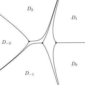
$t=t_{c}+{\rm i}\epsilon$

Figure 1. Stokes graphs for several $t$ (with $\nu=1$). Here we choose $t_{c}=-5$ and $\epsilon=1/2$.

The main conjectural ansatzs for the computation of Stokes multipliers around $x=\infty$ are the following:

• If the Stokes graph does not contain any saddle connection (i.e., a Stokes curve connecting zeros of $\varphi$), then the partition function (5) is Borel summable. Moreover, the discrete Fourier series

  $${\mathscr{T}}(t,\nu,\rho;g_{s})=\sum_{k\in{\mathbb{Z}}}{\rm e}^{2\pi{\rm i}k\rho/g_{s}}{\mathcal{Z}}(t,\nu+kg_{s};g_{s})$$ (18)

  converges and gives an analytic $\tau$-function of Painlevé I. Here, ${\mathcal{Z}}$ is the Borel sum of the partition function $Z$.

• Under the same saddle-free condition, the WKB-type series $\chi_{\pm}$ defined in (14) is Borel summable on each Stokes region. Moreover,

  $${\mathscr{Y}}_{\pm}(x,t,\nu,\rho;g_{s})=\frac{\displaystyle\sum_{k\in{\mathbb{Z}}}{\rm e}^{2\pi{\rm i}k\rho/g_{s}}\,{\mathcal{Z}}(t,\nu+kg_{s};g_{s})\,{\mathcal{X}}_{\pm}(x,t,\nu+kg_{s};g_{s})}{\displaystyle\sum_{k\in{\mathbb{Z}}}{\rm e}^{2\pi{\rm i}k\rho/g_{s}}\,{\mathcal{Z}}(t,\nu+kg_{s};g_{s})}$$ (19)

  converges and give an analytic solution of the isomonodromy system (LABEL:eq:Lax-PI) on the Stokes region. Here, ${\mathcal{X}}_{\pm}$ is the Borel sum of $\chi_{\pm}$.

• Under the same saddle-free condition, the Borel sums ${\mathcal{X}}_{\pm}$ of the WKB-type series (14) defined on adjacent faces of the Stokes graph are related by the Voros connection formula [Vor83, Sil85, KT05] (or the path-lifting rule in the sense of Gaiotto–Moore–Neitzke [GMN13b]).

The assumption (i) is consistent with the conjecture in [DMnP11, GMn22a, GKPKMn23] which claims the Borel singularities appear on the lattice generated by the integral periods of $y{\rm d}x$. Note that the saddle-free condition in (i) is satisfied if all the integral periods of $y{\rm d}x$ on the spectral curve have a non-zero imaginary part. Under the assumption (ii), we have five canonical solutions ${\mathscr{Y}}^{(j)}_{\pm}$ defined in the Stokes region $D_{j}$ in Figure 1 ($j=0,\pm 1,\pm 2$ mod $5$). Then, we define the Stokes multiplier $s_{j}$ attached to the $j$-th singular direction $\arg x=2\pi j/5$ as the non-trivial entry of the Stokes matrix ${\mathcal{S}}_{j}$ defined by

$$({\mathscr{Y}}^{(j+1)}_{+},{\mathscr{Y}}^{(j+1)}_{-})=({\mathscr{Y}}^{(j)}_{+},{\mathscr{Y}}^{(j)}_{-})\cdot{\mathcal{S}}_{j},$$ (20)

where

$${\mathcal{S}}_{j}=\begin{cases}\begin{pmatrix}1&s_{j}\\ 0&1\end{pmatrix}&j=0,\pm 2\\[20.00003pt] \begin{pmatrix}1&0\\ s_{j}&1\end{pmatrix}&j=\pm 1.\end{cases}$$ (21)

The assumption (iii) enables us to describe these Stokes multipliers explicitly via the Voros symbols ${\rm e}^{2\pi{\rm i}\nu/g_{s}}$ and ${\rm e}^{2\pi{\rm i}\rho/g_{s}}$. A rough explanation is the following: The Voros connection formula allows us to describe the analytic continuation of Borel resummed WKB solution by the term-wise analytic continuations on the spectral curve, and the formula (15) gives an explicit description of those analytic continuations in terms of the Voros symbols (see [Iwa20, §5] for details.). We will present the resulting Stokes multipliers in the next subsection.

2.3. Dillinger–Delabaere–Pham formula and non-linear Stokes phenomenon

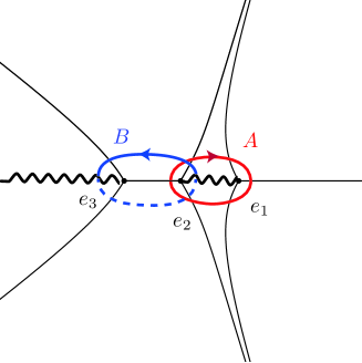
Figure 2. $A$-cycle and $B$-cycle.

Now, let us discuss the non-linear Stokes phenomenon in the Painlevé equation. We borrow the idea of Takei used in [Tak95, Tak00] where he relates the mutation of Stokes graph (which we will explain shortly) to non-linear Stokes phenomenon of Painlevé transcendents, through the invariance of the Stokes multipliers of (LABEL:eq:Lax-PI). This idea has been recently further developed in [BSSV23, vSV22]. We also note that our result is closely related to [Kap04, FIKN06] based on the Riemann–Hilbert method.

Figure 1 depicts Stokes graphs for $\nu=1$ and several $t$’s which are close to

$$t_{c}=-5.$$ (22)

Let us label the three zeros of $\varphi(x)$ at $t=t_{c}$ as

$$e_{1}\fallingdotseq 1.59075,\qquad e_{2}\fallingdotseq-0.01288,\qquad e_{3}\fallingdotseq-1.57157,$$ (23)

and take the $A$ cycle (resp., the $B$ cycle) as the cycle encircling the zeros $e_{1}$ and $e_{2}$ (resp., $e_{2}$ and $e_{3}$). Here the orientation of these cycle is given so that

$$\oint_{A}y{\rm d}x=2\int^{e_{1}}_{e_{2}}y{\rm d}x,\qquad\oint_{B}y{\rm d}x=-2\int^{e_{2}}_{e_{3}}y{\rm d}x,$$ (24)

where the branch of $y$ is chosen so that it has a positive imaginary part (resp., a negative real part) on the segment $[e_{2},e_{1}]$ (resp., $[e_{3},e_{2}]$). We may observe that a saddle connection appears at $t=t_{c}$, where the $B$-period

$$\oint_{B}y{\rm d}x\fallingdotseq 5.87065$$ (25)

of $y{\rm d}x$ has zero imaginary part. As we have mentioned in §2.2, we expect that this induces singularities on the positive real axis on the Borel-plane, and we will discuss the action of Stokes automorphism below.

The saddle connection is resolved and we have saddle-free Stokes graphs under a small variation of $t$ since the $B$-periods of $ydx$ are no longer real:

$$\oint_{B}y{\rm d}x\fallingdotseq\begin{cases}\displaystyle 5.83465+1.47447{\rm i}&\text{at $t=t_{c}-{\rm i}\epsilon$}\\ \displaystyle 5.83465-1.47447{\rm i}&\text{at $t=t_{c}+{\rm i}\epsilon$}.\end{cases}$$ (26)

Here we take $\epsilon=1/2$. We can observe that the topology of the Stokes graphs changes discontinuously before and after the appearance of the saddle connection. This is what we call the mutation of the Stokes graph.

Since the Stokes graphs at $t=t_{c}\pm{\rm i}\epsilon$ are saddle-free, we can use the recipe of [Iwa20, §5] to compute the Stokes multipliers around $x=\infty$. The resulting Stokes multipliers are

At $$t=t_{c}-{\rm i}\epsilon :\quad\begin{cases}s_{-2}={\rm i}\,{\rm e}^{2\pi{\rm i}\nu/g_{s}}\\ s_{-1}={\rm i}\,({\rm e}^{-2\pi{\rm i}\nu/g_{s}}-{\rm e}^{-2\pi{\rm i}(\nu+\rho)/g_{s}}+{\rm e}^{-2\pi{\rm i}\rho/g_{s}})\\ s_{0}\hskip 6.00006pt={\rm i}\,{\rm e}^{2\pi{\rm i}\rho/g_{s}}\\ s_{1}\hskip 6.00006pt={\rm i}\,{\rm e}^{-2\pi{\rm i}\rho/g_{s}}(1-{\rm e}^{2\pi{\rm i}\nu/g_{s}})\\ s_{2}\hskip 6.00006pt={\rm i}\,{\rm e}^{-2\pi{\rm i}\nu/g_{s}}(1-{\rm e}^{2\pi{\rm i}\rho/g_{s}}).\end{cases}$$ (27)

At $$t=t_{c}+{\rm i}\epsilon :\quad\begin{cases}{s}_{-2}={\rm i}\,{\rm e}^{2\pi{\rm i}\nu/g_{s}}(1-{\rm e}^{2\pi{\rm i}\rho/g_{s}})\\ {s}_{-1}={\rm i}\,{\rm e}^{-2\pi{\rm i}\rho/g_{s}}(1-{\rm e}^{-2\pi{\rm i}\nu/g_{s}})\\ {s}_{0}\hskip 6.00006pt={\rm i}\,{\rm e}^{2\pi{\rm i}\rho/g_{s}}\\ {s}_{1}\hskip 6.00006pt={\rm i}\,({\rm e}^{-2\pi{\rm i}\rho/g_{s}}-{\rm e}^{2\pi{\rm i}(\nu-\rho)/g_{s}}+{\rm e}^{2\pi{\rm i}\nu/g_{s}})\\ {s}_{2}\hskip 6.00006pt={\rm i}\,{\rm e}^{-2\pi{\rm i}\nu/g_{s}}.\end{cases}$$ (28)

We can check that the consistency conditions (c.f., [vdPS09])

$$1+s_{j-1}s_{j}+{\rm i}\,s_{j}+2=0\quad(s_{j}=s_{j+5})$$ (29)

of the Stokes multipliers are satisfied for both cases. We note that the result agrees with the computation of [BSSV23, §7.4]. This is also consistent with [Tak00, vSV22] through the identification of [BSSV23, (7.71)–(7.72)].

Thus, we have seen that the mutation of Stokes graphs induces a discontinuous change of the expressions of the Stokes multipliers. It is easy to observe that the Stokes data (28) are obtained from (27) by the transformation

$$({\rm e}^{2\pi{\rm i}\nu/g_{s}},{\rm e}^{2\pi{\rm i}\rho/g_{s}})\mapsto({\rm e}^{2\pi{\rm i}\nu/g_{s}}\,(1-{\rm e}^{2\pi i\rho/g_{s}}),{\rm e}^{2\pi{\rm i}\rho/g_{s}})$$ (30)

In fact, this is an example of a cluster transformation (or a Kontsevich–Soibelman transformation). Our observation is consistent with the results [DDP93, DP99, GMN13a, IN14, IN16] where the mutation of Stokes graphs induces a cluster transformation for the Voros symbols (the quantum period, the Fock-Goncharov coordinates). (30) is an example of the Delabaere–Dillinger–Pham (DDP) formula.

Now we get to the crucial point. Since $t$ is the isomonodromic time, these Stokes multipliers must be preserved under the variation of $t$. Therefore, the above formulas suggest the following: Let $(\nu^{+},\rho^{+})$ and $(\nu^{-},\rho^{-})$ be possibly different pairs of parameters, and let ${\mathscr{T}}^{\pm}(t,\nu^{\pm},\rho^{\pm},g_{s})$ be the Borel sum of $\tau(t,\nu^{\pm},\rho^{\pm},g_{s})$ defined at $t=t_{c}\pm{\rm i}\epsilon$. If these $\tau$-functions correspond to a common solution of Painlevé I, then they must be glued at $t=t_{c}$ so that the corresponding Stokes multipliers are identical. Namely, we have

$${\mathscr{T}}_{P_{\rm I}}^{-}(t,\nu^{-},\rho^{-};g_{s})={\rm e}^{\frac{1}{2\pi{\rm i}}{\rm Li}_{2}({\rm e}^{2\pi{\rm i}\rho^{+}/g_{s}})}{\mathscr{T}}_{P_{\rm I}}^{+}(t,\nu^{+},\rho^{+};g_{s})$$ (31)

with

$$(\nu^{+},\rho^{+})=\left(\nu^{-}-\frac{g_{s}}{2\pi{\rm i}}\log(1-{\rm e}^{2\pi{\rm i}\rho^{-}/g_{s}}),\rho^{-}\right).$$ (32)

Here, the prefactor $\exp(\frac{1}{2\pi{\rm i}}{\rm Li}_{2}(e^{2\pi{\rm i}\rho^{+}/g_{s}}))$ on the right hand side is related to the generating function of the monodromy symplectomorphism (which is the cluster transformation in this case); see [LR17, CLT20, BK21].

This formula can be regarded as the connection formula which describes the non-linear Stokes phenomenon for the Painlevé transcendents. We may write the formula in terms of the Stokes automorphism as

$${\mathfrak{S}}\tau(t,\nu,\rho;g_{s})={\rm e}^{\frac{1}{2\pi{\rm i}}{\rm Li}_{2}(e^{2\pi{\rm i}\rho/g_{s}})}\tau\left(t,\nu-\frac{g_{s}}{2\pi{\rm i}}\log(1-e^{2\pi{\rm i}\rho/g_{s}}),\rho;g_{s}\right).$$ (33)

If we look at the zero Fourier mode (i.e., coefficient of $e^{2\pi{\rm i}k\rho/g_{s}}$ with $k=0$), we have the all order instanton corrections of the partition function:

$${\mathfrak{S}}Z(t,\nu;g_{s})=\sum_{n=0}^{\infty}Z^{(n)}(t,\nu;g_{s})$$ (34)

with the terms of the form

$$Z^{(n)}(t,\nu;g_{s})=\mathfrak{Z}^{(n)}(t,\nu-ng_{s};g_{s})\,Z(t,\nu-ng_{s};g_{s}).$$ (35)

Here, $\mathfrak{Z}^{(n)}(t,\nu;g_{s})$ is a differential polynomial of the free energy $F(t,\nu;g_{s})$ with respect to $\nu$. The Seiberg–Witten relation $\partial_{\nu}F_{0}=\oint_{B}y{\rm d}x$ implies that $Z^{(n)}$ is a formal power series in $g_{s}$ with an exponential factor ${\rm e}^{-n\oint_{B}y{\rm d}x/g_{s}}$. Namely, $Z^{(n)}$ is an $n$-instanton amplitude. It turns out that the first few terms

$$Z^{(0)}(t,\nu;g_{s}) =Z(t,\nu;g_{s})$$ (36)

$$Z^{(1)}(t,\nu;g_{s}) =\left(1+\frac{g_{s}}{2\pi{\rm i}}\frac{\partial F}{\partial\nu}(t,\nu-g_{s};g_{s})\right)Z(t,\nu-g_{s};g_{s})$$ (37)

of (34) precisely agree (up to a normalization factor) with the multi-instanton results for the topological string obtained in [GMn22a, GKPKMn23]. In the next section, we will show that the agreement occurs for all $n$ as well. We may also observe that the first few terms of the 1-instanton part (37) are consistent with a known connection formula for Painlevé I (see e.g. [Kap88, Kap04]). This supports our heuristic derivation of (33).

Before ending the section, let us make a remark on a relation with the results of [Tak00, BSSV23, vSV22]. These works also derive a connection formula for solutions of Painlevé I through the isomonodromy property. Our result (33) describes the connection formula at the level of $\tau$-function, and the main difference is the appearance of the prefactor given by the dilogarithm function. The factor disappears in the solution of Painlevé I due to the logarithmic derivative (10). As we’ll see in the next section, we can relate the connection formula of Painlevé I with the results of [GMn22a, GKPKMn23] thanks to the prefactor. This is our new observation.

3. Resurgent structure and Stokes automorphisms in topological string theory

In this section we show that the main result from the previous section, (33), is a consequence of the conjectures of [GMn22a, GKPKMn23] on the resurgent structure of the topological string.

3.1. Resurgent structure of the topological string

In [GMn22a, GKPKMn23] a general conjecture on the resurgent structure of the topological string on arbitrary Calabi–Yau manifolds was put forward. This conjecture is based on a trans-series solution of the HAE of [BCOV94], as proposed in [CSESV16, CSESV15]. For this reason, it applies to the free energies obtained by doing topological recursion on curves of genus $g\geq 1$, but it also applies to the free energies of compact Calabi–Yau threefolds, since both are perturbative solutions to the HAE. For simplicity, we will first present the results in the one-modulus, local case originally studied in [GMn22a]. The generalization to the multi-modulus, general case is straightforward and will be presented below.

The conjecture of [GMn22a, GKPKMn23] is as follows. First, it asserts that Borel singularities of the topological string free energy are integral periods of the Calabi-Yau manifold, up to some overall normalization (in the local case, this was already conjectured in [DMnP11]). In the one-modulus, local case, this means that the singularity ${\mathcal{A}}$ can be written as

$${\mathcal{A}}=c\partial_{\nu}F_{0}+d\nu+d_{0},$$ (38)

where $c,d,d_{0}$ are integer numbers, times a normalization factor which depends on the normalization of $g_{s}$ (see [GKPKMn23] for a detailed discussion of normalizations). We will assume that ${\mathcal{A}}$ is a primitive vector of the period lattice. Then, $\ell{\mathcal{A}}$, with $\ell\in{\mathbb{Z}}_{>0}$ is also a Borel singularity, and we are interested in the structure of these “multi-instanton" singularities. There are two different situations. When $c=0$, the resurgent structure is of the Pasquetti–Schiappa form [PS10]. This means the following. Let us define

$$F^{(\ell)}_{\mathcal{A}}=\left({1\over\ell}{{\mathcal{A}}\over g_{s}}+{1\over\ell^{2}}\right){\rm e}^{-\ell{\mathcal{A}}/g_{s}}.$$ (39)

Then, the alien derivatives of the free energy are given by

$$\dot{\Delta}_{\ell{\mathcal{A}}}F=aF^{(\ell)}_{\mathcal{A}},\qquad\ell\in{\mathbb{Z}}_{>0},$$ (40)

where $a$ is a Stokes constant. When $c\not=0$, one defines a modified genus zero free energy $\tilde{F}_{0}$ by the equation

$${\mathcal{A}}=c\partial_{\nu}\tilde{F}_{0}.$$ (41)

We note that $\tilde{F}_{0}$ differs from the original $F_{0}$ in a quadratic polynomial in $\nu$. The total free energy appearing in the formulae for the trans-series involves $\tilde{F}_{0}$, i.e. it is given by

$$F(\nu;g_{s})=g_{s}^{-2}\tilde{F}_{0}(\nu)+\sum_{g\geq 1}g_{s}^{2g-2}F_{g}(\nu).$$ (42)

Let us now define

$$F^{(\ell)}=\left({\hbar F^{\prime}_{-\ell}\over\ell}+{1\over\ell^{2}}\right){\rm e}^{F_{-\ell}-F},$$ (43)

where we have introduced the rescaled coupling constant

$$\hbar=cg_{s}$$ (44)

and the notation

$$F_{k}(\nu;g_{s})=F(\nu+k\hbar;g_{s}).$$ (45)

The prime in (43) and other equations in this section denotes derivative w.r.t. $\nu$. Then, the alien derivatives of $F$ are given by

$$\dot{\Delta}_{\ell{\mathcal{A}}}F=aF^{(\ell)},\qquad\ell\in{\mathbb{Z}}_{>0}.$$ (46)

These are the main conjectures of [GMn22a, GKPKMn23]. They recover and extend partial results along this direction in [CSESV16, CSESV15, CSMnS17]. We note that both in (46) and (40) it is assumed that the Stokes constant is independent of $\ell$.

From the formulae for the alien derivatives one can compute the Stokes automorphism, through Écalle’s formula (see e.g. [MS16])

$$\mathfrak{S}_{\mathcal{C}}=\exp\left(\sum_{\ell=1}^{\infty}{\mathcal{C}}^{\ell}\dot{\Delta}_{\ell{\mathcal{A}}}\right).$$ (47)

We have introduced an additional formal parameter ${\mathcal{C}}$ to keep track of $\ell$. In view of the results of the previous section, we should consider the action of the Stokes automorphism on the partition function, $Z$, and we have

$$\mathfrak{S}_{{\mathcal{C}}}(Z)=\exp\left(\mathfrak{S}_{{\mathcal{C}}}(F)\right).$$ (48)

We have again two cases to consider. The simplest one is when $c=0$. In that case, the action of more than one alien derivative vanishes, and we simply have

$$\mathfrak{S}_{{\mathcal{C}}}(Z)=\exp\left(a\sum_{\ell=1}^{\infty}{\mathcal{C}}^{\ell}F^{(\ell)}_{\mathcal{A}}\right)Z=\exp\left(a\sum_{\ell=1}^{\infty}{\mathcal{C}}^{\ell}\left({1\over\ell}{{\mathcal{A}}\over g_{s}}+{1\over\ell^{2}}\right){\rm e}^{-\ell{\mathcal{A}}/g_{s}}\right)Z,$$ (49)

which we can write as

$$\mathfrak{S}_{{\mathcal{C}}}(Z)=\exp\left(a\,{\rm Li}_{2}({\mathcal{C}}\,{\rm e}^{-{\mathcal{A}}/g_{s}})-a{{\mathcal{A}}\over g_{s}}\log(1-{\mathcal{C}}\,{\rm e}^{-{\mathcal{A}}/g_{s}})\right)Z.$$ (50)

This is the result obtained for the resolved conifold after using the Pasquetti–Schiappa form (see e.g. [ASTT23]). We note that the ingredients for our main formula (the dilogarithm and the logarithm) are already here, and they follow from the Pasquetti–Schiappa form of the multi-instanton amplitudes, which is in turn ultimately due to the universal behavior of the topological string at the conifold point [GV95].

The non-trivial case for the calculation of the Stokes automorphism occurs when $c\not=0$, since one has to act with multiple alien derivatives. Explicit calculations show that the result has the form

$$\mathfrak{S}_{{\mathcal{C}}}(Z)=\sum_{\ell\geq 0}{\mathcal{C}}^{\ell}\mathfrak{Z}^{(\ell)}(\nu-\ell\hbar)Z(\nu-\ell\hbar;g_{s}),$$ (51)

where $\mathfrak{Z}^{(\ell)}(\nu)$ can be computed explicitly and $\mathfrak{Z}^{(0)}=1$. One finds, for the very first values,

$$\mathfrak{Z}^{(1)} =a\left(1+\hbar F^{\prime}\right),$$ (52)

$$\mathfrak{Z}^{(2)} ={a^{2}\over 2}\left(1+2\hbar F^{\prime}+(\hbar F^{\prime})^{2}+\hbar^{2}F^{\prime\prime}\right)+a\left({1\over 4}+{\hbar F^{\prime}\over 2}\right).$$

This is in accord with (34), (35). We will show in the next subsection that the structure (51) follows from the results of [GMn22a]. The arguments in section 2 suggest in addition the following explicit generating functional for the functions $\mathfrak{Z}^{(\ell)}(\nu)$:

$$Z(\nu;g_{s})\sum_{\ell\geq 0}{\mathcal{C}}^{\ell}\mathfrak{Z}^{(\ell)}(\nu)={\rm e}^{a{\rm Li}_{2}({\mathcal{C}})}Z\left(\nu-\hbar a\log(1-{\mathcal{C}});g_{s}\right).$$ (53)

Indeed, it follows from (51) and (53) that

$$\mathfrak{S}_{{\mathcal{C}}}(Z)=\exp\left\{a{\rm Li}_{2}\left({\mathcal{C}}{\rm e}^{-\hbar\partial}\right)-\hbar a\log\left(1-{\mathcal{C}}{\rm e}^{-\hbar\partial}\right)\partial\right\}Z,$$ (54)

where $\partial$ is the derivative w.r.t. $\nu$. If we introduce now the discrete Fourier transform as in (8),

$$\tau(\nu,\rho;g_{s})=\sum_{k\in{\mathbb{Z}}}{\rm e}^{2\pi{\rm i}k\rho/g_{s}}Z(\nu+kg_{s};g_{s}),$$ (55)

one easily finds

$$\mathfrak{S}_{{\mathcal{C}}}\tau(\nu,\rho;g_{s})={\rm e}^{a{\rm Li}_{2}({\mathcal{C}}{\rm e}^{2\pi{\rm i}c\rho/g_{s}})}\tau\left(\nu-\hbar a\log(1-{\mathcal{C}}{\rm e}^{2\pi{\rm i}c\rho/g_{s}}),\rho;g_{s}\right),$$ (56)

where we have made a choice of normalizations in such a way that the coefficient $c$ is an integer. The formula above has precisely the structure anticipated in (33) (the two formulae agree after setting ${\mathcal{C}}=c=1$, $a=1/(2\pi{\rm i})$.) In subsection 3.3 we will consider a more general cases for the transformation of the dual partition function and make contact with the results of [AP16].

3.2. A derivation of the formula for Stokes automorphisms

We will now show that the formulae (53) and (54) follow from the conjecture on the alien derivatives of the free energy, (46). To do this, we will rely on various results of [GMn22a, GKPKMn23], which we summarize very briefly here. We refer to those papers for more details.

In the framework of the HAE, the perturbative free energies $F_{g}$ are non-holomorphic but global functions on the moduli space. More precisely, they are polynomials in a non-holomorphic propagator $S$, whose coefficients are functions of a complex coordinate $z$ on the moduli space (not necessarily flat). The conventional free energies are holomorphic but can be defined in different frames, which are determined by a choice of $A$ and $B$ periods. The holomorphic free energies in different frames are obtained by considering the non-holomorphic free energies, and taking different holomorphic limits of the propagator. We define the ${\mathcal{A}}$-frame as the frame in which ${\mathcal{A}}$ is the $A$-period, and the holomorphic propagator appropriate for the ${\mathcal{A}}$-frame will be denoted by $S_{\mathcal{A}}$. The boundary conditions to solve the HAE are obtained by evaluating the holomorphic free energies in different frames and imposing particular behaviors at special points in moduli space, in particular the universal behaviour at the conifold point [GV95] and the resulting gap condition [HK07].

It was pointed out in [CSESV16, CSESV15, CSMnS17] that the resurgent structure of the topological string free energy can be obtained by considering trans-series solutions to the HAE of [BCOV94]. The solutions corresponding to the $\ell$-th instanton sector are formal power series in $g_{s}$, whose coefficients are also polynomials in $S$ with $z$-dependent coefficients, and they also involve ${\mathcal{A}}$ and their derivatives (the second derivative of ${\mathcal{A}}$ can be however re-expressed in terms of $S_{\mathcal{A}}$). The $\ell$-instanton amplitude involves of course an exponential prefactor of the form ${\rm e}^{-\ell{\mathcal{A}}/g_{s}}$. Explicit trans-series solutions were obtained in [GMn22a, GKPKMn23] by using an operator formalism first suggested in [CMnS19, Cod18]. The main operator in this formalism is

$$\mathsf{D}=g_{s}\partial_{z}{\mathcal{A}}(S-S_{\mathcal{A}})\partial_{z}.$$ (57)

When evaluated in the holomorphic limit, this operator becomes $\hbar\partial_{\nu}$, i.e. a derivative w.r.t. the flat coordinate $\nu$.

We are now ready to prove the formula (53). The Stokes automorphism, acting on $Z$, is a formal sum of multi-instanton sectors which has to solve the HAE for the partition function, and in addition it has to satisfy the following boundary condition: when evaluated at the ${\mathcal{A}}$-frame, it is equal to (50). This determines its form uniquely. A general $n$-th instanton solution to the HAE for the partition function was determined in [GMn22a] and has the structure:

$$Z^{(n)}=\mathfrak{A}_{n}\,{\rm e}^{-\Phi_{n}}Z,$$ (58)

where

$$\Phi_{n}={1\over\mathsf{D}}\left(1-{\rm e}^{-n\mathsf{D}}\right)G,\qquad G={1\over g_{s}}{\mathcal{A}}+\mathsf{D}(F-g_{s}^{-2}F_{0}).$$ (59)

Let us note that, in the holomorphic limit,

$$\Phi_{n}\rightarrow F(\nu;g_{s})-F(\nu-n\hbar;g_{s}).$$ (60)

The prefactor $\mathfrak{A}_{n}$ is determined as follows. Let

$$X_{n}={\rm e}^{-n\mathsf{D}}G.$$ (61)

Then, the $\mathfrak{A}_{n}$ are arbitrary linear combinations of the objects $\mathfrak{w}_{\ell}$, defined by

$$\mathfrak{w}_{\ell}=\sum_{\boldsymbol{k},\,d(\boldsymbol{k})=\ell}C_{\boldsymbol{k}}\mathfrak{X}_{\boldsymbol{k}}.$$ (62)

In this formula, $\boldsymbol{k}=(k_{1},k_{2},\cdots)$ is a vector of non-negative entries, $d(\boldsymbol{k})$ is given by

$$d(\boldsymbol{k})=\sum_{j}jk_{j},$$ (63)

the coefficients $C_{\boldsymbol{k}}$ are of the form,

$$C_{\boldsymbol{k}}={\ell!\over\prod_{j\geq 1}k_{j}!(j!)^{k_{j}}},$$ (64)

and

$$\mathfrak{X}_{\boldsymbol{k}}=X_{n}^{k_{1}}(\mathsf{D}X_{n})^{k_{2}}(\mathsf{D}^{2}X_{n})^{k_{3}}\cdots.$$ (65)

We would like to emphasize that this structure is determined by requiring that (58) is a solution to the HAE. Let us also note that all the $X$’s appearing in $\mathfrak{A}_{n}$ are shifted, i.e. they are acted by the automorphism ${\rm e}^{-n\mathsf{D}}$, so it is convenient to introduce the “unshifted" prefactor $\mathfrak{B}_{n}$ defined by

$$\mathfrak{A}_{n}={\rm e}^{-n\mathsf{D}}\mathfrak{B}_{n}.$$ (66)

In $\mathfrak{B}_{n}$, $X_{n}$ is replaced by $X=G$. The precise linear combination of $\mathfrak{w}_{\ell}$ appearing in $\mathfrak{A}_{n}$ is uniquely determined by the boundary condition, i.e. by its form in the ${\mathcal{A}}$-frame. Let us suppose that, when evaluated in the ${\mathcal{A}}$-frame, the holomorphic limit of $Z^{(n)}$ is of the form

$$Z^{(n)}_{\mathcal{A}}=\left\{\sum_{k}c_{n,k}\left({{\mathcal{A}}\over g_{s}}\right)^{k}\right\}{\rm e}^{-n{\mathcal{A}}/g_{s}}Z_{\mathcal{A}},$$ (67)

where the prefactor is an arbitrary polynomial in ${\mathcal{A}}/g_{s}$. Then,

$$\mathfrak{B}_{n}=\sum_{k}c_{n,k}\mathfrak{w}_{k}.$$ (68)

Let us now apply these results to the calculation of the Stokes automorphism. As we explained before, the Stokes automorphism is the holomorphic limit of a formal linear combination of solutions of the form (58). Therefore, we must have

$$\mathfrak{S}_{{\mathcal{C}}}(Z)=\sum_{\ell\geq 0}{\mathcal{C}}^{\ell}\mathfrak{A}_{\ell}Z(\nu-\hbar\ell;g_{s}).$$ (69)

(To lighten the notation, we are using the same symbols for the non-holomorphic quantities appearing in the HAE, and for their holomorphic limits. Hopefully, which one is being used at a given moment is clear from the context.) This is precisely the structure of (51), which follows from the general results for multi-instantons. We deduce that

$$\mathfrak{A}_{\ell}=\mathfrak{Z}^{(\ell)}(\nu-\hbar\ell).$$ (70)

Both sides involve functions whose argument is shifted by $-\hbar\ell$. In terms of the unshifted prefactors introduced in (66) we have

$$\mathfrak{B}_{\ell}=\mathfrak{Z}^{(\ell)}(\nu).$$ (71)

The boundary condition obtained from (50) is

$$\sum_{n\geq 0}{\mathcal{C}}^{n}\mathfrak{B}_{n,{\mathcal{A}}}=\exp\left(a{\rm Li}_{2}({\mathcal{C}})-a{{\mathcal{A}}\over g_{s}}\log(1-{\mathcal{C}})\right)={\rm e}^{a{\rm Li}_{2}({\mathcal{C}})}\sum_{k\geq 0}{1\over k!}\left(-a\log(1-{\mathcal{C}})\right)^{k}\left({{\mathcal{A}}\over g_{s}}\right)^{k}.$$ (72)

According to what we explained before, we can already write the general solution to the HAE, by simply replacing $({\mathcal{A}}/g_{s})^{k}$ by $\mathfrak{w}_{k}$:

$$\sum_{n\geq 0}{\mathcal{C}}^{n}\mathfrak{Z}^{(n)}={\rm e}^{a{\rm Li}_{2}({\mathcal{C}})}\sum_{k\geq 0}{1\over k!}\left(-a\log(1-{\mathcal{C}})\right)^{k}\mathfrak{w}_{k},$$ (73)

where we have already used (71). It was proven in [GMn22a] that

$$\Xi(\xi)=\sum_{\ell\geq 0}{\xi^{\ell}\over\ell!}\mathfrak{w}_{\ell}=\exp\left(\sum_{j=1}^{\infty}{\xi^{j}\over j!}\mathsf{D}^{j-1}X\right),$$ (74)

where $\xi$ is an arbitrary complex parameter. We conclude that

$$\sum_{n\geq 0}{\mathcal{C}}^{n}\mathfrak{Z}^{(n)}={\rm e}^{a{\rm Li}_{2}({\mathcal{C}})}\exp\left({1\over\mathsf{D}}\left({\rm e}^{-a\log(1-{\mathcal{C}})\mathsf{D}}-1\right)X\right),$$ (75)

In the holomorphic limit, we have that

$$X\rightarrow\hbar\partial_{\nu}F$$ (76)

where $F$ is the total free energy, and we get in the end

$$\sum_{n\geq 0}{\mathcal{C}}^{n}\mathfrak{Z}^{(n)}=\exp\left(a{\rm Li}_{2}({\mathcal{C}})+F(\nu-a\hbar\log(1-{\mathcal{C}});g_{s})-F(\nu;g_{s})\right).$$ (77)

This is precisely (53).

3.3. Generalizations

The above results concern the one-modulus, local case. However, the generalization to arbitrary CY threefolds is straightforward, by using the results of [GKPKMn23] (to which we refer for further details). We will now write in some detail the more general formula for the Stokes automorphism. In the case of an arbitrary CY, the genus $g$ free energies depend on the “big moduli space" flat coordinates $X^{I}$ of the CY, where $I=0,1,\cdots,n$. The Borel singularities or instanton actions are again integral periods, given by linear combinations,

$$\kappa^{-1}{\mathcal{A}}=c^{I}{\partial F_{0}\over\partial X^{I}}+d_{I}X^{I}.$$ (78)

Here, we have introduced explicitly the normalization factor $\kappa$ relating the action to the integral periods. If all $c^{I}=0$, the multi-instanton amplitudes are again of the Pasquetti–Schiappa form (39) and the Stokes automorphism is given by (50). When not all $c^{I}$ vanish, one defines a new genus zero free energy by

$${\mathcal{A}}=\kappa c^{I}{\partial\tilde{F}_{0}\over\partial X^{I}},$$ (79)

as in the local case. It can be written as

$$\tilde{F}_{0}(X^{I})=F_{0}(X^{I})+{1\over 2}a_{IJ}X^{I}X^{J},\qquad a_{IJ}c^{I}=d_{J}.$$ (80)

Of course, the final formulae will not depend on $a_{IJ}$, but only on $c^{I}$, $d_{J}$. As shown in [GKPKMn23], one has to define a new genus one free energy

$$\tilde{F}_{1}=F_{1}-\left({\chi\over 24}-1\right)\log X^{0}.$$ (81)

Such a redefinition has appeared before in e.g. eq. (2.77) of [APP11]. The total free energy relevant for the multi-instanton amplitudes will be denoted by $\tilde{F}(X^{I};g_{s})$, and is given by

$$\widetilde{F}(X^{I};g_{s}) =g_{s}^{-2}\tilde{F}_{0}(X^{I})+\tilde{F}_{1}(X^{I})+\sum_{g\geq 2}g_{s}^{2g-2}F_{g}(X^{I})$$ (82)

$$={1\over 2g_{s}^{2}}a_{IJ}X^{I}X^{J}+F(X^{I};g_{s}).$$

Then, one has the following generalization of (54),

$$\mathfrak{S}_{{\mathcal{C}}}(\tilde{Z})=\exp\left\{a{\rm Li}_{2}\left({\mathcal{C}}{\rm e}^{-\kappa g_{s}c^{I}\partial_{I}}\right)-a\kappa g_{s}\log\left(1-{\mathcal{C}}{\rm e}^{-\kappa g_{s}c^{I}\partial_{I}}\right)c^{I}\partial_{I}\right\}\tilde{Z},$$ (83)

where we have denoted $\tilde{Z}={\rm e}^{\tilde{F}}$, and

$$\partial_{I}={\partial\over\partial X^{I}}.$$ (84)

As we have explained before, the action of the Stokes automorphism has a simpler form when it acts on an appropriate dual partition function. We could obtain a direct generalization of (56) involving the redefined partition function $\tilde{Z}$. However, in order to make contact with the results of [AP16], it is convenient to consider the dual partition function to the original $Z$. This means that in (83) we have to treat separately the quadratic term in $X^{I}$ appearing in the second line of (82). If we denote

$$Y^{I}=X^{I}-a\kappa g_{s}c^{I}\log(1-{\mathcal{C}})$$ (85)

we find

$$\tilde{Z}\left(Y^{I};g_{s}\right)$$ (86)

$$=\exp\left\{{\kappa^{2}\over 2}a^{2}d^{I}c_{I}\log^{2}(1-{\mathcal{C}})-g_{s}^{-1}a\kappa\log(1-{\mathcal{C}})d_{I}X^{I}+{1\over 2g_{s}^{2}}a_{IJ}X^{I}X^{J}\right\}Z\left(Y^{I};g_{s}\right).$$

We also note that, for $n\in{\mathbb{Z}}$,

$${\rm e}^{-n\kappa g_{s}c^{I}\partial_{I}}\exp\left\{{1\over 2g_{s}^{2}}a_{IJ}X^{I}X^{J}\right\}=\exp\left\{-g_{s}^{-1}\kappa d_{I}X^{I}n+{n^{2}\over 2}\kappa^{2}c^{I}d_{I}\right\}\exp\left\{{1\over 2g_{s}^{2}}a_{IJ}X^{I}X^{J}\right\}.$$ (87)

We have to be more concrete about the normalization factor $\kappa$. It was found in [GKPKMn23] that, with the canonical normalization of $g_{s}$, one has

$$\kappa^{2}=-2\pi{\rm i},$$ (88)

and this means that

$${\rm e}^{{n^{2}\over 2}\kappa^{2}c^{I}d_{I}}={\rm e}^{-\pi{\rm i}nc^{I}d_{I}},$$ (89)

since $n,d_{I},c^{I}\in{\mathbb{Z}}$. We will now put together $c^{I}$, $d_{I}$ in a symplectic vector $\gamma=(c^{I},d_{I})$. Let us introduce

$$\boldsymbol{X}_{\gamma}=\sigma(\gamma)\exp\left[-\kappa g_{s}^{-1}\left(d_{I}X^{I}-\rho_{I}c^{I}\right)\right],$$ (90)

where $\rho_{I}$, $I=0,1,\cdots,n$, are additional variables, and

$$\sigma(\gamma)=(-1)^{d_{I}c^{I}}.$$ (91)

Then, one finds that (83) is equivalent to

$$\mathfrak{S}_{{\mathcal{C}}}\left(\sum_{\boldsymbol{\ell}\in{\mathbb{Z}}^{n}}{\rm e}^{\kappa\rho_{I}\ell^{I}/g_{s}}Z\left(X^{I}+\kappa\ell^{I}g_{s};g_{s}\right)\right)={\rm e}^{a{\rm Li}_{2}({\mathcal{C}}\boldsymbol{X}_{\gamma})-\pi{\rm i}a^{2}d^{I}c_{I}\log^{2}(1-{\mathcal{C}}\boldsymbol{X}_{\gamma})}$$ (92)

$$\times\sum_{\boldsymbol{\ell}\in{\mathbb{Z}}^{n}}{\rm e}^{-ag_{s}^{-1}\kappa\log(1-{\mathcal{C}}\boldsymbol{X}_{\gamma})d_{I}(X^{I}+\kappa g_{s}\ell^{I})}Z\left(X^{I}+\kappa g_{s}\ell^{I}-ag_{s}\kappa c^{I}\log\left(1-{\mathcal{C}}\boldsymbol{X}_{\gamma}\right);g_{s}\right){\rm e}^{\kappa\rho_{I}\ell^{I}/g_{s}}.$$

The appropriate definition of the dual partition function in this general case is [AP16]:

$$\tau(X^{I},\rho_{I};g_{s})={\rm e}^{{1\over 2g_{s}^{2}}X^{I}\rho_{I}}\sum_{\boldsymbol{\ell}\in{\mathbb{Z}}^{n}}Z\left(X^{I}+\kappa\ell^{I}g_{s};g_{s}\right){\rm e}^{\kappa\rho_{I}\ell^{I}/g_{s}},$$ (93)

and the action of the Stokes automorphism is

$$\mathfrak{S}\tau(X^{I},\rho_{I};g_{s})$$ (94)

$$=\exp\left(aL_{\sigma(\gamma)}(\boldsymbol{X}_{\gamma})\right)\tau\left(X^{I}-ag_{s}\kappa c^{I}\log\left(1-\boldsymbol{X}_{\gamma}\right),\rho_{I}-ag_{s}\kappa d_{I}\log\left(1-\boldsymbol{X}_{\gamma}\right);g_{s}\right),$$

where we have put ${\mathcal{C}}=1$, and $L_{\epsilon}(z)$ is the twisted Rogers dilogarithm, as in [AP16]:

$$L_{\epsilon}(z)={\rm Li}_{2}(z)+{1\over 2}\log(\epsilon^{-1}z)\log(1-z).$$ (95)

It is easy to see that (94) agrees precisely with the wall-crossing formula (1.9) in [AP16], where their variables $\xi^{I}$, $\tilde{\xi}_{I}$ are related to ours by $(X^{I},\rho_{I})=-\kappa g_{s}(\xi^{I},\tilde{\xi}_{I})$. In addition, the agreement between the formulae requires the identification (4). One advantage of (94) is that, when $c^{I}=0$, one recovers as well the transformation formula (50) (this is easily seen by looking e.g. at the mode with $\ell^{I}=0$).

There is another generalization of the formula (53) that one could consider. So far we have only included forward alien derivatives, and correspondingly purely instanton sectors. We can also consider alien derivatives in both the negative and the positive directions, which lead to amplitudes with both instantons and “negative instantons." Let us define

$$F^{(0|\ell)}(\nu;g_{s})=-F^{(\ell)}(\nu;-g_{s}),\qquad F^{(0|\ell)}_{\mathcal{A}}(\nu;g_{s})=-F^{(\ell)}_{\mathcal{A}}(\nu;-g_{s}).$$ (96)

The basic alien derivative in the negative direction is simply,

$$\dot{\Delta}_{-\ell{\mathcal{A}}}F=aF^{(0|\ell)}\qquad\text{or}\qquad aF^{(0|\ell)}_{\mathcal{A}},$$ (97)

depending on whether $c\not=0$ or $c=0$. We can then consider the “mixed" Stokes automorphism:

$$\mathfrak{S}_{{\mathcal{C}}_{1},{\mathcal{C}}_{2}}=\exp\left(\sum_{\ell\geq 1}{\mathcal{C}}_{1}^{\ell}\dot{\Delta}_{\ell{\mathcal{A}}}+{\mathcal{C}}_{2}^{\ell}\dot{\Delta}_{-\ell{\mathcal{A}}}\right).$$ (98)

Acting on $Z$, it has the structure

$$\mathfrak{S}_{{\mathcal{C}}_{1},{\mathcal{C}}_{2}}(Z)=\sum_{\ell_{1},\ell_{2}\geq 0}{\mathcal{C}}_{1}^{\ell_{1}}{\mathcal{C}}_{2}^{\ell_{2}}\mathfrak{Z}^{(\ell_{1}|\ell_{2})}(\nu-(\ell_{1}-\ell_{2})\hbar)Z\left(\nu-(\ell_{1}-\ell_{2})\hbar\right),$$ (99)

where $\mathfrak{Z}^{(0|0)}=1$. In this case, the boundary condition follows from (97), (96) and (39). It is given by,

$$\exp\left\{a\sum_{\ell=1}^{\infty}\left({\mathcal{C}}_{1}^{\ell}F^{(\ell)}_{\mathcal{A}}+{\mathcal{C}}_{2}^{\ell}F^{(0|\ell)}_{\mathcal{A}}\right)\right\}$$ (100)

$$=\exp\left\{a\left({\rm Li}_{2}({\mathcal{C}}_{1})-{\rm Li}_{2}({\mathcal{C}}_{2})\right)-a{{\mathcal{A}}\over g_{s}}\left(\log(1-{\mathcal{C}}_{1})+\log(1-{\mathcal{C}}_{2})\right)\right\}.$$

By using the results in [GMn22a], we can generalize (53) to

$$Z(\nu;g_{s}) \sum_{\ell_{1},\ell_{2}\geq 0}{\mathcal{C}}_{1}^{\ell_{1}}{\mathcal{C}}_{2}^{\ell_{2}}\mathfrak{Z}^{(\ell_{1}|\ell_{2})}(\nu)$$ (101)

$$={\rm e}^{a\left({\rm Li}_{2}({\mathcal{C}}_{1})-{\rm Li}_{2}({\mathcal{C}}_{2})\right)}Z\left(\nu-a\hbar\log(1-{\mathcal{C}}_{1})-a\hbar\log(1-{\mathcal{C}}_{2});g_{s}\right).$$

It is easy to write this formula in the form (83) or (94).

Appendix A Definition of correlators and free energy in topological recursion

To apply the topological recursion, we regard (6) as a family of spectral curves in the sense of [EO07] (i.e., a data consisting of a compact Riemann surface $C$ and a pair $(x,y)$ of meromorphic functions on it), through the Weierstrass parametrization:

$$C={\mathbb{C}}/\Lambda,\quad x(z)=\wp(z),\quad y(z)=\wp^{\prime}(z).$$ (102)

Here $\wp(z)=\wp(z;g_{2},g_{3})$ is the Weierstrass $\wp$-function with $g_{2}=-2t$ and $g_{3}=-u$, which is doubly-periodic with periods $\omega_{A}$ and $\omega_{B}$ (we omit the $t$ and $\nu$ dependence for simplicity). $\Lambda={\mathbb{Z}}\omega_{A}+{\mathbb{Z}}\omega_{B}$ is the lattice generated by the periods of the elliptic curve (6).

Let $z_{o}\in{\mathbb{C}}$ be a generic point, and $\Omega$ be the quadrilateral with $z_{o}$, $z_{o}+\omega_{A}$, $z_{o}+\omega_{B}$ and $z_{o}+\omega_{A}+\omega_{B}$ on its vertices; that is, a fundamental domain of ${\mathbb{C}}/\Lambda$. The ramification points (i.e., zeros of ${\rm d}x$) on $\Omega$ are given by the half-periods $r_{1}\equiv\omega_{A}/2$, $r_{2}\equiv\omega_{B}/2$ and $r_{3}\equiv(\omega_{A}+\omega_{B})/2$ modulo $\Lambda$. These points correspond to the branch points $e_{i}=x(r_{i})$ ($i=1,2,3$) of the elliptic curve which are defined by $4x^{3}+2tx+u=4(x-e_{1})(x-e_{2})(x-e_{3})$. The covering involution $y\mapsto-y$ is realized by $z\mapsto\sigma(z)\equiv-z$ mod $\Lambda$.

To run the topological recursion, we also need the Bergman bidifferential normalized along the chosen A-cycle, For our spectral curve, it is given by

$$B(z_{1},z_{2})=\Bigl{(}\wp(z_{1}-z_{2})+\frac{\eta_{A}}{\omega_{A}}\Bigr{)}\,{\rm d}z_{1}{\rm d}z_{2}.$$ (103)

Then, the Eynard–Orantin’s topological recursion recursively constructs a doubly-indexed sequence of meromorphic multi-differentials $\omega_{g,n}(z_{1},\dots,z_{n})$ ($g\geq 0$, $n\geq 1$) on the spectral curve, called correlators, as follows:

$$\omega_{0,1}(z_{1})=y(z_{1})\,{\rm d}x(z_{1}),\quad\omega_{0,2}(z_{1},z_{2})=B(z_{1},z_{2}),$$ (104)

and for $2g-2+n\geq 1$, we define

$$\omega_{g,n}(z_{1},\dots,z_{n})=\sum_{j=1}^{3}\mathop{\rm Res}_{z=r_{j}}\,K(z_{1},z)R_{g,n}(z,z_{2},\dots,z_{n}),$$ (105)

where

$$R_{g,n}(z,z_{2},\dots,z_{n})=\omega_{g-1,n+1}(z,\sigma(z),z_{2},\dots,z_{n})+\sum^{\prime}_{\begin{subarray}{c}g_{1}+g_{2}=g\\ I\sqcup J=\{2,\dots,n\}\end{subarray}}\omega_{g_{1},|I|+1}(z,z_{I})\,\omega_{g_{2},|J|+1}(\sigma(z),z_{J}).$$ (106)

Here, the recursion kernel $K(z_{1},z)$ is given by

$$K(z_{1},z)=\frac{1}{(y(z)-y(\sigma(z)))\,{\rm d}x(z)}\,\int^{w=z}_{w=0}\omega_{0,2}(z_{1},w).$$ (107)

We use the convention for tuple of variables as $z_{I}=(z_{i_{1}},\dots,z_{i_{k}})$ if $I=\{i_{1},\dots,i_{k}\}$, and the prime in the r.h.s. of (106) means that only indices satisfying $(g_{i},I_{i})\neq(0,\emptyset)$ are taken (i.e., $\omega_{0,1}$ does not appear) in the summation.

Here we also recall the definition of the genus $g$ free energy $F_{g}=F_{g}(t,\nu)$ introduced in [EO07]. The genus $0$ free energy $F_{0}$ is defined in [EO07, §4.2.2]. In our case, it is given by

$$F_{0}=\frac{t\,u}{5}+\frac{\nu}{2}\,\oint_{B}y{\rm d}x.$$ (108)

The genus $1$ free energy $F_{1}$ is also defined in [EO07, §4.2.3] up to a multiplicative constant. We employ

$$F_{1}=-\frac{1}{12}\log\Bigl{(}\omega_{A}^{6}\,{\mathcal{D}}\Bigr{)}$$ (109)

as the definition. Here

$${\mathcal{D}}=-8t^{3}-27u(t,\nu)^{2}\quad(=16(e_{1}-e_{2})^{2}(e_{2}-e_{3})^{2}(e_{3}-e_{1})^{2})$$ (110)

is the discriminant of (6). Finally, we define the genus $g$ free energy $F_{g}$ for $g\geq 2$ by

$$F_{g}=\frac{1}{2-2g}\,\sum_{j=1}^{3}\mathop{\rm Res}_{z=r_{j}}\,\Phi(z)\,\omega_{g,1}(z),$$ (111)

where $\Phi$ is any primitive of $\omega_{0,1}$. See [EO07] for properties of $\omega_{g,n}$ and $F_{g}$.

References

- [AP16] Sergei Alexandrov and Boris Pioline, Theta series, wall-crossing and quantum dilogarithm identities, Lett. Math. Phys. 106 (2016), no. 8, 1037–1066, 1511.02892.
- [APP11] Sergei Alexandrov, Daniel Persson, and Boris Pioline, Fivebrane instantons, topological wave functions and hypermultiplet moduli spaces, JHEP 03 (2011), 111, 1010.5792.
- [ASTT23] Murad Alim, Arpan Saha, Joerg Teschner, and Iván Tulli, Mathematical Structures of Non-perturbative Topological String Theory: From GW to DT Invariants, Commun. Math. Phys. 399 (2023), no. 2, 1039–1101, 2109.06878.
- [BCOV94] Michael Bershadsky, Sergio Cecotti, Hirosi Ooguri, and Cumrun Vafa, Kodaira–Spencer theory of gravity and exact results for quantum string amplitudes, Commun. Math. Phys. 165 (1994), 311–428, hep-th/9309140.
- [BE16] Vincent Bouchard and Bertrand Eynard, Reconstructing WKB from topological recursion, 1606.04498.
- [BK21] Marco Bertola and Dmitry Korotkin, Tau-Functions and Monodromy Symplectomorphisms, Commun. Math. Phys. 388 (2021), no. 1, 245–290, 1910.03370.
- [BKMnP09] Vincent Bouchard, Albrecht Klemm, Marcos Mariño, and Sara Pasquetti, Remodeling the B-model, Commun.Math.Phys. 287 (2009), 117–178, 0709.1453.
- [BLM+17] Giulio Bonelli, Oleg Lisovyy, Kazunobu Maruyoshi, Antonio Sciarappa, and Alessandro Tanzini, On Painlevé/gauge theory correspondence, Letters in Mathematical Physics 107 (2017), no. 12, 2359–2413.
- [BM23] Tom Bridgeland and Davide Masoero, On the monodromy of the deformed cubic oscillator, Mathematische Annalen 385 (2023), no. 1, 193–258.
- [Bri19] Tom Bridgeland, Riemann–Hilbert problems from Donaldson–Thomas theory, Inventiones mathematicae 216 (2019), no. 1, 69–124.
- [Bri23] by same author, Tau functions from Joyce structures, 2303.07061.
- [BS15] Tom Bridgeland and Ivan Smith, Quadratic differentials as stability conditions, Publ. Math. Inst. Hautes Études Sci. 121 (2015), 155–278.
- [BSSV23] Salvatore Baldino, Ricardo Schiappa, Maximilian Schwick, and Roberto Vega, Resurgent Stokes data for Painlevé equations and two-dimensional quantum (super) gravity, Commun. Num. Theor. Phys. 17 (2023), no. 2, 385–552, 2203.13726.
- [CLT20] Ioana Coman, Pietro Longhi, and Jörg Teschner, From quantum curves to topological string partition functions II, 2004.04585.
- [CMnS19] Santiago Codesido, Marcos Mariño, and Ricardo Schiappa, Non-Perturbative Quantum Mechanics from Non-Perturbative Strings, Annales Henri Poincare 20 (2019), no. 2, 543–603, 1712.02603.
- [Cod18] Santiago Codesido, A geometric approach to non-perturbative quantum mechanics, Ph.D. thesis, University of Geneva, 2018.
- [CSESV15] Ricardo Couso-Santamaría, Jose D. Edelstein, Ricardo Schiappa, and Marcel Vonk, Resurgent transseries and the holomorphic anomaly: Nonperturbative closed strings in local , Commun. Math. Phys. 338 (2015), no. 1, 285–346, 1407.4821.
- [CSESV16] Ricardo Couso-Santamaría, José D. Edelstein, Ricardo Schiappa, and Marcel Vonk, Resurgent transseries and the holomorphic anomaly, Annales Henri Poincaré 17 (2016), no. 2, 331–399, 1308.1695.
- [CSMnS17] Ricardo Couso-Santamaría, Marcos Mariño, and Ricardo Schiappa, Resurgence matches quantization, J. Phys. A 50 (2017), no. 14, 145402, 34.
- [DDP93] Eric Delabaere, Hervé Dillinger, and Frédéric Pham, Résurgence de Voros et périodes des courbes hyperelliptiques, Annales de l’institut Fourier 43 (1993), no. 1, 163–199 (fre).
- [DDP97] Eric Delabaere, Hervé Dillinger, and Frédéric Pham, Exact semiclassical expansions for one-dimensional quantum oscillators, J. Math. Phys. 38 (1997), no. 12, 6126–6184.
- [DML22] Fabrizio Del Monte and Pietro Longhi, The threefold way to quantum periods: WKB, TBA equations and q-Painlevé, 2207.07135.
- [DMnP11] Nadav Drukker, Marcos Mariño, and Pavel Putrov, Nonperturbative aspects of ABJM theory, JHEP 11 (2011), 141, 1103.4844.
- [DP99] Eric Delabaere and Frédéric Pham, Resurgent methods in semi-classical asymptotics, Annales de l’IHP 71 (1999), 1–94.
- [DV02] Robbert Dijkgraaf and Cumrun Vafa, Matrix models, topological strings, and supersymmetric gauge theories, Nucl. Phys. B 644 (2002), 3–20, hep-th/0206255.
- [Éca81] Jean Écalle, Les fonctions résurgentes, Publ. math. d’Orsay/Univ. de Paris, Dep. de math. (1981).
- [EGF21] Bertrand Eynard and Elba Garcia-Failde, From topological recursion to wave functions and pdes quantizing hyperelliptic curves, 1911.07795.
- [EGFMO21] Bertrand Eynard, Elba Garcia-Failde, Olivier Marchal, and Nicolas Orantin, Quantization of classical spectral curves via topological recursion, 2106.04339.
- [EO07] Bertrand Eynard and Nicolas Orantin, Invariants of algebraic curves and topological expansion, Commun.Num.Theor.Phys. 1 (2007), 347–452, math-ph/0702045.
- [FIKN06] Athanassios S. Fokas, Alexander R. Its, Andrei A. Kapaev, and Victor Yu. Novokshenov, Painlevé transcendents. The Riemann–Hilbert approach, Mathematical Surveys and Monographs, vol. 128, American Mathematical Society, Providence, RI, 2006.
- [GG19] Alba Grassi and Jie Gu, BPS relations from spectral problems and blowup equations, Lett. Math. Phys. 109 (2019), no. 6, 1271–1302, 1609.05914.
- [GIL12] Oleksandr Gamayun, Nikolai Iorgov, and Oleg Lisovyy, Conformal field theory of Painlevé VI, Journal of High Energy Physics 2012 (2012), no. 10, 38.
- [GKPKMn23] Jie Gu, Amir-Kian Kashani-Poor, Albrecht Klemm, and Marcos Mariño, Non-perturbative topological string theory on compact Calabi-Yau 3-folds, 2305.19916.
- [GMN13a] Davide Gaiotto, Gregory Moore, and Andrew Neitzke, Wall-crossing, Hitchin systems, and the WKB approximation, Adv. Math. 234 (2013), 239–403.
- [GMN13b] Davide Gaiotto, Gregory W. Moore, and Andrew Neitzke, Spectral networks, Ann. Henri Poincaré 14 (2013), no. 7, 1643–1731.
- [GMn22a] Jie Gu and Marcos Mariño, Exact multi-instantons in topological string theory, 2211.01403.
- [GMn22b] by same author, On the resurgent structure of quantum periods, 2211.03871.
- [Gu23] Jie Gu, Relations between Stokes constants of unrefined and Nekrasov-Shatashvili topological strings, 2307.02079.
- [GV95] Debashis Ghoshal and Cumrun Vafa, string as the topological theory of the conifold, Nucl. Phys. B 453 (1995), 121–128, hep-th/9506122.
- [HK07] Min-xin Huang and Albrecht Klemm, Holomorphic anomaly in gauge theories and matrix models, JHEP 09 (2007), 054, hep-th/0605195.
- [IK22] Kohei Iwaki and Omar Kidwai, Topological recursion and uncoupled BPS structures I: BPS spectrum and free energies, Adv. Math. 398 (2022), 108191, 2010.05596.
- [IK23] by same author, Topological Recursion and Uncoupled BPS Structures II: Voros Symbols and the -Function, Commun. Math. Phys. 399 (2023), no. 1, 519–572, 2108.06995.
- [IN14] Kohei Iwaki and Tomoki Nakanishi, Exact WKB analysis and cluster algebras, J. Phys. A 47 (2014), no. 47, 474009, 98.
- [IN16] by same author, Exact WKB analysis and cluster algebras II: Simple poles, orbifold points, and generalized cluster algebras, Int. Math. Res. Not. IMRN (2016), no. 14, 4375–4417.
- [Iwa20] Kohei Iwaki, 2-Parameter -Function for the First Painlevé Equation: Topological Recursion and Direct Monodromy Problem via Exact WKB Analysis, Commun. Math. Phys. 377 (2020), no. 2, 1047–1098, 1902.06439.
- [JMU81] Michio Jimbo, Tetsuji Miwa, and Kimio Ueno, Monodromy Preserving Deformations Of Linear Differential Equations With Rational Coefficients. 1., Physica D 2 (1981), 407–448.
- [JN20] Saebyeok Jeong and Nikita Nekrasov, Riemann-Hilbert correspondence and blown up surface defects, JHEP 12 (2020), 006, 2007.03660.
- [Kap88] A. A. Kapaev, Asymptotic behavior of the solutions of the Painlevé equation of the first kind, Differentsialnye Uravneniya 24 (1988), no. 10, 1684–1695, 1835.
- [Kap04] by same author, Quasi-linear stokes phenomenon for the Painlevé first equation, J. Phys. A 37 (2004), no. 46, 11149–11167.
- [KT05] Takahiro Kawai and Yoshitsugu Takei, Algebraic analysis of singular perturbation theory, Translations of Mathematical Monographs, vol. 227, American Mathematical Society, Providence, RI, 2005, Translated from the 1998 Japanese original by Goro Kato, Iwanami Series in Modern Mathematics.
- [LR17] Oleg Lisovyy and Julien Roussillon, On the connection problem for Painlevé I, J. Phys. A 50 (2017), no. 25, 255202, 1612.08382.
- [MO22] Olivier Marchal and Nicolas Orantin, Quantization of hyper-elliptic curves from isomonodromic systems and topological recursion, J. Geom. Phys. 171 (2022), 104407, 1911.07739.
- [MS16] Claude Mitschi and David Sauzin, Divergent series, summability and resurgence. I, Lecture Notes in Mathematics, vol. 2153, Springer, 2016.
- [PS10] Sara Pasquetti and Ricardo Schiappa, Borel and Stokes nonperturbative phenomena in topological string theory and matrix models, Annales Henri Poincaré 11 (2010), 351–431, 0907.4082.
- [Sil85] Harris J Silverstone, JWKB connection-formula problem revisited via Borel summation, Phys. Rev. Lett. 55 (1985), no. 23, 2523.
- [SST] Ricardo Schiappa, Maximilian Schwick, and Noam Tamarin, to appear.
- [Str84] Kurt Strebel, Quadratic differentials, Ergeb. Math. Grenzgeb., 3. Folge, vol. 5, Springer, Cham, 1984 (English).
- [Tak95] Yoshitsugu Takei, On the connection formula for the first Painlevé equation—from the viewpoint of the exact WKB analysis, Surikaisekikenkyusho Kokyuroku (1995), no. 931, 70–99.
- [Tak00] by same author, An explicit description of the connection formula for the first Painlevé equation, Toward the exact WKB analysis of differential equations, linear or non-linear. Papers from the symposium on algebraic analysis of singular perturbations, Kyoto, Japan, November 30–December 5, 1998, Kyoto: Kyoto University Press, 2000, pp. 271–296 (English).
- [vdPS09] Marius van der Put and Masa-Hiko Saito, Moduli spaces for linear differential equations and the Painlevé equations, Ann. Inst. Fourier (Grenoble) 59 (2009), no. 7, 2611–2667.
- [Vor83] André Voros, The return of the quartic oscillator: the complex WKB method, Ann. Inst. H. Poincaré Sect. A (N.S.) 39 (1983), no. 3, 211–338.
- [vSV22] Alexander van Spaendonck and Marcel Vonk, Painlevé I and exact WKB: Stokes phenomenon for two-parameter transseries, J. Phys. A 55 (2022), no. 45, 454003, 2204.09062.