Relations between Stokes constants of unrefined and Nekrasov–Shatashvili topological strings

Abstract

In this paper we demonstrate that the Stokes constants of unrefined free energies and the Stokes constants of Nekrasov–Shatashvili free energies of topological string on a non-compact Calabi–Yau threefold are identical, possibly up to a sign, for any Borel singularity which is not associated to a compact two-cycle that intersects only with non-compact four-cycles. Since the Stokes constants of Nekrasov–Shatashvili free energies are conjectured to coincide with those of quantum periods and therefore have the interpretation of BPS invariants, our results give strong support that the Stokes constants of unrefined free energies may also be identified with BPS invariants.

1 Introduction

String theory has rich non-perturbative structures. For instance, it was already pointed out in Gross:1988ib for bosonic string and later in Shenker:1990uf for fermionic string that the free energy as a perturbative series in string coupling $g_{s}$ is divergent as the coefficients have factorial growth, i.e.

$$\mathcal{F}(g_{s})=\sum_{g=0}^{\infty}\mathcal{F}_{g}g_{s}^{2g-2},\quad\mathcal{F}_{g}\sim(2g)!,$$ (1.1)

which implies the power series has zero radius of convergence. Such a factorial growth of coefficients also signals that the full and exact free energy would require exponentially small non-perturbative corrections. These non-perturbative corrections were interpreted as effects from D-branes Polchinski:1994fq , although detailed calculations of D-branes were only performed recently Alexandrov:2003nn ; Eniceicu:2022dru to reproduce the exponentially small non-perturbative corrections in the cases of minimal string theory. In general the non-perturbative corrections to string free energies are difficult to study.

One division of string theory where one might have a better chance of understanding the non-perturbative corrections is topological string theory. Topological string is constructed by topological twists on the worldsheet of perturbative string, and it captures the important BPS sectors of type II superstring compactified on a Calabi–Yau threefold. On the other hand, topological string is relatively simple. It permits a rather rigorous mathematical definition through the Gromov-Witten theory, and the perturbative free energies in topological sting can be computed via various methods, including holomorphic anomaly equations Bershadsky:1993cx ; Bershadsky:1993ta ; Huang:2011qx , topological vertex Aganagic:2003db ; Iqbal:2007ii , topological recursion Bouchard:2007ys , blowup equations Huang:2017mis , and etc. Making use of these methods, hundred of terms of perturbative free energies can be computed in the case of non-compact Calabi–Yau threefolds, and more than sixty terms have recently been computed for certain family of compact Calabi–Yau threefolds in Alexandrov:2023zjb , building on Huang:2006hq , including the famous quintic model, which provides a treasure of perturbative data unimaginable in critical string theory, making tests of various proposals of non-perturbative corrections possible. It is due to these facts that it was mused in “A panorama of physical mathematics c. 2022” Bah:2022wot that if we wish to make progress on understanding what is string theory including all of its non-perturbative aspects, it is more tractable and more realistic to try to answer this question first in topological string.

Among different proposals to study non-perturbative corrections to topological string free energies, one of the most promising is to use the resurgence theory Ecalle . The key idea is that non-perturbative corrections to a divergent perturbative series appear in the form of trans-series, and the full and exact solution can be written as the Borel–Laplace resummation, a distingshed method to resumm a divergent power series, of certain linear combination of these trans-series in addition to the perturbative series. Furthermore, in order for the resummed linear combination to be a well-defined function, the trans-series representing non-perturbative corrections must be encoded in and therefore can be extracted from the perturbative series, through various Stokes automorphisms characterised by a collection of numbers called Stokes constants. The resurgence theory therefore offers a roadmap to systematically study non-perturbative contributions to topological string free energy, making use of the already available rich data of perturbative expansion.

Resurgence techniques were first applied to study topological string in Marino:2006hs ; Marino:2007te ; Marino:2008ya , where for instance it was checked numerically that indeed topological string free energies grow like (1.1), and the non-perturbative effects that control such a growth behavior were analysed in simple models. Later studies focused on the simplest model, the resolved conifold, where both the trans-series and the Stokes constants could be computed Pasquetti2010 (see also Alim:2021mhp ; Alim:2022oll ; Grassi:2022zuk building on Pasquetti2010 ). For more complicated geometries, these computations are much more difficult. Nevertheless, based on a novel method proposed in Couso-Santamaria2016 ; Couso-Santamaria2015 to systematically calculate the trans-series using holomorphic anomaly equations Bershadsky:1993cx ; Bershadsky:1993ta , the trans-series in any non-perturbative sectors were calculated in closed form Gu:2022sqc ; Gu:2023mgf for both compact and non-compact Calabi–Yau threefolds. In a different line of researches, Tom Bridgeland proposed that the BPS invariants or generalised DT invariants of a non-compact Calabi–Yau threefold can be used to construct a Riemann-Hilbert problem whose solution of $\tau$ function expands to the topological string free energy Bridgeland:2016nqw ; Bridgeland:2017vbr . These BPS invariants are countings of stable D-brane bound states. Various subsets of BPS invariants are already known to be related to topological string. For instance, the Gopakumar-Vafa formula Gopakumar:1998ii ; Gopakumar:1998jq expresses the perturbative free energy in terms of the D2-D0 BPS invariants, and the generating function of D6-D2-D0 BPS invariants, also known as the PT invariants, is also related to the topological string free energy Maulik:2003rzb . Bridgeland’s proposal provides another interesting link between basically Stokes constants of topological string free energies and BPS invariants, but concrete construction could only be made for the resolved conifold (see also Alim:2021mhp ), where the only non-trivial BPS invariants are countings of D2-D0 bound states. Various hints exist for more complicated models, for instance checks of integrality of Stokes constants in Gu:2021ize ; Gu:2022sqc ; Gu:2023mgf in certain models, but no conclusive statements can be made, and many questions still remain open, including: if the relation between Stokes constants and BPS invariants can be generalised, and if true, what are the concrete formulas, and whether the full set or only a subset of BPS invariants can be recovered from the Stokes constants.

Figure 1.1: The relations between BPS invariants, Stokes constants of quantum periods, of NS topological string, and of unrefined topological string.

In this short note, we will make an important step towards answering these questions through a slightly different but related route, summarised by Fig. 1.1. When the target space is a suitable noncompact Calabi–Yau threefold $X$, topological string is characterised by a Riemann surface called the mirror curve equipped with a canonical 1-form associated to $X$ by mirror symmetry. At the same time, it is equivalent to a 5d $N=1$ gauge theory on $S^{1}\times\mathbb{R}^{4}$, which reduces to an $N=2$ gauge theory when $S^{1}$ shrinks to a point, corresponding to certain scaling limit of the mirror curve Katz:1996fh . It was found in Klemm:1996bj that the canonical 1-form describes a metric on the mirror curve, and BPS states of either the topological string or the supersymmetric field theory can be described by geodesic 1-cycles on the mirror curve with respect to this metric. This observation was developed into a full-blown method to calculate BPS invariants in Gaiotto:2009hg known either as the spectral network (4d field theory) Gaiotto:2009hg ; Gaiotto:2012rg or exponential network (5d field theory) Banerjee:2018syt ; Banerjee:2019apt ; Banerjee:2020moh .

On the other hand, it was pointed out that the mirror curve can be promoted via quantisation to either a differential operator (4d field theory) or a difference operator (5d field theory), called the quantum mirror curve, and the periods of the mirror curves are promoted to quantum periods which are divergent power series in $\hbar$ through the exact WKB method. These quantum periods have remarkable resurgent properties. When the quantum mirror curve is a second order differential operator (4d rank one gauge theory), it was proved that the trans-series that appear in Stokes automorphisms of quantum periods are associated also with geodesic 1-cycles Dillinger:1993 and they should be naturally mapped to the BPS states. Furthermore, the Stokes automorphism takes a form, known as the Delabaere–Dillinger–Pham formula Delabaere1999 ; Delabaere19971:exact ; Dillinger:1993 , which resembles the Kontsevich-Soibelman automorphism, a crucial ingredient of the wall-crossing formula Kontsevich:2008fj ; Kontsevich:2010px , also known as the spectrum generator of BPS invariants Gaiotto2008cd . The Stokes constants, which are coefficients of the Stokes automorphisms, should then be identified with the BPS invariants, which are coefficients of the Kontsevich-Soibelman automorphisms. This identification was checked in various 4d rank one gauge theories Grassi:2019coc ; Grassi:2021wpw and is expected to hold in higher rank theories. This provides the upper horizontal arrows in Fig. 1.1.

Quantum periods can be studied through another approach different from the exact WKB method. Inspired by Nekrasov’s partition function for 4d and 5d gauge theories on the Omega background Nekrasov:2002qd , the topological string free energy was refined to depend on not a single perturbative expansion parameter $g_{s}$ but two $\epsilon_{1},\epsilon_{2}$, and it reduces to the unrefined case in the limit $\epsilon_{1}+\epsilon_{2}=0$. In another special limit $\epsilon_{2}\rightarrow 0$, called the Nekrasov–Shatashvili limit Nekrasov:2009rc , the topological string free energy provides a set of relations between quantum A- and B-periods called the quantum special geometry Aganagic:2011mi . The Wilson loop amplitudes in various gauge representations in the NS limit then provide another set of relations between these quantum periods. Together the NS free energies and the NS Wilson loop amplitudes completely determine the quantum periods Gu:2022fss , and the Stokes automorphisms of quantum periods can also be derived from those of NS free energies and Wilson loop amplitudes. A pattern of the latter was recognised, from which one concludes that the Stokes automorphisms of quantum periods in 5d gauge theories follow the same DDP formulas as 4d gauge theories Gu:2022fss (see also DelMonte:2022kxh ), further confirming the horizontal arrows in the second arrow in Fig. 1.1. In addition, Stokes constants of NS free energies are themselves identified with Stokes constants of quantum periods, providing the vertical arrows on the right hand side in Fig. 1.1.

In this note, we will argue that the Stokes constants of unrefined free energies and those of NS free energies of topological string can also be identified, possibly up to a sign, given by the key formula (4.9), thus providing the lower horizontal arrows in Fig. 1.1. The key idea is to use the blowup equations for refined topological string free energy Gu:2017ccq ; Huang:2017mis , which in a special limit provides the sought for relationship between unrefined and NS free energies known as the compatibility formula Sun2016 ; Grassi:2016nnt ; Huang:2017mis . Once the lower horizontal arrows are established, one can make direct identification betwene Stokes constants of unrefined topological string free energy and BPS invariants of the Calabi–Yau threefold, given by eq. (4.10), represented by the dashed vertical arrows on the left hand side in Fig. 1.1. The identified BPS invariants include all the D4-D2-D0 stable bound states.

We emphysize that our argument only works on topological string on non-compact Calabi–Yau threefolds where NS free energies and quantum periods as intermediary steps can be defined. A direct argument that make the left vertical arrow that works also for compact Calabi–Yau threefolds would be very desirable, possibly along the line of Iwaki:2023rst .

The remainder of the paper is structured as follows. In section 2, we sketch the ingredients of resurgence theory enough for understanding the derivation and the statements in this paper. We then summarise the known results on Stokes automorphisms for both unrefined free energies Gu:2022sqc ; Gu:2023mgf and NS free energies Gu:2022fss . In section 3, we introduce and slightly extend the blowup equations for refined topological string, which are important for later sections. We give the key argument in section 4 that makes the connection between the Stokes constants of unrefined and NS free energies. Finally, we summarise and discuss open problems in section 5. In Appendix A, we re-derive and generalise the relationship between Stokes constants of NS free energies and those of quantum periods, which is crucial for closing the circle in Fig. 1.1.

2 Resurgence and topological string

2.1 Resurgence theory in a nutshell

We give a lightning overview of the resurgence theory Ecalle . We refer to the lectures Marino:2012zq ; Mitschi:2016fxp ; Aniceto:2018bis for details. Suppose we have a perturbative series $\varphi(z)$ of the Gevrey-1 type, i.e.

$$\varphi(z)=\sum_{n\geq 0}a_{n}z^{n},\quad a_{n}\sim n!,$$ (2.1)

which is divergent with zero radius of convergent, the resurgence theory tells us that if we wish to find the full and exact description of the quantity in the form of a function $f(z)$ that admits $\varphi(z)$ as an asymptotic expansion, we must include non-perturbative corrections, which are actually encoded in and therefore can be extracted from the perturbative series itself.

In order to uncover the hidden non-perturbative corrections, we introduce the Borel transform,

$$\widehat{\varphi}(\zeta)=\sum_{n\geq 0}\frac{a_{n}}{n!}\zeta^{n}.$$ (2.2)

This is a convergent series with a positive radius of convergence in the complex $\zeta$-plane $\mathbb{C}_{\zeta}$, also known as the Borel plane, and it can be analytically continued to the entire complex plane with possible singularities, known as the Borel singularities. If the singularities are discrete points and form a closed subset $\Omega\subset\mathbb{C}_{\zeta}$ and in addition $\widehat{\varphi}(\zeta)$ allows analytic continuation along any path in $\mathbb{C}_{\zeta}\backslash\Omega$, $\widehat{\varphi}(\zeta)$ is called a resurgent function, and $\varphi(z)$ called a resurgent series. In this case, we can define the Laplace transform of $\widehat{\varphi}(\zeta)$ along any direction which does not pass through any Borel singularities

$$s_{\theta}(\varphi)(z)=\frac{1}{z}\int_{0}^{{\rm e}^{{\mathsf{i}}\theta}\infty}{\rm e}^{-\zeta/z}\widehat{\varphi}(\zeta){{\rm d}}\zeta.$$ (2.3)

with $\theta=\arg z$. This is known as the Borel–Laplace resummation of $\varphi(z)$.

According to the resurgence theory, each of the discrete singular points in the Borel plane in fact represents a non-perturbative saddle point whose action is given by the position $\mathcal{A}$ of the singular point, and the perturbative series $\varphi^{(\mathcal{A})}(z)$ in the non-perturbative sector can be uncovered by the remarkable formula

$$s_{\theta_{+}}\varphi(z)-s_{\theta_{-}}\varphi(z)=\mathsf{s}_{\mathcal{A}}{\rm e}^{-\mathcal{A}/z}s_{\theta_{-}}\varphi^{(\mathcal{A})}(z).$$ (2.4)

Here we change (2.3) slightly and define lateral Borel–Laplace resummations, as shown in Fig. 2.1,

$$s_{\theta_{\pm}}(\varphi)(z)=\frac{1}{z}\int_{0}^{{\rm e}^{{\mathsf{i}}(\theta\pm 0)}\infty}{\rm e}^{-\zeta/z}\widehat{\varphi}(\zeta){{\rm d}}\zeta.$$ (2.5)

And in (2.4) we choose $z$ so that

$$\theta=\arg z=\arg\mathcal{A}.$$ (2.6)

The constant $\mathsf{s}_{\mathcal{A}}$ is known as the Borel residue. If we have a string of singular points $k\mathcal{A}$ ($k=1,2,\ldots$) along the ray $\rho_{\arg\mathcal{A}}={\rm e}^{{\mathsf{i}}\arg\mathcal{A}}\mathbb{R}_{+}$, known as the Stokes ray, the right hand side of (2.4) should be modified to include contributions from all these non-peturbative saddles

$$s_{\theta_{+}}\varphi(z)-s_{\theta_{-}}\varphi(z)=\sum_{k=1}^{\infty}\mathsf{s}_{k\mathcal{A}}{\rm e}^{-k\mathcal{A}/z}s_{\theta_{-}}\varphi^{(k\mathcal{A})}(z).$$ (2.7)

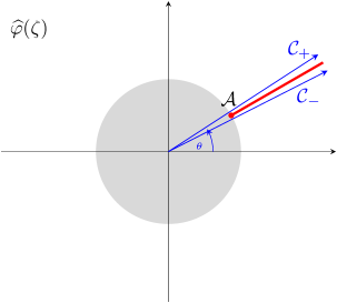
Figure 2.1: The lateral Borel resummations which sandwich a Stokes ray that pass through the singular point $\mathcal{A}$.

All resurgent series form an algebra, and the analytic formula (2.7) can be represented alternatively as an algebraic operator in the algebra of resurgent series. Introducing Stokes automorphism $\mathfrak{S}_{\theta}$ associated to the Stokes ray $\rho_{\theta}$

$$s_{\theta_{+}}=s_{\theta_{-}}\circ\mathfrak{S}_{\theta}$$ (2.8)

so that

$$\mathfrak{S}_{\theta}\varphi(z)=\varphi(z)+\sum_{k=1}^{\infty}\mathsf{s}_{kA}{\rm e}^{-k\mathcal{A}/z}\varphi^{(k\mathcal{A})}(z),$$ (2.9)

then $\mathfrak{S}_{\theta}$ is, as its name suggests, an automorphism so that for two power series $\varphi,\psi$

$$\mathfrak{S}_{\theta}(\varphi(z)\psi(z))=\mathfrak{S}_{\theta}\varphi(z)\mathfrak{S}_{\theta}\psi(z).$$ (2.10)

Another even more powerful way to encode the formula (2.7) is to introduce the alien derivatives $\stackrel{{\scriptstyle\raisebox{-0.69318pt}{$\scriptscriptstyle\bullet$}}}{{\Delta}}_{\raisebox{-0.69318pt}[3.01389pt][0.0pt]{$\scriptstyle k\mathcal{A}$}}$ associated to each Borel singularity related to the Stokes automorphism $\mathfrak{S}_{\theta}$ by

$$\mathfrak{S}_{\theta}=\exp\left(\sum_{k=1}^{\infty}\raisebox{0.99025pt}{ {$\stackrel{{\scriptstyle\raisebox{-0.69318pt}{$\scriptscriptstyle\bullet$}}}{{\Delta}}_{\raisebox{-0.69318pt}[3.01389pt][0.0pt]{$\scriptstyle k\mathcal{A}$}}$}}\right).$$ (2.11)

Upon acting on the series $\varphi$, one has

$$\raisebox{0.99025pt}{ {$\stackrel{{\scriptstyle\raisebox{-0.69318pt}{$\scriptscriptstyle\bullet$}}}{{\Delta}}_{\raisebox{-0.69318pt}[3.01389pt][0.0pt]{$\scriptstyle k\mathcal{A}$}}$}}\varphi(z)=\mathsf{S}_{k\mathcal{A}}\varphi^{(k\mathcal{A})}(z),$$ (2.12)

where the constants $\mathsf{S}_{k\mathcal{A}}$ are Stokes constants, and they are combinatoric combinations of $\mathsf{s}_{k\mathcal{A}}$. More importantly, it can be proved that $\mathfrak{S}_{\theta}$ are proper derivations, in the sense that they satisfy the following properties

• Leibniz rule: if $\varphi,\psi$ are two power series

  $$\raisebox{0.99025pt}{ {$\stackrel{{\scriptstyle\raisebox{-0.69318pt}{$\scriptscriptstyle\bullet$}}}{{\Delta}}_{\raisebox{-0.69318pt}[3.01389pt][0.0pt]{$\scriptstyle\mathcal{A}$}}$}}(\varphi(z)\psi(z))=\psi(z)\raisebox{0.99025pt}{ {$\stackrel{{\scriptstyle\raisebox{-0.69318pt}{$\scriptscriptstyle\bullet$}}}{{\Delta}}_{\raisebox{-0.69318pt}[3.01389pt][0.0pt]{$\scriptstyle\mathcal{A}$}}$}}\varphi(z)+\varphi(z)\raisebox{0.99025pt}{ {$\stackrel{{\scriptstyle\raisebox{-0.69318pt}{$\scriptscriptstyle\bullet$}}}{{\Delta}}_{\raisebox{-0.69318pt}[3.01389pt][0.0pt]{$\scriptstyle\mathcal{A}$}}$}}\psi(z).$$ (2.13)

• Chain rule: if $\psi(x,z)$ is a parametric power series in $z$ with an auxiliary parameter $x$, and $\psi(z)$ another power series in $z$

  $$\raisebox{0.99025pt}{ {$\stackrel{{\scriptstyle\raisebox{-0.69318pt}{$\scriptscriptstyle\bullet$}}}{{\Delta}}_{\raisebox{-0.69318pt}[3.01389pt][0.0pt]{$\scriptstyle\mathcal{A}$}}$}}\varphi(\psi(z),z)=\raisebox{0.99025pt}{ {$\stackrel{{\scriptstyle\raisebox{-0.69318pt}{$\scriptscriptstyle\bullet$}}}{{\Delta}}_{\raisebox{-0.69318pt}[3.01389pt][0.0pt]{$\scriptstyle\mathcal{A}$}}$}}\varphi(x,z)\big{|}_{x=\psi(z)}+\partial_{x}\varphi(x,z)\raisebox{0.99025pt}{ {$\stackrel{{\scriptstyle\raisebox{-0.69318pt}{$\scriptscriptstyle\bullet$}}}{{\Delta}}_{\raisebox{-0.69318pt}[3.01389pt][0.0pt]{$\scriptstyle\mathcal{A}$}}$}}\psi(z)$$ (2.14)

• Commutation relation:

  $$[\raisebox{0.99025pt}{ {$\stackrel{{\scriptstyle\raisebox{-0.69318pt}{$\scriptscriptstyle\bullet$}}}{{\Delta}}_{\raisebox{-0.69318pt}[3.01389pt][0.0pt]{$\scriptstyle\mathcal{A}$}}$}},\partial_{x}]=[\raisebox{0.99025pt}{ {$\stackrel{{\scriptstyle\raisebox{-0.69318pt}{$\scriptscriptstyle\bullet$}}}{{\Delta}}_{\raisebox{-0.69318pt}[3.01389pt][0.0pt]{$\scriptstyle\mathcal{A}$}}$}},\partial_{z}]=0.$$ (2.15)

  Thus $\stackrel{{\scriptstyle\raisebox{-0.69318pt}{$\scriptscriptstyle\bullet$}}}{{\Delta}}_{\raisebox{-0.69318pt}[3.01389pt][0.0pt]{$\scriptstyle\mathcal{A}$}}$ is a derivation independent of $\partial_{x}$ and $\partial_{z}$.

2.2 Resurgent structure of topological string

Consider topological string with the target space a non-compact Calabi–Yau threefold $X$. Let the number of linearly independent compact 2-cycles and compact 4-cycles be $b_{2}$ and $b_{4}$ respectively. We collect the complexified Kahler moduli of 2-cycles $t^{i}$ ($i=1,\ldots,b_{2}$) and of 4-cycles $t_{D,\ell}$ ($\ell=1,\ldots,b_{4}$) in a vector

$$\underline{\Pi}=\left(\begin{array}[]{c}\underline{t}_{D}\\ \underline{t}\\ 1\end{array}\right).$$ (2.16)

where the last entry can be regarded as the trivial Kahler modulus of a point. In general $b_{2}\geq b_{4}$, and if $b_{2}>b_{4}$, we can make the distinction of $b_{4}$ linear combinations of $t^{i}$ associated to 2-cycles that intersect with compact 4-cycles, and another $b_{2}-b_{4}$ linear combinations of $t^{i}$ associated to 2-cycles that have zero intersection numbers with compact 4-cycles. These linear combinations are called true moduli and mass parameters, denoted by $t_{*}^{\ell}$ and $t_{*}^{k+b_{4}}=m^{k}$ ($\ell=1,\ldots,b_{4}$, $k=1,\ldots b_{2}-b_{4}$) and we call the corresponding 2-cycles gauge 2-cycles and flavor 2-cycles, as they are related to Coulomb moduli and flavor masses in the associated field theory. From superstring theory point of view, the Kahler moduli in the vector $\underline{\Pi}$ are also interpreted as the central charges of D4-, D2-, and D0-branes supported on these cycles.

The moduli space of the Calabi–Yau threefold enjoy special properties known as the special geometry relations, among which we can define the prepotential $\mathcal{F}_{0}$, a function of $t^{i}$, so that

$$t_{D,\ell}=\sum_{i=1}^{b_{2}}C^{i}_{\ell}\frac{\partial\mathcal{F}_{0}}{\partial t^{i}},\quad\ell=1,\ldots,b_{4},$$ (2.17)

where $C^{i}_{\ell}$ are entries of the integer valued $b_{2}\times b_{4}$ intersection matrix between compact 2-cycles and compact 4-cycles. $\mathcal{F}_{0}$ is the genus zero component of the free energy, and higher genus free energies $\mathcal{F}_{g}$ can be constructed by coupling the worldsheet theory to gravity. Mathematically, the free energies are defined as the generating function of Gromov-Witten invariants, the counting of stable holomorphic maps from genus $g$ Riemann surfaces to 2-cycles in the Calabi–Yau $X$, i.e.

$$\mathcal{F}_{g}({\underline{t}})=\sum_{\beta\in H_{2}(X)}N_{g,\beta}{\rm e}^{-t(\beta)},$$ (2.18)

where $t(\beta)$ is the complexified volume of the 2-cycle $\beta$. Collectively, the perturbative free energy of topological string is

$$\mathcal{F}^{(0)}_{\text{top}}({\underline{t}},g_{s})=\sum_{g\geq 0}\mathcal{F}_{g}({\underline{t}})g_{s}^{2g-2}.$$ (2.19)

Through mirror symmetry, the components of the vector $\underline{\Pi}$ are identified with complex structure moduli of the mirror threefold $Y$, which are periods of the holomorphic $(3,0)$ form over integral 3-cycles in $Y$, or equivalently with periods of the canonical 1-form over integral 1-cycles in the mirror curve $\Sigma$ that the threefold $Y$ can reduce to. Hence $\underline{\Pi}$ is also called the period vector. The distinction between $t^{i}$ and $t_{D,\ell}$ corresponds to a choice of symplectic basis of $H_{1}(\Sigma)$ consisting of A-cycles and B-cycles so that the oriented intersection is

$$A^{i}\cap B_{\ell}=C^{i}_{\ell}.$$ (2.20)

And $t^{i},t_{D,\ell}$ are correspondingly called the A- and B-periods. Such a choice is not unique, and a different choice of A- and B-cycles, known as a different frame, leads to different A- and B-periods. The frame given by (2.17) is called the large radius frame. We denote A- and B-periods in a generic frame $\Gamma$ by

$$t^{\Gamma,i},\quad t^{\Gamma}_{D,\ell},\quad i=1,\ldots,b_{2},\quad\ell=1,\ldots,b_{4},$$ (2.21)

and the special geometry relation (2.17) becomes accordingly

$$t^{\Gamma}_{D,\ell}=\sum_{i=1}^{b_{2}}{{C^{\Gamma}}}^{i}_{\ell}\frac{\partial{\mathcal{F}^{\Gamma}}_{0}}{\partial t^{\Gamma,i}},\quad\ell=b_{4},$$ (2.22)

where ${{C^{\Gamma}}}^{i}_{\ell}$ is the intersection matrix of A- and B-cycles in frame $\Gamma$. Clearly, the prepotential ${\mathcal{F}^{\Gamma}}_{0}$, as well as the genus $g$ free enegies ${\mathcal{F}^{\Gamma}}_{g}$, depend on the choice of frame $\Gamma$. Although this is not always the case, throughout our paper, we choose frames so that A- and B-cycles are integral cycles, so that changing a frame amounts to a symplectic transformation in $Sp(b_{3}(Y),\mathbb{Z})$ of the interal periods. To find how free energies change across different frames, it was noted in Aganagic:2006wq that free energies ${\mathcal{F}^{\Gamma}}_{g}$ for $g\geq 2$ and $\exp({\mathcal{F}^{\Gamma}}_{1})$ are almost holomorphic modular forms, whose modular parameter is

$$\tau^{\Gamma}_{\ell m}=\sum_{i,j=1}^{b_{2}}{{C^{\Gamma}}}^{i}_{\ell}{{C^{\Gamma}}}^{j}_{m}\frac{\partial^{2}{\mathcal{F}^{\Gamma}}_{0}}{\partial{t^{\Gamma}}^{i}\partial{t^{\Gamma}}^{j}},\quad\ell,m=1,\ldots b_{4},$$ (2.23)

and a change of frame is equivalent to a modular transformation of these almost holomorphic modular forms.

In the remainder of this section, we will drop the superscript $\Gamma$ for frame to reduce the notational clutter. Regardless of which frame one is at, the genus $g$ free energy $\mathcal{F}_{g}({\underline{t}})$ is a well-defined function, while the perturbative series $\mathcal{F}^{(0)}_{\text{top}}({\underline{t}},g_{s})$ is a divergent series of Gevrey-1 type Marino:2006hs ; Marino:2007te

$$\mathcal{F}_{g}({\underline{t}})\sim(2g)!$$ (2.24)

and therefore there should be non-perturbative corrections which can be analysed by resurgence techniques. It has been found that the locations of singularities of the Borel transform always coincide with classical integral periods up to normalisation Pasquetti2010 ; Aniceto2012 ; Couso-Santamaria2016 ; Couso-Santamaria2015 ; Alim:2021mhp ; Grassi:2022zuk ; Gu:2022sqc . More precisely,

$$\mathcal{A}_{(\underline{p},\underline{q},\underline{s})}=\aleph(\underline{p}\cdot\underline{t}_{D}+\underline{q}\cdot\underline{t}+s),$$ (2.25)

where $\aleph=4\pi^{2}{\mathsf{i}}$, $p^{\ell},q_{i},s$ are certain integer numbers. We will not discuss the cases with $p^{\ell}=q_{i}=0$ as they are trivial.

The alien derivative of the free energy $\mathcal{F}^{(0)}({\underline{t}},g_{s})$ at a singular point $\mathcal{A}$ is proportional to the instanton amplitude associated to this singularity. In particular, if we have a sequence of singular points $k\mathcal{A}$, $k=1,2,\ldots$ along a Stokes ray $\rho_{\text{arg}\mathcal{A}}$, and let us denote the instanton amplitude at the singularity $k\mathcal{A}$ by $\mathcal{F}^{(k)}$, the alien derivatives at these singular points read Gu:2022sqc ; Gu:2023mgf

$$\raisebox{0.99025pt}{ {$\stackrel{{\scriptstyle\raisebox{-0.69318pt}{$\scriptscriptstyle\bullet$}}}{{\Delta}}_{\raisebox{-0.69318pt}[3.01389pt][0.0pt]{$\scriptstyle k\mathcal{A}$}}$}}\mathcal{F}^{(0)}_{\text{top}}({\underline{t}},g_{s})=\frac{{\mathsf{i}}}{2\pi}\mathsf{S}_{k\mathcal{A}}^{\text{top}}\mathcal{F}^{(k)}_{\text{top}}({\underline{t}},g_{s}).$$ (2.26)

Here, both the perturbative free energy and the instanton amplitudes depend on the holomorphic frame of evaluation. In particular, the expression of the instanton amplitude depends greatly on the type of frame. If a frame, known as an A-frame, is chosen such that $\mathcal{A}=\mathcal{A}_{(\underline{p},\underline{q},\underline{s})}$ is an A-period, i.e. $p^{\ell}=0$, then the instanton amplitude simplifies greatly and we have

$$\mathcal{F}^{(k)}_{\text{top},\mathcal{A}}({\underline{t}},g_{s})=\left(\frac{1}{k^{2}}+\frac{\mathcal{A}}{kg_{s}}\right){\rm e}^{-k\mathcal{A}/g_{s}},$$ (2.27)

where the subscript $\mathcal{A}$ refers to the A-frame. If we are not in an A-frame, the instanton amplitude has more complicated form, but we will not need them here.

The Stokes constants $\mathsf{S}_{k\mathcal{A}}^{\text{top}}$ are very interesting, as it was found empirically in Gu:2022sqc ; Gu:2023mgf that they satisfy certain intriguing properties. They are integers, and they seem to be frame independent as well as the same for all the singular points $k\mathcal{A}$. Among these properties, the frame independence may be due to the following reason. It is known that the holomorphic and frame dependent free energies $\mathcal{F}_{g}({\underline{t}})$ can be lifted to anholomorphic and frame independent free energies $F_{g}({\underline{t}},\bar{{\underline{t}}})$ Bershadsky:1993cx ; Bershadsky:1993ta , and choosing a frame is done by sending $\bar{{\underline{t}}}$ to some fixed value, which can be interpreted as choosing a different gravitational background Witten:1993ed . We speculate that (2.26) also holds when both sides are lifted to anholomorphic amplitudes

$$\raisebox{0.99025pt}{ {$\stackrel{{\scriptstyle\raisebox{-0.69318pt}{$\scriptscriptstyle\bullet$}}}{{\Delta}}_{\raisebox{-0.69318pt}[3.01389pt][0.0pt]{$\scriptstyle k\mathcal{A}$}}$}}F^{(0)}_{\text{top}}({\underline{t}},\bar{{\underline{t}}},g_{s})=\frac{{\mathsf{i}}}{2\pi}\mathsf{S}_{k\mathcal{A}}^{\text{top}}F^{(k)}_{\text{top}}({\underline{t}},\bar{{\underline{t}}},g_{s}).$$ (2.28)

The frame independence of the Stokes constants is then equivalent to the conjecture that they are background independent.

The purpose of this note is to uncover the nature of the Stokes constants $\mathsf{S}_{k\mathcal{A}}^{\text{top}}$ by relating them to the Stokes constants of the refined free energy in the Nekrasov–Shatashvili limit. The perturbative free energy of topological string can be refined to

$$\mathcal{F}^{(0)}({\underline{t}},\epsilon_{1},\epsilon_{2})=\sum_{n,g\geq 0}(\epsilon_{1}+\epsilon_{2})^{2n}(\epsilon_{1}\epsilon_{2})^{g-1}\mathcal{F}_{n,g}({\underline{t}}),$$ (2.29)

which reduces to the conventional topological string in the limit $\epsilon_{1}=-\epsilon_{2}={\mathsf{i}}g_{s}$

$$\mathcal{F}^{(0)}_{\text{top}}({\underline{t}},g_{s})=\mathcal{F}^{(0)}({\underline{t}},{\mathsf{i}}g_{s},-{\mathsf{i}}g_{s}).$$ (2.30)

Another interesting limit we can take is the Nekrasov–Shatashvili limit

$$\mathcal{F}^{(0)}_{\text{NS}}({\underline{t}},\hbar)=\lim_{\epsilon_{2}\rightarrow 0}{\mathsf{i}}\epsilon_{2}\mathcal{F}^{(0)}({\underline{t}},{\mathsf{i}}\hbar,\epsilon_{2})=:\sum_{n\geq 0}\mathcal{F}^{\text{NS}}_{n}({\underline{t}})\hbar^{2n-1}.$$ (2.31)

The components $\mathcal{F}^{\text{NS}}_{n}({\underline{t}})$ are also almost holomorphic modular forms and they transform accordingly in a change of frame as well.

The NS free energies are also Gevrey-1 series in $\hbar$, and we can similarly perform resurgence analysis. We find the singularities of the Borel transform are also located in (2.25) Gu:2022fss . The alien derivatives of NS free energy at such a singularity is found to be

$$\raisebox{0.99025pt}{ {$\stackrel{{\scriptstyle\raisebox{-0.69318pt}{$\scriptscriptstyle\bullet$}}}{{\Delta}}_{\raisebox{-0.69318pt}[3.01389pt][0.0pt]{$\scriptstyle k\mathcal{A}$}}$}}\mathcal{F}^{(0)}_{\text{NS}}({\underline{t}},\hbar)=\frac{{\mathsf{i}}\hbar}{2\pi}\mathsf{S}_{\mathcal{A}}^{\text{NS}}\mathcal{F}^{(k)}_{\text{NS}}.$$ (2.32)

Both perturbative and instantonic free energies are frame dependent. In the case where $\mathcal{A}$ is an A-period, i.e. in an A-frame, one finds Gu:2022fss

$$\mathcal{F}^{(\ell)}_{\text{NS},\mathcal{A}}=\frac{(-1)^{k-1}}{k^{2}}{\rm e}^{-k\mathcal{A}/\hbar}.$$ (2.33)

In the cases where $\mathcal{A}$ is not an A-period, i.e. $\mathcal{A}$ is given by (2.25) with $\underline{p}\neq\underline{0}$, we can shift the definition of prepotential $\mathcal{F}_{0}$ so that

$$\mathcal{A}=-\frac{1}{2\pi}\sum_{i=1}^{b_{2}}\sum_{\ell=1}^{b_{4}}\frac{\partial\mathcal{F}_{0}}{\partial t^{i}}C^{i}{}_{\ell}p^{\ell}$$ (2.34)

Then the instanton ampitudes of NS free energy are Gu:2022fss

$$\mathcal{F}^{(\ell)}_{\text{NS}}=\frac{(-1)^{k-1}}{k^{2}}{\rm e}^{-k\mathcal{G}({\underline{t}},\hbar)/\hbar},$$ (2.35)

where the quantity $\mathcal{G}({\underline{t}},\hbar)$ is defined by

$$\mathcal{G}({\underline{t}},\hbar)=-\frac{\hbar}{2\pi}\sum_{i=1}^{b_{2}}\sum_{\ell=1}^{b_{4}}\frac{\partial\mathcal{F}^{(0)}_{\text{NS}}({\underline{t}},\hbar)}{\partial t^{i}}C^{i}{}_{\ell}p^{\ell}.$$ (2.36)

Yet again, it was found empirically in Gu:2022sqc that the Stokes constants $\mathsf{S}_{\mathcal{A}}^{\text{NS}}$ are integers, the same for all $k\mathcal{A}$, and seem to be frame independent. The forms of the alien derivatives (2.32) and the properties of the Stokes constants $\mathsf{S}_{\mathcal{A}}^{\text{NS}}$ have profound consequences. As pointed out in Gu:2022fss (see also DelMonte:2022kxh ) and will be reviewed in Appendix A, they imply, together with the Stokes transformation properties of Wilson loop amplitudes, that the quantum periods satisfy the DDP type of formulas for Stokes automorphism Dillinger:1993 ; Delabaere19971:exact ; Delabaere1999 , so that the Stokes constants of quantum periods can be identified with BPS invariants. More importantly, the Stokes constants $\mathsf{S}_{\mathcal{A}}^{\text{NS}}$ are identified with those of quantum periods Gu:2022fss , so that $\mathsf{S}_{\mathcal{A}}^{\text{NS}}$ themselves are given by BPS invariants. More precisely, the coefficients $(\underline{p},\underline{q},s)$ in the composition of $\mathcal{A}$ in (2.25) are brane charges. For instance in the large radius frame, $(\underline{p},\underline{q},s)$ are respectively the D4-, D2-, and D0-brane charges. $\mathsf{S}_{\mathcal{A}}^{\text{NS}}$ is then the counting of BPS states of stable D-brane bound states with brane charges $\gamma(\mathcal{A})=(\underline{p},\underline{q},s)$; in other words,

$$\mathsf{S}_{\mathcal{A}}^{\text{NS}}=\Omega(\gamma(\mathcal{A})).$$ (2.37)

We will show in Section 4 that the Stokes constants $\mathsf{S}_{\mathcal{A}}^{\text{top}}$ of unrefined free energies coincide up to a sign with $\mathsf{S}_{\mathcal{A}}^{\text{NS}}$ of NS free energies as in (4.9).

3 Blowup equations of refined topological string

3.1 Blowup equations in large radius frame

It was conjecturd Gu:2017ccq ; Huang:2017mis based on Grassi:2016nnt ; Sun2016 and checked in many examples that the blowup equations for supersymmetric gauge theories Nakajima:2003pg ; Nakajima:2005fg ; Nakajima:2009qjc ; Gottsche:2006bm can be generalised and are satisfied by free energies of topological string on a local Calabi–Yau threefold $X$. And it was pointed out in Huang:2017mis that blowup equations can be used to solve D2-D0 type BPS invariants. This line of research was later expanded in Gu:2018gmy ; Gu:2019dan ; Gu:2019pqj ; Gu:2020fem ; Kim:2019uqw ; Kim:2020hhh ; Kim:2021gyj ; Kim:2023glm ; Wang:2023zcb . See also related works in Nekrasov:2020qcq ; Shchechkin:2020ryb ; Bershtein:2018zcz ; Jeong:2020uxz ; Sun:2021lsq . The blowup equations will play a crucial role for relating the Stokes constants of unrefined and NS free energies of topological string.

Let us work in the large radius frame. The number of linearly independent compact 2-cycles and 4-cycles in Calabi–Yau threefold $X$ are respectively $b_{2}$ and $b_{4}$. Denote by $\underline{C}$ the $b_{2}\times b_{4}$ intersection matrix between compact 2-cycles and 4-cycles. The complex Kahler moduli of compact 2-cycles are ${\underline{t}}$. Then it was conjectured that there exist $b_{2}$-dimensional integer valued vectors $\underline{r}$ satisfying the checkerboard pattern conditions, also known as flux quantisation conditions, for non-vanishing D2-D0 brane BPS invariants $N^{\underline{d}}_{j_{L},j_{R}}$

$$2j_{L}+2j_{R}+1\equiv\underline{r}\cdot\underline{d}\quad\text{mod}\;2,\quad N^{\underline{d}}_{j_{L},j_{R}}\neq 0,$$ (3.1)

such that the refined free energy of topological string satifies the so-called blowup equations,

$$\Lambda(\underline{m},\epsilon_{1},\epsilon_{2})=\sum_{\underline{n}\in\mathbb{Z}^{b_{4}}}(-1)^{|\underline{n}|}\exp\left(\mathcal{F}_{\text{ref}}({\underline{t}}+\frac{\epsilon_{1}}{2\pi{\mathsf{i}}}{\underline{R}},\epsilon_{1},\epsilon_{2}-\epsilon_{1})+\mathcal{F}_{\text{ref}}({\underline{t}}+\frac{\epsilon_{2}}{2\pi{\mathsf{i}}}{\underline{R}},\epsilon_{1}-\epsilon_{2},\epsilon_{2})-\mathcal{F}_{\text{ref}}({\underline{t}},\epsilon_{1},\epsilon_{2})\right)$$ (3.2)

where $|\underline{n}|=n_{1}+\ldots+n_{b_{4}}$, and

$$\underline{R}=\underline{C}\cdot\underline{n}+\frac{\underline{r}}{2}.$$ (3.3)

Here the vector $\underline{r}$ is in addition subject to the equivalence relation

$$\underline{r}\sim\underline{r}+2\underline{C}\cdot\underline{n}^{\prime},\quad\underline{n}^{\prime}\in\mathbb{Z}^{b_{4}},$$ (3.4)

as (3.2) does not change under this transformation. Besides the crucial factor $\Lambda(\underline{m},\epsilon_{1},\epsilon_{2})$ depends not on all the Kahler moduli but only the mass parameters. We will be interested in the special cases where $\Lambda$ vanishes identically. These are called vanishing blowup equations.

One subtlety concerning the blowup equations as claimed in Grassi:2016nnt ; Gu:2017ccq ; Huang:2017mis is that the refined free energies that appear in (3.2) should be twisted in the sense that

$$\mathcal{F}_{\text{ref}}\rightarrow\widehat{\mathcal{F}}_{\text{ref}}({\underline{t}},\epsilon_{1},\epsilon_{2})=\mathcal{F}_{\text{ref}}^{\text{pert}}({\underline{t}},\epsilon_{1},\epsilon_{2})+\mathcal{F}_{\text{ref}}^{\text{inst}}({\underline{t}}+\frac{{\underline{B}}}{2},\epsilon_{1},\epsilon_{2}),$$ (3.5)

where ${\underline{B}}$, known as the B-field, is a $\mathbb{Z}_{2}$ valued $b_{2}$-dimensional vector defined by

$${\underline{B}}\equiv\underline{r}\;\text{mod}\;(\mathbb{Z}_{2})^{b_{2}},$$ (3.6)

The twisted free energy was introduced so that when a gauge theory description is available it coincides with the logarithm of the Nekrasov partition funtion. Here $F_{\text{ref}}^{\text{inst}}$ is the instanton contributions, while $F_{\text{ref}}^{\text{pert}}$ is the sum of classical and 1-loop contributions and it is given collectively by

$$\mathcal{F}_{\text{ref}}^{\text{pert}}({\underline{t}},\epsilon_{1},\epsilon_{2})=\frac{1}{\epsilon_{1}\epsilon_{2}}\left(\frac{1}{6}\sum_{i,j,k}a_{ijk}t_{i}t_{j}t_{k}+4\pi^{2}\sum_{i=1}^{s}b_{i}^{\text{NS}}t_{i}\right)+\sum_{i=1}^{s}b_{i}t_{i}-\frac{(\epsilon_{1}+\epsilon_{2})^{2}}{\epsilon_{1}\epsilon_{2}}\sum_{i=1}^{s}b_{i}^{\text{NS}}t_{i}.$$ (3.7)

where $a_{ijk}$ are triple intersection numbers of divisors in $X$ and $b_{i}^{\text{NS}},b_{i}$ are some other intersection numbers. The three terms on the right hand side in (3.7) come from $\mathcal{F}_{(0,0)},\mathcal{F}_{(0,1)},\mathcal{F}_{(1,0)}$ respectively. As it stands, $\mathcal{F}_{\text{ref}}^{\text{pert}}$ defined in (3.7) does not have quadratic contributions and it is calculated from the special geometry relation (2.17) using the Frobenius basis of periods. If, however, we integrate the special geometry relation (2.17) using the integral basis of periods as we do in this paper, we would have that

$$\mathcal{F}_{\text{ref}}^{\text{pert,Frob}}({\underline{t}}-\frac{{\underline{B}}}{2},\epsilon_{1},\epsilon_{2})=\mathcal{F}_{\text{ref}}^{\text{pert,int'l}}({\underline{t}},\epsilon_{1},\epsilon_{2})+\frac{1}{\epsilon_{1}\epsilon_{2}}\mathcal{O}({\underline{t}})+\mathcal{O}(1)+\frac{(\epsilon_{1}+\epsilon_{2})^{2}}{\epsilon_{1}\epsilon_{2}}\mathcal{O}(1),$$ (3.8)

with an appropriate representation of $B$. As we will later see in (3.17), the blowup equations only depend on $\mathcal{F}_{(0,0)},\mathcal{F}_{(0,1)},\mathcal{F}_{(1,0)}$ through

$$\partial_{t}^{n\geq 2}\mathcal{F}_{(0,0)},\;\partial_{t}^{n\geq 1}\mathcal{F}_{(0,1)},\;\partial_{t}^{n\geq 1}\mathcal{F}_{(1,0)}$$ (3.9)

so that the difference in (3.8) is irrelevant. In light of this relation, we can use the blowup equations (3.2) with the understanding that we can use refined free energies of topological string based on an integral basis of periods for the moduli without twist after making the shift

$${\underline{t}}\rightarrow{\underline{t}}-{\underline{B}}/2.$$ (3.10)

Let us illustrate (3.8) with the simple example of the local $\mathbb{P}^{2}$ model. This model has a one dimensional moduli space $\mathcal{M}$ parametrised by a global modulus $z$. In the large radius frame, the integral periods are Aganagic:2006wq ; Haghighat:2008gw

$$\underline{\Pi}=\begin{pmatrix}t_{D}\\ t\\ 1\end{pmatrix}=\begin{pmatrix}1&-\frac{1}{2}&\frac{1}{4}\\ 0&1&0\\ 0&0&1\end{pmatrix}\cdot\underline{\Pi}_{0}$$ (3.11)

where $\underline{\Pi}_{0}$ is the Frobenius basis given by

$$\underline{\Pi}_{0}=\begin{pmatrix}X^{(1,1)}\\ X^{(1)}\\ 1\end{pmatrix}=\begin{pmatrix}\frac{1}{2(2\pi{\mathsf{i}})^{2}}\left(\log(z)^{2}+2\sigma_{1}(z)\log(z)+\sigma_{2}(z)\right)\\ \frac{1}{2\pi{\mathsf{i}}}\left(\log(z)+\sigma_{1}(z)\right)\\ 1\end{pmatrix}$$ (3.12)

where

$$\sigma_{1}(z)= \sum_{j\geq 1}3\frac{(3j-1)!}{(j!)^{3}}(-z)^{j},$$ (3.13a)

$$\sigma_{2}(z)= \sum_{j\geq 1}\frac{18}{j!}\frac{(3j-1)!}{(j!)^{3}}(-z)^{j}\left(\psi(3j)-\psi(j+1)\right),$$ (3.13b)

with $\psi$ being digamma function. The special geoemtry relation is Aganagic:2006wq

$$t_{D}=-3(2\pi{\mathsf{i}})^{-3}\partial_{t}\mathcal{F}_{0}(t).$$ (3.14)

The prepotential obtained by integrating the special geometry relation using the integral periods $t_{D}$ and $t$ is

$$\mathcal{F}_{0}^{\text{int'l}}(t)=-\frac{t^{3}}{18}+\frac{t^{2}}{12}-\frac{t}{12}+\mathcal{O}(1)$$ (3.15)

while the prepotential obtained by replacing $t_{D},t$ with the Frobenius periods $X^{(1,1)},X^{(1)}$, as practised in Huang:2017mis , is

$$\mathcal{F}_{0}^{\text{Frob}}(t)=-\frac{t^{3}}{18}+\mathcal{O}(1)$$ (3.16)

and they satisfy (3.8) after taking into account that we can take $B=1$ in local $\mathbb{P}^{2}$ Huang:2017mis .

3.2 Blowup equations in a generic integral frame

The blowup equations (3.2) are formulated for free energies in the large radius frame. Nevertheless, it is possible to change the frame and write down the blowup equations in other integral frames as well. One way of doing this is using the anholomorphic blowup equations proposed in Sun:2021lsq and choosing the appropriate holomorphic limit. Another way is expand the blowup equations in terms of $\epsilon_{1}+\epsilon_{2}$ and $\epsilon_{1}\epsilon_{2}$

$${\rm e}^{\mathcal{F}_{(0,1)}-\mathcal{F}_{(1,0)}} \sum_{\underline{n}\in\mathbb{Z}^{b_{4}}}(-1)^{|\underline{n}|}{\rm e}^{-\frac{1}{2}R^{2}\mathcal{F}^{\prime\prime}_{(0,0)}}(1+(\epsilon_{1}+\epsilon_{2})(R\mathcal{F}^{\prime}_{(0,1)}+R\mathcal{F}^{\prime}_{(1,0)}-\frac{1}{6}R^{3}\mathcal{F}^{\prime\prime\prime}_{(0,0)}+\ldots)$$

$$= \Lambda_{(0,0)}(\underline{m})+(\epsilon_{1}+\epsilon_{2})\Lambda_{(1,0)}(\underline{m})+\ldots.$$ (3.17)

Here we use the notation

$$R^{k}\mathcal{F}^{(k)}_{(n,g)}=\sum_{i_{1},\ldots,i_{k}}(2\pi{\mathsf{i}})^{-k}R_{i_{1}}\ldots R_{i_{k}}\partial_{t_{i_{1}}}\ldots\partial_{t_{i_{k}}}\mathcal{F}_{(n,g)}({\underline{t}})$$ (3.18)

and $\Lambda_{(n,g)}$ are components of $\Lambda(\underline{m},\epsilon_{1},\epsilon_{2})$ through the expansion

$$\Lambda(\underline{m},\epsilon_{1},\epsilon_{2})=\sum_{n,g\geq 0}\Lambda_{(n,g)}(\epsilon_{1}+\epsilon_{2})^{n}(\epsilon_{1}\epsilon_{2})^{g}$$ (3.19)

At each order of $\epsilon_{1}+\epsilon_{2}$ and $\epsilon_{1}\epsilon_{2}$, the left hand side is a linear sum of

$$\sum_{\underline{n}\in\mathbb{Z}^{b_{4}}}(-1)^{|\underline{n}|}R^{k}{\rm e}^{-\frac{1}{2}R^{2}\mathcal{F}^{\prime\prime}_{(0,0)}}$$ (3.20)

which are theta constants with modulus $\tau\propto\mathcal{F}^{\prime\prime}_{(0,0)}$ and its higher dimensional generalisations. The coefficients of the linear sum are products of ${\rm e}^{\mathcal{F}_{(0,1)}-\mathcal{F}_{(1,0)}}$ and $\mathcal{F}^{(k)}_{(n,g)}$ which are almost holomorphic modular forms of $\tau$. The identity (3.17) at each order of $\epsilon_{1}+\epsilon_{2}$ and $\epsilon_{1}\epsilon_{2}$ expansion is an equation of almost holomorphic modular forms, and they have been checked for various examples in Huang:2017mis . A frame transformation is then akin to a modular transformation at each order of (3.17) and they can be reassembled into the blowup equation in the corresponding new frame.

The blowup equation in an arbitrary integral frame takes a form similar to (3.2),

$${\Lambda^{\Gamma}}(\underline{m},\epsilon_{1},\epsilon_{2})= \sum_{\underline{n}\in\mathbb{Z}^{b_{4}}}(-1)^{|\underline{n}|}\exp\Big{(}{\mathcal{F}^{\Gamma}}_{\text{ref}}({\underline{t}^{\Gamma}}+\frac{\epsilon_{1}}{2\pi{\mathsf{i}}}{\underline{R}^{\Gamma}},\epsilon_{1},\epsilon_{2}-\epsilon_{1})+{\mathcal{F}^{\Gamma}}_{\text{ref}}({\underline{t}^{\Gamma}}+\frac{\epsilon_{2}}{2\pi{\mathsf{i}}}{\underline{R}^{\Gamma}},\epsilon_{1}-\epsilon_{2},\epsilon_{2})$$

$$-{\mathcal{F}^{\Gamma}}_{\text{ref}}({\underline{t}^{\Gamma}},\epsilon_{1},\epsilon_{2})\Big{)},$$ (3.21)

with

$${\underline{R}^{\Gamma}}={\underline{\mathcal{C}}}^{\Gamma}\cdot\underline{n}+{\underline{r}^{\Gamma}}/2.$$ (3.22)

The ingredient ${\underline{R}^{\Gamma}}$ including its coefficients ${\underline{\mathcal{C}}}^{\Gamma}$ and ${\underline{r}^{\Gamma}}$ as well as ${\Lambda^{\Gamma}}(\underline{m},\epsilon_{1},\epsilon_{2})$ may change over different frames. We will only be interested in vanishing blowup equations so the change of ${\Lambda^{\Gamma}}(\underline{m},\epsilon_{1},\epsilon_{2})$ is trivial as it stays zero across all frames.

On the other hand, ${\underline{\mathcal{C}}}^{\Gamma}$ and ${\underline{r}^{\Gamma}}$ in ${\underline{R}^{\Gamma}}$ should change appropriately so that each component in the expansion (3.17) transform consistently under modular transformations. The properties of ${\underline{\mathcal{C}}}^{\Gamma}$ and ${\underline{r}^{\Gamma}}$ would be crucial in later sections. We will only consider frames defined by integral basis of periods, and in these cases we argue that we always have

$${\underline{\mathcal{C}}}^{\Gamma}\text{ is an \emph{integer} valued }b_{2}\times b_{4}\text{ matrix.}$$ (3.23)

Indeed the sum over $\underline{n}\in\mathbb{Z}^{b_{4}}$ is a summation over discrete magnetic flux over the exceptional divisor $\mathbb{P}^{2}$ in the spacetime $\mathbb{C}^{2}\cong\mathbb{R}^{4}$ blown up at the origin $B\mathbb{C}^{2}$ in the field theory description Nakajima:2003pg ; Nakajima:2005fg ; Gottsche:2006bm ; Nakajima:2009qjc , and each component of the flux vector is associated to an irreducible compact 4-cycle in the Calabi–Yau $X$ Grassi:2016nnt ; Gu:2017ccq ; Huang:2017mis ; Kim:2020hhh . Therefore, in the case of large radius frame where the moduli ${t^{\Gamma}}^{i}=t^{i}$ are associated with integral 2-cycles, ${\underline{\mathcal{C}}}^{\Gamma}=\underline{C}$ is defined as the integer valued intersection matrix of 2-cycles and 4-cycles. In a generic integral frame, each modulus ${t^{\Gamma}}^{i}$ is associated with either an integral 2-cycle or an integral 4-cycle. In the former case, the corresponding row of ${\underline{\mathcal{C}}}^{\Gamma}$ is the integer valued intersection numbers with 4-cycles; in the latter case, the corresponding row of ${\underline{\mathcal{C}}}^{\Gamma}$ should be the integer valued decomposition coefficients in terms of a basis of integral and irreducible 4-cycles. We emphysize that in a generic frame, ${\underline{\mathcal{C}}}^{\Gamma}$ is not identified with the intersection matrix ${\underline{C}^{\Gamma}}$ given in (2.22).

Similar to the large radius case, the vector ${\underline{r}^{\Gamma}}$ is defined up to the equivalence relation

$${\underline{r}^{\Gamma}}\sim{\underline{r}^{\Gamma}}+2{\underline{\mathcal{C}}}^{\Gamma}\cdot\underline{n}^{\prime},\quad\underline{n}^{\prime}\in\mathbb{Z}^{b_{4}}.$$ (3.24)

We also comment that even though we do not have a physics argument, the vector ${\underline{r}^{\Gamma}}$ also seems to be integer valued in an arbitrary frame defined by integral periods. We demonstrate the integrality of both ${\underline{\mathcal{C}}}^{\Gamma}$ and ${\underline{r}^{\Gamma}}$ through two examples below.

3.2.1 Local $\mathbb{P}^{2}$

We first consider the simple example of the local $\mathbb{P}^{2}$ model. The first two orders of the expansion of the vanishing blowup equations (3.21) with ${\Lambda^{\Gamma}}=0$ in terms of $\epsilon_{1}+\epsilon_{2}$ and $\epsilon_{1}\epsilon_{2}$, similar to (3.17), are

$${\Theta^{\Gamma}}_{0}({t^{\Gamma}})=0$$ (3.25a)

$${\Theta^{\Gamma}}_{1}({t^{\Gamma}})\left({\mathcal{F}^{\Gamma}}^{\prime}_{(0,1)}({t^{\Gamma}})+{\mathcal{F}^{\Gamma}}^{\prime}_{(1,0)}({t^{\Gamma}})\right)-\frac{1}{6}{\Theta^{\Gamma}}_{3}({t^{\Gamma}}){\mathcal{F}^{\Gamma}}^{\prime\prime\prime}_{(0,,0)}({t^{\Gamma}})=0,$$ (3.25b)

where ${\Theta^{\Gamma}}_{k}({t^{\Gamma}})$ are the theta constants

$${\Theta^{\Gamma}}_{k}({t^{\Gamma}})=\sum_{n\in\mathbb{Z}}(-1)^{n}(2\pi{\mathsf{i}})^{-k}({R^{\Gamma}})^{k}{\rm e}^{-\frac{1}{2}({R^{\Gamma}})^{2}{\mathcal{F}^{\Gamma}}^{\prime\prime}_{(0,0)}}.$$ (3.26)

Consider first the large radius frame, where we will drop all the superscript $\Gamma$. These two equations have been checked in Huang:2017mis . Indeed, we have

$$R=3(n+1/2)$$ (3.27)

and it is easy to see that (3.25a) is satisfied as the summand of $\Theta_{0}$ is an odd function of $n$. Furthermore, let us introduce the theta constants relevant for the local $\mathbb{P}^{2}$ model

$$a(\tau)=\theta^{3}\left[\begin{array}[]{c}\frac{1}{6}\\ \frac{1}{6}\end{array}\right](0,\tau),\;b(\tau)=\theta^{3}\left[\begin{array}[]{c}\frac{1}{6}\\ \frac{1}{2}\end{array}\right](0,\tau),\;c(\tau)=\theta^{3}\left[\begin{array}[]{c}\frac{1}{6}\\ \frac{5}{6}\end{array}\right](0,\tau),\;d(\tau)=\theta^{3}\left[\begin{array}[]{c}\frac{1}{2}\\ \frac{1}{6}\end{array}\right](0,\tau),$$ (3.28)

with

$$\theta\left[\epsilon,\epsilon^{\prime}\right](z,\tau)=\sum_{n\in\mathbb{Z}}\exp(\pi{\mathsf{i}}\tau(n+\epsilon)^{2}+2\pi{\mathsf{i}}(n+\epsilon)(z+\epsilon^{\prime}))$$ (3.29)

They have modular weight $3/2$ and enjoy the properties

$$a(-1/\tau)=\kappa_{1}\tau^{3/2}c(\tau),\quad b(-1/\tau)=\kappa_{2}\tau^{3/2}d(\tau),$$ (3.30)

where $\kappa_{1,2}$ are roots of unity. Then the free energies $\mathcal{F}_{(0,1)}(t),\mathcal{F}_{(1,0)}(t)$ are Haghighat:2008gw ; Huang:2010kf

$$\mathcal{F}_{(0,1)}(t)=-\frac{1}{6}\log(d(\tau)\eta^{3}(\tau)),\quad\mathcal{F}_{(1,0)}(t)=\frac{1}{6}\log(\eta^{3}(\tau)/d(\tau)),$$ (3.31)

where the modular parameter is

$$\tau=\frac{\partial t_{D}}{\partial t}=-3(2\pi{\mathsf{i}})^{-3}\partial^{2}_{t}\mathcal{F}_{0}.$$ (3.32)

Note that here $\mathcal{F}_{(0,1)}(t)$ is the holomorphic limit of the anholomorphic

$$F_{(0,1)}(t,\bar{t})=-\frac{1}{2}\log\tau_{2}\eta^{2}\bar{\eta}^{2}+\frac{1}{2}\log\eta/d^{1/3},$$ (3.33)

with $\tau_{2}=\operatorname{Im}\tau$. Using expressions of $\mathcal{F}_{(0,1)},\mathcal{F}_{(1,0)}$ in (3.31), (3.25b) can be integrated to

$$\sum_{n\in\mathbb{Z}}(-1)^{n}(n+\frac{1}{2}){\rm e}^{3\pi{\mathsf{i}}(n+\frac{1}{2})^{2}\tau}=\text{Const.}d(\tau)$$ (3.34)

which can be checked to high degrees of $q=\exp(2\pi{\mathsf{i}}\tau)$ expansion.

As mentioned before, the local $\mathbb{P}^{2}$ model has a one dimensional moduli space $\mathcal{M}(K_{\mathbb{P}^{2}})$ parametrised by a global parameter $z$. The moduli space of the local $\mathbb{P}^{2}$ model has a conifold singularity at $z=-\frac{1}{27}$, at which the period $t_{D}$ vanishes. It is appropriate then to adopt the conifold frame where $t_{D}$ is chosen as the A-period when we are close to the conifold frame, and $t$ as the B-period. In the conifold frame, the special geometry relation is

$$t(t_{D})=3(2\pi{\mathsf{i}})^{-3}\partial_{t_{D}}\mathcal{F}^{c}_{0}(t_{D}).$$ (3.35)

The modular parameter is

$$\tau^{c}=-\frac{\partial t(t_{D})}{\partial t_{D}}=-3(2\pi{\mathsf{i}})^{-3}\partial^{2}_{t_{D}}\mathcal{F}^{c}_{0}(t_{D})=-1/\tau,$$ (3.36)

so that the first few free energies written as almost holomorphic modular forms are (up to a constant term)

$$\mathcal{F}^{c}_{(1,0)}(t_{D})=\frac{1}{6}\log(\eta^{3}(\tau^{c})/b(\tau^{c})),$$ (3.37)

and

$$F^{c}_{(0,1)}(t_{D},\bar{t}_{D})=-\frac{1}{2}\log\tau^{c}_{2}\eta(\tau^{c})^{2}\bar{\eta}^{2}(\tau^{c})+\frac{1}{2}\log\eta(\tau^{c})/b^{1/3}(\tau^{c}),$$ (3.38)

whose holomorphic limit is

$$\mathcal{F}^{c}_{(0,1)}(t_{D})=-\frac{1}{6}\log(b(\tau^{c})\eta^{3}(\tau^{c})).$$ (3.39)

Now (3.25a) only holds if

$$R^{c}=\mathcal{C}^{c}(n+\frac{1}{2}),$$ (3.40)

up to the equivalence relation (3.24) for $r^{c}$. Using (3.37),(3.39), the identity (3.25a) can also be integrated to

$$\sum_{n\in\mathbb{Z}}(-1)^{n}(n+\frac{1}{2}){\rm e}^{\frac{(\mathcal{C}^{c})^{2}}{3}\pi{\mathsf{i}}(n+\frac{1}{2})^{2}\tau^{c}}=\text{Const.}\,b(\tau^{c})$$ (3.41)

which is only valid for $\mathcal{C}^{c}=1$. This is consistent with our prediction for $\mathcal{C}^{c}$ as the A-period $t_{D}$ in the conifold frame is associated to the irreducible compact 4-cycle. Together with (3.40), we can collect the following facts of integrality in the conifold frame for local $\mathbb{P}^{2}$,

$$\mathcal{C}^{c}=1,\quad r^{c}=1.$$ (3.42)

3.2.2 Local $\mathbb{P}^{1}\times\mathbb{P}^{1}$

Here we consider another example of the local $\mathbb{P}^{1}\times\mathbb{P}^{1}$ model. This model has one gauge modulus and one mass parameter. We restrict ourselves to the case of trivial mass parameter, corresponding to constraining the two $\mathbb{P}^{1}$’s to have the same complexified Kahler modulus $t$. In this case, the model also has a one dimensional moduli space $\mathcal{M}(K_{\mathbb{P}^{1}\times\mathbb{P}^{1}})$ parametrised by a global parameter $z$.

Let us study the vanishing blowup equations. The first two equations from expanding the vanishing blowup equations in terms of $\epsilon_{1}+\epsilon_{2}$ and $\epsilon_{1}\epsilon_{2}$ are still (3.25a),(3.25b). We consider again the large radius frame first. In the massless local $\mathbb{P}^{1}\times\mathbb{P}^{1}$ model, we have Huang:2017mis

$$R=2(n+1/2),$$ (3.43)

and the free energies $\mathcal{F}_{(0,1)}(t),\mathcal{F}_{(1,0)}(t)$ are respectively Haghighat:2008gw ; Huang:2010kf

$$\mathcal{F}_{(0,1)}(t)=-\log\eta(\tau),\quad\mathcal{F}_{(1,0)}(t)=-\frac{1}{6}\log\theta_{2}^{2}(\tau)/(\theta_{3}(\tau)\theta_{4}(\tau)),$$ (3.44)

where the modular parameter is

$$\tau=\frac{\partial t_{D}(t)}{\partial t}=-2(2\pi{\mathsf{i}})^{-3}\partial_{t}^{2}\mathcal{F}_{0}.$$ (3.45)

Here we normalise the periods similar to (3.12) in local $\mathbb{P}^{2}$, namely

$$t=X^{(1)}=\frac{1}{2\pi{\mathsf{i}}}\log z+\ldots,\qquad t_{D}=X^{(1,1)}+\ldots=\frac{1}{2(2\pi{\mathsf{i}})^{2}}\log^{2}z+\ldots.$$ (3.46)

Furthermore, as in local $\mathbb{P}^{2}$, $\mathcal{F}_{(0,1)}(t)$ is the holomorphic limit of an anholomorphic free energy which reads

$$F_{(0,1)}(t,\bar{t})=-\frac{1}{2}\log\tau_{2}\eta^{2}\bar{\eta}^{2}.$$ (3.47)

We can then check that (3.25a) naturally holds as the summand of $\Theta_{0}$ is yet again an odd function of $n$, while (3.25b) can be integrated to

$$\sum_{n\in\mathbb{Z}}(-1)^{n}(n+\frac{1}{2}){\rm e}^{2\pi{\mathsf{i}}(n+\frac{1}{2})^{2}\tau}=\text{Const.}\frac{\eta^{3}(\tau)\theta_{2}(\tau)}{\sqrt{\theta_{3}(\tau)\theta_{4}(\tau)}}$$ (3.48)

which can be checked to high degrees of $q=\exp(2\pi{\mathsf{i}}\tau)$ expansion.

The moduli space $\mathcal{M}(K_{\mathbb{P}^{1}\times\mathbb{P}^{1}})$ of the massless local $\mathbb{P}^{1}\times\mathbb{P}^{1}$ model has a conifold singularity at $z=\frac{1}{16}$, at which the period $t_{D}$ vanishes. It is then suitable to choose the conifold frame where $t_{D}$ is selected as the A-period when we are close to the conifold point, and $t$ as the B-period. In the conifold frame, the special geoemtry relation is

$$t=2(2\pi{\mathsf{i}})^{-3}\partial_{t_{D}}\mathcal{F}_{0}^{c}(t_{D})$$ (3.49)

and the modular parameter is

$$\tau^{c}=-\frac{\partial t}{\partial t_{D}}=-2(2\pi{\mathsf{i}})^{-3}\partial_{t_{D}}^{2}\mathcal{F}_{0}^{c}(t_{D})=-\frac{1}{\tau}.$$ (3.50)

Using that

$$\theta_{2}(-1/\tau)=\kappa_{1}^{\prime}\tau^{1/2}\theta_{4}(\tau),\quad\theta_{3}(-1/\tau)=\kappa_{2}^{\prime}\tau^{1/2}\theta_{3}(\tau),$$ (3.51)

where $\kappa^{\prime}_{1,2}$ are roots of unity, it is easy to find the first few free energies are (up to a constant term)

$$\mathcal{F}_{(1,0)}^{c}(t_{D})=-\frac{1}{6}\log\frac{\theta_{4}^{2}(\tau^{c})}{\theta_{3}(\tau^{c})\theta_{2}(\tau^{c})}$$ (3.52)

and

$$F^{c}_{(0,1)}(t_{D},\bar{t}_{D})=-\frac{1}{2}\log\tau_{c}^{2}\eta^{2}(\tau^{c})\bar{\eta}^{2}(\bar{\tau}^{c})$$ (3.53)

whose holomorphic limit is

$$\mathcal{F}^{c}_{(0,1)}(t_{D})=-\log(\eta(\tau^{c})).$$ (3.54)

We find then again that (3.25a) holds if and only if

$$R^{c}=\mathcal{C}^{c}(n+\frac{1}{2})$$ (3.55)

up to the equivalence relation (3.24) for $r^{c}$. Using (3.52),(3.54), we find that (3.25b) can also be integrated to

$$\sum_{n\in\mathbb{Z}}(-1)^{n}(n+\frac{1}{2}){\rm e}^{\frac{(\mathcal{C}^{c})^{2}}{2}\pi{\mathsf{i}}(n+\frac{1}{2})^{2}\tau^{c}}\text{Const.}\frac{\eta^{3}(\tau^{c})\theta_{4}(\tau^{c})}{\sqrt{\theta_{2}(\tau^{c})\theta_{3}(\tau^{c})}}.$$ (3.56)

This is only valid for $\mathcal{C}^{c}=1$, which is consistent with our prediction for $\mathcal{C}^{c}$ as the A-period $t_{D}$ in the conifold frame is associated to the irreducible compact 4-cycle. Together with (3.55) we collect the following facts of integrality in the conifold frame for massless local $\mathbb{P}^{1}\times\mathbb{P}^{1}$,

$$\mathcal{C}^{c}=1,\quad r^{c}=1.$$ (3.57)

4 Relation between unrefined and NS Stokes constants

In this section, we reveal the intimate connection between the Stokes constants of unrefined and NS free energies. The starting point is the observation in Grassi:2016nnt ; Huang:2017mis that in the limit $\epsilon_{2}=0$ the blowup equations of (3.2) of the vanishing type in the large radius frame become the so-called compactibility formulas which relate the unrefined and the NS free energies of topological string. The same is true for vanishing blowup equations in an arbitrary integral frame, and the corresponding compactibility formula reads

$$0=\sum_{\underline{n}\in\mathbb{Z}^{b_{4}}}(-1)^{|\underline{n}|}\exp\left(\mathcal{F}_{\text{top}}({\underline{t}}+\frac{\hbar}{2\pi}{\underline{R}},\hbar)-{\mathsf{i}}\sum_{i=1}^{b_{2}}\sum_{\ell=1}^{b_{4}}\mathcal{C}^{i}{}_{\ell}n_{\ell}\frac{\partial}{2\pi{\mathsf{i}}\partial t^{i}}\mathcal{F}_{\text{NS}}({\underline{t}},\hbar)\right),$$ (4.1)

where ${\underline{R}}$ is given in (3.22). In this section, we will drop the superscript $\Gamma$ indicative of frame to reduce notational clutter.

Let $\mathcal{A}$ be a point of the type (2.25) in the Borel plane. We take the compactibility formula (4.1) in an A-frame where $\mathcal{A}$ is a classical A-period so that $\underline{p}=\underline{0}$, and apply the alien derivative $\stackrel{{\scriptstyle\raisebox{-0.69318pt}{$\scriptscriptstyle\bullet$}}}{{\Delta}}_{\raisebox{-0.69318pt}[3.01389pt][0.0pt]{$\scriptstyle k\mathcal{A}$}}$. After using the Leibniz rule (2.13), we find that

$$0= \sum_{\underline{n}\in\mathbb{Z}^{b_{4}}}(-1)^{|\underline{n}|}\exp\left(\mathcal{F}_{\text{top}}({\underline{t}}+\frac{\hbar}{2\pi}{\underline{R}},\hbar)-{\mathsf{i}}\sum_{i=1}^{b_{2}}\sum_{\ell=1}^{b_{4}}\mathcal{C}^{i}{}_{\ell}n_{\ell}\frac{\partial}{2\pi{\mathsf{i}}\partial t^{i}}\mathcal{F}_{\text{NS}}({\underline{t}},\hbar)\right)$$

$$\times\left(\raisebox{0.99025pt}{ {$\stackrel{{\scriptstyle\raisebox{-0.69318pt}{$\scriptscriptstyle\bullet$}}}{{\Delta}}_{\raisebox{-0.69318pt}[3.01389pt][0.0pt]{$\scriptstyle k\mathcal{A}$}}$}}\mathcal{F}_{\text{top}}({\underline{t}}+\frac{\hbar}{2\pi}{\underline{R}},\hbar)-{\mathsf{i}}\sum_{i=1}^{b_{2}}\sum_{\ell=1}^{b_{4}}\mathcal{C}^{i}{}_{\ell}n_{\ell}\frac{\partial}{2\pi{\mathsf{i}}\partial t^{i}}\raisebox{0.99025pt}{ {$\stackrel{{\scriptstyle\raisebox{-0.69318pt}{$\scriptscriptstyle\bullet$}}}{{\Delta}}_{\raisebox{-0.69318pt}[3.01389pt][0.0pt]{$\scriptstyle k\mathcal{A}$}}$}}\mathcal{F}_{\text{NS}}({\underline{t}},\hbar)\right).$$ (4.2)

Since both the unrefined and NS free energies are evaluated in an A-frame, their alien derivatives are simple, given by (2.26),(2.27),(2.32),(2.33). We then use the commutation relation (2.15) to find

$$\frac{\partial}{2\pi{\mathsf{i}}\partial t^{i}}\raisebox{0.99025pt}{ {$\stackrel{{\scriptstyle\raisebox{-0.69318pt}{$\scriptscriptstyle\bullet$}}}{{\Delta}}_{\raisebox{-0.69318pt}[3.01389pt][0.0pt]{$\scriptstyle k\mathcal{A}$}}$}}\mathcal{F}_{\text{NS}}({\underline{t}},\hbar)={\mathsf{i}}q_{i}\mathsf{S}_{\mathcal{A}}^{\text{NS}}\frac{(-1)^{k}}{k}{\rm e}^{-k\mathcal{A}/\hbar}$$ (4.3)

and use the chain rule (2.14) to find

$$\raisebox{0.99025pt}{ {$\stackrel{{\scriptstyle\raisebox{-0.69318pt}{$\scriptscriptstyle\bullet$}}}{{\Delta}}_{\raisebox{-0.69318pt}[3.01389pt][0.0pt]{$\scriptstyle k\mathcal{A}$}}$}}\mathcal{F}_{\text{top}}({\underline{t}}+\frac{\hbar}{2\pi}{\underline{R}},\hbar)=\frac{{\mathsf{i}}}{2\pi}\mathsf{S}_{k\mathcal{A}}^{\text{top}}\left(\frac{1}{k^{2}}+\frac{\mathcal{A}}{k\hbar}+\frac{\pi{\mathsf{i}}\underline{q}\cdot\underline{r}}{k}+\frac{2\pi{\mathsf{i}}}{k}\underline{q}\cdot{\underline{\mathcal{C}}}\cdot\underline{n}\right)(-1)^{k\underline{q}\cdot\underline{r}}{\rm e}^{-k\mathcal{A}/\hbar}$$ (4.4)

where we have used that $\underline{q}\cdot{\underline{\mathcal{C}}}\cdot\underline{n}\in\mathbb{Z}$ due to the integrality condition (3.23). We plug these equations in the second line of (4.2) and drop any component which vanishes due to the compactibility formula, and we arrive at the crucial equation

$$0= \left(-\mathsf{S}_{k\mathcal{A}}^{\text{top}}(-1)^{k(\underline{q}\cdot\underline{r})}+\mathsf{S}_{\mathcal{A}}^{\text{NS}}(-1)^{k}\right)\frac{1}{k}{\rm e}^{-k\mathcal{A}/\hbar}$$

$$\times\sum_{\underline{n}\in\mathbb{Z}^{b_{4}}}\underline{q}\cdot{\underline{\mathcal{C}}}\cdot\underline{n}(-1)^{|\underline{n}|}\exp\left(\mathcal{F}_{\text{top}}({\underline{t}}+\frac{\hbar}{2\pi}{\underline{R}},\hbar)-{\mathsf{i}}\sum_{i=1}^{b_{2}}\sum_{\ell=1}^{b_{4}}\mathcal{C}^{i}{}_{\ell}n_{\ell}\frac{\partial}{2\pi{\mathsf{i}}\partial t^{i}}\mathcal{F}_{\text{NS}}({\underline{t}},\hbar)\right).$$ (4.5)

We make the distinction between two cases. If the singularity $\mathcal{A}$ is such that

$$\underline{q}\cdot{\underline{\mathcal{C}}}=\underline{0},$$ (4.6)

the second line vanishes and (4.5) gives no constraint between the two types of Stokes constants. Geometrically, condition (4.6) corresponds to flavor 2-cycles in Calabi–Yau threefold $X$, which are 2-cycles that have zero intersection numbers with compact 4-cycles. Flavor 2-cycles are not expected to support BPS states.

If, on the other hand, the condition (4.6) is not satisfied, we argue that one can at least find one vector $\underline{r}$ for vanishing blowup equations so that the second line of (4.5) does not vanish. Following (3.17), the leading term in the $\hbar$ expansion of the second line of (4.5) is

$$\sum_{\underline{n}\in\mathbb{Z}^{b_{4}}}(\underline{q}\cdot{\underline{\mathcal{C}}}\cdot\underline{n})(-1)^{|\underline{n}|}{\rm e}^{-\frac{1}{2}R^{2}\mathcal{F}^{\prime\prime}_{(0,0)}}.$$ (4.7)

Recall from (3.25a) that the leading term in the vanishing blowup equations is

$$\sum_{\underline{n}\in\mathbb{Z}^{b_{4}}}(-1)^{|\underline{n}|}{\rm e}^{-\frac{1}{2}R^{2}\mathcal{F}^{\prime\prime}_{(0,0)}}=0,$$ (4.8)

and it has been conjetured in Huang:2017mis that in the large radius frame, once ${\underline{\mathcal{C}}}$ is known, any integer valued vector $\underline{r}$ with which (4.8) holds is a suitable $\underline{r}$ vector for vanishing blowup equations (3.2) with $\Lambda=0$. Among these suitable $\underline{r}$ vectors, a special one is the one that makes the summand of (4.8) an odd function of $\underline{n}$. We denote such an $\underline{r}$ vector by $\underline{r}_{\text{odd}}$, and we conjecture that it exists in any integral frame, as the structure of vanishing blowup equations are similar across different frames. In the local $\mathbb{P}^{2}$ model discussed in Section 3.2.1, $\underline{r}_{\text{odd}}=3$ in the large radius frame, and $\underline{r}_{\text{odd}}=1$ in the conifold frame. Similarly, in the local $\mathbb{P}^{1}\times\mathbb{P}^{1}$ model discussed in Section 3.2.2, $\underline{r}_{\text{odd}}=2$ in the large radius frame, and $\underline{r}_{\text{odd}}=1$ in the conifold frame. Such an $\underline{r}_{\text{odd}}$ can also be found in all the examples discussed in Huang:2017mis . Now if we take $\underline{r}=\underline{r}_{\text{odd}}$ in (4.7), it will no longer be zero as the linear term $\underline{q}\cdot{\underline{\mathcal{C}}}\cdot\underline{n}$ changes the summand from an odd function to an even function of $\underline{n}$.

As the second line of (4.5) does not vanish, we can naturally conclude that the Stokes constants of unrefined free energy and those of NS free energy be the same up to a sign

$$\boxed{\mathsf{S}_{k\mathcal{A}}^{\text{top}}=(-1)^{k(\underline{q}\cdot\underline{r}_{\text{odd}}-1)}\mathsf{S}_{\mathcal{A}}^{\text{NS}}.}$$ (4.9)

This is our key formula. And thanks to (2.37), it implies that

$$\boxed{\mathsf{S}_{k\mathcal{A}}^{\text{top}}\;\fallingdotseq\;\Omega(\gamma(\mathcal{A})),}$$ (4.10)

i.e. the Stokes constant of unrefined free energy of topological string for the Borel singularity $k\mathcal{A}$, which is not associated with flavor 2-cycles, coincide with the BPS invariant $\Omega(\gamma(\mathcal{A}))$ where $\gamma(\mathcal{A})$ is the brane charge associated with $\mathcal{A}$, possibly up to a sign as indicated by the dotted equality sign $\fallingdotseq$.

5 Discussion

In this note, we are interested in the relationship between Stokes constants of unrefined perturbative free energies and those of refined perturbative free energies in the Nekrasov–Shatashvili limit of topological string theory on a non-compact Calabi–Yau threefold. It was observed in Gu:2022fss ; Gu:2022sqc with the example of local $\mathbb{P}^{2}$ that both perturbative series have Borel singularities located at classical integral periods of mirror Calabi–Yau in the B-model, and the Stokes constants of the two perturbative series at the same Borel singularity might be related. We confirm this observation and demonstrate, using the formulation of the blowup equations in a generic integral frame taken to certain special limit, that this should be true on a generic non-compact Calabi–Yau threefold. More precisely, as long as the Borel singularity does not correspond to some 2-cycles that intersect only with non-compact 4-cycles in the A-model, the Stokes constants of the unrefined and the NS perturbative free energies must be the same up to a sign.

It was argued in Bridgeland:2016nqw ; Bridgeland:2017vbr ; Alim:2021mhp that the Stokes constants of unrefined topological string free energy for non-compact Calabi–Yau threefold should be related to BPS invariants, although as far as concrete constructions are concerned only the simplest Calabi–Yau threefold, the resolved conifold, is considered. Similar statements for more generic non-compact Calabi–Yau Gu:2021ize ; Gu:2022sqc and even for compact Calabi–Yau threefolds Gu:2023mgf have been proposed. In this paper we give strong support for these statements. In fact, since the Stokes constants of NS free energies can be shown Gu:2022fss to coincide with the Stokes constants of quantum periods, and therefore can be interpreted as BPS invariants, the results of this paper imply immediately that the Stokes constants of unrefined free energies on a non-compact Calabi–Yau threefold can similarly be identified as counting of BPS states, i.e. stable D4-D2-D0 brane bound states in type IIA string. Similary conclusions have been reached in Iwaki:2023rst , where a closed-form formula for Stokes automorphisms of unrefined topological string free energies has been provided, which resembles the DDP formula of quantum periods.

This paper opens many new directions to explore. First of all, our demonstration of the BPS interpretation of Stokes constants of unrefined free energies hinges on two crucial conjectures, the blowup equations for refined topological string free energies in a generic integral frame, and the identification of Stokes constants of NS free energies as BPS invariants. More evidences or maybe proofs are needed for these two conjectures.

Furthermore, the argument in this paper is indirect and is only valid for non-compact Calabi–Yau threefolds. A direct argument or even proof, potentially also valid for compact Calabi–Yau threefold, possibly along the line of Iwaki:2023rst , will be very desirable.

Finally, the result of this paper suggests using resurgence techniques to systematically study BPS invariants of Calabi–Yau threefolds in different loci of moduli space and to study their stability structures. It would be interesting to compare with the BPS spectrum of local $\mathbb{F}_{0}$ in Longhi:2021qvz and of local $\mathbb{P}^{2}$ in Bousseau:2022snm computed with other techniques.

Appendix A Stokes automorphisms of quantum periods

In this Appendix we recall and slightly generalise the derivation in Gu:2022fss that the Stokes automorphisms of quantum periods in topological string should follow the DDP formulas Dillinger:1993 ; Delabaere19971:exact ; Delabaere1999 , and that the Stokes constants of NS free energies coincide with those of quantum periods, which combined together imply that the Stokes constants of NS free energies of topological string can be identified with BPS invariants. We will present the derivation in the large radius frame, but the derivation in a generic integral frame is similar.

Let us first expand on the definition of gauge moduli $t_{*}^{\ell}$ and flavor masses $t_{*}^{k+b_{4}}=m^{k}$ for $\ell=1,\ldots,b_{4}$ and $k=1,\ldots,b_{2}-b_{4}$ introduced in Section 2.2. One possible way of choosing them is to complete the $b_{2}\times b_{4}$ intersection matrix $C^{i}{}_{\ell}$ to an $b_{2}\times b_{2}$ matrix $\hat{C}^{i}{}_{j}$ of full rank by including intersections of 2-cycles with non-compact 4-cycles. Then the gauge moduli $t_{*}^{\ell}$ and the flavor masses $t_{*}^{k+b_{4}}=m^{k}$ can be chosen as

$$t^{\ell}_{*}=\sum_{j=1}^{b_{2}}(\hat{C}^{-1})^{\ell}_{j}t^{j},\quad m^{k}=\sum_{j=1}^{b_{2}}(\hat{C}^{-1})^{k+b_{4}}_{j}t^{j}.$$ (A.1)

Conversely, we have

$$t^{i}=\sum_{\ell=1}^{b_{4}}C^{i}_{\ell}t_{*}^{\ell}+\sum_{k=1}^{b_{2}-b_{4}}\hat{C}^{i}_{k+b_{4}}m^{k}.$$ (A.2)

Then the special geometry relation (2.17) can be written as

$$t_{D,\ell}({\underline{z}})=(2\pi{\mathsf{i}})^{-3}\frac{\partial\mathcal{F}_{0}({\underline{z}}({\underline{t}}))}{\partial t_{*}^{\ell}}\Big{|}_{{\underline{t}}_{*}={\underline{t}}_{*}({\underline{z}})},\quad\ell=1,\ldots,b_{4}.$$ (A.3)

Here we have included the proper normalisation prefactor consistent with the normalisation of periods as in (3.46). And we denote by ${\underline{z}}$ the global moduli of the model, and ${\underline{z}}({\underline{t}})$ are the classical mirror map. The classical periods $t_{*}^{\ell}({\underline{z}})$ and $t_{D,\ell}({\underline{z}})$ (but not the mass parameters $m^{k}$) can be promoted to quantum periods $t_{*}^{\ell}({\underline{z}},\hbar)$ and $t_{D,\ell}({\underline{z}},\hbar)$, and it was observed in Aganagic:2011mi that they satisfy the quantum special geometry relation

$$t_{D,\ell}({\underline{z}},\hbar)=(2\pi{\mathsf{i}})^{-3}\frac{\hbar\partial\mathcal{F}^{(0)}_{\text{NS}}({\underline{z}}({\underline{t}}),\hbar)}{\partial t_{*}^{\ell}}\Big{|}_{{\underline{t}}_{*}={\underline{t}}_{*}({\underline{z}},\hbar)},\quad\ell=1,\ldots,b_{4},$$ (A.4)

which states that quantum A- and B-periods satisfy the same relationship as classical A- and B-periods, as long as the global moduli ${\underline{z}}$ in the NS free energy are related to the quantum A-periods $t({\underline{z}},\hbar)$ through the classical mirror map ${\underline{z}}({\underline{t}})$.

Another type of quantities we will need are the NS Wilson loop amplitudes in different representations $\rho_{\ell}$ of gauge group, which can be defined for 4d or 5d gauge theories that topological string engineers on a non-compact Calabi-Yau threefold, and we refer to Kim:2021gyj ; Huang:2022hdo ; Wang:2023zcb for background and references. They are also frame dependent, and each of them is a Gevrey-1 power series in $\hbar$

$$\mathcal{W}^{(0)}_{\text{NS},\rho_{\ell}}({\underline{z}},\hbar)=\sum_{n\geq 0}\mathcal{W}^{\text{NS}}_{\rho_{\ell},n}({\underline{z}})\hbar^{2n}.$$ (A.5)

The Stokes automorphisms of NS Wilson loop amplitudes have been studied in Gu:2022fss . The crucial fact we will use is that the NS Wilson loop amplitudes have Borel singularities also at $\mathcal{A}_{(\underline{p},\underline{q},\underline{s})}$ as defined in (2.25), but only when $\mathcal{A}_{(\underline{p},\underline{q},\underline{s})}$ is a B-period. In other words

$$\raisebox{0.99025pt}{ {$\stackrel{{\scriptstyle\raisebox{-0.69318pt}{$\scriptscriptstyle\bullet$}}}{{\Delta}}_{\raisebox{-0.69318pt}[3.01389pt][0.0pt]{$\scriptstyle k\mathcal{A}$}}$}}\mathcal{W}^{(0)}_{\text{NS},\rho_{\ell}}({\underline{z}},\hbar)=0$$ (A.6)

if $\mathcal{A}$ is an A-period.

In addition, it was observed in Gu:2022fss that, similar to (A.4), the NS Wilson loop amplitudes offer another set of relations between quantum periods

$$\mathcal{W}^{(0)}_{\text{NS},\rho_{\ell}}({\underline{z}}({\underline{t}}),\hbar)\Big{|}_{{\underline{t}}_{*}={\underline{t}}_{*}({\underline{z}},\hbar)}=\mathcal{W}^{\text{NS}}_{\rho_{\ell},0}({\underline{z}}),$$ (A.7)

in other words, the quantum Wilson loop amplitude as a power series of $\hbar$ reduces to the classical Wilson loop amplitude which does not depend on $\hbar$, if the global moduli ${\underline{z}}$ in the quantum Wilson loop amplitude are related to the quantum A-periods via the classical mirror maps ${\underline{z}}({\underline{t}})$.

We will then show that using the identities (A.4) and (A.7) we can deduce the properties of Stokes automorphisms of quantum periods from those of NS free energies and NS Wilson loop amplitudes. Let $\mathcal{A}$ be a Borel singularity of the type $\mathcal{A}_{(\underline{p},\underline{q},\underline{s})}$ as in (2.25). By appying the alien derivative $\stackrel{{\scriptstyle\raisebox{-0.69318pt}{$\scriptscriptstyle\bullet$}}}{{\Delta}}_{\raisebox{-0.69318pt}[3.01389pt][0.0pt]{$\scriptstyle k\mathcal{A}$}}$ on both sides of (A.7) and using the chain rule (2.14), we find the relation of alien derivatives

$$0=\raisebox{0.99025pt}{ {$\stackrel{{\scriptstyle\raisebox{-0.69318pt}{$\scriptscriptstyle\bullet$}}}{{\Delta}}_{\raisebox{-0.69318pt}[3.01389pt][0.0pt]{$\scriptstyle k\mathcal{A}$}}$}}\mathcal{W}^{(0)}_{\text{NS},\rho_{\ell}}({\underline{z}}({\underline{t}}),\hbar)\Big{|}_{{\underline{t}}_{*}={\underline{t}}_{*}({\underline{z}},\hbar)}+\sum_{n=1}^{b_{4}}\partial_{t_{*}^{n}}\mathcal{W}^{(0)}_{\text{NS},\rho_{\ell}}({\underline{z}}({\underline{t}}),\hbar)\Big{|}_{{\underline{t}}_{*}={\underline{t}}_{*}({\underline{z}},\hbar)}\raisebox{0.99025pt}{ {$\stackrel{{\scriptstyle\raisebox{-0.69318pt}{$\scriptscriptstyle\bullet$}}}{{\Delta}}_{\raisebox{-0.69318pt}[3.01389pt][0.0pt]{$\scriptstyle k\mathcal{A}$}}$}}t_{*}^{n}({\underline{z}},\hbar).$$ (A.8)

Similarly, by applying the alien derivative $\stackrel{{\scriptstyle\raisebox{-0.69318pt}{$\scriptscriptstyle\bullet$}}}{{\Delta}}_{\raisebox{-0.69318pt}[3.01389pt][0.0pt]{$\scriptstyle k\mathcal{A}$}}$ on both sides of (A.4), we find

$$(2\pi{\mathsf{i}})^{3}\raisebox{0.99025pt}{ {$\stackrel{{\scriptstyle\raisebox{-0.69318pt}{$\scriptscriptstyle\bullet$}}}{{\Delta}}_{\raisebox{-0.69318pt}[3.01389pt][0.0pt]{$\scriptstyle k\mathcal{A}$}}$}}t_{D,\ell}({\underline{z}},\hbar)=\hbar\partial_{t_{*}^{\ell}}\raisebox{0.99025pt}{ {$\stackrel{{\scriptstyle\raisebox{-0.69318pt}{$\scriptscriptstyle\bullet$}}}{{\Delta}}_{\raisebox{-0.69318pt}[3.01389pt][0.0pt]{$\scriptstyle k\mathcal{A}$}}$}}\mathcal{F}^{(0)}_{\text{NS}}({\underline{z}}({\underline{t}}),\hbar)\Big{|}_{{\underline{t}}_{*}={\underline{t}}_{*}({\underline{z}},\hbar)}+\hbar\sum_{n=1}^{b_{4}}\partial_{t_{*}^{\ell}}\partial_{t_{*}^{n}}\mathcal{F}^{(0)}_{\text{NS}}({\underline{z}}({\underline{t}}),\hbar)\Big{|}_{{\underline{t}}_{*}={\underline{t}}_{*}({\underline{z}},\hbar)}\raisebox{0.99025pt}{ {$\stackrel{{\scriptstyle\raisebox{-0.69318pt}{$\scriptscriptstyle\bullet$}}}{{\Delta}}_{\raisebox{-0.69318pt}[3.01389pt][0.0pt]{$\scriptstyle k\mathcal{A}$}}$}}t_{*}^{n}({\underline{z}},\hbar).$$ (A.9)

Note that this equation demonstrates the clear difference between using the classical mirror map and the quantum mirror map when computing the Stokes automorphisms or alien derivatives of NS free energies. (A.8) and (A.9) are two crucial identities we will make heavy use of.

Let us first assume that $\mathcal{A}$ is an A-period, i.e. $\underline{p}=\underline{0}$. From (A.8) and (A.6) we find immediately

$$\raisebox{0.99025pt}{ {$\stackrel{{\scriptstyle\raisebox{-0.69318pt}{$\scriptscriptstyle\bullet$}}}{{\Delta}}_{\raisebox{-0.69318pt}[3.01389pt][0.0pt]{$\scriptstyle k\mathcal{A}$}}$}}t_{*}^{\ell}({\underline{z}},\hbar)=0,\quad\ell=1,\ldots,b_{4}.$$ (A.10)

In other words, the quantum A-periods have vanishing Stokes constants. Next by using (A.9) and (A.10) as well as (2.32), (2.33), we find

$$\raisebox{0.99025pt}{ {$\stackrel{{\scriptstyle\raisebox{-0.69318pt}{$\scriptscriptstyle\bullet$}}}{{\Delta}}_{\raisebox{-0.69318pt}[3.01389pt][0.0pt]{$\scriptstyle k\mathcal{A}$}}$}}t_{D,\ell}({\underline{z}},\hbar)=-(\underline{q}\cdot\underline{C})_{\ell}\frac{\hbar}{\aleph}\mathsf{S}_{\mathcal{A}}^{\text{NS}}\frac{(-1)^{k-1}}{k}{\rm e}^{-k\mathcal{A}({\underline{z}}({\underline{t}}))/\hbar}\Big{|}_{{\underline{t}}_{*}={\underline{t}}_{*}({\underline{z}},\hbar)}.$$ (A.11)

(A.10) and (A.11) imply the Stokes automorphisms of quantum A- and B-periods across $\rho_{\arg\mathcal{A}}$ when $\mathcal{A}$ is an A-perod are

$$\mathfrak{S}_{\arg\mathcal{A}({\underline{z}})}t_{*}^{\ell}({\underline{z}},\hbar)= t_{*}^{\ell}({\underline{z}},\hbar),$$ (A.12a)

$$\mathfrak{S}_{\arg\mathcal{A}({\underline{z}})}t_{D,\ell}({\underline{z}},\hbar)= t_{D,\ell}({\underline{z}},\hbar)-(\underline{q}\cdot\underline{C})_{\ell}\frac{\hbar}{\aleph}\mathsf{S}_{\mathcal{A}}^{\text{NS}}\log(1+{\rm e}^{-\mathcal{A}({\underline{z}}({\underline{t}}))/\hbar})\Big{|}_{{\underline{t}}_{*}={\underline{t}}_{*}({\underline{z}},\hbar)}.$$ (A.12b)

Note that the exponent of the right hand side of (A.12b) is in fact a quantum A-period

$$\mathcal{A}({\underline{z}}({\underline{t}}))\big{|}_{t_{*}=t_{*}(z,\hbar)}=\aleph(\underline{q}\cdot{\underline{t}}({\underline{z}},\hbar)+s)$$ (A.13)

and thus the Stokes automorphism of the quantum B-period $t_{D}({\underline{z}},\hbar)$ is expressed in terms of the quantum A-period associated to $\mathcal{A}({\underline{z}})$.

Next we consider the case where $\mathcal{A}$ is no longer an A-period, i.e. $\underline{p}\neq\underline{0}$. We will again make the shift of prepotential $\mathcal{F}_{0}$ as in (2.34). If we were in a different frame where $t_{D,\ell}$ were A-periods, $\mathcal{A}$ would be an A-period as it is a linear combination of $t_{D,\ell}$ by virtue of (2.34). Therefore by symmetry argument, we should have

$$\raisebox{0.99025pt}{ {$\stackrel{{\scriptstyle\raisebox{-0.69318pt}{$\scriptscriptstyle\bullet$}}}{{\Delta}}_{\raisebox{-0.69318pt}[3.01389pt][0.0pt]{$\scriptstyle k\mathcal{A}$}}$}}t_{D,\ell}({\underline{z}},\hbar)=0.$$ (A.14)

If we now impose (A.14) and use (A.9) together with (2.32), (2.35), we will find that

$$\raisebox{0.99025pt}{ {$\stackrel{{\scriptstyle\raisebox{-0.69318pt}{$\scriptscriptstyle\bullet$}}}{{\Delta}}_{\raisebox{-0.69318pt}[3.01389pt][0.0pt]{$\scriptstyle k\mathcal{A}$}}$}}t_{*}^{\ell}({\underline{z}},\hbar)=p^{\ell}\frac{\hbar}{\aleph}\mathsf{S}_{\mathcal{A}}^{\text{NS}}\frac{(-1)^{k-1}}{k}{\rm e}^{-k\mathcal{G}({\underline{t}},\hbar)/\hbar}\Big{|}_{{\underline{t}}_{*}={\underline{t}}_{*}({\underline{z}},\hbar)}.$$ (A.15)

From (A.14) and (A.15) we find the Stokes automorphisms of quantum A- and B-periods across $\rho_{\arg\mathcal{A}}$ when $\mathcal{A}$ is a B-period are

$$\mathfrak{S}_{\arg\mathcal{A}({\underline{z}})}t_{*}^{\ell}({\underline{z}},\hbar)= t_{*}^{\ell}({\underline{z}},\hbar)+p^{\ell}\frac{\hbar}{\aleph}\mathsf{S}_{\mathcal{A}}^{\text{NS}}\log(1+{\rm e}^{-\mathcal{G}({\underline{t}},\hbar)/\hbar})\Big{|}_{{\underline{t}}_{*}={\underline{t}}_{*}({\underline{z}},\hbar)},$$ (A.16a)

$$\mathfrak{S}_{\arg\mathcal{A}({\underline{z}})}t_{D,\ell}({\underline{z}},\hbar)= t_{D,\ell}({\underline{z}},\hbar).$$ (A.16b)

Note that $\mathcal{G}({\underline{t}},\hbar)$ as defined in (2.36) is the quantum deformation of the B-period $\mathcal{A}$, and after replacing ${\underline{t}}_{*}$ by the quantum A-periods,

$$\mathcal{G}(\underline{t},\hbar)\Big{|}_{{\underline{t}}_{*}={\underline{t}}_{*}({\underline{z}},\hbar)}=\frac{\hbar}{2\pi}\sum_{i=1}^{b_{2}}\sum_{\ell=1}^{b_{4}}\partial_{t^{i}}\mathcal{F}^{(0)}_{\text{NS}}({\underline{z}}({\underline{t}}),\hbar)\Big{|}_{{\underline{t}}_{*}={\underline{t}}_{*}({\underline{z}},\hbar)}C^{i}{}_{\ell}p^{\ell}=\mathcal{A}({\underline{z}}({\underline{t}}))\Big{|}_{{\underline{t}}_{*}={\underline{t}}_{*}({\underline{z}},\hbar)},$$ (A.17)

it becomes the corresponding quantum B-period. Therefore the Stokes automorphisms of the quantum A-periods $t_{*}^{\ell}({\underline{z}},\hbar)$ are expressed in terms of the quantum B-periods associated to the B-period $\mathcal{A}({\underline{z}})$.

By introducing the symplectic pairing $\left\langle\gamma,\gamma^{\prime}\right\rangle$ of two quantum periods $\Pi_{\gamma}({\underline{z}},\hbar),\Pi_{\gamma^{\prime}}({\underline{z}},\hbar)$ where

$$\gamma=(\underline{p},\underline{q},s),\quad\gamma^{\prime}=(\underline{p}^{\prime},\underline{q}^{\prime},s^{\prime})$$ (A.18)

and

$$\left\langle\gamma,\gamma^{\prime}\right\rangle=\underline{q}^{\prime}\cdot\underline{C}\cdot\underline{p}-\underline{q}\cdot\underline{C}\cdot\underline{p}^{\prime},$$ (A.19)

as well as the Voros symbol

$$\mathcal{V}_{\gamma}({\underline{z}},\hbar)=\exp(-\aleph\Pi_{\gamma}({\underline{z}},\hbar)/\hbar)$$ (A.20)

the Stokes automorphisms (A.12a),(A.12b),(A.16a),(A.16b) can be summarised succinctly by the DDP type of formulas Dillinger:1993 ; Delabaere19971:exact ; Delabaere1999

$$\mathfrak{S}_{\arg{\mathcal{A}}}\mathcal{V}_{\gamma}({\underline{z}},\hbar)=\mathcal{V}_{\gamma}({\underline{z}},\hbar)\left(1+\mathcal{V}_{\gamma(\mathcal{A})}({\underline{z}},\hbar)\right)^{\left\langle\gamma,\gamma(\mathcal{A})\right\rangle\mathsf{S}_{\mathcal{A}}^{\text{NS}}},$$ (A.21)

where $\gamma(\mathcal{A})$ is the charge associated to $\mathcal{A}$. By comparing with the formula of Kontsevich-Soibelman automorphism, one can conclude that $\mathsf{S}_{\mathcal{A}}^{\text{NS}}$ can be identified with BPS invariant $\Omega(\gamma(\mathcal{A}))$, in other words

$$\mathsf{S}_{\mathcal{A}}^{\text{NS}}=\Omega(\gamma(\mathcal{A})).$$ (A.22)

References

- (1) D. J. Gross and V. Periwal, String Perturbation Theory Diverges, Phys. Rev. Lett. 60 (1988) 2105.
- (2) S. H. Shenker, The Strength of nonperturbative effects in string theory, in Cargese Study Institute: Random Surfaces, Quantum Gravity and Strings, pp. 809–819, 8, 1990.
- (3) J. Polchinski, Combinatorics of boundaries in string theory, Phys. Rev. D 50 (1994) R6041–R6045, [hep-th/9407031].
- (4) S. Y. Alexandrov, V. A. Kazakov and D. Kutasov, Nonperturbative effects in matrix models and D-branes, JHEP 09 (2003) 057, [hep-th/0306177].
- (5) D. S. Eniceicu, R. Mahajan, C. Murdia and A. Sen, Multi-instantons in minimal string theory and in matrix integrals, JHEP 10 (2022) 065, [2206.13531].
- (6) M. Bershadsky, S. Cecotti, H. Ooguri and C. Vafa, Kodaira-Spencer theory of gravity and exact results for quantum string amplitudes, Commun. Math. Phys. 165 (1994) 311–428, [hep-th/9309140].
- (7) M. Bershadsky, S. Cecotti, H. Ooguri and C. Vafa, Holomorphic anomalies in topological field theories, Nucl. Phys. B405 (1993) 279–304, [hep-th/9302103].
- (8) M.-x. Huang, A.-K. Kashani-Poor and A. Klemm, The deformed B-model for rigid theories, Annales Henri Poincare 14 (2013) 425–497, [1109.5728].
- (9) M. Aganagic, A. Klemm, M. Marino and C. Vafa, The topological vertex, Commun. Math. Phys. 254 (2005) 425–478, [hep-th/0305132].
- (10) A. Iqbal, C. Kozçaz and C. Vafa, The refined topological vertex, JHEP 10 (2009) 069, [hep-th/0701156].
- (11) V. Bouchard, A. Klemm, M. Marino and S. Pasquetti, Remodeling the B-model, Commun. Math. Phys. 287 (2009) 117–178, [0709.1453].
- (12) M.-x. Huang, K. Sun and X. Wang, Blowup equations for refined topological strings, 1711.09884.
- (13) S. Alexandrov, S. Feyzbakhsh, A. Klemm, B. Pioline and T. Schimannek, Quantum geometry, stability and modularity, 2301.08066.
- (14) M.-x. Huang, A. Klemm and S. Quackenbush, Topological string theory on compact Calabi-Yau: Modularity and boundary conditions, Lect. Notes Phys. 757 (2009) 45–102, [hep-th/0612125].
- (15) I. Bah, D. S. Freed, G. W. Moore, N. Nekrasov, S. S. Razamat and S. Schafer-Nameki, A Panorama Of Physical Mathematics c. 2022, 2211.04467.
- (16) J. Écalle, Les fonctions résurgentes. Vols. I-III. Université de Paris-Sud, Département de Mathématiques, Bât. 425, 1981.
- (17) M. Marino, Lectures on non-perturbative effects in large gauge theories, matrix models and strings, Fortsch. Phys. 62 (2014) 455–540, [1206.6272].
- (18) C. Mitschi and D. Sauzin, Divergent series, summability and resurgence. I, vol. 2153 of Lecture Notes in Mathematics. Springer, [Cham], 2016, 10.1007/978-3-319-28736-2.
- (19) I. Aniceto, G. Basar and R. Schiappa, A Primer on Resurgent Transseries and Their Asymptotics, Phys. Rept. 809 (2019) 1–135, [1802.10441].
- (20) M. Marino, Open string amplitudes and large order behavior in topological string theory, JHEP 03 (2008) 060, [hep-th/0612127].
- (21) M. Marino, R. Schiappa and M. Weiss, Nonperturbative effects and the large-order behavior of matrix models and topological strings, Commun. Num. Theor. Phys. 2 (2008) 349–419, [0711.1954].
- (22) M. Marino, Nonperturbative effects and nonperturbative definitions in matrix models and topological strings, JHEP 12 (2008) 114, [0805.3033].
- (23) S. Pasquetti and R. Schiappa, Borel and Stokes nonperturbative phenomena in topological string theory and c=1 matrix models, Annales Henri Poincare 11 (2010) 351–431, [0907.4082].
- (24) M. Alim, A. Saha, J. Teschner and I. Tulli, Mathematical structures of non-perturbative topological string theory: from GW to DT invariants, 2109.06878.
- (25) M. Alim, L. Hollands and I. Tulli, Quantum Curves, Resurgence and Exact WKB, SIGMA 19 (2023) 009, [2203.08249].
- (26) A. Grassi, Q. Hao and A. Neitzke, Exponential Networks, WKB and the Topological String, 2201.11594.
- (27) R. Couso-Santamaría, J. D. Edelstein, R. Schiappa and M. Vonk, Resurgent transseries and the holomorphic anomaly, Annales Henri Poincare 17 (2016) 331–399, [1308.1695].
- (28) R. Couso-Santamaría, J. D. Edelstein, R. Schiappa and M. Vonk, Resurgent transseries and the holomorphic anomaly: Nonperturbative closed strings in local , Commun. Math. Phys. 338 (2015) 285–346, [1407.4821].
- (29) J. Gu and M. Marino, Exact multi-instantons in topological string theory, 2211.01403.
- (30) J. Gu, A.-K. Kashani-Poor, A. Klemm and M. Marino, Non-perturbative topological string theory on compact Calabi-Yau 3-folds, 2305.19916.
- (31) T. Bridgeland, Riemann-Hilbert problems from Donaldson-Thomas theory, Invent. Math. 216 (2019) 69–124, [1611.03697].
- (32) T. Bridgeland, Riemann-Hilbert problems for the resolved conifold, 1703.02776.
- (33) R. Gopakumar and C. Vafa, M theory and topological strings. 1., hep-th/9809187.
- (34) R. Gopakumar and C. Vafa, M theory and topological strings. 2., hep-th/9812127.
- (35) D. Maulik, N. Nekrasov, A. Okounkov and R. Pandharipande, Gromov–Witten theory and Donaldson–Thomas theory, I, Compos. Math. 142 (2006) 1263–1285, [math/0312059].
- (36) J. Gu and M. Marino, Peacock patterns and new integer invariants in topological string theory, SciPost Phys. 12 (2022) 058, [2104.07437].
- (37) S. H. Katz, A. Klemm and C. Vafa, Geometric engineering of quantum field theories, Nucl. Phys. B497 (1997) 173–195, [hep-th/9609239].
- (38) A. Klemm, W. Lerche, P. Mayr, C. Vafa and N. P. Warner, Selfdual strings and N=2 supersymmetric field theory, Nucl. Phys. B477 (1996) 746–766, [hep-th/9604034].
- (39) D. Gaiotto, G. W. Moore and A. Neitzke, Wall-crossing, Hitchin systems, and the WKB approximation, 0907.3987.
- (40) D. Gaiotto, G. W. Moore and A. Neitzke, Spectral networks, Annales Henri Poincare 14 (2013) 1643–1731, [1204.4824].
- (41) S. Banerjee, P. Longhi and M. Romo, Exploring 5d BPS Spectra with Exponential Networks, Annales Henri Poincare 20 (2019) 4055–4162, [1811.02875].
- (42) S. Banerjee, P. Longhi and M. Romo, Exponential BPS graphs and D brane counting on toric Calabi-Yau threefolds: Part I, 1910.05296.
- (43) S. Banerjee, P. Longhi and M. Romo, Exponential BPS graphs and D-brane counting on toric Calabi-Yau threefolds: Part II, 2012.09769.
- (44) H. Dillinger, E. Delabaere and F. Pham, Résurgence de voros et périodes des courbes hyperelliptiques, Annales de l’Institut Fourier 43 (1993) 163.
- (45) E. Delabaere and F. Pham, Resurgent methods in semi-classical asymptotics, Annales de l’I.H.P. Physique théorique 71 (1999) 1–94.
- (46) E. Delabaere, H. Dillinger and F. Pham, Exact semiclassical expansions for one-dimensional quantum oscillators, J. Math. Phys. 38 (1997) 6126–6184.
- (47) M. Kontsevich and Y. Soibelman, Stability structures, motivic Donaldson-Thomas invariants and cluster transformations, 0811.2435.
- (48) M. Kontsevich and Y. Soibelman, Cohomological Hall algebra, exponential Hodge structures and motivic Donaldson-Thomas invariants, Commun. Num. Theor. Phys. 5 (June, 2011) 231–352, [1006.2706].
- (49) D. Gaiotto, G. W. Moore and A. Neitzke, Four-dimensional wall-crossing via three-dimensional field theory, Commun. Math. Phys. 299 (2010) 163–224, [0807.4723].
- (50) A. Grassi, J. Gu and M. Marino, Non-perturbative approaches to the quantum Seiberg-Witten curve, 1908.07065.
- (51) A. Grassi, Q. Hao and A. Neitzke, Exact WKB methods in = 1, 2105.03777.
- (52) N. A. Nekrasov, Seiberg-Witten prepotential from instanton counting, Adv. Theor. Math. Phys. 7 (2003) 831–864, [hep-th/0206161].
- (53) N. A. Nekrasov and S. L. Shatashvili, Quantization of integrable systems and four dimensional gauge theories, in Proceedings, 16th International Congress on Mathematical Physics (ICMP09): Prague, Czech Republic, August 3-8, 2009, pp. 265–289, 2009. 0908.4052.
- (54) M. Aganagic, M. C. N. Cheng, R. Dijkgraaf, D. Krefl and C. Vafa, Quantum geometry of refined topological strings, JHEP 11 (2012) 019, [1105.0630].
- (55) J. Gu and M. Marino, On the resurgent structure of quantum periods, 2211.03871.
- (56) F. Del Monte and P. Longhi, The threefold way to quantum periods: WKB, TBA equations and q-Painlevé, 2207.07135.
- (57) J. Gu, M.-x. Huang, A.-K. Kashani-Poor and A. Klemm, Refined BPS invariants of 6d SCFTs from anomalies and modularity, JHEP 05 (Jan., 2017) 130, [1701.00764].
- (58) K. Sun, X. Wang and M.-x. Huang, Exact quantization conditions, toric Calabi-Yau and nonperturbative topological string, 1606.07330.
- (59) A. Grassi and J. Gu, BPS relations from spectral problems and blowup equations, Lett. Math. Phys. 109 (Sept., 2019) 1271–1302, [1609.05914].
- (60) K. Iwaki and M. Marino, Resurgent structure of the topological string and the first painlevé equation, .
- (61) M. Aganagic, V. Bouchard and A. Klemm, Topological Strings and (Almost) Modular Forms, Commun. Math. Phys. 277 (2008) 771–819, [hep-th/0607100].
- (62) I. Aniceto, R. Schiappa and M. Vonk, The resurgence of instantons in string theory, Commun. Num. Theor. Phys. 6 (2012) 339–496, [1106.5922].
- (63) E. Witten, Quantum background independence in string theory, in Salamfest 1993:0257-275, pp. 0257–275, 1993. hep-th/9306122.
- (64) H. Nakajima and K. Yoshioka, Instanton counting on blowup. 1., Invent. Math. 162 (June, 2005) 313–355, [math/0306198].
- (65) H. Nakajima and K. Yoshioka, Instanton counting on blowup. II. K-theoretic partition function, math/0505553.
- (66) H. Nakajima and K. Yoshioka, Perverse coherent sheaves on blowup, III: Blow-up formula from wall-crossing, Kyoto J. Math. 51 (2011) 263–335, [0911.1773].
- (67) L. Gottsche, H. Nakajima and K. Yoshioka, K-theoretic Donaldson invariants via instanton counting, Pure Appl. Math. Quart. 5 (2009) 1029–1111, [math/0611945].
- (68) J. Gu, B. Haghighat, K. Sun and X. Wang, Blowup Equations for 6d SCFTs. Part I, JHEP 03 (Nov., 2019) 002, [1811.02577].
- (69) J. Gu, A. Klemm, K. Sun and X. Wang, Elliptic blowup equations for 6d SCFTs. Part II. Exceptional cases, JHEP 12 (May, 2019) 039, [1905.00864].
- (70) J. Gu, B. Haghighat, A. Klemm, K. Sun and X. Wang, Elliptic Blowup Equations for 6d SCFTs. Part III. E-strings, M-strings and Chains, Journal of High Energy Physics 2020 (Nov., 2019) , [1911.11724].
- (71) J. Gu, B. Haghighat, A. Klemm, K. Sun and X. Wang, Elliptic Blowup Equations for 6d SCFTs. IV: Matters, 2006.03030.
- (72) J. Kim, S.-S. Kim, K.-H. Lee, K. Lee and J. Song, Instantons from Blow-up, JHEP 11 (2019) 092, [1908.11276].
- (73) H.-C. Kim, M. Kim, S.-S. Kim and K.-H. Lee, Bootstrapping BPS spectra of 5d/6d field theories, 2101.00023.
- (74) H.-C. Kim, M. Kim and S.-S. Kim, 5d/6d Wilson loops from blowups, 2106.04731.
- (75) H.-C. Kim, M. Kim and Y. Sugimoto, Blowup equations for little strings, JHEP 05 (2023) 029, [2301.04151].
- (76) X. Wang, Wilson loops, holomorphic anomaly equations and blowup equations, 2305.09171.
- (77) N. Nekrasov, Blowups in BPS/CFT correspondence, and Painlev\’e VI, 2007.03646.
- (78) A. Shchechkin, Blowup relations on from Nakajima-Yoshioka blowup relations, 2006.08582.
- (79) M. Bershtein and A. Shchechkin, Painlevé equations from Nakajima–Yoshioka blowup relations, Lett. Math. Phys. 109 (2019) 2359–2402, [1811.04050].
- (80) S. Jeong and N. Nekrasov, Riemann-Hilbert correspondence and blown up surface defects, JHEP 12 (2020) 006, [2007.03660].
- (81) K. Sun, Blowup Equations and Holomorphic Anomaly Equations, 2112.14753.
- (82) B. Haghighat, A. Klemm and M. Rauch, Integrability of the holomorphic anomaly equations, JHEP 0810 (2008) 097, [0809.1674].
- (83) M.-x. Huang and A. Klemm, Direct integration for general backgrounds, Adv. Theor. Math. Phys. 16 (2012) 805–849, [1009.1126].
- (84) P. Longhi, On the BPS spectrum of 5d SU(2) super-Yang-Mills, 2101.01681.
- (85) P. Bousseau, P. Descombes, B. Le Floch and B. Pioline, BPS Dendroscopy on Local , 2210.10712.
- (86) M.-x. Huang, K. Lee and X. Wang, Topological strings and Wilson loops, 2205.02366.