Arbitrageurs’ profits, LVR, and sandwich attacks: batch trading as an AMM design response.

Abstract

We study a novel automated market maker design: the function maximizing AMM (FM-AMM). Our central assumption is that trades are batched before execution. Because of competition between arbitrageurs, the FM-AMM eliminates arbitrage profits (or LVR) and sandwich attacks, currently the two main problems in decentralized finance and blockchain design more broadly. We then consider 11 token pairs and use Binance price data to simulate the lower bound to the return of providing liquidity to an FM-AMM. Such a lower bound is, for the most part, slightly higher than the empirical returns of providing liquidity on Uniswap v3 (currently the dominant AMM).
Keywords: Blockchain, Decentralized finance, Arbitrage profits, Loss-vs-Rebalancing (LVR), MEV, Sandwich attacks, AMM, Mechanism design, Batch trading

February 28, 2024

1 Introduction

Constant Function Automated Market Makers (CFAMMs) are the centerpiece of decentralized finance. They are the main blockchain-based mechanism for financial intermediation and currently intermediate between 4 and 5 billion USD daily. Their popularity is largely due to their simplicity: the terms at which a CFAMM is willing to exchange any two assets depend exclusively on its reserves. Crucially, the composition of these reserves changes with each trade, which implies that subsequent trades occurring on the same CFAMM pay different prices.

This market mechanism has two well-recognized flaws. First, CFAMMs trade at a loss whenever there is a rebalancing event. More precisely, when the underlying value of the assets changes, the first arbitrageur who trades with the CFAMM earns a profit by aligning the CFAMM price with the new equilibrium price. These profits are at the expense of the CFAMM’s liquidity providers (LPs). Second, traders are routinely exploited by attackers, most commonly via sandwich attacks in which an attacker front-runs a victim’s swap with the same swap and then back-runs it with the opposite swap. Doing so allows the attacker to “buy cheap” and “sell expensive” while forcing the victim to trade at less favorable terms.

The adverse impact of sandwich attacks and arbitrage profits goes beyond decentralized finance. For example, there is a growing appreciation of the potential benefit of exchanging traditional financial assets using blockchain-based AMMs, primarily due to increased efficiency (i.e., the simultaneity of clearing and settlement) and security. A case in point is the BIS Mariana project, testing the use of an AMM for exchanging Central Bank Digital Currencies or the recent decision by Franklin Templeton (one of the world’s largest fund managers) to launch a blockchain-based money-market fund. Also relevant is Malinova and Park (2023), who calculate that exchanging equities using a traditional AMM could save U.S. investors about 30% of annual transaction costs, due to improved risk sharing and repurposing of idle capital. Sandwich attacks and arbitrage profits are significant obstacles to fully realizing these benefits.

Also, and perhaps most importantly, arbitrage profits and sandwich attacks threaten the viability of blockchains as decentralized systems. The reason is that, in a blockchain such as Ethereum, each validator decides how to order pending transactions to form the next block, hence determining the order in which these transactions are executed. As a consequence, arbitrageurs seeking to rebalance an AMM compete by paying validators to have their transactions included earlier in a block (similarly for attackers competing to sandwich a transaction). These payments are usually intermediated by entities called builders, who are responsible for ordering transactions into a block to maximize total profits (which are called Maximal Extractable Value, or MEV). Because building blocks to extract maximum value is a specialized activity with increasing returns to scale, the builders’ market is very concentrated: currently, the top three builders produce approximately 80% of blocks added to the Ethereum blockchain. These builders exert great control over which transactions are included in the blockchain, therefore threatening the basic premise of blockchain as a permissionless and decentralized system. As it turns out, arbitrage profits and sandwich attacks constitute more than 95% of MEV transactions: without them, the benefit of delegating block construction to builders would be minimal.

This paper studies a novel AMM design that eliminates arbitrage profits and sandwich attacks. We propose that all trades that reach the AMM during a period are batched together and executed at a price equal to the new marginal price on the AMM – that is, the price of executing an additional small trade after the batch trades. We derive the trading function of such an AMM and show two interesting equivalences. First, this AMM is function maximizing because, for given prices, it maximizes the value of a given function subject to a budget constraint. For this reason, we call this design a function-maximizing AMM, or FM-AMM. Also, if the function is a standard Cobb-Douglas objective function (i.e., the weighted sum of two natural logs), then for given prices, the FM-AMM LPs run a passive investment strategy: absent trading fees, the total value of the two reserve assets is shared between the two assets according to some pre-specified weights. Finally, we show that an FM-AMM does not satisfy path independence: traders can obtain a better price by splitting their trades into smaller orders, which is why batching is required.

Our main contribution is to study the behavior of such an AMM in the presence of arbitrageurs, who have private information relative to the equilibrium prices (determined, for example, on some very liquid off-chain location). Competition between arbitrageurs guarantees that the batch always trades at the equilibrium price, and arbitrage profits are eliminated. Intuitively, if this were not the case, some arbitrageurs would want to trade with the batch and, by doing so, would push the price on the batch in line with the equilibrium. This also eliminates sandwich attacks: arbitrageurs will always act to remove deviations from the equilibrium price, making it impossible to manipulate the FM-AMM price. The intuition for our main result is therefore similar to that in Budish et al. (2015), who show that batching trades eliminates latency races in traditional finance by changing the nature of competition between arbitrageurs. Our paper shows that the same solution can be adapted to eliminate the malicious reordering of transactions in decentralized finance.

We then use price data to simulate the return of providing liquidity on an FM-AMM and compare the simulated return with that earned by liquidity providers on Uniswap v3, which is currently the most important AMM. To do so, we assume no noise traders on the simulated FM-AMM. Hence, trading on the FM-AMM is driven exclusively by arbitrageurs, and we can use historical price data to compute the evolution of its liquidity reserves. Of course, the caveat is that the estimated return to providing liquidity to an FM-AMM is the lower bound of a more general case in which noise traders are also present. More precisely, we collect Binance price data for 11 token pairs from April to October 2023. The 11 token pairs we consider correspond to the highest-volume Uniswap v3 pools during the study period, excluding stable-coin to stable-coin pools and tokens not traded on Binance. For each token pair the simulated FM-AMM trades exclusively with arbitrageurs who rebalance the pool to the corresponding Binance price. Because the FM-AMM always trades at the equilibrium price, the return on providing liquidity to the FM-AMM is determined by changes in the composition and value of its reserves (and can be fully hedged, see Milionis et al., 2022).

For each token pair, we compare the return of providing liquidity to FM-AMM with the historical returns of providing liquidity to the corresponding Uniswap v3 pool, under the assumption that the FM-AMM charges the same fee as the Uniswap v3 pool. Remember that FM-AMM does not earn revenues from noise traders but is not exploited by arbitrageurs. Hence, comparing the return of providing liquidity on the two AMMs allows us to establish whether, during a given period and for a given token pair, Uniswap LPs earned in trading fees from noise traders more than what they lost to arbitrageurs. Our results generally support the benefit of providing liquidity to FM-AMM: for 9 out of 11 token pairs, our simulated FM-AMM generates equal or higher returns than providing the same liquidity to Uniswap v3. The main exception is the MATIC-ETH pool, where Uniswap v3 outperforms FM-AMM by 0.65%, which is also the largest absolute difference in returns across all token pairs. This also shows that the differences in returns between FM-AMM and Uniswap v3 are small. We speculate that an FM-AMM also earning revenues from noise traders may outperform Uniswap v3 across all pools.

Finally, although no FM-AMM currently exists, at least two companies started developing an FM-AMM by taking direct inspiration from earlier versions of our paper. Although only anecdotal, we take this evidence that the FM-AMM may indeed have the benefits that our theory and empirical analysis predict.

The remainder of the paper is organized as follows. We now discuss the relevant literature. In Section 2, we introduce the FM-AMM in its simplest form with a product function and zero fees. In Section 3, we discuss several extensions, including fees and the fact that an FM-AMM violates path dependence and hence requires batching. In Section 4, we consider the behavior of an FM-AMM in the equilibrium of a game with informed arbitrageurs and noise traders. Section 5 contains the empirical analysis. Section 6 discusses the threat model, that is, what happen when the entity that manages the batching process is malicious. The last section concludes. All proofs and mathematical derivations missing from the text are in the appendix.

Relevant literature

Several authors argued that AMM’s design allows arbitrageurs to profit at the expense of LPs. Aoyagi (2020), Capponi and Jia (2021), Milionis et al. (2022), and Milionis et al. (2023) provide theoretical models that illustrate this possibility. In particular, Milionis et al. (2022) consider a continuous time model with zero fees and derive a closed-form formula to measure LPs returns and the cost they face when trading with informed arbitrageurs (which they call loss-vs-rebalancing or LVR). Milionis et al. (2023) extend the analysis to blocks added at discrete time intervals and strictly positive trading fees. They use the term arbitrageur profits to indicate LPs losses, a term we adopt because both our model and our empirical analysis blocks are added at discrete time intervals, and there may be non-zero fees. Capponi and Jia (2021) show that arbitrageur can exploit LPs even without asymmetric information. The reason is that the first arbitrageur trading with the pool can profit at the expense of several LPs. Hence, this arbitrageur’s profits are larger than any individual LPs loss and can always outspend (and trade before) any LP who may want to withdraw their liquidity. Finally, Aoyagi (2020) and Capponi and Jia (2021) also derive the implication of this cost for liquidity provision.

A second important limitation of CFAMM is that they enable sandwich attacks (see Park, 2023). These attacks are quantitatively relevant. For example, Torres et al. (2021) collected on-chain data from the inception of Ethereum (July 30, 2015) until November 21, 2020, and estimated that sandwich attacks generated USD 13.9M in profits. Qin et al. (2022) consider a later period (from the 1st of December 2018 to the 5th of August 2021) and find that sandwich attacks generated USD 174.34M in profits. The data provider https://eigenphi.io/ measures the profits from sandwich attacks in real-time and currently reports USD 2.3M for December 2023. Because FM-AMM eliminates these attacks, our paper belongs to the small but growing literature proposing mechanisms to prevent malicious re-ordering of transactions by changing the design of blockchain applications (vs. changing blockchain infrastructure); see Breidenbach et al. (2018), Gans and Holden (2022), Canidio and Danos (forthcoming), Ferreira and Parkes (2023).

The intuition for our main result is closely related to Budish et al. (2015), who study the batching of trades in the context of traditional finance as a way to mitigate the high-frequency-trading (HFT) arms race and protect regular (or slow) traders. The main result is that when trading happens in continuous time, arbitrageurs compete in speed. When traders are instead batched (that is, collected over a given time interval and then settled), arbitrageurs compete in price because the priority of execution within the batch is given based on price. The intuition in our model is similar, although competition between arbitrageurs on the batch is rather in quantity than in price: if the price on an FM-AMM differs from the equilibrium price, competing arbitrageurs will submit additional trades to exploit the available arbitrage opportunity, but by doing so, they push the price on the FM-AMM in line with the equilibrium.

Several initial discussions on designing “surplus maximizing” or “surplus capturing” AMMs occurred informally on blog and forum posts (see Leupold, 2022, Josojo, 2022, Della Penna, 2022). Ramseyer et al. (2023) and Johnson et al. (2023) study AMMs that accept trades from a batch. In particular, Ramseyer et al. (2023) derives several trading rules that such an AMM may follow, one of which corresponds to the FM-AMM (trading rule U). Park (2023) discusses an AMM in which, like in a FM-AMM, each trade pays a price equal to the marginal price after the trade (which he calls uniform pricing AMM). He also shows that such an AMM violates path independence because it generates the incentives to split trades. Relative to these works, our main contribution is to study FM-AMM in a context with arbitrageurs and other trading venues and derive the implications for its liquidity providers (i.e., the elimination of arbitrage profits) and traders (i.e., the elimination of sandwich attacks). Schlegel and Mamageishvili (2022) also study AMM from an axiomatic viewpoint. In particular, they discuss path independence, which FM-AMMs violate.

Several authors studied whether providing liquidity on Uniswap is profitable; see Heimbach et al. (2021), Loesch et al. (2021), Heimbach et al. (2022). The main difference between these papers and ours is that we compare Uniswap LP returns to a different benchmark (here FM-AMM LP returns, in those papers, a holding strategy). In this respect, our strategy is similar to the empirical analysis in Milionis et al. (2022), who consider a continuous-time model in which arbitrageurs pay no fee and derive a formula for the return of providing liquidity to Uniswap. They then study empirically whether fees from noise traders exceed or fall short of arbitrageurs’ profits on the ETH-USDC Uniswap v2 pool. Their main result is that the closed-form expression for LVR derived from the model closely matches their empirical estimation. Also, they find that on the ETH-USDC Uniswap v2 pool the losses to arbitrageurs are smaller than the revenues earned from noise traders. The main difference with our analysis is that the theoretical model we use for our empirical decomposition is already in discrete time and has fees (in this sense, it is related to Milionis et al. (2023)), and we perform the same analysis on several Uniswap v3 pools.

Also related are Lehar and Parlour (2021) and Foley et al. (2022), who argue that liquidity provision to AMMs is strategic: the size of liquidity pools is smaller when arbitrageurs’ profits are higher. The intuition is that when there is a rebalancing event, the loss to arbitrageurs per unit of liquidity is independent of the size of the liquidity reserves. At the same time, the size of the liquidity reserves determines the fraction of the revenues from noise traders earned by each unit of liquidity. Hence, the endogenous response of liquidity providers may explain why we find that fees from noise traders are approximately equal to arbitrageurs’ profits in Uniswap v3.

We conclude by noting that an FM-AMM is also an oracle: it exploits competition between arbitrageurs to reveal on-chain the price at which these arbitrageurs can trade off-chain. It is, therefore, related to the problem of Oracle design (as discussed, for example, by Chainlink, 2020).

2 The function-maximizing AMM

In this section, we first introduce the main concepts of interest using a simple constant-product function (both for the CFAMM and the FM-AMM), no fees, and keeping formalities to the minimum. In the next section, we generalize our definitions and results and introduce additional elements.

As a preliminary step, we derive the trading function of a constant product AMM, the simplest and most common type of CFAMM. Suppose that there are two assets, ETH and DAI. A constant-product AMM (CPAMM) is willing to trade ETH for DAI (or vice versa) as long as the product of its liquidity reserves remains constant (see Figure 1 for an illustration). Call $Y$ and $X$ its initial liquidity reserves in DAI and ETH, respectively, and $p^{CPAMM}(x)$ the average price at which the CPAMM is willing to trade $x$ ETH, where $x>0$ means that CPAMM is selling ETH while $x<0$ means that the CPAMM is buying ETH. For the product of the liquidity reserves to be constant, it must be that

$$Y\cdot X=(Y+p^{CPAMM}(x)\cdot x)(X-x)$$

or

$$p^{CPAMM}(x)=\frac{Y}{X-x}.$$

Note that the marginal price of a CPAMM (i.e., the price to trade an arbitrarily small amount) is equal to the ratio of its liquidity reserves. The key observation is that, in a CPAMM, a trader willing to trade $x$ pays a price different from the marginal price after the trade. This is precisely the reason why arbitrageurs can exploit a CPAMM: an arbitrageur who trades with the CPAMM to bring its marginal price in line with some exogenously determined equilibrium price does so at an advantageous price (and hence makes a profit at the expense of the CPAMM LPs).

Figure 1: Initially, the liquidity reserves of the CPAMM are $Y$ and $X$. A trader then purchases $x$ ETH at an average price $p(x)$. Note that, after the trade, the marginal price on the CPAMM (that is, the price for an arbitrarily small trade) is $\hat{p}\neq p^{CPAMM}(x).$

Instead, in the introduction, we defined an FM-AMM as an AMM in which, for every trade, the average price equals the marginal price after the trade, property we call clearing-price consistency. For ease of comparison with the CPAMM described earlier, suppose that the FM-AMM function is the product of the two liquidity reserves. If its marginal price is, again, the ratio of its liquidity reserves, then the AMM is clearing price consistent if and only if its price function $p(x)$ is

$$p(x)=\frac{Y+x\cdot p(x)}{X-x},$$

where the RHS of the above expression is the ratio of the two liquidity reserves after the trade. Solving for $p(x)$ yields:

$$p^{FM-AMM}(x)\equiv p(x)=\frac{Y}{X-2x},$$

which implies that the FM-AMM marginal price is, indeed, the ratio of the liquidity reserves. Hence, a given trade on the FM-AMM generates twice the price impact than the same trade on the traditional CPAMM (cf. the expression for $p^{CPAMM}(x)$).

Interestingly, an FM-AMM can also be seen as a price-taking agent maximizing an objective function. If its objective function is the product of the two liquidity reserves, then for a given price $p$ the FM-AMM supplies $x$ ETH by solving the following problem:

$$x^{FM-AMM}(p)=\mbox{argmax}_{x}\left\{(X-x)(Y+p\cdot x)\right\}.$$

It is easy to check that the FM-AMM supply function is:

$$x^{FM-AMM}(p)=\frac{1}{2}\left(X-\frac{Y}{p}\right).$$

Hence, to purchase $x$ ETH on the FM-AMM, the price needs to be, again:

$$p^{FM-AMM}(x)=\frac{Y}{X-2x}.$$

It follows that, whereas a traditional CPAMM always trades along the same curve given by $Y\cdot X$, the FM-AMM trades as to be on the highest possible curve. With some approximation, we can see an FM-AMM as a traditional CPAMM in which additional liquidity is added with each trade. See Figure 2 for an illustration.

Figure 2: On an FM-AMM, the price at which a given trade $x$ is executed equals the marginal price after the trade is executed. This implies that an FM-AMM “moves up” the curve with each trade.

A final observation is that the FM-AMM’s trading function is equivalent to

$$p\cdot(X-x^{FM-AMM}(p))=Y+p\cdot x^{FM-AMM}(p).$$

In other words, for a given $p$, the values of the two liquidity reserves are equal after the trade. Therefore, an FM-AMM with product function trades to implement a passive investment strategy, in which the total value of the two reserves is equally split between the two assets (that is, a passive investment strategy with weights $1/2$, $1/2$). It is easy to check that the FM-AMM can implement any passive investment strategy with fixed weights $(\alpha,1-\alpha)$ by specifying the objective function as $(X-x)^{\alpha}(Y+p\cdot x)^{1-\alpha}$.

3 Additional considerations

3.1 Generalization of definitions and results

We now generalize our results. We define an AMM as an entity that accepts or rejects trades based on a pre-set rule. Such a rule can be derived from the AMMs liquidity reserves $(Y,X)\in\mathbb{R}^{2}_{+}$ and the AMM function $\Psi:\mathbb{R}^{2}_{+}\to\mathbb{R}$. We assume that the AMM function is continuous, it is such that $\Psi(Y,0)=\Psi(0,X)=\Psi(0,0)$ for all $Y$ $X$, that it is strictly increasing in both its arguments whenever $Y>0$ and $X>0$, and that it is strictly quasiconcave. The difference between different types of AMMs is how the function $\Psi(.,.)$ and the liquidity reserves $(Y,X)$ determine what trades will be accepted and rejected by the AMM.

Definition 1 (Constant Function Automated Market Maker).

For given liquidity reserves $(Y,X)$ and function $\Psi:\mathbb{R}^{2}_{+}\to\mathbb{R}$, a constant function automated market maker (CFAMM) is willing to trade $x$ for $y=p(x)\cdot x$ if and only if

$$\Psi(Y+p(x)\cdot x,X-x)=\Psi(Y,X).$$

Our first goal is to define an AMM that is clearing-price-consistent in the sense that, for every trade, the average price of the trade equals the marginal price after the trade.

Definition 2 (Clearing-Price Consistent AMM).

For given liquidity reserves $(Y,X)$ and function $\Psi:\mathbb{R}^{2}_{+}\to\mathbb{R}$, let

$$p_{\Psi}^{margin}(Y,X)=\frac{\frac{\partial\Psi(Y,X)}{\partial X}}{\frac{\partial\Psi(Y,X)}{\partial Y}}$$

be the marginal price of the AMM for reserves $(Y,X)$. A clearing-price consistent AMM is willing to trade $x$ for $y=p(x)x$ if and only if

$$p(x)=p_{\Psi}^{margin}\left(Y+p(x)x,X-x\right).$$ (1)

Note that, given our assumptions on $\Psi(.,.)$, whenever $Y>0$ and $X>0$, the marginal price is strictly increasing in the first argument and strictly decreasing in the second argument, converges to zero as $X\to\infty$ or $Y\to 0$, and to infinity as $X\to 0$ or $Y\to\infty$.

We also define a function-maximizing AMM (FM-AMM) that maximizes the objective function instead of keeping it constant:

Definition 3 (Function-Maximizing AMM).

For given liquidity reserves $(Y,X)$ and function $\Psi:\mathbb{R}^{2}_{+}\to\mathbb{R}$, a function-maximizing AMM is willing to trade $x$ for $y=p(x)\cdot x$ if and only if $p(x)=x^{-1}(p)$, where

$$x(p):=\mbox{argmax}_{x}\left\{\Psi\left(Y+p\cdot x,X-x\right)\right\}.$$ (2)

The next proposition establishes the equivalence between clearing-price-consistent and function-maximizing AMMs.

Proposition 1.

For given liquidity reserves $(Y,X)$ and function $\Psi:\mathbb{R}^{2}_{+}\to\mathbb{R}$, an AMM is function maximizing if and only if it is clearing-price consistent.

Proof.

Under our assumptions, solving (2) is equivalent to satisfying the first-order condition, which is equivalent to (1). ∎

3.2 Path-dependence (or why batching trades is necessary)

CFAMMs are path-independent: splitting a trade into multiple parts and executing them sequentially does not change the average price of the trade. This property does not hold for an FM-AMM because traders can get better prices by splitting their trade. In fact, by splitting their trade into arbitrarily small parts, they can pay approximately the same price as on the corresponding CFAMM. This is why an FM-AMM’s trading function can be implemented only if trades are batched.

To see this, note trading $x$ on an FM-AMM with product function changes the reserves as follows:

$$\left(Y,X\right)\quad\rightarrow\quad\left(Y\left(\frac{X-x}{X-2x}\right),X-x\right).$$

If instead we split the trade into smaller parts $\sum_{i=1}^{n}x_{i}=x$ and execute them sequentially, the FM-AMM reserves will change to

$$\left(Y\prod_{i=1}^{n}\frac{(X-\sum_{j=1}^{i-1}x_{j})-x_{i}}{(X-\sum_{j=1}^{i-1}x_{j})-2x_{i}},X-\sum_{i=1}^{n}x_{i}\right).$$

Setting $x_{i}=\frac{1}{n}x$ and letting $n\to\infty$ leads to the DAI reserves after the trade being

$$\lim_{n\to\infty}Y\frac{X-\frac{1}{n}x}{X-\frac{n+1}{n}x}=Y\frac{X}{X-x},$$

which equals the DAI reserve of a CPAMM after a trade $x$. Hence, to have an FM-AMM, it is necessary to prevent splitting orders by imposing the batching of trades.

3.3 Batching

In what follows, we assume that the FM-AMM enforces batching by collecting intentions to trade off-chain and settling them on-chain each block. Trades in opposite directions are settled peer-to-peer, and the excess is settled on the FM-AMM as a single trade. Importantly, all trades belonging to the same batch face the same prices before fees (the next section discussed the role of fees). We can, therefore, think of batching as an off-chain component of the AMM, together with, for example, its UI.

The fact that batching is done off-chain introduces a trust assumption, which we discuss in Section 6. However, it is important to note that there are other ways to enforce batching, some of which remove this off-chain component. For example, if the FM-AMM is built on Ethereum, batching could be enforced by leveraging proposer-builder separation (or PBS). In PBS, block builders (entities that assemble transactions in a block that are then forwarded to a proposer for inclusion in the blockchain) could compute the net trades that will reach the FM-AMM during that block and include a message at the beginning of the block announcing this value. The FM-AMM, then, uses this message to compute the price at which all trades will be executed. If the proposer’s announcement turns out to be correct at the end of the block, the FM-AMM will reward the builder (punishments can also be introduced if the block builder report is incorrect, see Leupold, 2022).

3.4 Fees

To study the possibility that FM-AMM charges fees, we first consider the case where all orders on the batch have the same sign (that is, all orders are either buy or sell). We then extend the analysis to the case in which there could be both buy and sell orders on the batch, and hence the FM-AMM has both a buy and a sell price. For ease of comparison with Uniswap (the most important and liquid CFAMM), we assume that the fee is paid in the sell tokens, that is, the input token from the AMM perspective.

Either buy or sell orders on the batch.

Suppose there is a fee $\tau\in(0,1)$. If $x<0$ (i.e., the batch sells ETH to the FM-AMM), then a fraction of the sell amount is captured as fees, and the rest is traded on the FM-AMM. The traders on the batch therefore receive $(1-\tau)\cdot p^{FM-AMM}(x(1-\tau))$ DAI for each ETH that they sell to the FM-AMM. If instead $x>0$ (i.e., the batch purchases ETH from the FM-AMM), then again a fraction of the sell amount (in this case, DAI) is captured by the FM-AMM as fees. It follows that the traders on the batch pay $p^{FM-AMM}(x)/(1-\tau)$ DAI for each ETH that they buy from the FM-AMM. For $x\neq 0$, we can therefore define the FM-AMM effective price as

$$\tilde{p}(x,\tau)\equiv\begin{cases}\frac{p^{FM-AMM}(x)}{1-\tau}=\frac{Y}{(1-\tau)(X-2x)}&\mbox{ if }x>0\\ (1-\tau)\cdot p^{FM-AMM}(x(1-\tau))=\frac{Y}{\frac{X}{(1-\tau)}-2x}&\mbox{ if }x<0\\ \end{cases}$$ (3)

The terms $X/(1-\tau)$ and $Y/(1-\tau)$ have an intuitive interpretation: the fee causes the FM-AMM to behave as if it had more of the token that traders want to sell to the FM-AMM. This also implies that the fee $\tau$ affects the elasticity of the effective price to the size of the trade $|x|$, with a higher fee implying a larger price impact.

A final observation is that a positive-fee FM-AMM remains a function maximizing AMM, but the objective of the maximization depends on the sign of the trade. We can therefore write $\tilde{p}(x,\tau)=x^{-1}(p,\tau)$ and

$$x(p,\tau)=\mbox{argmax}_{x}\left\{U(x,p,\tau)\right\}$$

where

$$U(x,p,\tau)=\begin{cases}\left(X-x\right)\cdot\left(\frac{Y}{1-\tau}+p\cdot x\right)&\mbox{ if }x\geq 0\\ \left(\frac{X}{1-\tau}-x\right)\cdot\left(Y+p\cdot x\right)&\mbox{ if }x\leq 0\\ \end{cases}$$ (4)

See Figure 3.

Figure 3: A positive-fee FM-AMM moves up the curve: effective price when the batch trades $x<0$, and there are no buy orders (in blue, the FM-AMM level curves for given $Y$ and $X$).

Both buy and sell orders on the batch.

Suppose now that there are both buy and sell orders on the batch. In this case, some orders are settled peer-to-peer, while other orders may be settled on the FM-AMM. All orders will have the same price before fees but different buy and sell prices after fees.

Figure 4: Effective price when there are both buy and sell orders, for $x<0$, $x_{i^{\prime}}>0$, and $x_{i^{\prime\prime}}<0$.

The key observation is that the price before fees depends on the trade occurring on the FM-AMM. We denote an individual order by $x_{i}$, and the net trade reaching the FM-AMM by $x$. Again, if $x<0$, then only $x(1-\tau)$ is exchanged on the FM-AMM, and the price before fee is $p^{FM-AMM}(x(1-\tau))$. If instead $x>0$, the full amount is exchanged on the FM-AMM and the price before fee is $p^{FM-AMM}(x)$. Given the price before fee, the sign of an order $x_{i}$ determines its effective price, which is

$$\tilde{p}(x,x_{i},\tau)\equiv\begin{cases}\frac{1}{1-\tau}\cdot p^{FM-AMM}(x)&\mbox{ if }x\geq 0,x_{i}>0\\ (1-\tau)\cdot p^{FM-AMM}(x)&\mbox{ if }x\geq 0,x_{i}<0\\ \frac{1}{1-\tau}\cdot p^{FM-AMM}(x(1-\tau))&\mbox{ if }x\leq 0,x_{i}>0\\ (1-\tau)\cdot p^{FM-AMM}(x(1-\tau))&\mbox{ if }x\leq 0,x_{i}<0\end{cases}$$ (5)

See also Figure 4. It is easy to check that if $x_{i}$ and $x$ have the same sign, then the above expression is identical to (3). The above equation is, therefore, a generalization of (3). Also, some trades may be settled peer-to-peer even if $x=0$ and no trade is settled on the FM-AMM. The above expression implies that the price before fees when $x=0$ is $Y/X$, which is the same as in a standard CPAMM such as Uniswap.

Finally, note that for given $\tau$, the revenues earned by trades that are settled peer-to-peer is an exogenous transfer that does not affect the FM-AMM maximization of (4). Hence, like in the previous case, FM-AMM remains “function maximizing”: for any given $p$ and $\tau$ it trades so to maximize (4) and move “up the curve” (as in Figure 3).

4 The model

Equipped with the full description of an FM-AMM, we can now study its behavior in an environment with traders and arbitrageurs. We limit our analysis to the product function.

The timing is continuous. Every $\mu$ second, a new block is added to the blockchain. Traders can submit trades for inclusion in the batch anytime between the addition of a new block until $\gamma\in(0,\mu)$ seconds before the addition of the next block, where $\gamma$ is typically much smaller than $\mu$ (See Figure 5). These trades are then settled in the next block. The batch settles trades peer-to-peer whenever possible, and the excess is settled on the FM-AMM. All trades on the same batch pay the same price before the fee and also the same fee (c.f., Section 3.4). All trades submitted for inclusion in the batch are observable.

There are two types of traders: noise traders and arbitrageurs. In the batch preceding block $i\in\{1,2,...\}$, each of $n$ noise traders submits a market order $a_{j}(i)$ for $j\in\{1,2,...,n\}$ to the FM-AMM, with the convention that if $a_{j}(i)>0$ then noise trader $j$ buys $a_{j}(i)$ ETH, while if $a_{j}(i)<0$ then noise trader $j$ sells $|a_{j}(i)|$ ETH. We also denote by $a_{+}(i)\equiv\sum_{j=1}^{n}\max\left\{a_{j}(i),0\right\}$ and $a_{-}(i)\equiv\sum_{j=1}^{n}\min\left\{a_{j}(i),0\right\}$ the total ETH demanded and supplied by noise traders, respectively, and by $a(i)=a_{+}(i)+a_{i}(i)$ their net demand.

Besides noise traders, there are a large number of identical, cash-abundant, risk-neutral, competing arbitrageurs who can trade as part of the batch and on some external trading venue, assumed much larger and more liquid than the combination of noise traders and the FM-AMM. The equilibrium price for ETH on this external trading venue in period $t$ is $p^{*}(t)$ and is unaffected by trades on the FM-AMM. Arbitrageurs aim to profit from price differences between the FM-AMM and the external trading venues. Arbitrage opportunities will be intertemporal (over short intervals). Hence, for ease of derivations, we assume that arbitrageurs do not discount the future. Finally, the parameter $\gamma$ measures latency because it implies that arbitrageurs can use information up to $i\cdot\mu-\gamma$ when submitting trades on the batch that will settle on block $i$. We assume that the equilibrium price $p^{*}(t)$ is a continuous-time martingale. This assumption guarantees that the expectation of future prices is the current price; that is, for every $t^{\prime}>t^{\prime\prime}$, we have $E_{t^{\prime\prime}}[p^{*}(t^{\prime})]=p^{*}(t^{\prime\prime})$ (where the expectation is taken with respect to the information available in period $t^{\prime\prime}$).

Figure 5: Timeline

We are now ready to derive our main proposition.

Proposition 2.

Suppose that, at the end of block $i-1$, the reserves of the FM-AMM are $X$ and $Y$. Then, in the unique pure strategy equilibrium, in the subsequent batch:

• If $p^{*}(\mu\cdot i-\gamma)>\frac{1}{(1-\tau)}p^{FM-AMM}(a(i))$ or $p^{*}(\mu\cdot i-\gamma)<(1-\tau)p^{FM-AMM}(a(i))$, then the arbitrageurs submit trade $r^{*}(i)$ such that

  $$\tilde{p}(a(i)+r^{*}(i),r^{*}(i),\tau)=p^{*}(\mu\cdot i-\gamma),$$

  In this case, we say that there is a rebalancing event.

• Otherwise, there is no rebalancing event, and arbitrageurs submit no trade, that is, $r^{*}(i)=0$.

Competition between arbitrageurs guarantees that, in equilibrium, there is no exploitable arbitrage opportunity. If

$$p^{*}(\mu\cdot i-\gamma)>\frac{1}{(1-\tau)}p^{FM-AMM}(a(i))\mbox{ or }p^{*}(\mu\cdot i-\gamma)<(1-\tau)p^{FM-AMM}(a(i)),$$

then this intuition implies that arbitrageurs will rebalance the FM-AMM, that is, they will trade on FM-AMM until its effective price (as faced by the arbitrageurs) is exactly $p^{*}(\mu\cdot i-\gamma)$, which is also the expected price when the next block will be added to the blockchain. If instead

$$p^{*}(\mu\cdot i-\gamma)\in\left[(1-\tau)p^{FM-AMM}(a(i)),\frac{1}{(1-\tau)}p^{FM-AMM}(a(i))\right],$$

then arbitrageurs cannot trade on the batch and make a profit because, given the trades submitted by noise traders, the buy price on the batch is higher than the equilibrium price, and the sell price on the batch is lower than the equilibrium price.

To conclude this section, we discuss how the FM-AMM performs in the presence of risk. Consider period $\mu(i-1)$, when block $i-1$ is added to the blockchain. At that point in time, the future price $p^{*}(\mu\cdot i-\gamma)$ is a random variable with $E[p^{*}(\mu\cdot i-\gamma)]=p^{*}(\mu(i-1))$. In a traditional CFAMM, we know from the literature that arbitrage profits increase in the volatility of the price (see Capponi and Jia, 2021, Milionis et al., 2022, and Milionis et al., 2023). The intuition is that higher price volatility implies larger and more frequent trades by arbitrageurs. Hence, in a CFAMM, the expected value of future LP holdings is lower when, from period $\mu\cdot(i-1)$ viewpoint, the variance of $p^{*}(\mu\cdot i-\gamma)$ is higher: a CFAMM is risk-averse in the value of its reserves. However, the previous proposition shows that FM-AMM trades with arbitrageurs at the expected equilibrium price. Hence, absent noise traders, FM-AMM is risk-neutral in the value of its reserves.

At the same time, we discussed earlier how a CFAMM always trades to stay on the same function, while an FM-AMM trades to increase the value of its function. More precisely, for given prices and fee, FM-AMM trades to maximize the objective function $U(x,p,\tau)$, defined in (4). The next proposition shows that this increase is larger the more risk there is. Hence, with respect to the value of the function, a CFAMM is risk-neutral (i.e. it always stays on the same function), while an FM-AMM is risk-loving.

Proposition 3 (FM-AMM is risk loving).

Consider two probability distributions for the equilibrium price in period $\mu\cdot i-\gamma$, $F(p):R^{+}\rightarrow[0,1]$ and $G(p):R^{+}\rightarrow[0,1]$ having equal mean $p^{*}(\mu(i-1))$. Assume that $F()$ is a mean-preserving spread of $G()$, that is, it is possible to write

$$p^{*}_{f}=p^{*}_{g}+\epsilon$$

where $p^{*}_{f}\sim F()$, $p^{*}_{g}\sim G()$ and $\epsilon$ is a shock with $E[\epsilon|p^{*}_{g}]=0$. Then, in expectation from period $\mu(i-1)$ viewpoint, the FM-AMM reaches a higher function in period $\mu\cdot i$ under distribution $F()$ than under distribution $G()$, that is

$$E_{F}[V(\tilde{p}(a(i)+r^{*}(i),\tau),\tau)|t=\mu(i-1)]\geq E_{G}[V(\tilde{p}(a(i)+r^{*}(i),\tau),\tau)|t=\mu(i-1)]$$

where $V(p,\tau)=\max_{x}U(x,p,\tau)$. The inequality is strict if the probability of a rebalancing under distribution $F()$ is strictly positive.

The proposition compares the expected value of the function under two distributions of the future price, where one distribution is a mean-preserving spread of the other. This ranking captures an intuitive notion of risk because one distribution can be derived from the other by adding some noise. If one distribution is a mean-preserving spread of another, the former distribution has a higher variance. Note that not all distributions can be ranked using mean-preserving spreads. However, it is usually the case that if both distributions belong to the same family (i.e., both normal), then ranking based on mean-preserving spreads coincides with the ranking based on variance.

5 Empirical analysis

We complement our theoretical analysis by estimating the returns of providing liquidity to an FM-AMM. We do so by considering a counterfactual in which an FM-AMM existed during a specific period. We use Binance price data (together with our theoretical results) to simulate how arbitrageurs would have rebalanced our simulated FM-AMM. Importantly, we assume that there are no noise traders on the FM-AMM (that is $a_{-}(i)=a_{+}(i)=0$ for all $i$). Hence, the estimated LP returns should be considered the lower bound to the possible returns generated by an FM-AMM earning revenues from noise traders. Also, we assume zero latency (that is $\gamma=0$).

We then compare the return of providing liquidity to our simulated FM-AMM to the empirical returns of providing liquidity to the corresponding Uniswap v3 pool. In this case, we assume that FM-AMM has the same fee as the corresponding Uniswap v3 pool and the batch frequency is 1 block. Because the simulated FM-AMM is not exploited by arbitrageurs but does not earn revenues from noise traders, this comparison establishes whether, on the Uniswap v3 pool we consider, arbitrageurs’ profits exceed or fall short of the revenues generated by noise traders. We then study how the returns of FM-AMM LPs change with its fees.

5.1 Details of the empirical analysis

We select the top Uniswap v3 pools by trading volume from April 2023 to October 2023, excluding stablecoin pairs and tokens not traded on Binance, for a total of 11 pools. Among those, the highest-volume pairs are WETH and WBTC exchanged with each other or with a stablecoin (7 pools), followed by less-traded tokens exchanged with WETH (4 pools).

For the same period and token pairs, we retrieve second-by-second price data from Binance. Note that on Uniswap, most tokens trade against either WETH or USDC. Instead, on Binance, almost all tokens trade against USDT, and only a few against USDC. As a consequence, for the most liquid token pairs we can use Binance prices directly, while for the less liquid token pairs we derive the Binance price of a token in ETH by combining the Binance prices of that token in USDT with the Binance price of ETH in USDT. The implicit assumption is that arbitrageurs can trade on multiple Binance markets. Proposition 2 then allows us to compute the size and direction of the trade that would have rebalanced an FM-AMM to the Binance price. These rebalancing trades determine the evolution of the FM-AMM reserves and the return of its liquidity providers.

Then, for each of our selected Uniswap v3 pools, we calculate the return of a simulated unconcentrated liquidity position (i.e., a position over the entire price range $[0,\infty]$). Note that on Uniswap v3, a liquidity position can be concentrated, meaning that the liquidity is available only over a certain price range. Also, when a swap occurs, the fees collected are distributed proportionally among the liquidity available around the price at which the swap occurred. Therefore, to compute the fees earned by our simulated liquidity position, we retrieve all swap transactions on the pool in question from an Ethereum node. For each of these swaps, we collect data on the fee paid and the liquidity available around the price just after the swap. We can then calculate the fees our simulated liquidity position would have earned.

Our method is based on two assumptions. First, the simulated liquidity position is too small to affect traders’ incentives to trade and other LPs’ incentives to provide liquidity. Second, we implicitly assume that the price stays within the same ticks during a swap transaction. This is inaccurate because when there are large price movements a part of the fee is shared among the liquidity available around the initial price (and not only around the final price). If the liquidity available at the initial price is less (more) than that available at the final price, then our method underestimates (overestimates) the fees earned by our liquidity position, leading to some non-systematic inaccuracies in our estimation.

Finally, our results do not depend on the size of the initial liquidity position. On Uniswap v3, a larger initial position earns proportionally more fees, but its ROI is the same. Similarly, on an FM-AMM, the size of the rebalancing trade scales proportionally with the available liquidity so that, again, its ROI is independent of its initial size. Also, as already discussed, for both Uniswap v3 and the FM-AMM, we consider a non-concentrated liquidity position. If both positions are concentrated in the same (symmetrical) way, both Uniswap v3 fees and FM-AMM returns increase by the same factor as long as the price does not go out of range. So the comparison does not change, and the full-range comparison already constitutes a general comparison.

5.2 Results

Arbitrageurs’ profits vs. Uniswap fees

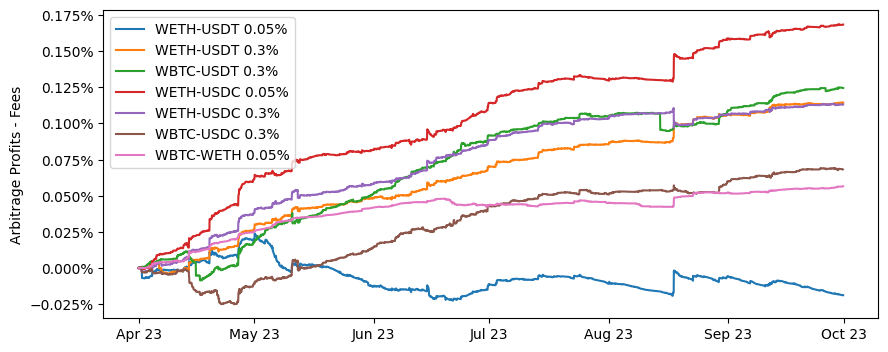
(a) Highly traded pairs between ETH, BTC and stablecoins.

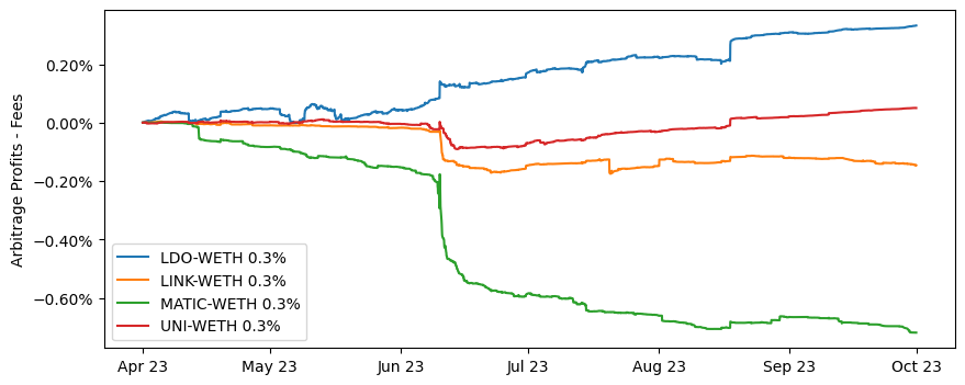
(b) Less traded pairs, with Binance prices obtained by combining the prices of the two respective USDT pairs.

Figure 6: Comparison over six months (April 2023 to October 2023): The difference between the return of providing liquidity to an FM-AMM and on Uniswap v3. Note that, relative to FM-AMM LPs, Uniswap v3 LPs lose to arbitrageurs but gain fees from noise traders. Comparing the return of the two liquidity positions is therefore equivalent to arbitrageurs’ profits minus fees collected from noise traders on Uniswap v3.

Figure 6 shows the difference in cumulative returns between a simulated FM-AMM and the corresponding Uniswap v3 pool. For each trading pair, the FM-AMM trading fee is set equal to the fee of the Uniswap v3 pool we are comparing to.

For most high-volume pairs, providing liquidity on FM-AMM consistently outperforms providing liquidity on Uniswap (see Figure 6(a)). The ETH-USDT 0.05% pool is the only exception, as the FM-AMM and Uniswap v3 returns are approximately equal. Remember that the comparison between FM-AMM and Uniswap v3 illustrates whether trading fees exceed or fall short of arbitrage profits on Uniswap V3. With this respect, our results indicate that providing liquidity to the largest and most traded Uniswap v3 pools is unprofitable: trading fees in these pools do not sufficiently compensate liquidity providers for arbitrage losses. On the other hand, for pools containing less-traded tokens, the results are mixed, with Uniswap v3 outperforming FM-AMM on some token pairs (see Figure 6(b)). However, the absolute difference between cumulative returns is generally quite small. We conjecture that an FM-AMM earning fees from noise traders would have outperformed Uniswap v3 in all cases.

FM-AMM fees

So far, we assumed that the simulated FM-AMM has the same fee as the corresponding Uniswap pool. We now explore whether choosing a different fee would have generated higher returns for FM-AMM LPs.

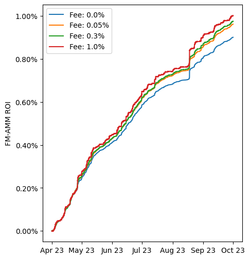
(a) ETH-USDT

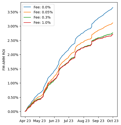
(b) LDO-ETH

Figure 7: Return on providing liquidity to an FM-AMM, for different fees: 0.0%, 0.05%, 0.3%, 1.0%

Remember that the fee affects the size of the rebalancing trade, with higher fees implying smaller rebalancing trades (cf equation 3), which always occur at the new equilibrium price. The fee also determines whether arbitrageurs rebalance the pool, with higher fees implying a lower probability that the pool will be rebalanced. In turn, the probability of rebalancing impacts the return of providing liquidity to FM-AMM because of path dependence. For example, an FM-AMM earns more when it settles one large batch instead of two smaller batches trading in the same direction. In this case, rebalancing less frequently may be beneficial. However, settling a single large batch in which opposite trades net out may generate little or no trade (and hence little or no benefit to the FM-AMM), while settling two smaller batches trading in opposite directions moves the FM-AMM “up the curve” each time. In this case, rebalancing more frequently may be more beneficial.

Figure 7 shows two examples, one in which a fee of zero is optimal and another in which a strictly positive fee is optimal (see Appendix B for additional token pairs). In most cases, the optimal fee is zero, which implies more frequent rebalancing. There are exceptions, though, where LP returns on an FM-AMM would have been highest for a larger-than-zero fee.

Of course, these results do not necessarily extend to an FM-AMM with a positive volume of noise trading. They, however, illustrate that in the previous comparison with Uniswap v3, it is restrictive to use for FM-AMM the same fee as for Uniswap v3. For example, the MATIC-ETH FM-AMM with no noise traders and the same fee as Uniswap v3 underperforms Uniswap v3 by 0.65%, which is reduced to 0.39% if the FM-AMM has zero fee.

6 Discussion: attack model.

In our model, we assumed that batching is an off-chain component of the AMM. Although other implementations are possible (see Section 3.3), it is worth discussing a vulnerability introduced by this assumption: the malicious “batch operator”.

Because the batching process is done off-chain, an entity must collect trades, settle them peer-to-peer whenever possible, and settle the rest on the FM-AMM as a single transaction. We call this entity the “batch operator”. The smart contract managing the FM-AMM can guarantee that the batch operator cannot perform multiple transactions per block on the FM-AMM (hence preventing manipulation by splitting trades as described in Section 3.2). However, the batch operator has full discretion over what transactions are included in the batch and could exploit the FM-AMM by suppressing trades and acting as the “unique arbitrageur.” Similarly to the first arbitrageur reaching a CFAMM after a change in the equilibrium price, the batch operator is the only entity that can rebalance the pool and will exploit this opportunity to maximize profits.

More precisely, suppose the external price is $p^{*}$ and that the liquidity reserves on the FM-AMM are $X$ and $Y$ (in ETH and DAI, respectively). The malicious batch operator trades $x$ so to maximize its profits:

$$\max_{x}\left\{x\cdot p^{*}-x\cdot\frac{Y}{X-2\cdot x}\right\}=\frac{Y+p^{*}X}{2}-\sqrt{XYp^{*}}.$$

Compare this to the profits earned by an arbitrageur rebalancing a CPAMM also with reserves $X$ and $Y$, which are

$$\max_{x}\left\{x\cdot p^{*}-x\cdot\frac{Y}{X-x}\right\}=Y+p^{*}X-2\sqrt{XYp^{*}}.$$

Note that arbitrageurs’ and batch operators’ profits are at the expense of their respective LPs. The above derivations, therefore, show that the loss that FM-AMM’s LPs may face from a malicious batch operator are half of the losses that CPAMM’s LPs routinely face from arbitrageurs.

To conclude, note that the batch operator’s behavior is observable ex-post on-chain. It is, therefore, possible to introduce punishments on the batch operator in case it misbehaves. There could be social punishments such as LPs withdrawing their liquidity (and hence making FM-AMM useless), automated slashing of dedicated funds, or even legal remedies if the batch operator is a legal entity.

7 Conclusion

This paper studies the design of AMM when trades are batched before reaching the AMM. The key observation is that, because of batching, the AMM does not need to satisfy path independence, which implies that the design space is larger than without batching. In particular, it is possible to design a function maximizing AMM (FM-AMM), which, for given prices, always trades to be on the highest possible value of a given function. At the same time, batching creates competition between informed arbitrageurs. As a result of this competition, the price at which the FM-AMM trades is always equal to the equilibrium price (assumed determined on some very liquid location and exogenous to the FM-AMM). Hence, whereas in a traditional CFAMM, arbitrageurs earn profits at the expense of liquidity providers, in an FM-AMM these profits remain with its LPs. At the same time, sandwich attacks are eliminated because all trades within the same batch occur at the same price, equal to the exogenously determined equilibrium price. We use Binance price data for 11 token pairs over a period of six months to simulate a lower bound to the return of providing liquidity to an FM-AMM. We find that this lower bound generally outperforms providing the same liquidity on Uniswap v3, and that the absolute differences between the two are small.

Our results are robust to several extensions. In particular, in the companion paper Canidio and Fritsch (2023), we study the case in which the batch operator can settle the trades on the batch both on the FM-AMM and also on some other CFAMM (while the FM-AMM can only be accessed via the batch). Also in that version of the model, competition among arbitrageurs guarantees that the FM-AMM always trades at the equilibrium price. The only difference is that arbitrageurs may rebalance the FM-AMM and the CFAMM by trading with the batch and then simultaneously backrunning the batch on the CFAMM. In that case, arbitrageurs earn strictly positive profits at the expense of the CFAMM liquidity providers.

As discussed in the introduction, by eliminating sandwich attacks and arbitrage profits, an FM-AMM also eliminates the vast majority of MEV. If it were widely adopted, the only remaining MEV source of measurable size would be liquidation in the context of lending protocols. In blockchain-based lending protocols, users borrow a given token by pledging a different token as collateral. The collateral is liquidated when its value drops below a threshold: the protocol sells it to whoever pays the liquidation price—usually well below its market value—and returns the borrowed amount. This naturally creates competition between liquidation bots and, therefore, MEV. We conjecture that if the liquidation process were forced through the FM-AMM batch, the liquidation would occur at the fair equilibrium price, eliminating this remaining source of MEV. Fully exploring this possibility is left for future work.

Appendix A Mathematical derivations

Proof of Proposition 2.

Suppose nose traders collectively submit trade $a(i)>0$ (the case $a(i)<0$ is analogous). If arbitrageurs also submit a trade $r(i)>0$, then by (5) the effective price they pay is $\frac{Y}{(1-\tau)(X-2(a(i)+r(i)))}$. If instead they submit $r(i)<0$ with $a(i)+r(i)\leq 0$, then the effective price they pay is $\frac{Y(1-\tau)}{X-2(1-\tau)(a(i)+r(i))}$. If instead they submit $r(i)<0$ with $a(i)+r(i)\geq 0$, then the effective price they pay is $\frac{Y(1-\tau)}{X-2(a(i)+r(i))}$. The price faced by arbitrageurs as a function of their trade is therefore discontinuous at $r(i)=0$, where arbitrageurs shift from paying the buy price $\frac{Y}{(1-\tau)(X-2a(i))}$ to paying the sell price $\frac{Y(1-\tau)}{X-2a(i)}$. For $r(i)\neq 0$, instead, the effective price paid by the arbitrageurs is continuous, strictly increasing, goes to zero for $r(i)\rightarrow-\infty$ and to infinity for $r(i)\rightarrow X-a(i)$.

Hence, if $p^{*}(\mu\cdot i-\gamma)>\frac{Y}{(1-\tau)(X-2a(i))}$ or $p^{*}(\mu\cdot i-\gamma)<\frac{Y(1-\tau)}{X-2a(i)}$, then there exists a unique $r^{*}(i)$ such that

$$\tilde{p}(a(i)+r^{*}(i),r^{*}(i),\tau)=p^{*}(\mu\cdot i-\gamma),$$

In this case, $r^{*}(i)$ is an equilibrium because no arbitrageur can be better off by trading more or less with the batch. The fact that such an equilibrium is unique can be established by contradiction: suppose the equilibrium is $r^{\prime}$ with $\tilde{p}(a(i)+r^{\prime},r^{\prime},\tau)\neq p^{*}(k\cdot i-\gamma)$. Then by the fact that $\tilde{p}(a(i)+r^{\prime},r^{\prime}\tau)$ is locally continuous in $r^{\prime}$, an arbitrageur could submit an additional trade $k$ such that $\tilde{p}(a(i)+r^{\prime}+k,r^{\prime}+k,\tau)\neq p^{*}(k\cdot i-\gamma)$ and earn strictly positive profits, which implies that $r^{\prime}$ is not an equilibrium.

Finally, it is easy to check that if $p^{*}(k\cdot i-\gamma)\in[\frac{Y}{(1-\tau)(X-2a(i))},\frac{(1-\tau)Y}{X-2a(i)}]$, then arbitrageurs have no profitable trade opportunity: if arbitrageurs also buy ETH they pay at least $\frac{(1-\tau)Y}{X-2a(i)}$, which is greater than the equilibrium price; if arbitrageurs sell ETH they receive at most $\frac{Y}{(1-\tau)(X-2a(i))}$ per ETH sold, which is less than the equilibrium price.

∎

Proof of Proposition 3.

Note that the volume of noise trading is independent of the price. Hence, for given prices, a FM-AMM maximizes $V(p,\tau)=\max_{x}U(x+a(i),p,\tau)$ with demand function (net of noise trading) given by $x(p,\tau)\equiv\mbox{argmax}_{x}U(x+a(i),p,\tau)\neq 0$.

The first observation is that the value function $V(p,\tau)=\max_{x}U(x+a(i),p,\tau)$ is convex in $p$, strictly so if there is strictly positive trade (i.e., if $x(p,\tau)\neq 0$). To see this, use the envelope theorem to write:

$$\frac{\partial V(p,\tau)}{\partial p}=\begin{cases}\left(X-x(p,\tau)-a(i)\right)x(p,\tau)&\mbox{ if }x(p,\tau)>0\\ \left(\frac{X}{1-\tau}-x(p,\tau)-a(i)\right)x(p,\tau)&\mbox{ if }x(p,\tau)<0\\ 0&\mbox{ if }x(p,\tau)=0\end{cases}$$

so that

$$\frac{\partial^{2}V(p,\tau)}{\partial p^{2}}=\begin{cases}\frac{\partial x(p,\tau)}{\partial p}\left(X-a(i)-2x(p,\tau)\right)&\mbox{ if }x(p,\tau)>0\\ \frac{\partial x(p,\tau)}{\partial p}\left(\frac{X}{1-\tau}-a(i)-2x(p,\tau)\right)&\mbox{ if }x(p,\tau)<0\\ 0&\mbox{ if }x(p,\tau)=0\end{cases}$$

Because $p$ and $x$ are strict complements in the objective function, by Topkis’s theorem, $\frac{\partial x(p,\tau)}{\partial p}>0$ whenever $x(p,\tau)\neq 0$. Also, the FM-AMM always trades so that $\left(X-a(i)-2x(p,\tau)\right)>0$ and $\left(\frac{X}{1-\tau}-a(i)-2x(p,\tau)\right)>0$. It follows that $V(p,\tau)$ is strictly convex in $p$ whenever $x(p,\tau)\neq 0$.

Next, note that if there is a rebalancing event, then $p=p^{*}(\mu\cdot i-\gamma)$. If there is no rebalancing event, then $V(p,\tau)$ is independent of the price. Because $F()$ is a mean-preserving spread of $G()$, then

$$E_{F}[V(p,\tau)]\geq E_{G}[V(p,\tau)]$$

with strict inequality as long as $x(p,\tau)>0$ (i.e., there is a rebalancing event) for some realization of $p^{*}(\mu\cdot i-\gamma)$. ∎

Appendix B Extra figures

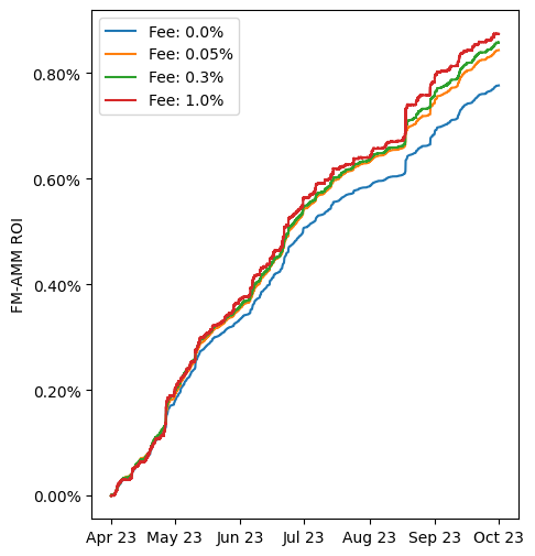
(a) BTC-USDT

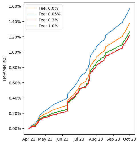
(b) LINK-ETH

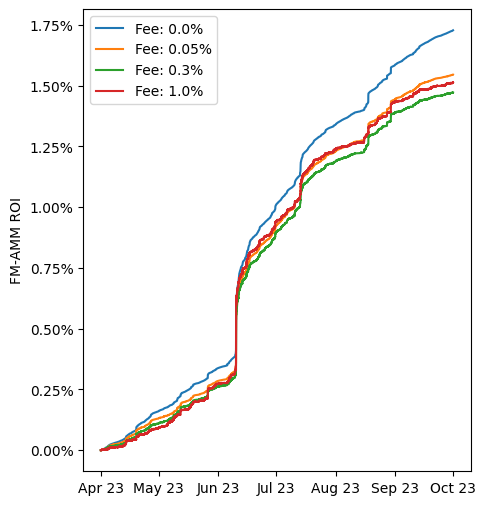
(c) MATIC-ETH

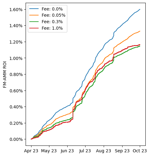
(d) UNI-ETH

Figure 8: Return on providing liquidity to an FM-AMM, for different fees: 0.0%, 0.05%, 0.3%, 1.0%

References

- Aoyagi (2020) Aoyagi, J. (2020). Liquidity provision by automated market makers. working paper.
- Breidenbach et al. (2018) Breidenbach, L., P. Daian, F. Tramèr, and A. Juels (2018). Enter the hydra: Towards principled bug bounties and Exploit-Resistant smart contracts. In 27th USENIX Security Symposium (USENIX Security 18), pp. 1335–1352.
- Budish et al. (2015) Budish, E., P. Cramton, and J. Shim (2015). The high-frequency trading arms race: Frequent batch auctions as a market design response. The Quarterly Journal of Economics 130(4), 1547–1621.
- Canidio and Danos (ming) Canidio, A. and V. Danos (forthcoming). Commitment against front-running attacks. Management Science.
- Canidio and Fritsch (2023) Canidio, A. and R. Fritsch (2023). Batching Trades on Automated Market Makers. In J. Bonneau and S. M. Weinberg (Eds.), 5th Conference on Advances in Financial Technologies (AFT 2023), Volume 282 of Leibniz International Proceedings in Informatics (LIPIcs), Dagstuhl, Germany, pp. 24:1–24:17. Schloss Dagstuhl – Leibniz-Zentrum für Informatik.
- Capponi and Jia (2021) Capponi, A. and R. Jia (2021). The adoption of blockchain-based decentralized exchanges. arXiv preprint arXiv:2103.08842.
- Chainlink (2020) Chainlink (2020). What is the blockchain oracle problem? Retrieved from https://chain.link/education-hub/oracle-problem on May 24, 2023. Online forum post.
- Della Penna (2022) Della Penna, N. (2022, September 1). Mev minimizing amm (minmev amm). Retrieved from https://ethresear.ch/t/mev-minimizing-amm-minmev-amm/13775 on May 24, 2023. Online forum post.
- Ferreira and Parkes (2023) Ferreira, M. V. X. and D. C. Parkes (2023). Credible decentralized exchange design via verifiable sequencing rules.
- Foley et al. (2022) Foley, S., P. O’Neill, and T. Putnins (2022). Can markets be fully automated? evidence from an automated market maker. Technical report, Working Paper, Macquarie University.
- Gans and Holden (2022) Gans, J. S. and R. T. Holden (2022). A solomonic solution to ownership disputes: An application to blockchain front-running. Technical report, National Bureau of Economic Research.
- Heimbach et al. (2023) Heimbach, L., L. Kiffer, C. Ferreira Torres, and R. Wattenhofer (2023). Ethereum’s proposer-builder separation: Promises and realities. In Proceedings of the 2023 ACM on Internet Measurement Conference, pp. 406–420.
- Heimbach et al. (2024) Heimbach, L., V. Pahari, and E. Schertenleib (2024). Non-atomic arbitrage in decentralized finance. arXiv preprint arXiv:2401.01622.
- Heimbach et al. (2022) Heimbach, L., E. Schertenleib, and R. Wattenhofer (2022). Risks and returns of uniswap v3 liquidity providers. arXiv preprint arXiv:2205.08904.
- Heimbach et al. (2021) Heimbach, L., Y. Wang, and R. Wattenhofer (2021). Behavior of liquidity providers in decentralized exchanges.
- Johnson et al. (2023) Johnson, N. A., T. Diamandis, A. Evans, H. de Valence, and G. Angeris (2023). Concave pro-rata games. arXiv preprint arXiv:2302.02126.
- Josojo (2022) Josojo (2022, August 4). Mev capturing amm (mcamm). Retrieved from https://ethresear.ch/t/mev-capturing-amm-mcamm/13336 on May 24, 2023. Online forum post.
- Lehar and Parlour (2021) Lehar, A. and C. A. Parlour (2021). Decentralized exchanges. working paper.
- Leupold (2022) Leupold, F. (2022, November 1). Cow native amms (aka surplus capturing amms with single price clearing). Retrieved from https://forum.cow.fi/t/cow-native-amms-aka-surplus-capturing-amms-with-single-price-clearing/1219/1 on May 24, 2023. Online forum post.
- Loesch et al. (2021) Loesch, S., N. Hindman, M. B. Richardson, and N. Welch (2021). Impermanent loss in uniswap v3.
- Malinova and Park (2023) Malinova, K. and A. Park (2023). Learning from defi: Would automated market makers improve equity trading?
- Milionis et al. (2023) Milionis, J., C. C. Moallemi, and T. Roughgarden (2023). Automated market making and arbitrage profits in the presence of fees. arXiv preprint arXiv:2305.14604.
- Milionis et al. (2022) Milionis, J., C. C. Moallemi, T. Roughgarden, and A. L. Zhang (2022). Automated market making and loss-versus-rebalancing. arXiv preprint arXiv:2208.06046.
- Park (2023) Park, A. (2023). The conceptual flaws of decentralized automated market making. Management Science 69(11), 6731–6751.
- Qin et al. (2022) Qin, K., L. Zhou, and A. Gervais (2022). Quantifying blockchain extractable value: How dark is the forest? In 2022 IEEE Symposium on Security and Privacy (SP), pp. 198–214. IEEE.
- Ramseyer et al. (2023) Ramseyer, G., M. Goyal, A. Goel, and D. Mazières (2023). Augmenting batch exchanges with constant function market makers. arXiv preprint arXiv:2210.04929.
- Schlegel and Mamageishvili (2022) Schlegel, J. C. and A. Mamageishvili (2022). Axioms for constant function amms. arXiv preprint arXiv:2210.00048.
- Torres et al. (2021) Torres, C. F., R. Camino, et al. (2021). Frontrunner jones and the raiders of the dark forest: An empirical study of frontrunning on the ethereum blockchain. In 30th USENIX Security Symposium (USENIX Security 21), pp. 1343–1359.