XX \jnumXX \paper8 \jmonthMay/June
Department: Head \editorEditor: Name, xxxx@email
Performance Modeling of Data Storage Systems using Generative Models
Abstract
High-precision modeling of systems is one of the main areas of industrial data analysis. Models of systems, their digital twins, are used to predict their behavior under various conditions. We have developed several models of a storage system using machine learning-based generative models. The system consists of several components: hard disk drive (HDD) and solid-state drive (SSD) storage pools with different RAID schemes and cache. Each storage component is represented by a probabilistic model that describes the probability distribution of the component performance in terms of IOPS and latency, depending on their configuration and external data load parameters. The results of the experiments demonstrate the errors of 4–10 % for IOPS and 3–16 % for latency predictions depending on the components and models of the system. The predictions show up to 0.99 Pearson correlation with Little’s law, which can be used for unsupervised reliability checks of the models. In addition, we present novel data sets that can be used for benchmarking regression algorithms, conditional generative models, and uncertainty estimation methods in machine learning.
Introduction Data storage systems (DSS) are of vital importance in the modern world. The emergence of big data has necessitated the development of storage systems with a larger capacity and lower costs to efficiently store and process the vast amounts of data generated [1, 2]. Performance modeling is essential in the development of such systems. The modeling allows engineers to analyze the system’s behavior under different conditions and helps them to find the optimal design of the system. It can be used for marketing purposes to estimate the system performance under the customer’s requirements. One more application is diagnostics and predictive maintenance, where model predictions are compared with actual measurements to detect failures and anomalies.
The key components of a typical DSS are controllers, fast cache memory, and storage pools. All data are stored in the pools consisting of several hard disk drives (HDDs) or solid-state drives (SSDs) united with raid schemes. The cache speeds up read and write operations with the most popular data blocks. And the controllers are responsible for data management and provide computational resources to process all input and output requests from users.
An early attempt to model SSDs was described in [3]. The authors argue that HDD performance models cannot be used for SSD due to certain unique SSD characteristics, such as low latency, slow update, and expensive block-level erasure. The black-box approach to model SSD performance is suggested as it requires minimal a priori information about the device. The researchers found that although black-box simulation does not produce high-quality predictions for HDDs, it can produce accurate ones for SSDs.
Another paper presents a black-box approach based on regression trees to model performance metrics for SSDs [4]. The resulting model can accurately predict latency, bandwidth, and throughput with mean relative errors of 20 %, 13 %, and 6 %, respectively.
The authors of paper [5] propose SSDcheck, a novel SSD performance model, which is capable of extracting various internal mechanisms and predicting the latency of the next access to commodity SSDs. SSDcheck can dynamically manage the model to accurately predict latency and extract useful internal mechanisms to fully exploit SSDs. Additionally, the paper presents multiple practical cases evaluated to show significant performance improvement in various scenarios. The proposed use cases also leverage the performance model and other features to achieve an improvement of up to 130 % in overall throughput compared to the baseline.
Machine learning techniques have proved to be useful in the task of analyzing the disks. As an example, the main approaches discussed in [6] are based on machine learning. The paper uses a methodology that extracts low-cost history-aware features to train SSD performance models which predict response times to requests. The paper also utilizes space-efficient data structures such as exponentially decaying counters to track past activity with memory and processing cost. Lastly, the paper uses machine learning models such as decision trees, ensemble methods, and feedforward neural networks to predict the storage hardware response time. All of these approaches are designed to make accurate SSD simulators more accessible and easier to use in real-world online scenarios.
The authors of paper [7] developed an open-source disk simulator called IMRSim to evaluate the performance of two different allocation strategies for interlaced magnetic recording (IMR) technology using a simulation designed in the Linux kernel space using the Device Mapper framework and offers a scalable interface for interaction and visualization of input and output (I/O) requests.
Another open-source simulator was developed in [8]. The authors introduce SimpleSSD, a high-fidelity holistic SSD simulator. Aside from modeling a complete storage stack, this simulator decouples SSD parallelism from other flash firmware modules, which helps to achieve a better simulation structure. SimpleSSD processes I/O requests through layers of a flash memory controller. The requests are then serviced by the parallelism allocation layer, which abstracts the physical layout of interconnection buses and flash disks. While being aware of internal parallelism and intrinsic flash latency, the simulator can capture close interactions among the firmware, controller, and architecture.
The idea of SimpleSSD has been further developed in [9]. SimpleSSD 2.0, namely Amber, was introduced to run in a full system environment. Being an SSD simulation framework, Amber models embedded CPU cores, DRAMs, and various flash technologies by emulating data transfers. Amber applies parallelism-aware readahead and partial data update schemes to mimic the characteristics of real disks.
Research that used different Flash Translation Layer (FTL) schemes was presented in [10]. FlashSim, an SSD simulator, has been developed to evaluate the performance of storage systems. The authors analyzed the energy consumption in different FTL schemes to find realistic workload traces and validated FlashSim against real commercial SSDs and detected behavioral similarities.
Although simulating SSD devices might have seemed an exciting research topic, older kinds of storage system has also received the scientific attention it deserves. One of the papers presents a series of HDD simulations to investigate the stiffness of the interface between the head and the disk. In [11], the authors develop a finite-element model of an HDD using a commercially available three-dimensional modeling package. The results of the numerical analysis gave insights into the characteristics of each type of shock applied to an HDD model.
Although used extensively in modern times, SSDs are not designed perfectly. There is a certain performance-durability trade-off in their design. Disks of this type require garbage collection (GC), which hinders I/O performance, while the SSD block can only be erased a finite number of times. There is research that proposes an analytical model that optimizes any GC algorithm [12]. The authors propose the randomized greedy algorithm, a novel GC algorithm, which can effectively balance the above-mentioned trade-off.
In the search for the perfect architecture of a modern SSD through design space exploration (DSE), researchers have come across the challenge of fast and accurate performance estimation. In [13], the authors suggest two ways to tackle this challenge: scheduling the task graph and estimation based on neural networks (NN). The proposed NN regression model is based on training data, which consists of hardware configurations and performance. The paper concludes that the NN-based method is faster than scheduling-based estimation and is preferred for scalable DSE.
The evaluation of SSD performance has also been investigated in [14]. SSDs are built using an integrated circuit as memory, so manufacturers are interested in I/O traces of applications running on their disks. This paper proposes a framework for the accurate estimation of I/O trace execution time on SSDs.
All of these solutions have a range of limitations. The first one is that they are focused mostly on the modeling of one single device such as HDD or SSD disks. The second is that most of them are based on the simulation of physical processes and the firmware stack inside the devices which require more resources for development. But one of the main disadvantages is that the models do not take into account vendor specifics of the devices due to the trade secrets. In result, errors of the performance simulation are quite high for practical use. Finally, HDDs and SSDs are part of DSS with unique architectures and software that influence the device performance and are not taken into account in the solutions described above.
In this work, we present a data-driven approach for DSS modeling which does not have these limitations. All vendor specifics, architecture features, and software impact are learned directly from real performance measurements of the system. We present the performance modeling and analysis of a data storage cache, SSD, and HDD pools under random and sequential data loads. We provide novel data sets of IOPS and latency measurements for the system’s components for various configurations and load parameters. We consider two different approaches to learn distributions of the performance values, based on parametric and nonparametric generative models. We analyze the quality of the model’s predictions and compare them with a naive baseline algorithm. We also demonstrate a physics-inspired method for checking the reliability of the model predictions. The data sets provided in this work can be used for benchmarking regression algorithms, conditional generative models, and uncertainty estimation methods in machine learning.
Problem statement
| Model | Inputs | Outputs |
|---|---|---|
| Storage pool | Load type, IO type, read fraction, block size, number of jobs, queue depth, number of disks, number of data, and parity blocks in RAID | IOPS, Latency |
| Storage cache | Load type, IO type, read fraction, block size, number of jobs, queue depth | IOPS, Latency |
In this study, we consider the simulation of HDD and SSD storage pools, and cache, which are the key parts of data storage systems. The goal of this work is to predict the performance of these components for a given configuration and data load parameters. We describe the performance by the number of input and output operations per second (IOPS) and the average of their latencies. The data load is parameterized by: load type, IO type, read fraction, block size, number of jobs, and queue depth for each of these jobs. There are two load types we consider in the work: random and sequential. Each data load consists of a mixture of read and write operations. The IO type indicates whether we consider read or write operations in our simulations. The read fraction is the ratio of the number of read operations to the total number of all operations in the data load. Each operation processes one data block of a given size. And the data loads are generated by several jobs with a given queue depth.
HDD and SSD storage pools also have configuration parameters. They are the total number of disks in a pool and the RAID scheme, which is described by the number of data and parity blocks. In this work, the cache has only one configuration, and we do not describe it by any parameter. The lists of input and output features in our simulation models are shown in Table 1.
Let us denote the vector of input features as , and the vector of outputs as . Also suppose we have pairs of measurements of output vectors for the given inputs . These pairs are obtained by generating various data loads on a real data storage system and measuring the performances of its pool or cache in terms of IOPS and latency. The goal of this work is to estimate the conditional probability distribution for the storage component using machine learning. Then, we predict the performance for the unknown inputs by sampling from the learned distribution:
| (1) |
The advantage of this data-driven approach is that we do not need to understand and simulate all the physical processes inside the storage components. The model only needs a sample of measurements. Machine learning algorithms estimate all physical dependencies from the data. We can use this model to explore and visualize the performance dependencies from the configuration and data load parameters, to predict the average performance and its deviations for new conditions, and to analyze many other properties.
Data collection
| Parameter | Value range |
|---|---|
| Load type | random |
| Block size | 4, 8, 16, 32, 64, 128, 256 KB |
| Read fraction | 0 - 100% |
| Number of jobs | 1 - 64 |
| Queue depth | 1 - 16 |
| Parameter | Value range |
|---|---|
| Load type | random |
| Block size | 4, 8, 16, 32, 64 KB |
| Read fraction | 0 - 100% |
| Number of jobs | 1 - 32 |
| Queue depth | 1 - 32 |
| RAID (K+M) | 1+1, 2+1, 2+2, 4+1, 4+2, 8+2 |
| Number of disks | K+2M, 24, +3 values in between |
| Parameter | Value range |
|---|---|
| Load type | sequential |
| Block size | 128, 256, 512, 1024 KB |
| Read fraction | 0% |
| Number of jobs | 1 - 20 |
| Queue depth | 1 - 32 |
| RAID (K+M) | 1+1, 2+1, 2+2, 4+1, 4+2, 8+2 |
| Number of disks | K+2M, 24, +3 values in between |
| Parameter | Value range |
|---|---|
| Load type | sequential |
| Block size | 128, 256, 512, 1024 KB |
| Read fraction | 0, 100% |
| Number of jobs | 1 - 20 |
| Queue depth | 1 - 32 |
| RAID (K+M) | 1+1, 2+1, 2+2, 4+1, 4+2, 8+2 |
| Number of disks | K+2M, 24, +3 values in between |
For this study, we collected four data sets for the storage pools and cache under different data loads. The first one is for the cache under the random data loads. To collect it, we generated 510 different data loads using a performance analysis tool Perf [15] in Linux. Table 2 provides the list of the load parameters and the ranges of their values. We quasi-randomly selected these values for each individual data load using the Sobol sequence [16]. This method covers the parameter space more uniformly than random or grid sampling. Each load lasted 60 seconds, and for every second we measured IOPS and average latency for read and write operations separately. In the results, we collected pairs of measurements .
Similarly, we collected data sets for the SSD pool under random loads. The list of all parameters and their value ranges is in Table 3. In this case, we also used the pool configuration parameters in addition to the data load ones. The first is a RAID scheme, which is defined by the number of data (K) and parity (M) blocks. The second is the total number of disks in the pool. We generated 512 different loads in total for various pool configurations with a duration of 120 seconds each. We measured IOPS and average latency for read and write operations separately every second. In the results, this data set contains pairs of measurements .
We also collected two data sets for SSD and HDD storage pools under sequential data loads. We used the same procedure described above. The main difference is that only pure loads with read fractions of 0 and 100 % are valuable. One more difference is that larger block sizes are used for the sequential loads. Table 4 and Table 5 show the full list of the data load and configuration parameters and their value ranges. We used the Sobol sequence to generate 512 different loads in total for various pool configurations with a duration of 120 seconds each. We measured IOPS and average latency for read and write operations every second. In the results, each data set contains pairs of measurements .
Models
CatBoost model
The first model we use in this study is a parametric generative model based on the CatBoost [17] regression model. Relations between IOPS and latencies within the same data load are defined by Little’s law [18]:
| (2) |
where is the queue depth and is the number of jobs. While the fraction of read operations is fixed during each data load, Little’s law allows us to suppose the following relation for read or write operations:
| (3) |
All measurements of IOPS and latencies are stochastic. We approximate the distribution of their logarithm values by conditional 2D normal distributions:
| (4) |
| (5) |
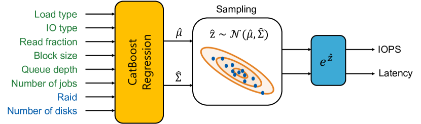
where is a vector of predictions for IOPS and latency; the mean and the covariance matrix depend on input vector of data load and configuration parameters, and are predicted by the CatBoost regression model. Figure 1 shows the model.
As described in the previous section, a sample contains read and write data loads with measurements in each for just read or write operations. The total number of measurements is . We calculate the mean vectors and the covariance matrices for each of these data loads. In addition, we use Cholesky decomposition [19] for the matrices . It is used to ensure that the predicted covariance matrices will be positive semi-definite. We fit the CatBoost regression model with the MutliRMSE loss function defined as:
| (6) |
where . The model consists of 5000 decision trees. The optimal hyperparameters values of the CatBoost regressor are estimated using a grid search for each storage system component.
Normalizing flow
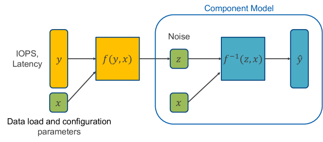
The second model we apply in this work is based on Normalizing Flows (NF) [20]. Consider a sample with measurements for various data loads and configurations of a data storage component. Let us also define a latent random variable with the standard normal distribution . The goal of the NF model is to learn an invertible transformation between the vector of measured IOPS and latency into the latent variable with the given :
| (7) |
The change of variable theorem determines the relation between the estimated performance and the latent variable distributions:
| (8) |
In this work, we use the real-valued non-volume preserving (Real NVP) NF model [21], where the function is designed using a chain of neural networks. The model is fitted by maximizing the log-likelihood function:
| (9) |
Predictions of the performance values are performed as , where is a randomly sampled vector from the distribution. An illustration of the NF model is shown in Figure 2. In this case, is sampled from the learned distribution of the IOPS and latency with the given data load and configuration parameter values.
In our experiments, we use sixteen Real NVP transformations, where two simple 2-layer fully connected neural networks are exploited in each transformation. The model uses the Adam optimizer and the tanh activation function. It trains for 80 epochs with a batch size of 200 and a learning rate
kNN model
Consider a new vector of inputs for which we need to predict IOPS and latency values. As previously, assume that our train sample contains read and write data loads with measurements in each. The total number of observations is . All these data loads are described by unique input vectors . Then, for the new input the k Nearest Neighbours (kNN) algorithm searches for the nearest vector :
| (10) |
where is the distance between two input vectors. In this work, we used the Euclidean distance. The predictions are performed as follows. The model takes for the predictions all observations for which :
| (11) |
In other words, the model finds the closest known data load to the new one and takes its measured IOPS and latencies as predictions. We use this approach as a baseline in the study. This helps to estimate whether the CatBoost and the NF models based on machine learning algorithms provide better prediction results than the naive approach based on the kNN algorithm.
Quality metrics
Consider the measurements for just read or write operations in one single data load. According to the data sets description, this sample contains 120 (60 for cache) measurements, where all have the same input feature values, and is a vector of measured performance values. Also, suppose that we have predictions from one of the models for the same . The goal is to estimate the discrepancy between the distributions of and .
The first quality metric we use is the Percentage Error of Mean (PEM), which describes the ability of the models to predict mean values of IOPS and latency for each data load:
| (12) |
| (13) |
Similarly, we use the Percentage Error of Standard deviation (PES), which describes the ability of the models to predict standard deviations of IOPS and latency values for each data load:
| (14) |
| (15) |
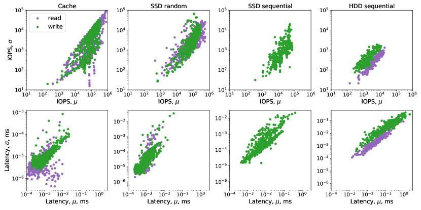
The means () and standard deviations () of the measured IOPS and latencies for cache, SSD, and HDD pools under random and sequential data loads are shown in Figure 3.
We also use two additional metrics to measure the distances between the distributions of and . The first is the Fréchet distance (FD) [22], which is widely used to estimate the quality of generative models [23]. We suppose that the vectors and have 2D Gaussian distributions and respectively. Then, the FD is defined as:
| (16) |
One more metric is the Maximum Mean Discrepancy (MMD) [24], which is defined as:
| (17) |
where is the Radial Basis Function (RBF) with normalization constant and equals the median distance between the vectors in the combined sample and .
In our study, IOPS and latency have different scales which affect the calculation of the FD and MMD. To solve this problem, we fit the Standard Scaler [25] on the real observations and apply it to transform the values of and . Then, the scaled vectors are used for the FD and MMD estimation.
We split data loads in each data set into train and test samples. Test one contains 100 random data loads with all their measurements . For each model, we calculate the quality metrics on each individual data load. Then, we use the bootstrap technique to find their average and standard deviation over all loads in the test sample.
Results
| Metric | kNN | CatBoost | NF |
|---|---|---|---|
| PEM (IOPS), % | 262 | 6.30.4 | 4.10.4 |
| PEM (Lat), % | 181 | 4.90.3 | 2.90.2 |
| PES (IOPS), % | 352 | 23.90.8 | 41223 |
| PES (Lat), % | 301 | 24.10.9 | 29929 |
| FD | 6655822 | 44557 | 36555 |
| MMD | 1.610.01 | 1.340.02 | 0.590.02 |
| Metric | kNN | CatBoost | NF |
|---|---|---|---|
| PEM (IOPS), % | 383 | 8.90.6 | 10.10.8 |
| PEM (Lat), % | 19.20.9 | 7.40.4 | 8.80.6 |
| PES (IOPS), % | 523 | 220.9 | 18314 |
| PES (Lat), % | 402 | 251.1 | 1359 |
| FD | 1647211 | 14019 | 16116 |
| MMD | 1.380.02 | 1.050.02 | 0.830.02 |
| Metric | kNN | CatBoost | NF |
|---|---|---|---|
| PEM (IOPS), % | 313 | 10.20.9 | 9.91 |
| PEM (Lat), % | 423 | 10.70.7 | 8.10.7 |
| PES (IOPS), % | 9012 | 375 | 13416 |
| PES (Lat), % | 10116 | 425 | 13117 |
| FD | 1692241 | 11018 | 8919 |
| MMD | 1.230.03 | 1.010.03 | 0.690.03 |
| Metric | kNN | CatBoost | NF |
|---|---|---|---|
| PEM (IOPS), % | 272 | 10.60.9 | 11.40.9 |
| PEM (Lat), % | 494 | 162 | 182 |
| PES (IOPS), % | 333 | 181 | 434 |
| PES (Lat), % | 608 | 232 | 627 |
| FD | 9619 | 5.00.6 | 6.70.9 |
| MMD | 0.810.04 | 0.330.02 | 0.230.02 |
In this section, we consider the experiments we have conducted to estimate the quality of the models111https://github.com/HSE-LAMBDA/digital-twin. We fitted all models described above on the same train samples, made predictions on the same test samples, and calculated quality metrics from the previous section. The metrics values for the cache, SSD, and HDD pools are presented in Tables 6, 7, 8, and 9. The models in our study learn the conditional distributions of IOPS and latency. Their predictions are samples from these distributions. Each metric highlights different quality aspects of the prediction, which we detail below.
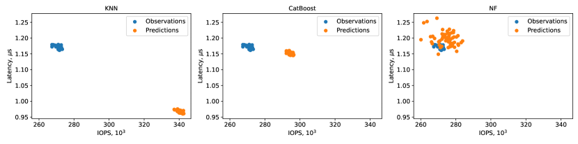
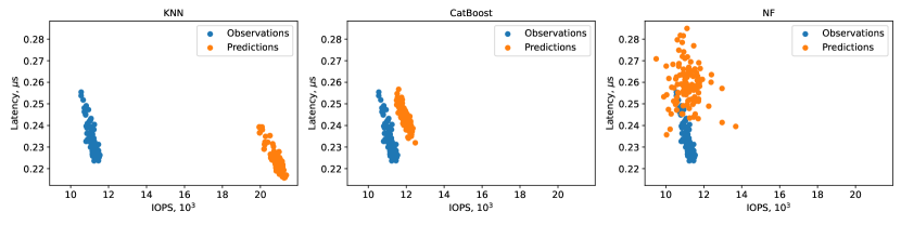
Table 6 provides the metrics values for the kNN, CatBoost, and NF models for the cache under random data loads. Figure 4 shows an example of the predictions for a data load from the test sample. The PEM and PES metrics in the table show the estimation quality of the means and standard deviations, respectively, for IOPS and latency in each data load. The observed means and standard deviations are presented in Figure 3. The NF model demonstrates the best PEM values, where the prediction errors are about 4.1 % and 2.9 % for IOPS and latency, respectively. It is about 6 times smaller than the 25 % and 17.8 % errors for the kNN model. Similarly, CatBoost demonstrates the smallest PES values of 23.9 % and 24.1 % for IOPS and latency, respectively. The NF model has the most significant errors of 412 % and 299 % for IOPS and latency. Generally, the results show that the standard deviation estimation is a challenging task for all models in our study. But the NF predicts the widest distributions, as demonstrated in Figure 4.
FD compares the mean values and the covariance matrices of the predictions and real observations. The metric value for the CatBoost and NF is approximately 15 and 18 times smaller than for the kNN, respectively but still quite large. This can be explained by the following two reasons. The first is the standard scaling transformation that we applied before the metric calculation. It was fitted on real observations and applied to the predictions as we described in the previous section. FD estimates the distance between two distributions on a scale, where the observed IOPS and latencies have zero means and standard deviations of 1. The second reason is that the cache is the fastest component in the data storage system. The standard deviations of its IOPS and latency measurements are relatively small compared to the mean values for other components of the system, as shown in Figure 3. So, the calculated distances between the observed and predicted distributions are larger for the cache than for other components. The MMD metric compares two distributions by calculating distances between pairs of points. The distances are divided by the median values, which makes the metric more robust to different scales of the distributions. The results show that the NF model has the best MMD value.
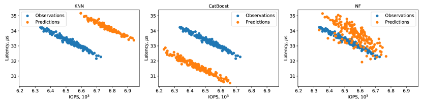
Table 7 presents the metrics values for the kNN, CatBoost, and NF models for the SSD pool of the system under random data loads. Figure 5 shows an example of the predictions for a data load from the test sample. The results demonstrate that the CatBoost model is the best in terms of the FD, PEM, and PES metrics, and NF is the best in terms of the MMD metric. The CatBoost model predicts the mean of IOPS and latency values with errors of 8.9 % and 7.4 % respectively, compared with 38 % and 19.2 % for the kNN. The standard deviations of IOPS and latency are estimated with errors of 22 % and 25 % for CatBoost and 52 % and 40 % for the kNN model. Similarly to the cache, the NF model predicts wider distributions for SSD pools under random data loads as it is reflected in PES values. However, the model estimates the IOPS and latency distributions better in terms of the MMD metric. We explain this behavior as follows. NF learns wider distributions than other models. Despite these distributions having worse PES values, they cover the observations better than other models.
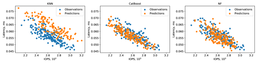
Similarly, Table 8 shows the metrics values for the SSD pool under sequential data loads. Figure 6 shows an example of the predictions for a data load from the test sample. The results demonstrate that the CatBoost model is the best in terms of the FD, and PES metrics, and the NF is the best in terms of the MMD and PEM metrics. The best predictions of the mean of IOPS and latency values have errors of 10.2%, 10.7%, and 9.9%, 8.1% respectively for CatBoost and NF, compared to 31% and 42% for the kNN. The standard deviations of IOPS and latency are estimated with errors of 37% and 42% for CatBoost and 90% and 101% for the kNN model. Similarly to the cache, the NF model predicts wider distributions for SSD pools under sequential data loads as it is reflected by PES values. However, the model estimates the distributions better in terms of the MMD metric.
Finally, Table 9 provides the metrics values for the HDD pool of the system under sequential data loads. Figure 7 shows an example of the predictions for a data load from the test sample. The results demonstrate that the CatBoost model is the best in terms of the FD, PEM, and PES metrics, and the NF is the best in terms of the MMD metric. The best predictions of the mean of IOPS and latency values have errors of 10.6% and 16.0% respectively for CatBoost, compared with 27% and 49% for kNN. The standard deviations of IOPS and latency are estimated with errors of 18% and 23% for CatBoost and 33% and 60% for the kNN model. The NF model predicts the widest distributions, as reflected in the PES values. However, it better estimates the distributions in terms of the MMD metric.
Generally, the results demonstrate that the NF and CatBoost significantly outperform the kNN models on all data sets. The CatBoost model has better metrics values on all data sets. The NF shows the worst results for the standard deviation estimation, but the best values of the MMD metric.
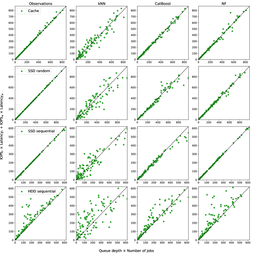
To verify the reliability of the models, we conducted an additional experiment. Relations between IOPS and latencies within the same data load are defined by Little’s law [18]:
| (18) |
where is the queue depth and is the number of jobs. For each data load in test samples, we calculated the right part of this equation and compared it with the left part estimated from the load parameters. The results are provided in Figure 8. The plots demonstrate that Little’s law is satisfied for the real observations in all data sets used in this study as well as for predictions of CatBoost and NF models. They learn the dependency in Equation 18 directly from the data. Table 10 provides Pearson’s correlation coefficients between the measurements in Figure 8. It shows that the coefficients for real observations, and predictions of CatBoost and NF models are similar, and support the reliability of the models. The kNN demonstrates larger differences from Little’s law than other models.
Figure 8 also shows that CatBoost and NF predictions for several data loads deviate significantly from the law. In such cases, the prediction errors are too large and we cannot trust them in decision-making. Therefore, Equation 18 can be used to verify the predictions of the models and to filter the predictions that are too bad.
| Sample | Observations | kNN | CatBoost | NF |
|---|---|---|---|---|
| Cache | 0.99 | 0.96 | 0.99 | 0.99 |
| SSD rand. | 0.99 | 0.92 | 0.97 | 0.99 |
| SSD seq. | 0.99 | 0.89 | 0.99 | 0.99 |
| HDD seq. | 0.91 | 0.72 | 0.92 | 0.89 |
Discussion

The results in the previous section show that generative models are suitable for performance modeling tasks. They are able to simulate the performance of a data storage system and its components for the given data load and configuration of the system. The models learn the conditional distribution of IOPS and latency, which can be used to predict their average values, as well as to estimate the variance of the predictions, confidence intervals, and other useful statistics.
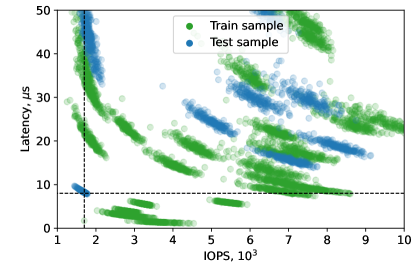
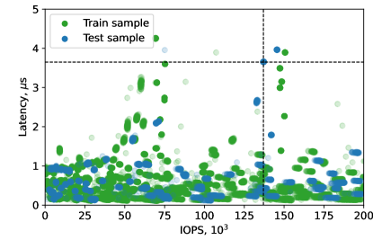
Samples with high error values tend to be near the boundary of the training data space, where the model operates in an extrapolation regime. An example of this behavior in the HDD predictions is presented in Figure 9, where one test data sample is indicated by the crosshairs (dashed lines), which is zoomed in in Figure 10. The predictions for this particular sample are also shown in this plot. This sample demonstrates what we call model conservatism, which is an instance of a model’s predictions being biased and shifted towards the training data in case the test data sample is the extrapolation regime. This figure represents the predictions being shifted toward the test samples, which shows that the model is consistent with the data on which it was trained.
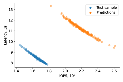
The same pattern of behavior is demonstrated in Figure 11. Here, the crosshairs are pointed on the test sample which is focused on in Figure 12 together with the predictions. It is observed that the predictions are located close to the test samples with the latter being in the extrapolation regime. This is another example of the model conservatism.
Conclusion
This work shows the results of the performance modeling of a data storage system using generative models. The outcomes help to conclude the following statements:
-
•
Generative models are reasonable alternatives to other methods for performance modeling studies. This approach is suitable for single devices and their combinations.
-
•
Both parametric and nonparametric models demonstrate similar prediction qualities for mean IOPS and latency values. But the parametric model estimates the standard deviations better.
-
•
The models can be used to predict the performance of a data storage system and its components for the given data load and configuration parameters.
-
•
The task has an unsupervised way for prediction reliability check based on Little’s law. The models we consider in this paper demonstrate this liability.
-
•
We provide real measurements of IOPS and latency for the cache, SSD, and HDD pools of a data storage system. This data set can be used in future works in the field of data-driven performance modeling and studies related to conditional generative models, uncertainty estimation, and model reliability.
Scripts of all our experiments in this work and all data sets are provided in the GitHub repository222https://github.com/HSE-LAMBDA/digital-twin.
Acknowledgments
The publication was supported by the grant for research centers in the field of AI provided by the Analytical Center for the Government of the Russian Federation (ACRF) in accordance with the agreement on the provision of subsidies (identifier of the agreement 000000D730321P5Q0002) and the agreement with HSE University No. 70-2021-00139.
The computation for this research was performed using the computational resources of HPC facilities at HSE University [26].
References
- [1] James Byron, Darrell D.. Long and Ethan L. Miller “Using Simulation to Design Scalable and Cost-Efficient Archival Storage Systems” In 2018 IEEE 26th International Symposium on Modeling, Analysis, and Simulation of Computer and Telecommunication Systems (MASCOTS), 2018 IEEE DOI: 10.1109/mascots.2018.00011
- [2] Yang Li, Li Guo and Yike Guo “An Efficient and Performance-Aware Big Data Storage System” In Communications in Computer and Information Science Springer International Publishing, 2013, pp. 102–116 DOI: 10.1007/978-3-319-04519-1˙7
- [3] H. Huang, Shan Li, Alex Szalay and Andreas Terzis “Performance Modeling and Analysis of Flash-Based Storage Devices” In 2011 IEEE 27th Symposium on Mass Storage Systems and Technologies (MSST), 2011, pp. 1–11 DOI: 10.1109/MSST.2011.5937213
- [4] Shan Li and H. Huang “Black-Box Performance Modeling for Solid-State Drives” In 2010 IEEE International Symposium on Modeling, Analysis and Simulation of Computer and Telecommunication Systems Miami Beach, FL, USA: IEEE, 2010, pp. 391–393 DOI: 10.1109/MASCOTS.2010.48
- [5] Joonsung Kim, Kanghyun Choi, Wonsik Lee and Jangwoo Kim “Performance Modeling and Practical Use Cases for Black-Box SSDs” In ACM Transactions on Storage 17.2, 2021, pp. 14:1–14:38 DOI: 10.1145/3440022
- [6] Mojtaba Tarihi et al. “Quick Generation of SSD Performance Models Using Machine Learning” In IEEE Transactions on Emerging Topics in Computing 10.4, 2022, pp. 1821–1836 DOI: 10.1109/TETC.2021.3116197
- [7] Zhimin Zeng, Xinyu Chen, Laurence T. Yang and Jinhua Cui “IMRSim: A Disk Simulator for Interlaced Magnetic Recording Technology” arXiv, 2022 DOI: 10.48550/arXiv.2206.14368
- [8] Myoungsoo Jung et al. “SimpleSSD: Modeling Solid State Drives for Holistic System Simulation” In IEEE Computer Architecture Letters 17.1, 2018, pp. 37–41 DOI: 10.1109/LCA.2017.2750658
- [9] Donghyun Gouk et al. “Amber*: Enabling precise full-system simulation with detailed modeling of all ssd resources” In 2018 51st Annual IEEE/ACM International Symposium on Microarchitecture (MICRO), 2018, pp. 469–481 IEEE
- [10] Youngjae Kim, Brendan Tauras, Aayush Gupta and Bhuvan Urgaonkar “FlashSim: A Simulator for NAND Flash-Based Solid-State Drives” In 2009 First International Conference on Advances in System Simulation, 2009, pp. 125–131 DOI: 10.1109/SIMUL.2009.17
- [11] Eric M Jayson, James M Murphy, Paul W Smith and Frank E Talke “Shock and head slap simulations of operational and nonoperational hard disk drives” In IEEE transactions on magnetics 38.5 IEEE, 2002, pp. 2150–2152
- [12] Yongkun Li, Patrick PC Lee and John CS Lui “Stochastic modeling of large-scale solid-state storage systems: Analysis, design tradeoffs and optimization” In Proceedings of the ACM SIGMETRICS/international conference on Measurement and modeling of computer systems, 2013, pp. 179–190
- [13] Jangryul Kim and Soonhoi Ha “Fast Performance Estimation and Design Space Exploration of SSD Using AI Techniques” In Embedded Computer Systems: Architectures, Modeling, and Simulation, Lecture Notes in Computer Science Cham: Springer International Publishing, 2020, pp. 1–17 DOI: 10.1007/978-3-030-60939-9˙1
- [14] Yoonsuk Kang et al. “A Framework for Estimating Execution Times of IO Traces on SSDs” In Proceedings of the 2017 ACM on Conference on Information and Knowledge Management Singapore Singapore: ACM, 2017, pp. 2123–2126 DOI: 10.1145/3132847.3133115
- [15] “Perf: Linux profiling with performance counters” Accessed: 2022-01-12, https://perf.wiki.kernel.org/index.php/Main_Page
- [16] Il’ya Meerovich Sobol’ “On the distribution of points in a cube and the approximate evaluation of integrals” In Zhurnal Vychislitel’noi Matematiki i Matematicheskoi Fiziki 7.4 Russian Academy of Sciences, Branch of Mathematical Sciences, 1967, pp. 784–802
- [17] Anna Veronika Dorogush, Vasily Ershov and Andrey Gulin “CatBoost: gradient boosting with categorical features support” arXiv, 2018 DOI: 10.48550/ARXIV.1810.11363
- [18] John D.. Little “A Proof for the Queuing Formula: L= W” In Operations Research 9.3 INFORMS, 1961, pp. 383–387 URL: http://www.jstor.org/stable/167570
- [19] Gene H. Golub and Charles F. Van Loan “Matrix Computations (3rd Ed.)” USA: Johns Hopkins University Press, 1996
- [20] George Papamakarios et al. “Normalizing Flows for Probabilistic Modeling and Inference” In Journal of Machine Learning Research 22.57, 2021, pp. 1–64 URL: http://jmlr.org/papers/v22/19-1028.html
- [21] Laurent Dinh, Jascha Sohl-Dickstein and Samy Bengio “Density estimation using Real NVP” arXiv, 2016 DOI: 10.48550/ARXIV.1605.08803
- [22] D.C Dowson and B.V Landau “The Fréchet distance between multivariate normal distributions” In Journal of Multivariate Analysis 12.3, 1982, pp. 450–455 DOI: https://doi.org/10.1016/0047-259X(82)90077-X
- [23] Martin Heusel et al. “GANs Trained by a Two Time-Scale Update Rule Converge to a Local Nash Equilibrium” In Proceedings of the 31st International Conference on Neural Information Processing Systems, NIPS’17 Long Beach, California, USA: Curran Associates Inc., 2017, pp. 6629–6640
- [24] Arthur Gretton et al. “A Kernel Two-Sample Test” In Journal of Machine Learning Research 13.25, 2012, pp. 723–773 URL: http://jmlr.org/papers/v13/gretton12a.html
- [25] F. Pedregosa et al. “Scikit-learn: Machine Learning in Python” In Journal of Machine Learning Research 12, 2011, pp. 2825–2830
- [26] P.. Kostenetskiy, R.. Chulkevich and V.. Kozyrev “HPC Resources of the Higher School of Economics” In Journal of Physics: Conference Series 1740.1 IOP Publishing, 2021, pp. 012050 DOI: 10.1088/1742-6596/1740/1/012050
Abdalaziz R. Al-Maeeni is a Ph.D. student and a Junior Research Fellow at the Faculty of Computer Science, HSE University, Russia. His main research interests are interpretable generative models and inverse design. Contact him at al-maeeni@hse.ru.
Aziz Temirkhanov is a Master’s student at the Faculty of Computer Science, HSE University, Russia. His main research interests are generative models and its application in natural science.
Artem Ryzhikov is a Ph.D. student and a Junior Research Fellow at the Faculty of Computer Science, HSE University, Russia. His research interests are in the area of machine learning and its application to High-Energy Physics with a focus on Deep Learning and Bayesian methods.
Mikhail Hushchyn is a Senior Research Fellow at the Faculty of Computer Science, HSE University, Russia. His main research interests include the application of machine learning and artificial intelligence methods in the natural sciences and industry. He is the corresponding author. Contact him at mhushchyn@hse.ru.