Empirical Bayes via ERM and Rademacher complexities: the Poisson model

Abstract

We consider the problem of empirical Bayes estimation for (multivariate) Poisson means. Existing solutions that have been shown theoretically optimal for minimizing the regret (excess risk over the Bayesian oracle that knows the prior) have several shortcomings. For example, the classical Robbins estimator does not retain the monotonicity property of the Bayes estimator and performs poorly under moderate sample size. Estimators based on the minimum distance and non-parametric maximum likelihood (NPMLE) methods correct these issues, but are computationally expensive with complexity growing exponentially with dimension. Extending the approach of [BZ22], in this work we construct monotone estimators based on empirical risk minimization (ERM) that retain similar theoretical guarantees and can be computed much more efficiently. Adapting the idea of offset Rademacher complexity [LRS15] to the non-standard loss and function class in empirical Bayes, we show that the shape-constrained ERM estimator attains the minimax regret within constant factors in one dimension and within logarithmic factors in multiple dimensions.

1 Introduction

At the heart of modern large-scale inference [Efr12], empirical Bayes is a classical topic and powerful formalism in statistics and machine learning. Consider the Poisson model in one dimension as a concrete example. In a Bayesian setting, the latent parameter $\theta$ is drawn from a prior $\pi$ and the observation $X$ is then sampled from $\mathrm{Poi}(\theta)$, the Poisson distribution with mean $\theta$. In other words, $X$ is distributed according to the following Poisson mixture $p_{\pi}$ with mixing distribution $\pi$:

$$p_{\pi}(x)=\int{e^{-\theta}{\theta^{x}\over x!}}d\pi(\theta),\quad x\in\mathbb{Z}_{+}.$$ (1)

The Bayes estimator for $\theta$ that minimizes the squared error is the posterior mean, which can be expressed in terms of the mixture density as follows:

$$f^{*}(x)=(x+1){p_{\pi}(x+1)\over p_{\pi}(x)}$$ (2)

In the empirical Bayes setting, the prior $\pi$ is unknown but we have access to a training sample $X_{1},\dots,X_{n}$ drawn independently from the mixture $p_{\pi}$. The goal is to learn a data-driven rule that produces vanishing excess risk over the Bayes risk, known as the regret

$$\mathsf{Regret}_{\pi}(f)\triangleq\mathbb{E}\left[(\widehat{f}(X)-\theta)^{2}\right]-\mathbb{E}\left[(f^{*}(X)-\theta)^{2}\right].$$ (3)

The problem of interest in this context is thus:

Can we construct computationally efficient and practically sound estimators of $f^{*}$ with optimal regret over a class of priors?

Preliminary analyses of the Poisson empirical Bayes problem go back to [Rob51, Rob56], who proposed the following rule as an empirical approximation of (2):

$$\widehat{f}_{\mathsf{Rob}}(X)\triangleq\widehat{f}_{\mathsf{Rob}}(X;X_{1},\dots,X_{n})=(X+1){N_{n}(X+1)\over N_{n}(X)+1}$$ (4)

where $N_{n}(x)=\sum_{i=1}^{n}{\mathbf{1}_{\left\{{X_{i}=x}\right\}}}$ is the empirical count for each $x\in\mathbb{Z}_{+}$ in the training sample. Such an approach is termed “$f$-modeling” that focuses on approximating the mixture density [Efr14]. Recent theoretical developments [BGR13, PW20] have established that the Robbins method achieves the optimal rate of regret when $\pi$ has either bounded support or subexponential tails. On the other hand, in practice, it is well-recognized that the Robbins estimator suffers from multiple shortcomings such as numerical instability (cf. e.g. [Mar68, Section 1], [ML18, Section 1.9], [EH21, Section 6.1]) and lack of regularity properties, including, notably, the desired monotonicity property of the Bayes rule $f^{*}$ (see [HS83]).

In another approach to the empirical Bayes problem, known as “$g$-modeling” [Efr14], one tries to mimic the structure of the Bayes estimator by substituting the prior in the posterior mean with a suitable estimator. It has recently been shown that optimal regret can be attained by $g$-modeling estimators based on the minimum distance methodology that first finds the best approximation $p_{\widehat{\pi}}$ to the empirical distribution of the training data under suitable distances then applies the Bayes rule with the learned prior $\widehat{\pi}$. A prominent example is the nonparametric maximum likelihood estimator (NPMLE)

$$\widehat{\pi}_{\sf NPMLE}=\mathop{\rm argmax}_{Q}\prod_{i=1}^{n}p_{Q}(X_{i})$$ (5)

which minimizes the Kullback-Leibler divergence. Thanks to their Bayesian form, these estimators inherit the desired regularity of Bayes estimator (such as monotonicity) and lead to more stable, accurate, and interpretable estimates in practice. Recently, [JPW22] has shown that a suite of minimum-distance estimators, including the NPMLE, attain the optimal regret similar to the Robbins estimator for both bounded or subexponential priors. In addition, when $\pi$ has heavier (polynomial) tails, the NPMLE achieves the corresponding optimal regret while Robbins estimator provably fails [SW22]. However, the downside of $g$-modeling is its much higher computational cost. For example, (5) entails solving an infinite-dimensional convex optimization. Although in one dimension faster algorithms akin to Frank-Wolfe have been proposed [Lin83, JPW22], for multiple dimensions existing solvers essentially all boil down to maximizing the weights over a discretized domain [KM14] which clearly does not scale with the dimension.

1.1 Empirical Bayes via Empirical Risk Minimization

In this paper we propose a new approach for Poisson empirical Bayes by incorporating a framework based on empirical risk minimization (ERM) and the needed technology from learning theory, notably, the offset Rademacher complexity, refined via localization, to establish the optimality of the achieved regret. In contrast to $f$-modeling and $g$-modelling that aim at approximating the mixture density and the prior respectively, the main idea is to directly approximate the Bayes rule by solving a suitable ERM subject to certain structural constraints satisfied by the Bayesian oracle. We note that a similar technique has been applied earlier in [BZ22] to the Gaussian model; however, the theoretical guarantees therein are highly suboptimal.

The benefits of the ERM-based methodology are manifold:

1. Unlike the Robbins method, the constrained ERM produces an estimator that enjoys the same regularity as that of the Bayes rule, at a small permillage of the computational cost of $g$-modeling methods such as the NPMLE and other minimum-distance estimators.

2. The ERM-based estimator is scalable to high dimensions and runs in time that is polynomial in both $n$ and the dimension $d$. In contrast, all existing algorithms for NPMLE are essentially grid-based and scales poorly with the dimension as $n^{\Theta(d)}$.

3. The ERM approach invites powerful tools from empirical processes theory (such as Rademacher complexity and variants) to bear on its regret.

4. The flexibility of the ERM framework allows one to easily incorporate extra constraints or replace the function class by more powerful ones (such as neural nets) in order to tackle more challenging empirical Bayes problems in high dimensions for which there is no feasible proposal so far.

To summarize, the ERM can be seen as an alternative solution to the empirical Bayes problem, that excels over the Robbins method in terms of retaining the regularity properties of the Bayes estimator, and is computationally much efficient than the other existing non-parametric alternatives. We will also show that theoretically it achieves the optimal regret for certain light-tailed classes of priors. Whether these guarantees carry over to the heavy-tailed classes of prior, where the Robbins method is known to be suboptimal and NPMLE is known to be optimal [SW22], is beyond the scope of the current paper.

Next we describe the construction of the ERM-based empirical Bayes estimator in details. To derive the objective function for the ERM, note that using $f^{*}(X)=\mathbb{E}\left[\theta|X\right]$, we have

$$f^{*}=\mathop{\rm argmin}_{f}\mathbb{E}[(f(X)-\theta)^{2}] =\mathop{\rm argmin}_{f}\mathbb{E}[(f(X))^{2}-2\theta f(X)]$$

$$=\mathop{\rm argmin}_{f}\mathbb{E}\left[f(X)^{2}-2Xf(X-1)\right],$$

where we get the last step applying the identity $\mathbb{E}\left[\theta f(X)\right]=\mathbb{E}\left[Xf(X-1)\right]$ for $X\sim\mathrm{Poi}(\theta)$. Since $f^{*}$ is monotone, this naturally leads to the ERM-based estimator

$$\widehat{f}_{\mathsf{erm}}\in\mathop{\rm argmin}_{f\in{\mathcal{F}}}\widehat{\mathbb{E}}[f(X)^{2}-2Xf(X-1)],$$ (6)

where $\widehat{\mathbb{E}}[h(X)]\triangleq\frac{1}{n}\sum_{i=1}^{n}h(X_{i})$ denotes the empirical expectation of a function $h$ based on the sample $X_{1},\dots,X_{n}$, and the minimization (6) is over the class of monotone functions ${\mathcal{F}}=\{f:f(x)\leq f(x+1),\forall x\geq 0\}$. We also note that the solution (6) is only uniquely specified on the set $S\triangleq\{X_{1},\ldots,X_{n}\}\cup\{X_{1}-1,\ldots,X_{n}-1\}$, which can be easily computed by an algorithm akin to isotonic regression (see Lemma 1). We then extend this solution to the whole $\mathbb{Z}_{+}$ in a piecewise constant manner: for those $x<\min S$, set $\widehat{f}_{\mathsf{erm}}(x)=0$; for those $x>\max S=X_{\max}\triangleq\max\{X_{1},\ldots,X_{n}\}$, set $f(x)=f(X_{\max})$; for the remaining $x\not\in S$, set $\widehat{f}_{\mathsf{erm}}(x)=\widehat{f}_{\mathsf{erm}}(\max\{y\in S:y\leq x\})$. This natural piecewise constant extension clearly retains monotonicity.

We note that the above construction of the ERM-based empirical Bayes estimator can be done in a principled way for other mixture models than Poisson (see Table 1). Indeed, [BZ22] was the first to apply this approach to the Gaussian mixture model. However, only the slow rate of $\frac{\mathsf{polylog}(n)}{\sqrt{n}}$ is obtained for the regret by applying standard empirical process theory. In addition, they use extra constraints, such as the ones based on bounded derivatives, bounds on the parameter space, etc. These constraints can be used to further improve upon the practical performances of the ERM estimator we use for the Poisson model; however the corresponding analysis is beyond the scope of the current paper. One of the major technical contributions of the present paper is to introduce a suitable version of the offset Rademacher complexity [LRS15] that leads to the fast rate of $\frac{\mathsf{polylog}(n)}{n}$ (even with the optimal logarithmic factors!)

Mixture	$p(X|\theta)$	Bayes estimator	ERM Objective
Geo$(\theta)$	$\theta^{X}(1-\theta)$	$1-\frac{p_{\pi}(X+1)}{p_{\pi}(X)}$	$\widehat{\mathbb{E}}[f(X)^{2}-2f(X)+2f(X-1){\mathbf{1}_{\left\{{X>0}\right\}}}]$
NB$(r,\theta)$	$\binom{k+r-1}{k}(1-\theta)^{r}\theta^{k}$	$\frac{X+1}{X+r}\frac{p_{\pi}(X+1)}{p_{\pi}(X)}$	$\widehat{\mathbb{E}}[f(X)^{2}-2\frac{X+1}{X+r}f(X-1){\mathbf{1}_{\left\{{X>0}\right\}}}]$
$\mathcal{N}(\theta,1)$	$\frac{1}{\sqrt{2\pi}}\mathop{\rm exp}\left(-\frac{(X-\theta)^{2}}{2}\right)$	$X+\frac{p^{\prime}_{\pi}(X)}{p_{\pi}(X)}$	$\widehat{\mathbb{E}}[f(X)^{2}-2Xf(X)+2f^{\prime}(X)]$
$\text{Exp}(\theta)$	$\theta\mathop{\rm exp}(-\theta X)$	$-\frac{p^{\prime}_{\pi}(X)}{p_{\pi}(X)}$	$\widehat{\mathbb{E}}[f(X)^{2}-2f^{\prime}(X)]$

Table 1: ERM objectives for other mixture models: geometric, negative binomial, normal location, and exponential distributions.

1.2 Regret optimality

In addition to its conceptual simplicity and computational advantage, the ERM-based estimator comes with strong statistical guarantees which we now describe. Let ${\mathcal{P}}[0,h]$ denote the class of all priors supported on the interval $[0,h]$ and $\mathsf{SubE}(s)$ the set of all $s$-subexponential distributions on $\mathbb{R}_{+}$, namely $\mathsf{SubE}(s)=\left\{G:G([t,\infty)])\leq 2e^{-t/s},\forall t>0\right\}$. Our main result is as follows:

Theorem 1 (Regret optimality of ERM-based estimators).

Let $\widehat{f}_{\mathsf{erm}}$ be defined in (6), with ${\mathcal{F}}$ the class of all monotone functions on $\mathbb{Z}_{+}$. Then there exist s a constant $C>0$ such that for any $h,s>0$,

$$\sup_{\pi\in{\mathcal{P}}([0,h])}\mathsf{Regret}_{\pi}(\widehat{f}_{\mathsf{erm}})\leq\frac{C\max\{1,h\}^{3}}{n}\left(\log n\over\log\log n\right)^{2},\quad\sup_{\pi\in{\mathsf{SubE}(s)}}\mathsf{Regret}_{\pi}(\widehat{f}_{\mathsf{erm}})\leq\frac{C\max\{1,s\}^{3}}{n}(\log n)^{3}.$$

The regret bounds in Theorem 1 match the minimax lower bounds in [PW21, Theorem 2] up to constant factors, thereby establish the strong optimality of the ERM-based empirical Bayes estimators. Finally, as a side remark, we mention that, one can show that a monotone projection of the Robbins estimator, given by $\widehat{f}_{\text{\sf mono-Rob}}=\mathop{\rm argmin}_{f\in{\mathcal{F}}}\widehat{\mathbb{E}}[(f(X)-\widehat{f}_{\mathsf{Rob}}(X))^{2}]$, also attains similar regret guarantees as in Theorem 1. This is outside the scope of the current paper.

1.3 Multiple dimensions

The ERM-based estimator (6) can be easily extended to the $d$-dimension Poisson model. For clarity, we use the bold fonts to denote a vector, e.g., $\bm{\theta}=\left(\theta_{1},\dots,\theta_{d}\right),\bm{\theta}_{i}=(\theta_{i1},\dots,\theta_{id}),\bm{X}=(X_{1},\dots,X_{d}),\bm{X}_{i}=(X_{i1},\dots,X_{id}),\bm{x}=(x_{1},\dots,x_{d})$, etc. Let $\pi$ be a prior distribution on $\mathbb{R}_{+}^{d}$. Consider the following data-generating process

$$\bm{\theta}_{i}{\stackrel{{\scriptstyle\text{iid}}}{{\sim}}}\pi\qquad X_{ij}{\stackrel{{\scriptstyle\text{ind.}}}{{\sim}}}\mathrm{Poi}(\theta_{ij}).$$ (7)

Note that the marginal distribution of the multidimensional Poisson mixture is given by

$$p_{\pi}(\bm{x})=\int_{\bm{\theta}}\prod_{i=1}^{d}e^{-\theta_{i}}{\theta_{i}^{x_{i}}\over x_{i}!}d\pi(\bm{\theta}),\quad\bm{x}\in\mathbb{Z}_{+}^{d}.$$

Similar to (3), let us define the regret of a given estimator $\bm{f}:\mathbb{Z}_{+}^{d}\to\mathbb{R}_{+}^{d}$ as

$$\mathsf{Regret}_{\pi}(\bm{f})=\mathbb{E}\left[\|\bm{f}(\bm{X})-\bm{\theta}\|^{2}\right]-\mathbb{E}\left[\|\bm{f}^{*}(\bm{X})-\bm{\theta}\|^{2}\right],$$ (8)

where $\bm{X}\sim p_{\pi}$ is a test point independent from the training sample $\bm{X}_{1},\ldots,\bm{X}_{n}{\stackrel{{\scriptstyle\text{iid}}}{{\sim}}}p_{\pi}$. For each $\bm{f}$, let $\bm{f}=(f_{1},\cdots,f_{d})$ where $f_{i}:\mathbb{Z}_{+}^{d}\to\mathbb{R}_{+}$. Denote by $\bm{f}^{*}$ the Bayes estimator, whose $i$-th coordinate $f_{i}^{*}$ is given by

$$f^{*}_{i}(\bm{x})=\mathbb{E}[\theta_{i}|\bm{x}]={\int_{\bm{\theta}}\theta_{i}\prod_{j=1}^{d}e^{-\theta_{i}}{\theta_{i}^{x_{i}}\over x_{i}!}d\pi(\bm{\theta})\over p_{\pi}(\bm{x})}=(x_{i}+1)\frac{p_{\pi}(\bm{x}+\bm{e}_{i})}{p_{\pi}(\bm{x})},\quad i=1,\dots,d,$$

where $\bm{e}_{i}$ denote the $i$-th coordinate vector. Using Cauchy-Schwarz, one can show that the Bayes estimator for the $i$-th coordinate is increasing in the $i$-th coordinate of the input if all other coordinates are fixed, i.e.,

$$f^{*}_{i}(\bm{x})\leq f^{*}_{i}(\bm{x}+\bm{e}_{i}),\quad\forall i=1,\dots,d,\quad\forall\bm{x}\in\mathbb{Z}_{+}^{d}$$ (9)

This leads to the following ERM procedure.

$$\widehat{\bm{f}}_{\mathsf{erm}} =\mathop{\rm argmin}_{\bm{f}\in\bm{\mathcal{F}}}\quad\widehat{\mathbb{E}}\left[{\left\|\bm{f}(\bm{X})\right\|}^{2}-2\sum_{j=1}^{d}X_{j}f_{j}(\bm{X}-\bm{e}_{i})\right],$$

$$\bm{\mathcal{F}}= \{\bm{f}:\mathbb{Z}_{+}^{d}\to\mathbb{R}_{+}^{d}:f_{i}(\bm{x})\leq f_{i}(\bm{x}+\bm{e}_{i}),\forall i=1,\cdots,d,\forall\bm{x}\in\mathbb{Z}_{+}^{d}\}.$$ (10)

We again note that $\widehat{\bm{f}}_{\mathsf{erm}}$ is not uniquely defined for all $\bm{x}\in\mathbb{Z}_{+}^{d}$. To specify a minimizer, note that $(\widehat{f}_{\mathsf{erm}})_{j}$, the $j$-th coordinate of $\widehat{\bm{f}}_{\mathsf{erm}}$, is uniquely defined on $S\triangleq\{\bm{X}_{i}\}\cup\{\bm{X}_{i}-\bm{e}_{j}\}$. We may extend it to $\mathbb{Z}_{+}^{d}$ in the same manner as the one-dimensional case of (6) in a piecewise constant manner. That is, for each $\bm{x}\not\in S$, if there exists $y\geq 0$ such that $\bm{x}-y\bm{e}_{j}\in S$, we set $(\widehat{f}_{\mathsf{erm}})_{j}(\bm{x})=(\widehat{f}_{\mathsf{erm}})_{j}(\min_{y\geq 0\atop\bm{x}-y\bm{e}_{j}\in S}\bm{x}-y\bm{e}_{j})$. Otherwise, set $(\widehat{f}_{\mathsf{erm}})_{j}(\bm{x})=0$. By convention, we also define $(\widehat{f}_{\mathsf{erm}})_{j}(-\bm{e}_{j})=0$.

Theorem 2.

The ERM estimator (1.3) satisfies the following regret bounds whenever $n\geq d$:

1. If $\pi$ is supported on $[0,h]^{d}$, then $\mathsf{Regret}_{\pi}(\widehat{\bm{f}}_{\mathsf{erm}})\leq O(\frac{d}{n}\max\{c_{1},c_{2}h\}^{d+2}(\frac{\log(n)}{\log\log(n)})^{d+1})$ ;

2. If all marginals of $\pi$ are $s$-subexponential for some $s>0$, then
   $\mathsf{Regret}_{\pi}(\widehat{\bm{f}}_{\mathsf{erm}})\leq O(\frac{d}{n}{(\max\{c_{3},c_{4}s\}\log(n))^{d+2}})$,

where $c_{1},c_{2},c_{3},c_{4}>0$ are absolute constants.

We conjecture these regret bounds in Theorem 2 are nearly optimal and factors like $(\log n)^{d}$ are necessary. Indeed, for the Gaussian model in $d$ dimensions, the minimax squared Hellinger risk for density estimation is shown to be at least $O((\log n)^{d}/n)$ for subgaussian mixing distributions and the minimax regret is typically even larger. A rigorous proof of matching lower bound for Theorem 2 will likely involve extending the regret lower bound based on Bessel kernels in [PW21] to multiple dimensions; this is left for future work.

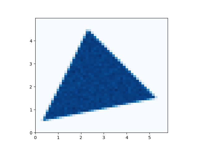
(a) Latent $\bm{\theta}_{i}$’s.

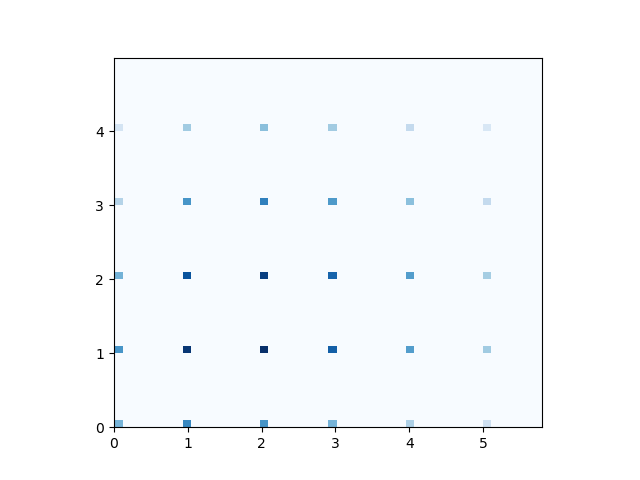
(b) Observations $\bm{X}_{i}$’s.

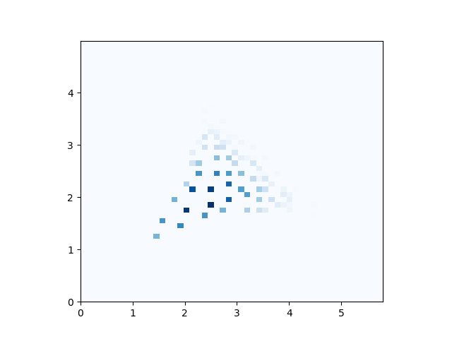
(c) Denoised $\widehat{\bm{f}}_{\mathsf{erm}}$.

Figure 1: A two-dimensional experiment with $n=10^{6}$: Left: $\bm{\theta}_{i}$’s are sampled uniformly from a triangle. Middle: the observations $\bm{X}_{i}$’s are drawn independently from $\mathrm{Poi}(\bm{\theta}_{i})$, with their empirical distribution shown on the grid $\mathbb{Z}_{+}^{2}$ (notice that this is also the MLE estimator for $\bm{\theta}$, hence very different from the empirical Bayes solution). Right: the empirical Bayes denoised version obtained by applying $\widehat{f}_{\mathsf{erm}}$ in (1.3) to $\bm{X}_{i}$’s.

Remark 1 (Time complexity).

For the statistical rate of ERM in multiple dimensions to be meaningful, we require $d$ to be significantly smaller than $n$. Nonetheless, even in the dimensions where the regret in Theorem 2 is vanishing, the ERM method is computationally much more scalable, compared with the conventional approach based on NPMLE or other minimum-distance estimators.

To elaborate on this, ERM is a linear program and has a dedicated solver due to its special form. NPMLE is an infinite-dimensional convex optimization, and the prevailing solver either discretizes the domain (at least $\sqrt{n}$ level in order to be statistically relevant, thus requires a grid of size $n^{\Theta(d)}$) or runs Frank-Wolfe style iteration, which is only known to converge slowly at $\frac{1}{t}$ rate [Lin83] and requires mode finding that is expensive in multiple dimensions. In contrast, the ERM approach scales much better with the dimension. To evaluate the $d$-dimensional ERM (1.3), as we will demonstrate in Remark 4, if $\ell$ is the number of distinct vector-valued observations $\bm{X}_{1},\ldots,\bm{X}_{n}$, our algorithm runs in $O(d\ell^{2})\leq O(dn^{2})$ time (apart from reading the sample of size $n$). An almost linear time $O(d\ell\log\ell)$ algorithm (which is how we implemented in the simulations), exists but is beyond the scope of this paper. (We will describe the basic idea in Appendix B.)

On the empirical side, we demonstrate the multidimensional feasibility of ERM by running a simulation with $\bm{\theta}_{1},\ldots,\bm{\theta}_{n}$ sampled uniformly from a triangle with $n=10^{6}$ and compute the empirical Bayes denoiser $\widehat{\bm{f}}_{\mathsf{erm}}$ in (1.3) to $\bm{X}_{i}{\stackrel{{\scriptstyle\text{ind.}}}{{\sim}}}\mathrm{Poi}(\bm{\theta}_{i})$. Here, we see that $\widehat{\bm{f}}_{\mathsf{erm}}$ can recover the triangular structure of the prior, as in Fig. 1. To further compare the computational costs of ERM and minimum distance methods, we did a comparison in the statistical software $R$ with the popular package “REBayes” [KG17] and the results are as follows. With the prior $\mathsf{Unif}(4,30)$ and sample sizes $n=50,500,5000,50000$, we ran both REBayes and ERM 100 times and found that on average the ERM is respectively $21,50,212,588$ times faster. This improvement is even more pronounced ($25,58,227.5,2160$ times) if we supply the empirical distribution to the ERM instead of the full sample.

Remark 2 (Comparison with $f$-modelling).

While both $f$-modelling (i.e. the Robbins estimator) and the ERM estimator $\widehat{f}_{\mathsf{erm}}$ are asymptotically optimal, we demonstrate more concretely the advantage of $\widehat{f}_{\mathsf{erm}}$ over Robbins. The shortcomings of the Robbins method have been widely observed in practice and discussed in the existing literature. Most recently, it has been demonstrated in [JPW22] extensively through both simulated and real data experiment. Expanding on Fig. 1(a), which compares the performance of the multidimensional Robbins method and $\widehat{f}_{\mathsf{erm}}$ under a uniform prior on the 2d triangle, for $n=10^{k},k=4,5,6,7$, we found that the Robbins method achieved a regret of $0.356,0.0575,0.00771,0.00116$ and $\widehat{f}_{\mathsf{erm}}$ achieved a regret of $0.0748,0.0161,0.00276,0.000463$, suggesting a much better performance. On another experiment, we also compared the methods in dimensions $1,2,3,4$ using a product of $\text{Exp}(2)$ distributions as prior, fixing $n=10000$. The Robbins method achieved regrets $0.0125,0.0607,0.185,0.427$; $\widehat{f}_{\mathsf{erm}}$ achieved regrets $0.00422,0.0208,0.0660,0.161$.

1.4 Related work

Empirical Bayes estimation for the Poisson means incorporating shape constraint has a long research thread. However, the majority of the work relies on approximating the Robbins estimator using monotone functions. For example, [Mar66] used linear approximation to the Robbins estimator and [Mar69] represented the marginal distribution $p_{\pi}$ based on a monotone ordinate fit to the Robbins and then used it to compute a maximum likelihood estimation of the ordinates. Both of these papers focus on numerical comparison of the corresponding error guarantees; see [ML18, Section 3.4.5] for a concise exposition. In recent work, [BGR13] discussed the numerical benefits of first performing a Rao-Blackwellization on the Robbins estimator and then using an isotonic regression to impose the monotonicity of the final estimator. An important theoretical contribution to the monotone smoothing of any given empirical Bayes estimator has been proposed in [VH77]. Using the monotone likelihood ratio property of the Poisson distribution, it is shown that any estimator (e.g., the Robbins estimator) can be made monotone without increasing the regret. In contrast, our main estimator is computed directly via minimizing an empirical version of the regret. It might be possible to use the monotone smoothing of [VH77] to further improve the ERM-estimator which is not pursued in this work.

As mentioned in Section 1.1, the application of empirical risk minimization in empirical Bayes has been introduced in the one-dimensional normal mean model by [BZ22]. Using the monotonicity of the posterior mean, they construct an empirical Bayes estimator by solving the ERM under monotonicity constraint (see Table 1). However, the regret bound they establish is of the slow rate $\mathsf{polylog}(n)\over\sqrt{n}$ which is highly suboptimal, compared with the nearly optimal rate of $O(\frac{(\log n)^{5}}{n})$ by [JZ09] (based on the $g$-modeling approach via NPMLE) and $O(\frac{(\log n)^{8}}{n})$ by [LGL05] (based on the $f$-modeling approach of polynomial kernel density estimates). As mentioned earlier, the NPMLE is computationally expensive, especially in multiple dimensions due to the reliance on grid-based approximation [KM14, SGS21]. In contrast, as mentioned before, ERM-based estimators algorithm can be easily constructed for multiple or high dimensions.

The rest of the paper is organized as follows. Section 2 provides a regret upper bound on the ERM-based estimator in one dimension in terms of the offset Rademacher complexities, and a proof sketch for Theorem 1. Section 3 contains the analysis for the multidimensional ERM-estimator and a proof sketch of Theorem 2. Omitted proofs are provided in the appendices.

2 Regret guarantees for the ERM estimator via Offset Rademacher complexity

2.1 The ERM algorithm

As mentioned in the last section, our proposed estimator is based on ERM framework. In many statistical problems, the statistician intends to find a function $f$ that approximates a target statistic $s(X)$ in order to minimize the error $\mathbb{E}\left[\ell\left(s(X),f(X)\right)\right]$ for some suitable loss function $\ell$. In the ERM framework, the population average is replaced by the empirical average $\widehat{\mathbb{E}}\left[\ell\left(s(X);f(X)\right)\right]$ over the training sample. There is a rich literature on using such methods to approximate nonparametric target functions. See, for example, [Nem85, VdG90] for regression problems, [Bar91, BC91, Bar94] for penalized empirical risk minimization, [BM93, LZ95] for consistency results of general nonparametric ERM-estimators, etc. In this paper, we aim to approximate the nonparametric target function $f^{*}$ (the Bayes rule) by minimizing $\mathbb{E}\left[(f^{*}(X)-f(X))^{2}\right]$. As shown in Section 1.1, in the Poisson mixture model, this can be equivalently expressed as minimizing $\mathbb{E}\left[f(X)^{2}-2Xf(X-1)\right]$ and we minimize the corresponding empirical loss over the class of all monotone functions. Isotonic minimization of such quadratic loss is easy to compute; [BC90] showed that monotone projection can be done in linear time. In the following lemma we present one such minimization algorithm that we use in numerical analyses. The proof is deferred to Appendix B.

Lemma 1.

Let $a_{1}<\cdots<a_{n}$ be a sequence of non-negative integers and $\{v_{i}\}_{i=1}^{n},\{w_{i}\}_{i=1}^{n}$ be two non-negative sequences with $v_{n}>0$ and $\max\{v_{i},w_{i}\}>0$ for all $i$. Consider the iterative $b_{i}$

$$b_{i}=\begin{cases}1&i=0\\ 1+\mathop{\rm argmin}_{b_{i-1}\leq i^{*}\leq n}\frac{\sum_{i=b_{i-1}}^{i^{*}}w_{i}}{\sum_{i=b_{i-1}}^{i^{*}}v_{i}}&i\geq 1\\ \end{cases}$$

where the fraction is $+\infty$ whenever the denominator is 0, and where tie exists at $\mathop{\rm argmin}$, choose biggest such $i^{*}$. We stop at $b_{m}=n+1$. Then the solution to

$$\widehat{f}_{\mathsf{erm}}=\mathop{\rm argmin}_{f\in{\mathcal{F}}}\sum_{i=1}^{n}v_{i}f(a_{i})^{2}-2w_{i}f(a_{i})$$

is given as

$$\forall i=1,\cdots,m,\forall x:b_{m}\leq x<b_{m+1}:\widehat{f}_{\mathsf{erm}}(a_{x})=\frac{\sum_{i=b_{m}}^{b_{m+1}-1}w_{i}}{\sum_{i=b_{m}}^{b_{m+1}-1}v_{i}}.$$

Remark 3.

Making the restriction $v_{i}\geq 0$ and $v_{n}>0$ ensures that our solution will be well-formed. To apply this algorithm to estimate $\widehat{f}_{\mathsf{erm}}$, let $\{a_{1},\cdots,a_{k}\}\subseteq\{1,\cdots,X_{\max}\}$ be such that either $N(a_{i})>0$ or $N(a_{i}+1)>0$. Here, $v_{i}=N(a_{i})$ and $w_{i}=(a_{i}+1)N(a_{i}+1)$. Our choice of $a_{i}$’s for $i=1,\dots,k$ ensures that $\max\{v_{i},w_{i}\}>0$, and also $v_{k}>0$.

Remark 4.

Lemma 1 can be applied to compute the ERM estimator (1.3) for the multivariate case. Recall that the function class $\bm{\mathcal{F}}$ dictates the following form of monotonicity: for each vector $\bm{x}^{\prime}=(x_{1}^{\prime},\cdots,x^{\prime}_{j-1},x^{\prime}_{j+1},\cdots,x_{d})$ of length $d-1$, we define

$$C_{j}(\bm{x}^{\prime})\triangleq\{\bm{x}\in\mathbb{R}_{+}^{d}:x_{i}=x_{i}^{\prime},\forall i\neq j\}$$ (11)

Here are several examples for $d=3$:

$$C_{0}((0,0))=\{(0,0,0),(1,0,0),(2,0,0),\cdots\}\quad C_{1}((0,0))=\{(0,0,0),(0,1,0),(0,2,0),\cdots\}$$

$$C_{2}((0,0))=\{(0,0,0),(0,0,1),(0,0,2),\cdots\}$$

Then $\bm{f}\in\bm{\mathcal{F}}$ if and only if for each $j\in[d]$, $f_{j}$ restricted on each $C_{j}(\bm{x}^{\prime})$ is monotone in the $j$-th coordinate of the argument. Since the objective function $\widehat{\mathbb{E}}[{\left\|\bm{f}(\bm{X})\right\|}^{2}-2\sum_{j=1}^{d}X_{j}f_{j}(\bm{X}-\bm{e}_{j})]$ is separable, for each $j$ we may determine $(\widehat{f}_{\mathsf{erm}})_{j}$ by partitioning the samples $\bm{X}_{1},\cdots,\bm{X}_{n}$ into classes of $C_{j}(\bm{x}^{\prime})$, and then apply Lemma 1 to each class.

To bound the regret of such ERM-estimators, we used the technique of Rademacher complexities. The Rademacher analysis, popularized by [Kol01, Men02, BBL02], etc., uses a symmetrization argument to bound the error using the supremum of an empirical process of the form $\sup_{g\in{\mathcal{F}}}\frac{1}{n}\sum_{i=1}^{n}{\epsilon_{i}g(X_{i})}$, where $\epsilon_{1},\dots,\epsilon_{n}$ are iid Rademacher random variables, and ${\mathcal{F}}$ is some suitable function class. The complexity of such a function class is often characterized by the VC dimension or the covering numbers. An immediate bound on the complexity is produced by the uniform convergence bound when ${\mathcal{F}}$ is chosen to be the class of all possible candidate functions, however, this has been shown to guarantee only a slow rate of regret ($\frac{1}{\sqrt{n}}$), which is the case in the prior work [BZ22] that applies the ERM approach to the Gaussian model. An improvement on this is made by restricting ${\mathcal{F}}$ to be a smaller class, for example using the techniques of local Rademacher complexities [BBM05, KP04, LW04] which analyzes the complexity within a small ball around the target function, the empirical minimizer, etc. We employ a similar technique of using function classes with smaller complexity. Note that the empirical minimizer in (6) satisfies the following regularity property.

Lemma 2.

Let $\widehat{f}_{\mathsf{erm}}$ be the ERM-estimator defined in (6). Let $X_{\max}=\max\{X_{1},\ldots,X_{n}\}$. Then $\max_{0\leq x\leq X_{\max}}\widehat{f}_{\mathsf{erm}}(x)\leq X_{\max}$.

Proof.

Recall that $\widehat{f}_{\mathsf{erm}}$ is characterized by piecewise constancy, where for each maximal interval $I$ on which $\widehat{f}_{\mathsf{erm}}$ is constant (maximal in the sense we cannot extend $I$ further), we have

$$\forall x_{0}\in I:\widehat{f}_{\mathsf{erm}}(x_{0})=\frac{\sum_{x\in I}(x+1)N(x+1)}{\sum_{x\in I}xN(x)}$$

Now that we have defined $\widehat{f}_{\mathsf{erm}}(x)=\widehat{f}_{\mathsf{erm}}(X_{\max})$ for all $x>X_{\max}$, it suffices to show that $\widehat{f}_{\mathsf{erm}}(X_{\max})\leq X_{\max}$. Indeed, there exists an $i^{*}\leq X_{\max}$ such that

$$\widehat{f}_{\mathsf{erm}}(k) =\frac{\sum_{i=i^{*}}^{X_{\max}}(i+1)N(i+1)}{\sum_{i=i^{*}}^{X_{\max}}N(i)}$$

$$\overset{\rm(a)}{=}\frac{\sum_{i=i^{*}+1}^{X_{\max}}iN(i)}{\sum_{i=i^{*}}^{X_{\max}}N(i)}\leq\frac{\sum_{i=i^{*}+1}^{X_{\max}}{X_{\max}}N(i)}{\sum_{i=i^{*}}^{X_{\max}}N(i)}={X_{\max}}(1-\frac{N(i^{*})}{\sum_{i=i^{*}}^{k}N(i)})\leq{X_{\max}}$$ (12)

where (a) is due to $N({X_{\max}}+1)=0$. ∎

When $X_{1},\dots,X_{n}$ are generated from the Poisson mixture with either a compactly supported or subexponential prior, the above result implies that the value of ERM-estimator is at most $\Theta(\mathsf{polylog}(n))$ with high probability. This, in essence, dictates the required complexity of the function class.

2.2 Risk bounds for ERM via Rademacher complexities

Lemma 2 shows that $\widehat{f}_{\mathsf{erm}}$ coincides with the ERM over the following more restrictive class

$${\mathcal{F}}_{*}\triangleq\left\{f:f\ \text{is monotone},f(X_{\max})\leq\max\left\{X_{\max},f^{*}(X_{\max})\right\}\right\}.$$ (13)

Note that ${\mathcal{F}}_{*}$ is a (random) class that depends on the sample maximum. Furthermore, since it depends on the unknown ground truth $f^{*}$, it is not meant for data-driven optimization but only for theoretical analysis of the ERM (6). In addition, our work utilizes the quadratic structure of the empirical loss to obtain a stronger notion of the Rademacher complexity measure, which closely resembles and is motivated by the offset Rademacher complexity introduced in [LRS15].

Theorem 3.

Let $\mathcal{F}$ be a convex function class that contains the Bayes estimator $f^{*}$. Let $X_{1},\dots,X_{n}$ be a training sample drawn iid from $p_{\pi}$, $\epsilon_{1},\dots,\epsilon_{n}$ an independent sequence of iid Rademacher random variables, and $\widehat{f}$ the corresponding ERM solution. Then for any function class ${\mathcal{F}}_{p_{n}}$ depending on the empirical distribution $p_{n}=\frac{1}{n}\sum_{i=1}^{n}\delta_{X_{i}}$ that includes $\widehat{f}$ and $f^{*}$ we have

$$\mathsf{Regret}_{\pi}(\widehat{f})\leq\frac{3}{n}T_{1}(n)+\frac{4}{n}T_{2}(n)$$ (14)

where

$$T_{1}(n) =\mathbb{E}\left[\sup_{f\in{\mathcal{F}}_{p_{n}}\cup{\mathcal{F}}_{p_{n}^{\prime}}}\sum_{i=1}^{n}(\epsilon_{i}-\frac{1}{6})(f(X_{i})-{f^{*}}(X_{i}))^{2}\right],$$ (15)

$$T_{2}(n) =\mathbb{E}\Bigg{[}\sup_{f\in{\mathcal{F}}_{p_{n}}\cup{\mathcal{F}}_{p_{n}^{\prime}}}\sum_{i=1}^{n}\Bigg{\{}2\epsilon_{i}({f^{*}}(X_{i})({f^{*}}(X_{i})-f(X_{i}))-X_{i}({f^{*}}(X_{i}-1)-f(X_{i}-1)))$$

$$\quad\quad-\frac{1}{4}({f^{*}}(X_{i})-f(X_{i}))^{2}\Bigg{\}}\Bigg{]},$$ (16)

and ${\mathcal{F}}_{p_{n}^{\prime}}$ is defined in the same way as ${\mathcal{F}}_{p_{n}}$ with respect to an independent copy of $X_{1},\dots,X_{n}$.

Proof.

Define

$${\mathsf{R}}(f)=\mathbb{E}\left[f(X)^{2}-2Xf(X-1)\right],\quad\widehat{\mathsf{R}}(f)=\widehat{\mathbb{E}}\left[f(X)^{2}-2Xf(X-1)\right].$$ (17)

We first note that $\widehat{f}$ satisfies the following inequality, thanks to the convexity of $\mathcal{F}$:

$$\widehat{{\mathsf{R}}}(h)-\widehat{{\mathsf{R}}}(\widehat{f})\geq\widehat{\mathbb{E}}[(h-\widehat{f})^{2}],\quad\forall h\in{\mathcal{F}}.$$ (18)

To show this claim, since ${\mathcal{F}}$ is convex,for any $\epsilon\in[0,1]$, $(1-\epsilon)\widehat{f}+\epsilon h$ is inside the class ${\mathcal{F}}$, so with $\widehat{{\mathsf{R}}}(\widehat{f})\leq\widehat{{\mathsf{R}}}((1-\epsilon)\widehat{f}+\epsilon h)$ we have

$$\frac{\partial}{\partial\epsilon}\widehat{{\mathsf{R}}}((1-\epsilon)\widehat{f}+\epsilon h) =2\widehat{\mathbb{E}}[(h(X)-\widehat{f}(X))((1-\epsilon)\widehat{f}(X)+\epsilon h(X))-X(h(X-1)-\widehat{f}(X-1))]$$

By the ERM minimality of $\widehat{f}$, such derivative must be nonnegative when evaluated at 0. That is,

$$\widehat{\mathbb{E}}[(h(X)-\widehat{f}(X))\widehat{f}(X)-X(h(X-1)-\widehat{f}(X-1))]\geq 0$$ (19)

Therefore, evaluating the difference gives us

$$\widehat{{\mathsf{R}}}(h)-\widehat{{\mathsf{R}}}(\widehat{f})-\widehat{\mathbb{E}}[(h(X)-\widehat{f}(X))^{2}]$$

$$=\widehat{\mathbb{E}}[(h(X)^{2}-\widehat{f}(X)^{2})-2X(h(X-1)-f(X-1))]-\widehat{\mathbb{E}}[(h(X)-\widehat{f}(X))^{2}]$$

$$=2\widehat{\mathbb{E}}[h(X)\widehat{f}(X)-\widehat{f}(X)^{2}-X(h(X-1)-\widehat{f}(X-1))]\geq 0$$ (20)

as desired. Then using $\mathsf{Regret}_{\pi}(\widehat{f})={\mathsf{R}}(\widehat{f})-{\mathsf{R}}({f^{*}})$ we get

$$~{}\mathsf{Regret}_{\pi}(\widehat{f})$$

$$\leq\mathbb{E}\left[{\mathsf{R}}(\widehat{f})-{\mathsf{R}}({f^{*}})+\widehat{{\mathsf{R}}}({f^{*}})-\widehat{{\mathsf{R}}}(\widehat{f})-\widehat{\mathbb{E}}({f^{*}}-\widehat{f})^{2}\right]$$

$$=\mathbb{E}\Big{[}({\mathsf{R}}(\widehat{f})-{\mathsf{R}}({f^{*}})-\mathbb{E}[(f^{*}-\widehat{f})^{2}])+(\widehat{{\mathsf{R}}}({f^{*}})-\widehat{{\mathsf{R}}}(\widehat{f})+\widehat{\mathbb{E}}[(f^{*}-\widehat{f})^{2}])$$

$$\quad+\mathbb{E}[(f^{*}-\widehat{f})^{2}]-2\widehat{\mathbb{E}}[({f^{*}}-\widehat{f})^{2}]\Big{]}$$

$$=\mathbb{E}\left[\widehat{\mathbb{E}}[2{f^{*}}(X)({f^{*}}(X)-\widehat{f}(X))-2X({f^{*}}(X-1)-\widehat{f}(X-1))]\right.$$

$$\quad\left.-\mathbb{E}[2{f^{*}}(X)({f^{*}}(X)-\widehat{f}(X))-2X({f^{*}}(X-1)-\widehat{f}(X-1))]-\frac{1}{4}(\widehat{\mathbb{E}}[({f^{*}}-\widehat{f})^{2}]+{\mathbb{E}}[({f^{*}}-\widehat{f})^{2}])\right]$$ (21)

$$\quad+\mathbb{E}\left[\frac{5}{4}\mathbb{E}[({f^{*}}(X)-\widehat{f}(X))^{2}]-\frac{7}{4}\widehat{\mathbb{E}}[({f^{*}(X)}-\widehat{f}(X))^{2}]\right].$$ (22)

We separately bound the two terms (21) and (22) in the above display in terms of the Rademacher complexities using the following symmetrization result.

Lemma 3.

Let $\epsilon_{1},\cdots,\epsilon_{n}$ as independent Rademacher symbols. Let $T,U$ be two operators mapping $f(x)$ to $Tf(x)$ and $Uf(x)$. Then

$$~{}\mathbb{E}\left[\sup_{f\in{\mathcal{F}}_{p_{n}}}[\mathbb{E}[Tf(X)]-\widehat{\mathbb{E}}[Tf(X)]-(\mathbb{E}[Uf(X)]+\widehat{\mathbb{E}}[Uf(X)])]\right]\leq\frac{2}{n}\mathbb{E}\Bigg{[}\sup_{f\in{\mathcal{F}}_{p_{n}}\cup{\mathcal{F}}_{p_{n}^{\prime}}}\sum_{i=1}^{n}\epsilon_{i}Tf(X_{i})-Uf(X_{i})\Bigg{]}$$

where $p^{\prime}_{n}$ is an independent copy of the empirical distribution $p_{n}$.

Proof.

Here, we note that the symmetrization technique has been introduced in [LRS15, p.11-12]. However, given that we are taking a supremum over a data-dependent subclass of $\mathcal{F}$, some extra care needs to be taken.

$$~{}\mathbb{E}[\sup_{f\in{\mathcal{F}}_{p_{n}}\cup{\mathcal{F}}_{p_{n}^{\prime}}}\widehat{\mathbb{E}}^{\prime}[T(f(X))]-\widehat{\mathbb{E}}[T(f(X))]-(\widehat{\mathbb{E}}^{\prime}[U(f(X))]+\widehat{\mathbb{E}}[U(f(X))])]$$

$$\stackrel{{\scriptstyle\text{(a)}}}{{=}}\frac{1}{2}\mathbb{E}[\sup_{f\in{\mathcal{F}}_{p_{n}}\cup{\mathcal{F}}_{p_{n}^{\prime}}}\widehat{\mathbb{E}}^{\prime}[T(f(X))]-\widehat{\mathbb{E}}[T(f(X))]-(\widehat{\mathbb{E}}^{\prime}[U(f(X))]+\widehat{\mathbb{E}}[U(f(X))])]$$

$$+\frac{1}{2}\mathbb{E}[\sup_{f\in{\mathcal{F}}_{p_{n}}\cup{\mathcal{F}}_{p_{n}^{\prime}}}\widehat{\mathbb{E}}[T(f(X))]-\widehat{\mathbb{E}}^{\prime}[T(f(X))]-(\widehat{\mathbb{E}}^{\prime}[U(f(X))]+\widehat{\mathbb{E}}[U(f(X))])]$$

$$=\frac{1}{2n}\mathbb{E}[\sup_{f,g\in{\mathcal{F}}_{p_{n}}\cup{\mathcal{F}}_{p_{n}^{\prime}}}\sum_{i=1}^{n}T(f)(X_{i}^{\prime})-T(f)(X_{i})-U(f)(X_{i})-U(f)(X_{i}^{\prime})$$

$$+T(g)(X_{i})-T(g)(X_{i}^{\prime})-U(g)(X_{i})-U(g)(X_{i}^{\prime})]$$

$$\leq\frac{1}{2n}\mathbb{E}[\sup_{f_{1},g_{1}\in{\mathcal{F}}_{p_{n}}\cup{\mathcal{F}}_{p_{n}^{\prime}}}\sum_{i=1}^{n}T(g_{1})(X_{i})-T(f_{1})(X_{i})-U(f_{1})(X_{i})-U(g_{1})(X_{i})]$$

$$+\frac{1}{2n}\mathbb{E}[\sup_{f_{2},g_{2}\in{\mathcal{F}}_{p_{n}}\cup{\mathcal{F}}_{p_{n}^{\prime}}}\sum_{i=1}^{n}T(f_{2})(X_{i}^{\prime})-T(g_{2})(X_{i}^{\prime})-U(f_{2})(X_{i}^{\prime})-U(g_{2})(X_{i}^{\prime})]$$

$$\stackrel{{\scriptstyle\text{(b)}}}{{=}}\frac{1}{n}\mathbb{E}[\sup_{f,g\in{\mathcal{F}}_{p_{n}}\cup{\mathcal{F}}_{p_{n}^{\prime}}}\sum_{i=1}^{n}T(g)(X_{i})-T(f)(X_{i})-U(f)(X_{i})-U(g)(X_{i})]$$

$$\stackrel{{\scriptstyle\text{(c)}}}{{\leq}}\frac{2}{n}\mathbb{E}[\sup_{f\in{\mathcal{F}}_{p_{n}}\cup{\mathcal{F}}_{p_{n}^{\prime}}}\sum_{i=1}^{n}\epsilon_{i}T(f)(X_{i})-U(f)(X_{i})]$$ (23)

where (a), (b) are symmetry and (c) is Jensen’s inequality. ∎

As $f\in{\mathcal{F}}_{p_{n}}$, applying the last lemma to previous display above, with the choice for the first expectation (21)

$$Tf(x)=-\left[2{f^{*}(x)}(f^{*}(x)-f(x))-2x(f^{*}(x-1)-f(x-1))\right],\quad Uf(x)=\frac{1}{4}(f^{*}(x)-f(x))^{2}\,,$$

and the choice for the second expectation (22) $Tf(x)=\frac{3}{2}(f^{*}(x)-f(x))^{2},Uf(x)=\frac{1}{2}(f^{*}(x)-f(x))^{2}$, we get the desired result. ∎

2.3 Controlling the Rademacher complexities

To prove Theorem 1, we apply Theorem 3 with the function class ${\mathcal{F}}_{p_{n}}={\mathcal{F}}_{*}$ defined in (13). Denote by ${\mathcal{F}}_{p_{n}^{\prime}}={\mathcal{F}}_{*}^{\prime}$ its independent copy based on a fresh sample $X_{1}^{\prime},\dots,X_{n}^{\prime}$. Let us define the following generalization of (15) and (16): For $b>1$,

$$T_{1}(b,n) =\mathbb{E}\left[\sup_{f\in{\mathcal{F}}_{*}\cup{\mathcal{F}}_{*}^{\prime}}\sum_{i=1}^{n}(\epsilon_{i}-\frac{1}{b})(f(X_{i})-{f^{*}}(X_{i}))^{2}\right],$$ (24)

$$T_{2}(b,n) =\mathbb{E}\Bigg{[}\sup_{f\in{\mathcal{F}}_{*}\cup{\mathcal{F}}_{*}^{\prime}}\sum_{i=1}^{n}2\epsilon_{i}({f^{*}}(X_{i})({f^{*}}(X_{i})-f(X_{i}))$$

$$\quad\quad-X_{i}({f^{*}}(X_{i}-1)-f(X_{i}-1)))-\frac{1}{b}({f^{*}}(X_{i})-f(X_{i}))^{2}\Bigg{]}.$$ (25)

Then we have the following bound on the complexities.

Lemma 4.

Let $\pi\in{\mathcal{P}}[0,h]$ with $h$ being either a constant or $h=s\log n$ for some $s>0$. Let $M:=M(n,h)>h$ be such that

• $\sup_{\pi\in{\mathcal{P}}([0,h])}\mathbb{P}_{X\sim p_{\pi}}\left[X>M\right]\leq\frac{1}{n^{7}}$.

• For $X_{i}\stackrel{{\scriptstyle iid}}{{\sim}}p_{\pi},$ $\mathbb{E}\left[X_{\max}^{k}\right]\leq c(k)M^{k}$ for $k=1,\dots,4$ and absolute constant $c>0$.

Then there exists a constant $c_{0}(b)>0$ such that

$$T_{1}(b,n),T_{2}(b,n)\leq c_{0}(b)\left(\max\{1,h^{2}\}M+\max\{1,h\}M^{2}\right).$$ (26)

The first condition on the probability is an artifact of the proof. In general, any tail bounds on the random variable $X$ that decay polynomially in $n$, such as the ones satisfied by bounded priors or priors with subexponential tails, are good enough for our proofs to go through.

Proof of Lemma 4.

We consider the following notations.

$$N(x)=\sum_{i=1}^{n}{\mathbf{1}_{\left\{{X_{i}=x}\right\}}}\qquad\epsilon(x)=\sum_{i=1}^{n}\epsilon_{i}{\mathbf{1}_{\left\{{X_{i}=x}\right\}}}$$ (27)

where $\epsilon_{1},\cdots,\epsilon_{n}$ are independent Rademacher symbols.

Bound on $T_{2}(b,n)$:

Using $f(-1)=0$ we note that

$$\sum_{i=1}^{n}2\epsilon_{i}({f^{*}}(X_{i})({f^{*}}(X_{i})-f(X_{i}))-X_{i}({f^{*}}(X_{i}-1)-f(X_{i}-1)))-\frac{1}{b}({f^{*}}(X_{i})-f(X_{i}))^{2}$$

$$= \sum_{x\geq 0}2\epsilon(x)({f^{*}}(x)({f^{*}}(x)-f(x))-x({f^{*}}(x-1)-f(x-1)))-\frac{N(x)}{b}({f^{*}}(x)-f(x))^{2}$$

$$= \sum_{x\geq 0}2(\epsilon(x){f^{*}}(x)-(x+1)\epsilon(x+1))({f^{*}}(x)-f(x))-\frac{N(x)}{b}({f^{*}}(x)-f(x))^{2}$$ (28)

In view of the above, we can bound $T_{2}(b,n)$ using the sum of the following two terms

$$t_{1}(n)\triangleq\mathbb{E}\{\sup_{f\in{{\mathcal{F}}_{*}\cup{\mathcal{F}}_{*}^{\prime}}}[\sum_{x\geq 0}2(\epsilon(x){f^{*}}(x)-(x+1)\epsilon(x+1))({f^{*}}(x)-f(x))-\frac{N(x)}{b}({f^{*}}(x)-f(x))^{2}]{\mathbf{1}_{\left\{{N(x)>0}\right\}}}\}$$

$$t_{0}(n)\triangleq\mathbb{E}\{\sup_{f\in{{\mathcal{F}}_{*}\cup{\mathcal{F}}_{*}^{\prime}}}[\sum_{x\geq 0}-2(x+1)\epsilon(x+1)({f^{*}}(x)-f(x))]{\mathbf{1}_{\left\{{N(x)=0}\right\}}}\}.$$

For analyzing the term $t_{1}(n)$, since $N(x)>0$, using $2ax-bx^{2}\leq\frac{a^{2}}{b}$ for any $a,x$ and $b>0$ we get

$$t_{1}(n)\leq b\cdot\mathbb{E}\left[\sum_{x\geq 0}\frac{(\epsilon(x){f^{*}}(x)-(x+1)\epsilon(x+1))^{2}}{N(x)}{\mathbf{1}_{\left\{{N(x)>0}\right\}}}\right]$$ (29)

Using $\mathbb{E}\left\{\epsilon(x)|X_{1},\dots,X_{n}\right\}=0$ and $\mathbb{E}\left[(\epsilon(x))^{2}|X_{1},\dots,X_{n}\right]=N(x)$ we get

$$\mathbb{E}\left[\frac{({f^{*}}(x)\epsilon(x)-(x+1)\epsilon(x+1))^{2}}{N(x)}{\mathbf{1}_{\left\{{N(x)>0}\right\}}}\right]=\mathbb{E}\left[\left((f^{*}(x))^{2}+\frac{(x+1)^{2}N(x+1)}{N(x)}\right){\mathbf{1}_{\left\{{N(x)>0}\right\}}}\right].$$

Using the results that

1. $N(x)\sim\text{Binom}(n,p_{\pi}(x))$ and for absolute constant $c^{\prime}>0$ [PW21, Lemma 16]

   $$\mathbb{E}\left[{\mathbf{1}_{\left\{{N(x)>0}\right\}}}\over N(x)\right]\leq c^{\prime}\min\left\{np_{\pi}(x),\frac{1}{np_{\pi}(x)}\right\},$$

2. conditioned on $N(x),N(x+1)\sim\text{Binom}(n-N(x),\frac{p_{\pi}(x+1)}{1-p_{\pi}(x)})$,

3. $f^{*}(x)=(x+1){p_{\pi}(x+1)\over p_{\pi}(x)}=\mathbb{E}\left[\theta|X=x\right]\leq h$ for all $x\geq 0$,

4. Since for every $x>0$, ${x^{y}e^{-x}\over y!}\leq{y^{y}e^{-y}\over y!}\leq\frac{1}{\sqrt{2\pi y}}$ (Stirling’s), we have

   $$p_{\pi}(y)<\frac{1}{\sqrt{2\pi y}},\quad y\geq 1,$$ (30)

we continue (29) to get

$$\frac{1}{b}t_{1}(n) \leq\mathbb{E}\left[\sum_{x\geq 0}f^{*}(x)^{2}{\mathbf{1}_{\left\{{N(x)>0}\right\}}}\right]+\sum_{x\geq 0}(x+1)^{2}{np_{\pi}(x+1)\over 1-p_{\pi}(x)}\mathbb{E}\left[{\mathbf{1}_{\left\{{N(x)>0}\right\}}}\over N(x)\right]$$

$$\leq h^{2}\mathbb{E}\left[1+X_{\max}\right]+{np_{\pi}(1)\over 1-p_{\pi}(0)}\mathbb{E}\left[{\mathbf{1}_{\left\{{N(0)>0}\right\}}}\over N(0)\right]+n\sum_{x\geq 1}(x+1)^{2}{p_{\pi}(x+1)}\mathbb{E}\left[{\mathbf{1}_{\left\{{N(x)>0}\right\}}}\over N(x)\right]$$

$$\leq h^{2}\mathbb{E}\left[1+X_{\max}\right]+{c^{\prime}p_{\pi}(1)\over(1-p_{\pi}(0))p_{\pi}(0)}+c^{\prime}h\sum_{x\geq 1}(x+1)\min\left\{(np_{\pi}(x))^{2},1\right\}.$$

Let $M>h$ be as in the lemma statement. For the second term notice that ${p_{\pi}(1)\over(1-p_{\pi}(0))p_{\pi}(0)}\leq\max\left\{1,h\right\}$. For the third term, we use the bound

$$h\sum_{x\geq 1}(x+1)\min\left\{(np_{\pi}(x))^{2},1\right\}\leq hM^{2}+h\sum_{x\geq M}(x+1)\min\left\{(np_{\pi}(x))^{2},1\right\}$$

$$\leq hM^{2}+2n^{2}h\sum_{x\geq M}x(p_{\pi}(x))^{2}\overset{\rm(a)}{\leq}hM^{2}+2n^{2}h^{2}\mathbb{P}_{X\sim p_{\pi}}[X>M]\leq 2(hM^{2}+{2h^{2}\over n^{5}}).$$ (31)

where (a) is due to that $xp_{\pi}(x)=f^{*}(x-1)p_{\pi}(x-1)\leq h$ for all $x\geq 1$. We finally note that since $h$ is either constant or in the form $O(s\log n)$ for some constant $s$, the term $\frac{h^{2}}{n^{5}}$ can be neglected.

Next, we evaluate $t_{0}(n)$. As $|\epsilon(x+1)|\leq N(x+1)$ and $N(x+1)=0$ for $x\geq X_{\max}$ we get

$$t_{0}(n) \leq\mathbb{E}\left[\sum_{x\geq 0}2(x+1)N(x+1)\sup_{f\in{{\mathcal{F}}_{*}\cup{\mathcal{F}}_{*}^{\prime}}}\left|f^{*}(x)-f(x)\right|{\mathbf{1}_{\left\{{N(x)=0}\right\}}}\right]$$

$$\leq\mathbb{E}\left[\sum_{x=0}^{X_{\max}-1}2(x+1)\left(f^{*}(x)+X_{\max}+X_{\max}^{\prime}\right)N(x+1){\mathbf{1}_{\left\{{N(x)=0}\right\}}}\right].$$ (32)

Let $M>0$ be as in the lemma statement and $A=\left\{X_{\max}\leq M,X_{\max}^{\prime}\leq M\right\}$. Then $\mathbb{P}\left[A^{c}\right]\leq\frac{2}{n^{6}}$ via the union bound argument. Thus we have, for some absolute constant $c>0$,

$$~{}\mathbb{E}\left[\sum_{x=0}^{X_{\max}-1}2(x+1)\left(f^{*}(x)+X_{\max}+X_{\max}^{\prime}\right)N(x+1){\mathbf{1}_{\left\{{N(x)=0}\right\}}}\cdot{\mathbf{1}_{\left\{{A^{c}}\right\}}}\right]$$

$$\leq ~{}\mathbb{E}\left[X_{\max}(h+X_{\max}+X_{\max}^{\prime})\sum_{x=0}^{X_{\max}-1}N(x+1){\mathbf{1}_{\left\{{N(x)=0}\right\}}}{\mathbf{1}_{\left\{{A^{c}}\right\}}}\right]$$

$$\overset{\rm(a)}{\leq} ~{}n\mathbb{E}\left[\left(X_{\max}\right)\cdot\left(h+X_{\max}+X_{\max}^{\prime}\right){\mathbf{1}_{\left\{{A^{c}}\right\}}}\right]\overset{\rm(b)}{\leq}n\sqrt{\mathbb{E}\left[\left(h+X_{\max}+X_{\max}^{\prime}\right)^{4}\right]}\sqrt{\mathbb{P}\left[A^{c}\right]}\leq{cM^{2}\over n^{2}}.$$ (33)

with (a) due to that $\sum_{x=0}^{X_{\max}-1}N(x+1)\leq\sum_{x=0}^{\infty}N(x)=n$, and (b) the Cauchy-Schwarz inequality and $\mathbb{E}\left[X_{\max}^{4}\right]\lesssim 2M^{4}$.

For each $x\leq M$, define $q_{\pi,M}(x)\triangleq\frac{p_{\pi}(x)}{\mathbb{P}_{X\sim p_{\pi}}[X\leq M]}$. Note that $\mathbb{P}\left[N(x)=0|A\right]=(1-q_{\pi,M}(x))^{n}$ and conditioned on the set $A$ and $\{N(x)=0\}$, the random variable $N(x+1)$ has $\text{Binom}\left(n,{q_{\pi,M}(x+1)\over 1-q_{\pi,M}(x)}\right)$ distribution. This implies

$$~{}\mathbb{E}\left[\left.\sum_{x=0}^{X_{\max}-1}2(x+1)\left(f^{*}(x)+X_{\max}+X_{\max}^{\prime}\right)N(x+1){\mathbf{1}_{\left\{{N(x)=0}\right\}}}\right|A\right]$$

$$\leq\sum_{x=0}^{M-1}2(x+1)(h+2M)\mathbb{E}\left[N(x+1)|N(x)=0,A\right]\mathbb{P}\left[N(x)=0|A\right]$$

$$\leq\sum_{x=0}^{M-1}2(x+1)(h+2M){nq_{\pi,M}(x+1)\over 1-q_{\pi,M}(x)}\left(1-q_{\pi,M}(x)\right)^{n}$$

$$=\sum_{x=0}^{M-1}2(h+2M)f^{*}(x)nq_{\pi,M}(x)\left(1-q_{\pi,M}(x)\right)^{n-1}\overset{\rm(a)}{\leq}2Mh(h+2M).$$

where (a) uses $f^{*}(x)\leq h$ for all $x$, and also $nw\left(1-w\right)^{n-1}\leq(1-\frac{1}{n})^{n-1}<1$ for all $w\in[0,1]$. We conclude our proof by combining the above with (2.3).

Bound on $T_{1}(b,n)$:

Denote $m_{b}=b+1$. Conditional on the sample $X_{1},\dots,X_{n}$ and $X_{1},\dots,X_{n}$, given any $f\in{\mathcal{F}}_{*}\cup{\mathcal{F}}_{*}^{\prime}$ define

$$v(f)=\min\left\{\min\left\{x:f(x)\leq m_{b}h\right\},X_{\max}\right\}.$$

Then using the above definition we get for each $f\in{\mathcal{F}}_{*}\cup{\mathcal{F}}_{*}^{\prime}$, conditional on the samples,

$$\sum_{i=1}^{n}(\epsilon_{i}-\frac{1}{b})(f(X_{i})-{f^{*}}(X_{i}))^{2}=\sum_{x:N(x)>0}(\epsilon(x)-\frac{1}{b}N(x))(f(x)-{f^{*}}(x))^{2}$$

$$=\left(\sum_{x=0}^{v(f)}+\sum_{x=v(f)+1}^{X_{\max}}\right)(\epsilon(x)-\frac{1}{b}N(x))(f(x)-{f^{*}}(x))^{2}$$

$$\leq m_{b}^{2}h^{2}\sum_{x=0}^{X_{\max}}\max\left\{\epsilon(x)-\frac{1}{b}N(x),0\right\}$$ (34)

$$\quad+\sup_{v\geq 0}\left\{\sup_{m_{b}h\leq f\leq X_{\max}}\left\{\sum_{x>v}^{X_{\max}}(\epsilon(x)-\frac{1}{b}N(x))(f(x)-{f^{*}}(x))^{2}\right\}\right\}.$$ (35)

For the first term (34), we invoke the following lemma, to be proven in Appendix B.

Lemma 5.

For each $x$ and $b>1$, conditioned on $X_{1}^{n}$ we have

$$\mathbb{E}[\max\{\epsilon(x)-\frac{1}{b}N(x),0\}]\leq\frac{1-\frac{1}{b}}{e\cdot D(\frac{1+\frac{1}{b}}{2}||\frac{1}{2})}$$

For brevity, we denote $N_{b}\triangleq\frac{1-\frac{1}{b}}{e\cdot D(\frac{1+\frac{1}{b}}{2}||\frac{1}{2})}$. This gives us

$$\mathbb{E}\left[m_{b}^{2}h^{2}\left.\sum_{x=0}^{X_{\max}}\max\left\{\epsilon(x)-\frac{1}{b}N(x),0\right\}\right|X_{1}^{n}\right]\leq N_{b}m_{b}^{2}h^{2}\mathbb{E}[(1+X_{\max})].$$ (36)

For the second term (35), we note that for any $f$ with values in $[m_{b}h,X_{\max}]$, we have ${m_{b}-1\over m_{b}}f\leq f-f^{*}\leq f$ and hence

$$(\epsilon(x)-\frac{1}{b}N(x))(f(x)-{f^{*}}(x))^{2}\leq\max\left\{\left(\epsilon(x)-\frac{1}{b}N(x)\right),\left(\frac{m_{b}-1}{m_{b}}\right)^{2}\left(\epsilon(x)-\frac{1}{b}N(x)\right)\right\}f(x)^{2}.$$ (37)

Now given that $-N(x)\leq\epsilon(x)\leq N(x)$, define function $g:[-1,1]\to\mathbb{R}$ given by

$$g(x)=\max\left(\left(x-\frac{1}{b}\right),\left(\frac{m_{b}-1}{m_{b}}\right)^{2}\left(x-\frac{1}{b}\right)\right)$$ (38)

Since $g$ is the maximum of two linear functions, it is convex, and therefore bounded by the line joining their endpoints, $(-1,-(\frac{1}{b}+1)\cdot\left(\frac{m_{b}-1}{m_{b}}\right)^{2})$ and $(1,1-\frac{1}{b})$. Now define:

$$\alpha=\frac{1}{2}\left[\left(1+\frac{1}{b}\right)\cdot\left(\frac{m_{b}-1}{m_{b}}\right)^{2}+\left(1-\frac{1}{b}\right)\right];\quad\beta=\frac{1}{2}\left[\left(1+\frac{1}{b}\right)\cdot\left(\frac{m_{b}-1}{m_{b}}\right)^{2}-\left(1-\frac{1}{b}\right)\right]=\frac{1}{2b(b+1)}$$ (39)

using the fact that $m_{b}=b+1$. Note that $0<\beta<\alpha$. Then we have $g(x)\leq\alpha x-\beta$ for all $x\in[-1,1]$. Hence, we have

$$(\epsilon(x)-\frac{1}{b}N(x))(f(x)-f^{*}(x))^{2}\leq(\alpha\epsilon(x)-\beta N(x))f(x)^{2}$$ (40)

Hence (35) can be bounded by, modulo a constant multiplicative factor $c_{2}(b)$ depending on $b$,

$$\sup_{v\geq 0}\left\{\sup_{m_{b}h\leq f\leq X_{\max}}\left\{\sum_{x>v}^{X_{\max}}(\epsilon(x)-\frac{1}{b}N(x))(f(x)-{f^{*}}(x))^{2}\right\}\right\}$$

$$\leq c_{2}(b)\left[\sup_{v\geq 0}\left\{\sup_{m_{b}h\leq f\leq X_{\max}}\left\{\sum_{x>v}^{X_{\max}}(\epsilon(x)-\frac{\beta}{\alpha}N(x))f(x)^{2}\right\}\right\}\right].$$ (41)

Note that the above $f$-based maximization problem is a linear programming of the form

$$\sup_{a_{1},\dots,a_{k}}\sum_{i=1}^{k}v_{i}a_{i},\quad(m_{b}h)^{2}\leq a_{1}\dots\leq a_{k}\leq\left(X_{\max}\right)^{2},$$

with $k=X_{\max}+1$. The optimization happens on the corner points of the above convex set, that are given by $X_{\max}+1$ length vectors of the form

$$\left\{(m_{b}h)^{2},\dots,(m_{b}h)^{2},\left(X_{\max}\right)^{2},\dots,\left(X_{\max}\right)^{2}\right\}.$$

This implies we can bound (2.3) by

$$(m_{b}h)^{2}\sum_{x=0}^{X_{\max}}\max\left\{\epsilon(x)-{\beta\over\alpha}N(x),0\right\}+\left(X_{\max}\right)^{2}\sup_{v\geq 0}\left\{\sum_{x>v}^{X_{\max}}(\epsilon(x)-{\beta\over\alpha}N(x))\right\}.$$ (42)

The bound of the first term, conditional on the data, is given as per Lemma 5 as $m_{b}^{2}h^{2}N_{b}(1+X_{\max})$. For the second term, we first note the following result.

Lemma 6.

Let $c>0$ be given. For $\epsilon=(\epsilon_{1},\cdots,\epsilon_{n})$ $n$ independent Rademacher symbols, denote

$$L_{c}(\epsilon)=\max_{0\leq j\leq n}\left\{\sum_{i=1}^{j}\epsilon_{i}-cj\right\}$$ (43)

Then $\mathbb{E}[L_{c}(\epsilon)]\leq M_{c}$ where $M_{c}\triangleq 1+(1-\mathop{\rm exp}(-D(\frac{c+1}{2}||\frac{1}{2})))^{-2}$.

The proof of the above result is provided in Appendix B.

Therefore, using Lemma 6, we have

$$\mathbb{E}\left[\left.\sup_{v\geq 0}\left\{\sum_{x>v}^{X_{\max}}(\epsilon(x)-{\beta\over\alpha}N(x))\right\}\right|X_{1}^{n}\right]\leq\mathbb{E}[\sup_{w:0\leq w\leq n}(\epsilon_{w+1}+\cdots+\epsilon_{n})-{\beta\over\alpha}(n-w)]\leq c(b)$$

for some constant $c(b)>0$ via Lemma 6. Thus we get

$$\mathbb{E}\left[\left(X_{\max}\right)^{2}\sup_{v\geq 0}\left\{\sum_{x>v}^{X_{\max}}(\epsilon(x)-{\beta\over\alpha}N(x))\right\}\Bigg{|}X_{1},\dots,X_{n}\right]\leq c(b)(1+X_{\max})^{2}.$$ (44)

Combining (2.3), (42), and (44) we get

$$\mathbb{E}\left[\sup_{v\geq 0}\left\{\sup_{m_{b}h\leq f\leq X_{\max}}\left\{\sum_{x>v}^{X_{\max}}(\epsilon(x)-\frac{1}{b}N(x))(f(x)-{f^{*}}(x))^{2}\right\}\right\}\Bigg{|}X_{1}^{n}\right]\leq c_{3}(b)\left(h^{2}(1+X_{\max})+(1+X_{\max})^{2}\right)$$ (45)

for a constant $c_{3}(b)$ depending on $b$. Then taking expectation on both the sides and using the definition of $M$ in the lemma statement we finish the proof.

∎

2.4 Proof of Regret optimality (Theorem 1)

We use the above result to first prove the regret bound for bounded priors in ${\mathcal{P}}([0,h])$. Note that by Lemma 10 and Lemma 12, there are constants $c_{1},c_{2}>0$ such that for any fixed $h>0$ such that $M=\max\{c_{2},c_{1}h\}\cdot{\log n\over\log\log n}$ satisfies both conditions in Lemma 4, and we get $O(\frac{\max\{1,h^{3}\}}{n}({\log n\over\log\log n})^{2})$ bound on the regret, which is optimal up to constants that possibly depend on $h$.

Next we extend the above proof to the subexponential case. Given $\pi\in\mathsf{SubE}(s)$ define the truncated version $\pi_{c,n}[\theta\in\cdot]=\pi[\theta\in\cdot\mid\theta\leq c\log n]$ for $c>0$. Then we have the following reduction.

Lemma 7.

There exists constants $c_{1},c_{2},c_{3}>0$ such that

$$\mathsf{Regret}_{\pi}(\widehat{f}_{\mathsf{erm}})\leq\mathsf{Regret}_{\pi_{c_{1}s,n}}(\widehat{f}_{\mathsf{erm}})+\frac{\max\{c_{2},c_{3}s\}}{n}.$$

Proof.

Let $\pi\in\mathsf{SubE}(s)$, then there exists a constant $c(s)\triangleq 11s$ by the definition of $\mathsf{SubE}(s)$ such that

$$\varepsilon=\mathbb{P}[\theta>c(s)\log n]\leq\frac{1}{n^{10}},\quad\theta\sim\pi$$ (46)

Denote, also, the event $E=\{\theta_{i}\leq c(s)\log n,\forall i=1,\cdots,n\}$; we have $\mathbb{P}[E^{c}]\leq n^{-9}$. Let $\pi_{c(s),n}$ as the truncated prior $\pi_{c(s),n}[\theta\in\cdot]=\pi[\theta\in\cdot\mid\theta\leq c(s)\log n]$. Define $\text{mmse}(\pi)\triangleq\min_{f}\mathbb{E}_{\theta\sim\pi}[(f(X)-\theta)^{2}]$ (i.e. the error by the Bayes estimator). Then we may use [PW21, Equation 131] to obtain

$$\mathsf{Regret}_{\pi}(\widehat{f}_{\mathsf{erm}})\leq\mathsf{Regret}_{\pi_{c,n}}(\widehat{f}_{\mathsf{erm}})+\text{mmse}(\pi_{c,n})-\text{mmse}(\pi)+\mathbb{E}_{\pi}[(\widehat{f}_{\mathsf{erm}}(X)-\theta)^{2}{\mathbf{1}_{\left\{{E^{c}}\right\}}}]$$ (47)

By [WV12, Lemma 2], $\text{mmse}(\pi_{c,n})-\text{mmse}(\pi)\leq\frac{\varepsilon}{1-\varepsilon}\text{mmse}(\pi)\leq 2\varepsilon$ whenever $\varepsilon\leq\frac{1}{2}$. In addition, Lemma 2 entails that $\widehat{f}_{\mathsf{erm}}(X)\leq X_{\max}$, which means that $\mathbb{E}[\widehat{f}_{\mathsf{erm}}^{4}(X)]\leq\mathbb{E}[X_{\max}^{4}]\leq O(\max\{1,s^{4}\}(\log n)^{4})$ as per Lemma 13. Meanwhile, for all $\pi\in\mathsf{SubE}(s)$ we have $\mathbb{E}_{\pi}[\theta^{4}]\in O(s^{4})$. This means $\mathbb{E}_{\pi}[(\widehat{f}_{\mathsf{erm}}-\theta)^{4}]\lesssim_{s}(\log n)^{4}$. Thus by Cauchy-Schwarz inequality

$$\mathbb{E}_{\pi}[(\widehat{f}_{\mathsf{erm}}(X)-\theta)^{2}{\mathbf{1}_{\left\{{E^{c}}\right\}}}]\leq\sqrt{\mathbb{P}[E^{c}]\mathbb{E}_{\pi}[(\widehat{f}_{\mathsf{erm}}(X)-\theta)^{4}]}\leq\sqrt{n^{-9}\mathbb{E}_{\pi}[(\widehat{f}_{\mathsf{erm}}(X)-\theta)^{4}]}\lesssim\frac{\max\{1,s^{2}\}}{n}.$$

∎

Given this lemma, it suffices to bound $\mathsf{Regret}_{\pi_{c,n}}(\widehat{f}_{\mathsf{erm}})$. Then by Lemma 11 and Lemma 12 there exist constants $c_{1},c_{2}>0$ such that $M=\max\{c_{1},c_{2}s\}\log n$ satisfies both the requirements in Lemma 4. Hence we get the desired regret bound of $O(\frac{\max\{1,s^{3}\}(\log n)^{3}}{n})$.

3 Regret bounds in multiple dimensions

To prove the regret bound for the multidimensional estimator $\widehat{\bm{f}}=(\widehat{f}_{1},\dots,\widehat{f}_{d})$ we use the approximation error for the different coordinates. In particular, similar to (17) we define

$${\mathsf{R}}(\bm{f})\triangleq\mathbb{E}\left[{\left\|\bm{f}(\bm{X})\right\|}^{2}-2\sum_{i=1}^{d}X_{i}f_{i}(\bm{X}-\bm{e}_{i})\right],\quad\widehat{{\mathsf{R}}}(\bm{f})\triangleq\widehat{\mathbb{E}}\left[{\left\|\bm{f}(\bm{X})\right\|}^{2}-2\sum_{i=1}^{d}X_{i}f_{i}(\bm{X}-\bm{e}_{i})\right]$$ (48)

and note that

$$\mathsf{Regret}_{\pi}({\widehat{\bm{f}}_{\mathsf{erm}}})=\mathbb{E}\left[{\mathsf{R}}(\widehat{\bm{f}}_{\mathsf{erm}})-{\mathsf{R}}(\bm{f}^{*})\right]$$ (49)

As mentioned before, in the multidimensional setup our estimator is produced by optimizing over the class of coordinate-wise monotone functions $\bm{\mathcal{F}}$ in (1.3) and $\bm{f}^{*}\in\bm{\mathcal{F}}$ as well. Using the quadratic structure of the regret and the convexity of $\bm{\mathcal{F}}$, we can mimic the proof of (18) to get

$$\widehat{\mathsf{R}}(\bm{f})-\widehat{\mathsf{R}}(\widehat{\bm{f}})\geq\widehat{\mathbb{E}}\left[\|\bm{f}-\widehat{\bm{f}}\|^{2}\right],\quad\bm{f}\in\bm{\mathcal{F}}.$$ (50)

Then following a similar argument as in (21), (22), using (49) we have

$$\mathsf{Regret}_{\pi}({\widehat{\bm{f}}_{\mathsf{erm}}}) \leq\mathbb{E}\left[{\mathsf{R}}(\widehat{\bm{f}})-{\mathsf{R}}(\bm{f}^{*})+\widehat{{\mathsf{R}}}(\bm{f}^{*})-\widehat{{\mathsf{R}}}(\widehat{\bm{f}})-\widehat{\mathbb{E}}{\left\|\bm{f}^{*}-\widehat{\bm{f}}\right\|}^{2}\right]$$

$$=\mathbb{E}\Biggl{[}\widehat{\mathbb{E}}\bigg{[}\sum_{j=1}^{d}2{f^{*}_{j}}(\bm{X})({f^{*}_{j}}(\bm{X})-\widehat{f_{j}}(\bm{X}))-2\bm{X}_{j}({f^{*}_{j}}(\bm{X}-\bm{e}_{j})-\widehat{\bm{f}_{j}}(\bm{X}-\bm{e}_{j}))\bigg{]}$$

$$\quad-\mathbb{E}\bigg{[}\sum_{j=1}^{d}2{f^{*}_{j}}(\bm{X})({f^{*}_{j}}(\bm{X})-\widehat{\bm{f}_{j}}(\bm{X}))-2X_{j}({\bm{f}^{*}_{j}}(\bm{X}-\bm{e}_{j})-\widehat{\bm{f}_{j}}(\bm{X}-\bm{e}_{j}))\bigg{]}$$

$$\quad-\frac{1}{4}(\widehat{\mathbb{E}}\left[\|{\bm{f}^{*}}-\widehat{\bm{f}}\|^{2}\right]+{\mathbb{E}}[\|{\bm{f}^{*}}(\bm{X})-\widehat{\bm{f}}(\bm{X})\|^{2}])\Biggr{]}$$ (51)

$$\quad+\mathbb{E}\left[\frac{5}{4}\mathbb{E}[\|{\bm{f}^{*}}(\bm{X})-\widehat{\bm{f}}(\bm{X})\|^{2}]-\frac{7}{4}\widehat{\mathbb{E}}[\|{\bm{f}^{*}(\bm{X})}-\widehat{\bm{f}}(\bm{X})\|^{2}]\right]\,.$$ (52)

As Lemma 3 is still directly applicable in the multidimensional setting, applying it with

$$T(\bm{f}(\bm{x}))=-\sum_{j=1}^{d}[2\bm{f}^{*}_{j}(\bm{x})(f^{*}_{j}(\bm{x})-f_{j}(\bm{x}))-2x_{j}(f^{*}_{j}(\bm{x}-\bm{e}_{j})-f_{j}(\bm{x}-\bm{e}_{j}))],\quad U(\bm{f}(\bm{x}))=\frac{1}{4}{\left\|\bm{f}^{*}(x)-\bm{f}(x)\right\|}^{2}$$

to bound (51) and with $T(\bm{f}(\bm{x}))=\frac{3}{2}{\left\|\bm{f}^{*}(x)-\bm{f}(x)\right\|}^{2},\ U(\bm{f}(\bm{x}))=\frac{1}{2}{\left\|\bm{f}^{*}(x)-\bm{f}(x)\right\|}^{2}$ to bound (52) we get: for any function class $\bm{\mathcal{F}}_{p_{n}}$ depending on the empirical distribution $p_{n}$ of the sample $\bm{X}_{1},\dots,\bm{X}_{n}$ that includes $\widehat{\bm{f}}_{\mathsf{erm}}$ and $\bm{f}^{*}$ and its independent copy $\bm{\mathcal{F}}_{p_{n}^{\prime}}$ based on an independent sample $\bm{X}_{1}^{\prime},\dots,\bm{X}_{n}$

$$\mathsf{Regret}_{\pi}(\widehat{\bm{f}}_{\mathsf{erm}}) \leq~{}\frac{3}{n}\mathbb{E}\left[\sup_{\bm{f}\in{\bm{\mathcal{F}}_{p_{n}}\cup\bm{\mathcal{F}}_{p_{n}^{\prime}}}}\sum_{i=1}^{n}(\epsilon_{i}-\frac{1}{6})(f_{j}(\bm{X}_{i})-{f^{*}_{j}}(\bm{X}_{i}))^{2}\right]$$

$$\quad+\frac{2}{n}\mathbb{E}\Biggl{[}\sup_{\bm{f}\in{\bm{\mathcal{F}}_{p_{n}}\cup\bm{\mathcal{F}}_{p_{n}^{\prime}}}}\sum_{i=1}^{n}2\epsilon_{i}(f^{*}_{j}(\bm{X}_{i})(f^{*}_{j}(\bm{X}_{i})-f_{j}(\bm{X}_{i}))-X_{ij}(f^{*}_{j}(\bm{X}_{i}-\bm{e}_{j})$$

$$\qquad\quad-f_{j}(\bm{X}_{i}-\bm{e}_{j})))-\frac{1}{4}({f^{*}_{j}}(\bm{X}_{i})-f_{j}(\bm{X}_{i}))^{2}\Biggr{]}$$ (53)

To achieve the best possible bound we choose $\bm{\mathcal{F}}_{p_{n}}$ with low complexity. Note that the objective function ${\mathsf{R}}$ defined in (48) is separable into sum of individual loss functions. Thus, given the definition of $\bm{\mathcal{F}}$ in (1.3), for each coordinate $j$ and each class $C_{j}(\bm{x}^{\prime})$ defined in (11), we have

$$(\widehat{f}_{\mathsf{erm}})_{j}|_{C_{j}(\bm{x}^{\prime})}=\mathop{\rm argmin}_{f\in\mathcal{F}_{1}}\widehat{\mathbb{E}}\left[f_{j}(\bm{X})-2X_{j}f_{j}(\bm{X}-\bm{e}_{j})|\bm{X}\in C_{j}(\bm{x}^{\prime})\right],\qquad\forall\bm{x}^{\prime}\in\mathbb{R}_{+}^{d-1}.$$

where $\mathcal{F}_{1}$ is the class of all one-dimensional monotone function from $\mathbb{Z}_{+}\to\mathbb{R}_{+}$. Considering this for all classes $C_{j}(\bm{x}^{\prime})$ and from Lemma 2, we have

$$(\widehat{f}_{\mathsf{erm}})_{j}(\bm{X}_{i})\leq X_{j,\max},\ X_{j,\max}\triangleq\max_{i=1}^{n}X_{ij},\quad j=1,\dots,d.$$ (54)

Given the sample $\bm{X}_{1},\dots,\bm{X}_{n}$ define the sample based function class

$$\bm{\mathcal{F}}_{*}\triangleq\left\{\bm{f}\in\bm{\mathcal{F}}:f_{j}(\bm{X}_{i})\leq\max\left\{f^{*}_{j}(\bm{X}_{i}),X_{j,\max}\right\},\quad j=1,\dots,d,i=1,\dots,n\right\}.$$ (55)

Let $\bm{\mathcal{F}}_{*}^{\prime}$ be an independent copy of $\bm{\mathcal{F}}_{*}$. Then simplifying (3) with $\bm{\mathcal{F}}_{p_{n}}=\bm{\mathcal{F}}_{*},\bm{\mathcal{F}}_{p_{n}}=\bm{\mathcal{F}}_{*}^{\prime}$ we get

$$\mathsf{Regret}_{\pi}(\widehat{\bm{f}}_{\mathsf{erm}}) \leq\frac{1}{n}\sum_{j=1}^{d}\left(3U_{1}(j,n)+4U_{2}(j,n)\right)$$

$$U_{1}(j,n) \triangleq\mathbb{E}\left[\sup_{\bm{f}\in{\bm{\mathcal{F}}_{*}\cup\bm{\mathcal{F}}_{*}^{\prime}}}\sum_{i=1}^{n}(\epsilon_{i}-\frac{1}{6})(f_{j}(\bm{X}_{i})-{f^{*}_{j}}(\bm{X}_{i}))^{2}\right]$$

$$U_{2}(j,n) \triangleq\mathbb{E}\left[\sup_{\bm{f}\in{\bm{\mathcal{F}}_{*}\cup\bm{\mathcal{F}}_{*}^{\prime}}}\sum_{i=1}^{n}\epsilon_{i}(f^{*}_{j}(\bm{X}_{i})(f^{*}_{j}(\bm{X}_{i})-f_{j}(\bm{X}_{i}))-X_{ij}(f^{*}_{j}(\bm{X}_{i}-\bm{e}_{j})\right.$$

$$\quad\quad\left.-f_{j}(\bm{X}_{i}-\bm{e}_{j})))-\frac{1}{8}({f^{*}_{j}}(\bm{X}_{i})-f_{j}(\bm{X}_{i}))^{2}\right].$$ (56)

We bound these $2d$ Rademacher complexities to arrive at the results. Note that as we want to analyze the supremum over all possible prior distributions whose marginals are subject to the same tail assumption (either supported on $[0,h]$ or $s$-subexponential), by the inherent symmetry on the $d$ coordinates, it suffices to consider only a single coordinate, say, the $j$-th, when bounding the offset Rademacher complexity. The final regret bound then includes an extra factor of $d$ over this single instance of Rademacher complexity. Note that in our problem the function class $\bm{\mathcal{F}}_{*}$ is supported over the hypercube $\prod_{j=1}^{d}[0,X_{j,\max}]$. The high-level idea for our analysis is that the effective size of this hypercube, corresponding to different classes of priors, controls the Rademacher complexity and hence the regret upper bound.

3.1 Bounding Rademacher Complexity for Bounded Prior

Here we first prove a bound for the generalization of the Rademacher complexities in (3) for $b>1$:

$$U_{1}(b,j,n) \triangleq\mathbb{E}\left[\sup_{\bm{f}\in{\bm{\mathcal{F}}_{*}\cup\bm{\mathcal{F}}_{*}^{\prime}}}\sum_{i=1}^{n}(\epsilon_{i}-\frac{1}{b})(f_{j}(\bm{X}_{i})-{f^{*}_{j}}(\bm{X}_{i}))^{2}\right]$$

$$U_{2}(b,j,n) \triangleq\mathbb{E}\left[\sup_{\bm{f}\in{\bm{\mathcal{F}}_{*}\cup\bm{\mathcal{F}}_{*}^{\prime}}}\sum_{i=1}^{n}2\epsilon_{i}(f^{*}_{j}(\bm{X}_{i})(f^{*}_{j}(\bm{X}_{i})-f_{j}(\bm{X}_{i}))-X_{ij}(f^{*}_{j}(\bm{X}_{i}-\bm{e}_{j})\right.$$

$$\quad\quad\left.-f_{j}(\bm{X}_{i}-\bm{e}_{j})))-\frac{1}{b}({f^{*}_{j}}(\bm{X}_{i})-f_{j}(\bm{X}_{i}))^{2}\right]$$ (57)

We have the following result similar to Lemma 4.

Lemma 8.

Let $\pi\in{\mathcal{P}}[0,h]$ with $h$ being either a constant or $h=s\log n$ for some $s>0$. Given $\bm{X}_{1},\dots,\bm{X}_{n}$ be iid observations from $p_{\pi}$, let $M:=M(n,h)>h$ be such that

• For each coordinate $j=1,\cdots,d$, we have the $j$-th coordinate $X_{j}$ of $\bm{X}$ satisfying

  $$\sup_{\pi\in{\mathcal{P}}([0,h])^{d}}\mathbb{P}_{\bm{X}\sim p_{\pi}}\left[X_{j}>M\right]\leq\frac{1}{n^{7}}.$$

• For $\beta=1,2,3,4$, constants $c_{1}(\beta)$ depending on $\beta$ and absolute constant $c>0$

  $$\mathbb{E}\left[(X_{j,\max})^{4}\right]\leq cM^{4},\quad\mathbb{E}\left[(1+X_{j,\max})^{\beta}\prod_{k=1\atop k\neq j}^{d}(1+X_{k,\max})\right]\leq c_{1}(\beta)M^{d-1+\beta}.$$

Then there exists a constant $r(b)>0$ such that for all $n\geq d$,

$$U_{1}(b,j,n),U_{2}(b,j,n)\leq r(b)\left\{\max\{1,h^{2}\}+\max\{1,h\}M\right\}(1+M)^{d}.$$ (58)

Proof.

At a high level, using the monotonicity of $\mathcal{F}$, for a target coordinate $j$ we partition the samples $\bm{X}_{1},\cdots,\bm{X}_{n}$ such that samples in the same class differ by (possibly) only the $j$-th coordinate. Then for each class, using monotonicity, we mimic the proof for the one-dimensional case. Before proceeding with the proof we define the following notations for all $j=1,\dots,d$ and $x^{\prime}\in\mathbb{Z}_{+}^{d-1}$

$$\begin{gathered}C_{j}(\bm{x}^{\prime})\triangleq\{\bm{x}\in\mathbb{Z}_{+}^{d}:x_{i}=x_{i}^{\prime}\ \forall i\leq j-1\text{ and }x_{i}=x_{i-1}^{\prime}\ \forall i\geq j+1\},\\ N_{j}(\bm{x}^{\prime})=\sum_{\bm{x}\in\mathbb{Z}_{+}^{d}}N(\bm{x}){\mathbf{1}_{\left\{{\bm{x}\in C_{j}(\bm{x}^{\prime})}\right\}}}.\end{gathered}$$ (59)

In addition, we will use multiple times that by union bound we have

$$\sup_{\pi\in{\mathcal{P}}([0,h])^{d}}\mathbb{P}_{\bm{X}\sim p_{\pi}}\left[\bm{X}\not\in[0,M]^{d}\right]\leq\sum_{i=1}^{d}\sup_{\pi\in{\mathcal{P}}([0,h])^{d}}\mathbb{P}_{\bm{X}\sim p_{\pi}}\left[X_{j}>M\right]\leq\frac{d}{n^{7}}$$

Bound on $U_{1}(b,j,n)$.

Denote $m_{b}=1+b$ and note that for each $\bm{f}\in\bm{\mathcal{F}}$, and for each class $C_{j}(\bm{x}^{\prime})$, as $f_{j}$ is monotone over the $j$-th coordinate of all $\bm{x}$-s in $C_{j}(\bm{x}^{\prime})$, there exists $v\triangleq v(f_{j},\bm{x}^{\prime})$ such that for all $\bm{x}\in C_{j}(\bm{x}^{\prime})$, $f_{j}(\bm{x})\leq m_{b}h$ if and only if $x_{j}\leq v$. Using the above we can write

$$\sup_{\bm{f}\in\bm{\mathcal{F}}_{*}\cup\bm{\mathcal{F}}_{*}^{\prime}}\sum_{i=1}^{n}\left(\epsilon_{i}-\frac{1}{b}\right)(f^{*}_{j}(\bm{X}_{i})-f_{j}(\bm{X}_{i}))^{2}=\sup_{\bm{f}\in\bm{\mathcal{F}}_{*}\cup\bm{\mathcal{F}}_{*}^{\prime}}\sum_{\bm{x}:N(\bm{x})>0}(\epsilon(\bm{x})-\frac{1}{b}N(\bm{x}))(f_{j}(\bm{x})-f^{*}_{j}(\bm{x}))^{2}$$

$$=\sup_{\bm{f}\in\bm{\mathcal{F}}_{*}\cup\bm{\mathcal{F}}_{*}^{\prime}}\sum_{\bm{x}^{\prime}:N_{j}(\bm{x}^{\prime})>0}\sum_{\bm{x}\in C_{j}(\bm{x}^{\prime})}(\epsilon(\bm{x})-\frac{1}{b}N(\bm{x}))(f_{j}(\bm{x})-f^{*}_{j}(\bm{x}))^{2}$$

$$=\sup_{\bm{f}\in\bm{\mathcal{F}}_{*}\cup\bm{\mathcal{F}}_{*}^{\prime}}\sum_{\bm{x}^{\prime}:N_{j}(\bm{x}^{\prime})>0}\left(\sum_{\bm{x}\in C_{j}(\bm{x}^{\prime}),x_{j}\leq v}+\sum_{\bm{x}\in C_{j}(\bm{x}^{\prime}),x_{j}>v}\right)(\epsilon(\bm{x})-\frac{1}{b}N(\bm{x}))(f_{j}(\bm{x})-f^{*}_{j}(\bm{x}))^{2}$$

$$\leq\sup_{\bm{f}\in\bm{\mathcal{F}}_{*}\cup\bm{\mathcal{F}}_{*}^{\prime}}\sum_{\bm{x}^{\prime}:N_{j}(\bm{x}^{\prime})>0}\Biggl{(}m_{b}^{2}h^{2}\sum_{\bm{x}\in C_{j}(\bm{x}^{\prime}),\atop x_{j}\leq v}\max\{0,\epsilon(\bm{x})-\frac{1}{b}N(\bm{x})\}+\sum_{\bm{x}\in C_{j}(\bm{x}^{\prime}),\atop x_{j}>v}(\epsilon(\bm{x})-\frac{1}{b}N(\bm{x}))(f_{j}(\bm{x})-f^{*}_{j}(\bm{x}))^{2}\Biggr{)}$$

$$\leq m_{b}^{2}h^{2}\sum_{N(\bm{x})>0}\max\{0,\epsilon(\bm{x})-\frac{1}{b}N(\bm{x})\}$$

$$+\left\{\sum_{\bm{x}^{\prime}:N_{j}(\bm{x}^{\prime})>0}\sup_{f\in\bm{\mathcal{F}}_{*}\cup\bm{\mathcal{F}}_{*}^{\prime},\atop N_{c}h\leq f_{j}\leq X_{j,\max}}\left\{\sup_{v(\bm{x}^{\prime})\geq 0}\sum_{\bm{x}\in C_{j}(\bm{x}^{\prime}),\atop x_{j}>v(\bm{x}^{\prime})}(\epsilon(\bm{x})-\frac{1}{b}N(\bm{x}))(f_{j}(\bm{x})-f^{*}_{j}(\bm{x}))^{2}\right\}\right\}$$ (60)

As there are at most $\prod_{j=1}^{d}(1+X_{j,\max})$ vectors $\bm{x}$ with $N(\bm{x})>0$, we apply Lemma 5 to bound the expectation of the first term in the above display as

$$~{}m_{b}^{2}h^{2}\mathbb{E}[\sum_{N(\bm{x})>0}\max\{0,\epsilon(\bm{x})-\frac{1}{b}N(\bm{x})\}|\bm{X}_{1},\dots,\bm{X}_{n}]$$

$$\leq m_{b}^{2}h^{2}\mathbb{E}[\sum_{N(\bm{x})>0}1|\bm{X}_{1},\dots,\bm{X}_{n}]\overset{\rm(a)}{\leq}r_{1}(b)m_{b}^{2}h^{2}\prod_{j=1}^{d}(1+X_{j,\max}).$$ (61)

where (a) followed from Lemma 5 with $r_{1}(b)={1-1/b\over e\cdot D({1+1/b\over 2}\|\frac{1}{2})}$.

For the second term in (60), note that for the vectors in the set $C_{j}(\bm{x}^{\prime})$, the only coordinate that takes different values is the $j$-th coordinate, and the function $f_{j}$ is monotone when we condition on the coordinates $\{1,\dots,j-1,j+1,\dots,d\}$. It follows that conditional on $\bm{X}_{1},\dots,\bm{X}_{n}$, for this class $C_{j}(\bm{x}^{\prime})$, we can mimic the proof for (45) in one dimensional case of $T_{1}(b,n)$ to bound the innermost term as

$$~{}\mathbb{E}\left[\sup_{v}\sup_{\bm{f}\in\bm{\mathcal{F}}_{*}\cup\bm{\mathcal{F}}_{*}^{\prime}}\left\{\sum_{\bm{x}\in C_{j}(\bm{x}^{\prime}),\atop x_{j}>v}\max\{0,(\epsilon(\bm{x})-\frac{1}{b}N(\bm{x}))(f_{j}(\bm{x})-f^{*}_{j}(\bm{x}))^{2}\}\right\}\Bigg{|}\bm{X}_{1}^{n}\right]$$

$$\leq r_{2}(b)\left(h^{2}(1+X_{j,\max})+(1+X_{j,\max})^{2}\right)$$

for a constant $c(b)$ depending on $b$. Finally, the number of such classes with $N_{j}(\bm{x}^{\prime})>0$ is bounded above by $\prod_{k=1\atop k\neq j}^{d}(1+X_{k,\max})$. Therefore, summing over all classes and taking the expectation, and including (3.1), we get the bound

$$U_{1}(b,j,n)=\mathbb{E}\left[\sup_{\bm{f}\in\bm{\mathcal{F}}_{*}\cup\bm{\mathcal{F}}_{*}^{\prime}}\sum_{i=1}^{n}\left(\epsilon_{i}-\frac{1}{b}\right)(f^{*}_{j}(\bm{X}_{i})-f_{j}(\bm{X}_{i}))^{2}\right]$$

$$\leq r_{1}(b)m_{b}^{2}h^{2}\mathbb{E}\left[\prod_{j=1}^{d}(1+X_{j,\max})\right]+r_{2}(b)\mathbb{E}\left[\prod_{k=1\atop k\neq j}^{d}(1+X_{k,\max})\cdot(h^{2}X_{j,\max}+X_{j,\max}^{2})\right]$$

$$\leq(r_{1}(b)+r_{2}(b))(c_{1}(1)h^{2}+c_{1}(2)M)M^{d}.$$ (62)

Bounding $U_{2}(b,j,n)$.

As per the one dimensional case, we bound the Rademacher complexity term $U_{2}(b,j,n)$ with $t_{0}(n)+t_{1}(n)$, where

$$t_{1}(n)\triangleq\; \mathbb{E}\left[\sup_{\bm{f}\in\bm{\mathcal{F}}_{*}\cup\bm{\mathcal{F}}_{*}^{\prime}}\sum_{\bm{x}}(2(\epsilon(\bm{x})f^{*}_{j}(\bm{x})-(x_{j}+1)\epsilon(\bm{x}+\bm{e}_{j}))(f^{*}_{j}(\bm{x})-f_{j}(\bm{x}))\right.$$

$$\left.\quad-\frac{N(\bm{x})}{b}(f^{*}_{j}(\bm{x})-f_{j}(\bm{x}))^{2}{\mathbf{1}_{\left\{{N(\bm{x})>0}\right\}}}\right]$$ (63)

$$t_{0}(n)\triangleq\; \mathbb{E}\left[\sup_{\bm{f}\in\bm{\mathcal{F}}_{*}\cup\bm{\mathcal{F}}_{*}^{\prime}}\sum_{\bm{x}}-2(x_{j}+1)\epsilon(\bm{x}+\bm{e}_{j})(f^{*}_{j}(\bm{x})-f_{j}(\bm{x})){\mathbf{1}_{\left\{{N(\bm{x})=0}\right\}}}\right]$$ (64)

We first analyze $t_{1}(n)$. Using the inequality $2ax-bx^{2}\leq\frac{a^{2}}{b}$ for any $b>0$ we have

$$\frac{1}{b}t_{1}(n) \leq\mathbb{E}\left[\sum_{\bm{x}}\frac{(\epsilon(\bm{x})f^{*}_{j}(\bm{x})-(x_{j}+1)\epsilon(\bm{x}+\bm{e}_{j}))^{2}}{N(\bm{x})}{\mathbf{1}_{\left\{{N(\bm{x})>0}\right\}}}\right]$$ (65)

Using the facts

• $\mathbb{E}[\epsilon(\bm{x})|\bm{X}_{1},\dots,\bm{X}_{n}]=0,\ \mathbb{E}[\epsilon(\bm{x})\epsilon(\bm{x}+\bm{e}_{j})|\bm{X}_{1},\dots,\bm{X}_{n}]=0$

• $\mathbb{E}[\epsilon(\bm{x})^{2}|\bm{X}_{1},\dots,\bm{X}_{n}]=N(\bm{x})$, and,

• $\mathbb{E}[N(\bm{x}+\bm{e}_{j})\mid N(\bm{x})]=\frac{(n-N(\bm{x}))p_{\pi}(\bm{x}+\bm{e}_{j})}{1-p_{\pi}(\bm{x})}\leq\frac{np_{\pi}(\bm{x}+\bm{e}_{j})}{1-p_{\pi}(\bm{x})}$

we continue the last display to get

$$\frac{1}{b}t_{1}(n) \leq\mathbb{E}[\sum_{\bm{x}}\left(f^{*}_{j}(\bm{x})^{2}+\frac{(x_{j}+1)^{2}N(\bm{x}+\bm{e}_{j})}{N(\bm{x})}\right){\mathbf{1}_{\left\{{N(\bm{x})>0}\right\}}}]$$

$$\leq\mathbb{E}[\sum_{\bm{x}}h^{2}{\mathbf{1}_{\left\{{N(\bm{x})>0}\right\}}}]+\mathbb{E}[\sum_{\bm{x}}\frac{(x_{j}+1)^{2}np_{\pi}(\bm{x}+\bm{e}_{j})}{1-p_{\pi}(\bm{x})}\cdot\frac{{\mathbf{1}_{\left\{{N(\bm{x})>0}\right\}}}}{N(\bm{x})}]$$

$$\overset{\rm(a)}{\leq}\mathbb{E}[\sum_{\bm{x}}h^{2}{\mathbf{1}_{\left\{{N(\bm{x})>0}\right\}}}]+c^{\prime}\cdot\sum_{\bm{x}}\frac{(x_{j}+1)^{2}np_{\pi}(\bm{x}+\bm{e}_{j})}{1-p_{\pi}(\bm{x})}\cdot\min\{np_{\pi}(\bm{x}),\frac{1}{np_{\pi}(\bm{x})}\}$$

$$\overset{\rm(b)}{=}\mathbb{E}[\sum_{\bm{x}}h^{2}{\mathbf{1}_{\left\{{N(\bm{x})>0}\right\}}}]+c^{\prime}\cdot\sum_{\bm{x}}\frac{(x_{j}+1)f_{j}^{*}(\bm{x})}{1-p_{\pi}(\bm{x})}\cdot\min\{1,(np_{\pi}(\bm{x}))^{2}\}$$

$$\overset{\rm(c)}{\leq}h^{2}\mathbb{E}[\prod_{j=1}^{d}(1+X_{j,\max})]+\frac{c^{\prime}f_{j}^{*}(\bm{0})}{1-p_{\pi}(\bm{0})}+c^{\prime}\sum_{\bm{x}\neq\bm{0}}(x_{j}+1)f_{j}^{*}(\bm{x})\cdot\min\{1,(np_{\pi}(\bm{x}))^{2}\}$$ (66)

(here $c^{\prime}$ is an absolute constant), where:

• (a) is due to Property (P1) in the analysis of $T_{2}(b,n)$;

• (b) is using $f^{*}_{j}(\bm{x})=(x_{j}+1)\frac{p_{\pi}(\bm{x}+\bm{e}_{j})}{p_{\pi}(\bm{x})}=\mathbb{E}\left[\theta_{j}|X=\bm{x}\right]\leq h$;

• (c): for the first term, we use the fact that the number of vectors $\bm{x}$ with $N(\bm{x})>0$ is bounded by $\prod_{j=1}^{d}(1+X_{j,\max})$; for the third term, for each $\bm{x}\neq\bm{0}$ we may choose a coordinate $k$ with $x_{k}>0$. Thus setting $p_{\pi_{k}}$ as the marginal distribution of $x_{k}$ we have by Stirling’s inequality, again,

  $$p_{\pi}(\bm{x})\leq p_{\pi_{k}}(x_{k})\leq\sup_{\theta\geq 0}\mathbb{P}_{X\sim\mathrm{Poi}(\theta)}[X=x_{k}]=\sup_{\theta\geq 0}\frac{\theta^{x_{k}}e^{-\theta}}{x_{k}!}=\frac{x_{k}^{x_{k}}e^{-x_{k}}}{x_{k}!}\leq\frac{1}{\sqrt{2\pi x_{k}}}\leq\frac{1}{\sqrt{2\pi}}$$

  and therefore $\frac{1}{1-p_{\pi}(\bm{x})}\leq\frac{1}{1-\frac{1}{\sqrt{2\pi}}}\leq O(1)$.

Now, the first term in (3.1) is bounded by $h^{2}c(1)M^{d}$. For the second term, using $p_{\pi}(\bm{e}_{j})\leq 1-p_{\pi}(\bm{0})$ we have $\frac{f^{*}_{j}(\bm{0})}{1-p_{\pi}(\bm{0})}\leq\frac{f^{*}_{j}(\bm{0})}{p_{\pi}(\bm{e}_{j})}=\frac{1}{p_{\pi}(\bm{0})}$, so

$$\frac{f^{*}_{j}(\bm{0})}{1-p_{\pi}(\bm{0})}\leq\min\left\{\frac{f^{*}_{j}(\bm{0})}{1-p_{\pi}(\bm{0})},\frac{1}{p_{\pi}(\bm{0})}\right\}\leq 2\max\{f^{*}_{j}(\bm{0}),1\}\leq 2\max\{h,1\}$$ (67)

given that $\bm{f}^{*}$ is bounded by $h$ in each coordinates. Finally, the third term in (3.1) has the following bound:

$$\sum_{\bm{x}\neq\bm{0}}(x_{j}+1)f^{*}_{j}(\bm{x})\cdot\min\{1,(np_{\pi}(\bm{x}))^{2}\}$$

$${\leq}~{}h\sum_{\bm{x}\in[0,M]^{d}}(x_{j}+1)+n^{2}h\sum_{\bm{x}\not\in[0,M]^{d}}(x_{j}+1)\cdot p_{\pi}(\bm{x})^{2}$$

$$\overset{\rm(a)}{\leq}h(1+M)^{d+1}+n^{2}h\mathbb{P}_{\bm{X}\sim p_{\pi}}\left[\bm{X}\notin[0,M]^{d}\right]\mathbb{E}_{\bm{X}\sim p_{\pi}}[X_{j}+1]\overset{\rm(b)}{\leq}h(1+M)^{d+1}+hdn^{-4}(1+c_{1}(4)^{1/4}M)$$ (68)

where (a) followed as there are $(1+M)^{d}$ elements in $[0,M]^{d}$, and (b) is due to the assumptions in Lemma 8 and $\mathbb{E}[X_{j,\max}+1]\leq\left\{\mathbb{E}[(X_{j,\max}+1)^{4}]\right\}^{1/4}$. Thus, summarizing (3.1),(67),(3.1), we have

$$t_{1}(n) \leq c^{\prime\prime}\cdot b\left(h^{2}c_{1}(1)M^{d}+\max\{h,1\}+h(1+M)^{d+1}+hdn^{-4}M\right)$$

$$\leq 2c^{\prime\prime}b\left(\max\{1,h\}(1+M)^{d+1}+\max\{1,h^{2}\}c_{1}(1)(1+M)^{d}+hdn^{-4}M\right)$$

for an absolute constant $c^{\prime\prime}$, as desired. Since $d\leq n$, $hdn^{-4}M\leq hn^{-3}M<h(1+M)^{d}$, and can therefore be negleected.

Next we analyze $t_{0}(n)$. Since we have $|\epsilon(\bm{x}+\bm{e}_{j})|\leq N(\bm{x}+\bm{e}_{j})$ and $N(\bm{x}+\bm{e}_{j})=0$ for all $\bm{x}$ with $\bm{x}+\bm{e}_{j}\not\in\prod_{k=1}^{d}[0,X_{k,\max}]$, we get

$$t_{0}(n) =\mathbb{E}\left[\sup_{\bm{f}\in{\bm{\mathcal{F}}_{*}\cup\bm{\mathcal{F}}_{*}^{\prime}}}\sum_{\bm{x}}[-2(x_{j}+1)\epsilon(\bm{x}+\bm{e}_{j})(f^{*}_{j}(\bm{x})-f_{j}(\bm{x})){\mathbf{1}_{\left\{{N(\bm{x})=0}\right\}}}]\right]$$

$$\leq\mathbb{E}\left[\sum_{\bm{x}+\bm{e}_{j}\in\prod_{k=1}^{d}[0,X_{k,\max}]}2(x_{j}+1)N(\bm{x}+\bm{e}_{j})\sup_{f\in{{\mathcal{F}}_{*}\cup{\mathcal{F}}_{*}^{\prime}}}\left|f^{*}_{j}(\bm{x})-f_{j}(\bm{x})\right|{\mathbf{1}_{\left\{{N(\bm{x})=0}\right\}}}\right]$$

$$\leq\mathbb{E}\left[\sum_{\bm{x}+\bm{e}_{j}\in\prod_{k=1}^{d}[0,X_{k,\max}]}2(x_{j}+1)\left(f^{*}_{j}(\bm{x})+X_{j,\max}+X_{j,\max}^{\prime}\right)N(\bm{x}+\bm{e}_{j}){\mathbf{1}_{\left\{{N(\bm{x})=0}\right\}}}\right]$$ (69)

where $X_{j,\max}^{\prime}$ is the maximum of $j$-th coordinate on $n$ samples independent of $\bm{X}_{1},\cdots,\bm{X}_{n}$.

Define $A=\left\{\bm{X}_{i},\bm{X}_{i^{\prime}}\in[0,M]^{d},\forall i=1,\cdots,n\right\}$. We have $\mathbb{P}\left[A^{c}\right]\leq\frac{2d}{n^{6}}$ via union bound. Then we have for an absolute constant $c^{\prime}_{1}>0$

$$~{}\mathbb{E}\left[\sum_{\bm{x}+\bm{e}_{j}\in\prod_{k=1}^{d}[0,X_{k,\max}]}2(x_{j}+1)\left(f^{*}_{j}(\bm{x})+X_{j,\max}+X_{j,\max}^{\prime}\right)N(\bm{x}+\bm{e}_{j}){\mathbf{1}_{\left\{{N(\bm{x})=0}\right\}}}\cdot{\mathbf{1}_{\left\{{A^{c}}\right\}}}\right]$$

$$\leq ~{}\mathbb{E}\left[2(X_{j,\max}+1)\left(h+X_{j,\max}+X_{j,\max}^{\prime}\right)\sum_{\bm{x}+\bm{e}_{j}\in\prod_{k=1}^{d}[0,X_{k,\max}]}N(\bm{x}+\bm{e}_{j}){\mathbf{1}_{\left\{{N(\bm{x})=0}\right\}}}\cdot{\mathbf{1}_{\left\{{A^{c}}\right\}}}\right]$$

$$\overset{\rm(a)}{\leq} ~{}n\mathbb{E}\left[(X_{j,\max}+1)\left(h+X_{j,\max}+X_{j,\max}^{\prime}\right){\mathbf{1}_{\left\{{A^{c}}\right\}}}\right]$$

$$\overset{\rm(b)}{\leq} ~{}n\sqrt{\mathbb{E}\left[\left(h+X_{j,\max}+X_{j,\max}^{\prime}\right)^{2}(X_{j,\max}+1)^{2}\right]}\sqrt{\mathbb{P}\left[A^{c}\right]}\leq~{}c^{\prime}_{1}{hd^{1/2}M^{2}\over n^{2}}\overset{\rm(c)}{\leq}\frac{c_{1}^{\prime}hM^{2}}{n},$$ (70)

where (a) is using $\sum_{\bm{x}+\bm{e}_{j}\in\prod_{k=1}^{d}[0,X_{k,\max}]}N(\bm{x}+\bm{e}_{j}){\mathbf{1}_{\left\{{N(\bm{x})=0}\right\}}}\leq\sum_{\bm{x}}N(\bm{x})=n$, (b) is via Cauchy-Schwarz inequality and $\mathbb{E}[(X_{j,\max})^{4}],\mathbb{E}[(X^{\prime}_{j,\max})^{4}]\leq cM^{4}$, and (c) is because $d\leq n$ by our assumption.

Next, we condition on the event $A$. Similar to the proof of bound on $T_{2}(b,n)$ in the one-dimensional setup, we define $q_{\pi,M}(\bm{x})\triangleq\frac{p_{\pi}(\bm{x})}{\mathbb{P}_{\bm{X}\sim p_{\pi}}[\bm{X}\in[0,M]^{d}]}$. We have $\mathbb{P}\left[N(\bm{x})=0|A\right]=(1-q_{\pi,M}(\bm{x}))^{n}$, and conditioned on the set $A$ and $\{N(\bm{x})=0\}$, $N(\bm{x}+\bm{e}_{j})\sim\text{Binom}\left(n,{q_{\pi,M}(\bm{x}+\bm{e}_{j})\over 1-q_{\pi,M}(\bm{x})}\right)$. Therefore:

$$~{}\mathbb{E}\left[\left.\sum_{\bm{x}+\bm{e}_{j}\in\prod_{k=1}^{d}[0,X_{k,\max}]}2(x_{j}+1)\left(f^{*}_{j}(\bm{x})+X_{j,\max}+X_{j,\max}^{\prime}\right)N(\bm{x}+\bm{e}_{j}){\mathbf{1}_{\left\{{N(\bm{x})=0}\right\}}}\right|A\right]$$

$$\leq\sum_{\bm{x}\in\prod_{k=1}^{d}[0,M]^{d}}2(x_{j}+1)(h+2M)\mathbb{E}\left[N(\bm{x}+\bm{e}_{j})|\{N(\bm{x})=0\},A\right]\mathbb{P}\left[N(\bm{x})=0|A\right]$$

$$\leq\sum_{\bm{x}\in\prod_{k=1}^{d}[0,M]^{d}}2(x_{j}+1)(h+2M){nq_{\pi,M}(\bm{x}+\bm{e}_{j})\over 1-q_{\pi,M}(\bm{x})}\left(1-q_{\pi,M}(\bm{x})\right)^{n}$$

$$\overset{\rm(a)}{=}\sum_{\bm{x}\in\prod_{k=1}^{d}[0,M]^{d}}2(h+2M)f^{*}_{j}(\bm{x})nq_{\pi,M}(\bm{x})\left(1-q_{\pi,M}(\bm{x})\right)^{n-1}\leq 2(M+1)^{d}h(h+2M).$$

where (a) followed using $f^{*}_{j}(\bm{x})=(x_{j}+1){p_{\pi}(\bm{x}+\bm{e}_{j})\over p_{\pi}(\bm{x})}$ and the definition of $q_{\pi,M}(x+\bm{e}_{j})$, and for the last inequality, we used the fact that $nx(1-x)^{n-1}\leq(1-\frac{1}{n})^{n-1}<1$ for all $x$ with $0<x<1$ and $f^{*}_{j}(\bm{x})\leq h$. Collecting terms and using $M>h$, we therefore have

$$t_{0}(n)\leq c^{\prime}_{1}{hd^{1/2}M^{2}\over n^{2}}+h(M+1)^{d+1}\leq c^{\prime}_{2}h(M+1)^{d+1}$$ (71)

for absolute constants $c^{\prime}_{1},c^{\prime}_{2}$ as required. ∎

3.2 Proof of Regret bound in the multidimensional setup (Theorem 2)

We start by describing the bounds on $\mathbb{E}[\prod_{j=1}^{d}(1+X_{j,\max})^{k_{j}}]$ in this multidimensional setting, which we claim the following.

Lemma 9.

Given any $s,h>0$ and integer $\beta\geq 0$ there exist constants $c(\beta),c_{1},c_{2},c_{3},c_{4}>0$ such that

1. For all $\pi\in\mathcal{P}([0,h]^{d})$, $\mathbb{E}\left[(1+X_{j,\max})^{\beta}\prod_{k=1\atop k\neq j}^{d}(1+X_{k,\max})\right]\leq c(\beta)\left(\max\{c_{1},c_{2}h\}{\log(n)\over\log\log(n)}\right)^{d-1+\beta}$;

2. For all $\pi\in\mathcal{P}([0,s\log n]^{d})$, $\mathbb{E}\left[(1+X_{j,\max})^{\beta}\prod_{k=1\atop k\neq j}^{d}(1+X_{k,\max})\right]\leq c(\beta)(\max\{c_{3},c_{4}s\}\log(n))^{d-1+\beta}$.

We will defer the proof to Appendix A.

For $\pi\in{\mathcal{P}}([0,h])^{d}$, by Lemma 9, there exist constants $c_{1},c_{2}$ such that we may take $M=\max\{c_{1},c_{2}h\}\frac{\log(n)}{\log\log(n)}$ into Lemma 8. Note that This gives the overall regret bound as
$\frac{d}{n}\max\{c_{1},c_{2}h\}^{d+2}(\frac{\log(n)}{\log\log(n)})^{d+1}$.

Now assume that each marginals of $\pi_{j}$ are of $\mathsf{SubE}(s)$ for some $s>0$. We now show that the multidimensional version of Lemma 7 applies here.

Here, we choose $c=c(s)\triangleq 11s$ such that for each $j=1,\cdots,d$, we have $\mathbb{P}[X_{j}>c(s)\log(n)]\leq\frac{1}{n^{10}}$. This means that we now have

$$\varepsilon=\mathbb{P}[\bm{X}\not\in[0,c(s)\log(n)]^{d}]\leq\sum_{j=1}^{d}\mathbb{P}[X_{j}>c(s)\log n]\leq\frac{d}{n^{10}}$$ (72)

the middle inequality via union bound on each coordinate.

Define the event $E=\{\bm{X}_{i}\in[0,c(s)\log(n)]^{d},\forall i=1,\cdots,n\}$, and we have $\mathbb{P}[E^{c}]\leq dn^{-9}$. Again we define the truncated prior $\pi_{c,n}[\bm{X}\in\cdot]=\pi[\bm{X}\in\cdot\mid\bm{X}\in[0,c(s)\log(n)]^{d}]$. Then, similar to (47) in the one-dimensional case, the following equation applies:

$$\mathsf{Regret}_{\pi}(\widehat{\bm{f}}_{\mathsf{erm}})\leq\mathsf{Regret}_{\pi_{c,n}}(\widehat{\bm{f}}_{\mathsf{erm}})+\text{mmse}(\pi_{c,n})-\text{mmse}(\pi)+\mathbb{E}_{\pi,c}[\|\widehat{\bm{f}}_{\mathsf{erm}}(\bm{X})-\bm{\theta}\|^{2}{\mathbf{1}_{\left\{{E^{c}}\right\}}}]$$ (73)

Given that $\widehat{f}_{j}(\cdot)\leq X_{j,\max}$, we have $\mathbb{E}[(\widehat{f}_{j})^{4}]\leq\mathbb{E}[X_{j,\max}^{4}]\leq O(s^{4}(\log n)^{4})$ by Lemma 11, and $\mathbb{E}_{\pi}[\theta_{j}^{4}]\leq O(s^{4}\log^{4}n)$ from the properties of subexponential priors. The logic $\mathbb{E}_{\pi}[(f^{*}_{j}-\theta_{j})^{4}]\leq O((s\log n)^{4})$ and

$$\mathbb{E}_{\pi}[(f_{{\sf erm},j}(\bm{X})-\theta_{j})^{2}{\mathbf{1}_{\left\{{E^{c}}\right\}}}]\leq\sqrt{\mathbb{P}[E^{c}]\mathbb{E}_{\pi}[(f_{{\sf erm},j}(\bm{X})-\theta_{j})^{4}]}\lesssim\frac{s^{2}d^{1/2}}{n^{2}},\qquad\forall j=1,2,\cdots,d$$

then follows from there. This gives $\mathbb{E}_{\pi,c}[\|\widehat{\bm{f}}_{\mathsf{erm}}(\bm{X})-\bm{\theta}\|^{2}{\mathbf{1}_{\left\{{E^{c}}\right\}}}]\leq\frac{d^{3/2}}{n^{4}}$ by considering all the $d$ coordinates.

The identity $\text{mmse}(\pi_{c})-\text{mmse}(\pi)\leq\frac{\varepsilon}{1-\varepsilon}\text{mmse}(\pi)\leq 2d\varepsilon\leq\frac{2d^{2}}{n^{2}}$ still applies here in the following sense. Let $\bm{f}^{*}$ be the Bayes estimator corresponding to $\pi$. Then denoting $M\triangleq c(s)\log(n)$ here we have

$$\text{mmse}(\pi) =\mathbb{E}[\|\bm{f}^{*}(\bm{X})-\bm{\theta}\|^{2}]$$

$$=\mathbb{E}_{\bm{\theta}\sim\pi}[\mathbb{E}_{\bm{X}\sim\mathrm{Poi}(\bm{\theta})}[\|\bm{f}^{*}(\bm{X})-\bm{\theta}\|^{2}]|\bm{\theta}]$$

$$\geq\mathbb{E}_{\bm{\theta}\sim\pi}[\mathbb{E}_{\bm{X}\sim\mathrm{Poi}(\bm{\theta})}[\|\bm{f}^{*}(\bm{X})-\bm{\theta}\|^{2}]{\mathbf{1}_{\left\{{\bm{\theta}\in[0,M]^{d}}\right\}}}|\bm{\theta}]$$

$$=\mathbb{P}[\bm{\theta}\in[0,M]^{d}]\mathbb{E}_{\bm{\theta}\sim\pi}[\mathbb{E}_{\bm{X}\sim\mathrm{Poi}(\bm{\theta})}[\|\bm{f}^{*}(\bm{X})-\bm{\theta}\|^{2}]{\mathbf{1}_{\left\{{\bm{\theta}\in[0,M]^{d}}\right\}}}|\bm{\theta}]$$

$$\geq(1-\epsilon)\text{mmse}(\pi_{c,n})$$ (74)

and that $\text{mmse}(\pi)\leq d$ given that the naive estimation of $\bm{f}_{\mathsf{id}}(\bm{x})=\bm{x}$ achieves an expected loss of $d$ (i.e. 1 for each coordinate). This shows that we also have $\mathsf{Regret}_{\pi}(\bm{f}^{*})\leq\mathsf{Regret}_{\pi_{c,n}}(\bm{f}^{*})+O(\frac{d^{2}s^{2}}{n^{2}})\leq\mathsf{Regret}_{\pi_{c,n}}(\bm{f}^{*})+O(\frac{ds^{2}}{n})$ in this multidimensional case (given that $d\leq n$). Thus, it suffices to work on prior $\pi_{c,n}$ supported on $[0,c\log(n)]^{d}$ for some $c\triangleq c(s)$.

Now under this truncated prior, by Lemma 9 there exist absolute constants $c_{3},c_{4}$ such that we may take $M=\max\{c_{3},c_{4}s\}\log n$ and substitute into Lemma 8. This gives an overall regret bound of $\frac{d}{n}{(\max\{c_{3},c_{4}s\}\log(n))^{d+2}}$.

Appendix A Properties of Poisson mixtures

Lemma 10.

There exist constants $c_{1},c_{2}$ such that for all $h>0,k\geq 1$ and $\pi\in\mathcal{P}([0,h])$, $X_{\max}$ on $n\geq 3$ samples have the following bound:

$$\mathbb{P}[1+\max X_{i}\geq\max\{c_{2},c_{1}h\}\cdot k\frac{\log n}{\log\log n}]\leq n^{-k}$$

Proof.

Consider $\lambda\in[0,h]$. Then for $x\geq h$ we have the following approximation for $X\sim\mathrm{Poi}(\lambda)$ via Chernoff’s bound [MU05, p.97-98]:

$$\mathbb{P}[X\geq x]\leq\frac{(e\lambda)^{x}e^{-\lambda}}{x^{x}}\leq\frac{(eh)^{x}e^{-h}}{x^{x}}$$ (75)

Therefore for $X\sim p_{\pi}$ and $x\geq h$ we have $\mathbb{P}(X\geq x)\leq\frac{(eh)^{x}e^{-h}}{x^{x}}$.

Now choose $c_{0}$ such that $c_{0}\geq\max\{4,h\}$, and for all $n\geq 3$,

$$\log\log n+\log c_{0}-\log\log\log n-\log h-1\geq\frac{1}{2}\log\log n$$

That is, denoting $L=\sup_{n\geq 3}\left\{\log\log\log n-\frac{1}{2}\log\log n\right\}$, we take $\log c_{0}\geq\log h+1+L$. Notice that this mean we may take $c_{0}=\max\{4,\max\{1,\mathop{\rm exp}(1+L)\}\cdot h\}$. Then for all $k\geq 1$, $c_{0}k\frac{\log n}{\log\log n}\geq c_{0}\frac{\log n}{\log\log n}\geq c_{0}\geq h$ given that $n>\log n$ for all $n>1$, so the tail bound in (75) can be applied. Setting $x=c_{0}k\frac{\log n}{\log\log n}$, we have

$$\log(\frac{(eh)^{x}e^{-h}}{x^{x}}) =-h+c_{0}k\frac{\log n}{\log\log n}(1+\log h-\log c_{0}-\log k-\log\log n+\log\log\log n)$$

$$\leq-h+4k\frac{\log n}{\log\log n}(-\frac{1}{2}\log\log n)$$

$$<2k\log n\,,$$ (76)

which implies that $\mathbb{P}[X\geq c_{0}k\frac{\log n}{\log\log n}]\leq n^{-2k}$. Finally, taking $c=2c_{0}=\max\{8,\max\{2,2\mathop{\rm exp}(1+L)\}\cdot h\}$, we have

$$\mathbb{P}[1+X_{\max}\geq ck\frac{\log n}{\log\log n}]\overset{\rm(a)}{\leq}n\mathbb{P}[1+X\geq ck\frac{\log n}{\log\log n}]\overset{\rm(b)}{\leq}n\mathbb{P}[X\geq c_{0}k\frac{\log n}{\log\log n}]\overset{\rm(c)}{\leq}n^{-k}$$

where (a) is union bound on $X_{1},\cdots,X_{n}$, (b) is using $\frac{\log n}{\log\log n}>1$ for all $n\geq 3$ and $\frac{\log n}{\log\log n}k(c-c_{0})\geq c_{0}k\geq c_{0}>1$ for all $k\geq 1$, and (c) is $2k-1\geq k$ for all $k\geq 1$. ∎

Lemma 11.

There exist constants $c_{1},c_{2}>0$ such that for all $s>0,k\geq 1$ and $\pi\in\mathcal{P}([0,s\log n])$, $X_{\max}$ on $n\geq 2$ samples has the following bound:

$$\mathbb{P}[X_{\max}\geq\max\{c_{2},c_{1}s\}k\log n]\leq n^{-k}$$

Proof.

Again, consider the following argument via Chernoff’s bound [MU05, p.97-98]: for $x\geq s\log n$ and $X\sim p_{\pi}$ we have

$$\mathbb{P}[X\geq x]\leq\sup_{0\leq\lambda\leq s\log n}\frac{(e\lambda)^{x}e^{-\lambda}}{x^{x}}\leq\frac{(es\log n)^{x}e^{-s\log n}}{x^{x}}=\mathop{\rm exp}(-s\log n+x(1+\log(s\log n)-\log x))$$

Now, choose $c_{0}=\max\{2+s,e^{2}s\}$. Then for $k\geq 1$ and $x=kc_{0}\log n$ we have

$$~{}-s\log n+(kc_{0}\log n)(1+\log(s\log n)-\log(kc_{0}\log n))$$

$$= ~{}(\log n)(-s+kc_{0}(1+\log s-\log k-\log c_{0}))$$

$$= ~{}(\log n)(-s+kc_{0}(1-\log k-2))$$

$$\leq ~{}(\log n)(-s-k(2+s))\leq~{}(\log n)(-2k)\leq~{}(\log n)(-(k+1))$$ (77)

Therefore $\mathbb{P}[X\geq c_{0}k\log n]\leq n^{-(k+1)}$.

Take $c_{3}=c_{0}(1+\frac{1}{\log 2})$, we have $1+c_{0}k\log n\leq c_{3}k\log n$ for all $k\geq 1$. Therefore, union bound gives $\mathbb{P}[1+X_{\max}\geq c_{3}k\log n]\leq n\mathbb{P}[1+X\geq c_{3}k\log n]\leq n\mathbb{P}[X\geq c_{0}k\log n]\leq n^{-k}$. It then follows that we can take $c_{1}=e^{2}(1+\frac{1}{\log 2})$ and $c_{2}=6(1+\frac{1}{\log 2})$. ∎

Lemma 12.

Consider a random variable $W$. If there exists a function $p(n)$ such that for all integers $c\geq 1$, $\mathbb{P}(W\geq cp(n))\leq n^{-c}$, then for each integer $m\geq 1$ there exists a constant $c(m)$ such that for all $n\geq 2$,

$$\mathbb{E}[W^{m}{\mathbf{1}_{\left\{{W\geq p(n)}\right\}}}]\leq\left(2^{m}+{3^{m}m!\over(\log n)^{m+1}}\right)\frac{p(n)^{m}}{n}$$

Proof of Lemma 12.

Denote the event $E_{k}=\{kp(n)\leq W\leq(k+1)p(n)\}$, then for all $n\geq 2$, we consider the expansion of $P(m,n)$ as per the claim to get

$$\mathbb{E}[W^{m}{\mathbf{1}_{\left\{{W\geq p(n)}\right\}}}] =\sum_{k=1}^{\infty}\mathbb{E}[W^{m}{\mathbf{1}_{\left\{{E_{k}}\right\}}}]\leq{(p(n))^{m}}\sum_{k=1}^{\infty}{(k+1)^{m}\over n^{k}}\leq{(p(n))^{m}\over n}\left({2^{m}}+3^{m}\sum_{k=2}^{\infty}{(k-1)^{m}\over n^{k-1}}\right)$$ (78)

Using the Gamma integration we bound the last term in the above display using

$$\sum_{k=2}^{\infty}{(k-1)^{m}\over n^{k-1}}\leq\int_{0}^{\infty}x^{m}n^{-x}dx=\int_{0}^{\infty}x^{m}e^{-x\log n}dx={m!\over(\log n)^{m+1}}.$$

Plugging this bound back in (78) finishes the proof. ∎

Lemma 13.

Given $X_{1},\cdots,X_{n}\stackrel{{\scriptstyle iid}}{{\sim}}p_{\pi}\triangleq\mathrm{Poi}\circ\pi$. Let $k\geq 1$ be an integer. Then there exist constant $c_{0}(k),c_{1},c_{2},c_{3},c_{4}$ such that:

• $\mathbb{E}[(1+X_{\max})^{k}]\leq c_{0}(k)(\max\{c_{1},c_{2}h\}\frac{\log n}{\log\log n})^{k}$ for all $\pi\in\mathcal{P}([0,h])$.

• $\mathbb{E}[(1+X_{\max})^{k}]\leq c_{0}(k)(\max\{c_{3},c_{4}s\}\log n)^{k}$ for all $\pi\in\mathcal{P}([0,s\log n])$.

Proof.

For $\pi\in\mathcal{P}([0,h])$, choose $c_{1},c_{2}$ according to Lemma 10 and use Lemma 12 to obtain the constant $c_{0}(k)\triangleq(2^{k}+2^{k}k!)$ with $p(n)\triangleq\max\{c_{1},c_{2}h\}\frac{\log n}{\log\log n}$ and $W=1+X_{\max}$. For $\pi\in\mathcal{P}([0,s\log n])$, choose $c_{3},c_{4}$ according to Lemma 11 and use Lemma 12 with $p(n)\triangleq\max\{c_{3},c_{4}s\}\log n$ and $W=1+X_{\max}$. ∎

Proof of Lemma 9.

We note that conditioned on $\theta_{1},\cdots,\theta_{d}$, the coordinates $X_{1},\cdots,X_{d}$ are independent (distributed as $X_{i}\sim\mathrm{Poi}(\theta_{i})$). It then follows that

$$\mathbb{E}\left[(1+X_{j,\max})^{\beta}\prod_{k=1\atop k\neq j}^{d}(1+X_{k,\max})\mid\bm{\theta}_{1},\cdots,\bm{\theta}_{n}\right]=\prod_{i=1}^{d}\mathbb{E}\left[(1+X_{i,\max})^{\beta_{i}}|\theta_{1i},\cdots,\theta_{ni}\right]$$

where here $\beta_{i}$ is $\beta$ if $i=j$ and 1 otherwise.

For the bounded prior case, i.e. $\pi\in\mathcal{P}([0,h])^{d}$ for some $h>0$, we may mimic the proof of Lemma 10 to obtain, for some absolute constant $c(h)\triangleq\max\{c_{1},c_{2}h\}$, $\mathbb{P}[1+X_{i,\max}\geq kc(h)\frac{\log n}{\log\log n}\mid\theta_{1i},\cdots,\theta_{ni}]\leq n^{-k}$ (given that $\theta\leq h$). Thus we may then adapt Lemma 12 to yield $\mathbb{E}[(1+X_{i,\max})^{\beta_{i}}\mid\theta_{1i},\cdots,\theta_{ni}]\leq c_{0}(\beta_{i})(c(h)\frac{\log n}{\log\log n})^{\beta_{i}}$ for some absolute constant $c_{0}(\beta_{i})$ that depends only on the exponents $\beta_{i}$. Since this inequality holds regardless of $\theta_{1i},\cdots,\theta_{ni}$ (so long as they are in the range $[0,h]$), the desired bound now becomes

$$\mathbb{E}\left[(1+X_{j,\max})^{\beta}\prod_{k=1\atop k\neq j}^{d}(1+X_{k,\max})\right]\leq c_{0}(\beta)c_{0}(1)^{d-1}\left(c(h)\frac{\log n}{\log\log n}\right)^{d-1+\beta}$$

$$\leq c_{0}(\beta)\left(c(h)\max\{1,c_{0}(1)\}\frac{\log n}{\log\log n}\right)^{d-1+\beta}$$

Likewise, for the case $\pi\in\mathcal{(}[0,s\log n]^{d})$, we may mimic the proof of Lemma 11 to obtain, for some absolute constant $c^{\prime}(s)\triangleq\max\{c_{3},c_{4}h\}$, $\mathbb{P}[1+X_{i,\max}\geq kc(s)\log n\mid\theta_{1i},\cdots,\theta_{ni}]\leq n^{-k}$. Using Lemma 12 again, $\mathbb{E}[(1+X_{i,\max})^{\beta_{i}}\mid\theta_{1i},\cdots,\theta_{ni}]\leq c_{0}(\beta_{i})(c^{\prime}(s)\log n)^{\beta_{i}}$. Considering all $\bm{\theta}_{1},\cdots,\bm{\theta}_{n}$ we then get

$$\mathbb{E}\left[(1+X_{j,\max})^{\beta}\prod_{k=1\atop k\neq j}^{d}(1+X_{k,\max})\right]\leq c_{0}(\beta)\left(c^{\prime}(s)\max\{1,c_{0}(1)\}\log n\right)^{d-1+\beta}$$

∎

Appendix B Proof of technical results

Proof of Lemma 1

Throughout the solution, for $s\leq t$ we denote $m(s,t)\triangleq\frac{\sum_{i=s}^{t}w_{i}}{\sum_{i=s}^{t}v_{i}}$, where $m(s,t)=\infty$ if $v_{i}=0$ for $s\leq i\leq t$. Denote, also, the cost function $G(f)\triangleq\sum_{i=1}^{n}v_{i}f(a_{i})^{2}-2w_{i}f(a_{i})$. We restrict our attention to establishing $\widehat{f}_{\mathsf{erm}}(a_{1})$; the rest follows similarly. Let $i_{2}$ be the maximum index such that $\widehat{f}_{\mathsf{erm}}(a_{1})=\cdots=\widehat{f}_{\mathsf{erm}}(a_{i_{2}})$ for some $i_{2}\geq 1$.

We first claim that $\widehat{f}_{\mathsf{erm}}(a_{1})=m(1,a_{i_{2}})$. Indeed, for each real $t$, and integer $j=1,\cdots,k$, we define the following function $f_{j,t}(a_{i})\triangleq\begin{cases}\widehat{f}_{\mathsf{erm}}(a_{i})+t&1\leq i\leq j\\ \widehat{f}_{\mathsf{erm}}(a_{i})&\text{otherwise}\end{cases}$. Then by the maximality of $i_{2}$, for some small $\epsilon>0$, $f_{i_{2},t}$ is still monotone for some $t\in(-\epsilon,\epsilon)$. In addition,

$$\frac{\partial G(f_{j,t})}{\partial t}=\sum_{i=1}^{j}2(v_{i}(\widehat{f}_{\mathsf{erm}}(a_{i})+t)-w_{i})\,.$$ (79)

Since $\widehat{f}_{\mathsf{erm}}=\mathop{\rm argmin}G(f)$, $\frac{\partial G(f_{i_{2},t})}{\partial t}|_{t=0}=0$. Therefore,

$$\widehat{f}_{\mathsf{erm}}(a_{1})\sum_{i=1}^{i_{2}}v_{i}=\sum_{i=1}^{i_{2}}\widehat{f}_{\mathsf{erm}}(a_{i})v_{i}=\sum_{i=1}^{i_{2}}w_{i}\,.$$ (80)

Since $\max\{v_{i},w_{i}\}>0$ and each $v_{i},w_{i}$ is nonnegative, we cannot have $\sum_{i=1}^{i_{2}}v_{i}=\sum_{i=1}^{i_{2}}w_{i}=0$. It then follows that $\widehat{f}_{\mathsf{erm}}(a_{1})=\frac{\sum_{i=1}^{i_{2}}w_{i}}{\sum_{i=1}^{i_{2}}v_{i}}=m(1,i_{2})$.

It now remains to show that $m(1,i_{2})\leq m(1,j)$ for all $j=1,\cdots,k$, and the inequality is strict for $j>i_{2}$. Now for any $j$ with $1\leq j\leq k$, for some small $\epsilon>0$, $f_{j,t}$ is still monotone for some $t\in(-\epsilon,0]$. Given also $\widehat{f}_{\mathsf{erm}}=\mathop{\rm argmin}G(f)$, $\frac{\partial G(f_{j,t})}{\partial t}|_{t=0}\leq 0$. Since $\widehat{f}_{\mathsf{erm}}(a_{i})\geq\widehat{f}_{\mathsf{erm}}(a_{1})$ for all $i$, we have

$$\widehat{f}_{\mathsf{erm}}(a_{1})\sum_{1\leq i\leq j}v_{i}\leq\sum_{1\leq i\leq j}\widehat{f}_{\mathsf{erm}}(a_{i})v_{i}\leq\sum_{1\leq i\leq j}w_{i}\,,$$ (81)

which implies that $m(1,j)\geq\widehat{f}_{\mathsf{erm}}(a_{1})=m(1,i_{2})$. To show that $m(1,j)>m(1,i_{2})$ for all $j>i_{2}$, suppose otherwise that $m(1,j)=m(1,i_{2})$ for some $j>i_{2}$. This means the inequality in (81) is an equality for this $j$. In particular,

$$\widehat{f}_{\mathsf{erm}}(a_{1})\sum_{i=1}^{j}v_{i}=\sum_{i=1}^{j}\widehat{f}_{\mathsf{erm}}(a_{i})v_{i}$$ (82)

In view of (80), from $\sum_{i=1}^{j}\widehat{f}_{\mathsf{erm}}(a_{i})v_{i}=\sum_{i=1}^{j}w_{i}$ we have

$$\sum_{i=i_{2}+1}^{j}\widehat{f}_{\mathsf{erm}}(a_{i})v_{i}=\sum_{i=i_{2}+1}^{j}w_{i}\,.$$ (83)

By the maximality of $i_{2}$, we have $\widehat{f}_{\mathsf{erm}}(a_{i})>\widehat{f}_{\mathsf{erm}}(a_{1})$ for all $i>i_{2}$. Given that $v_{i}\geq 0$ for all $i$, (82) then implies $v_{i}=0$ for $i=i_{2}+1,\cdots,j$. This would imply that $\sum_{i=i_{2}+1}^{j}w_{i}=0$, i.e. $w_{i}=0$ for all $i=i_{2}+1,\cdots,j$. This contradicts $\max\{v_{i},w_{i}\}>0$ for each $i=1,\cdots,n$.

Proof of Lemma 5

Recall that conditioned on $X_{1}^{n}$, $\epsilon(x)\sim 2\cdot Binom(N(x),\frac{1}{2})-N(x)$. Since $b>1$, it then follows that

$$\mathbb{E}[\max\{\epsilon(x)-\frac{1}{b}N(x),0\}] =\mathbb{E}[(\epsilon(x)-\frac{1}{b}N(x)){\mathbf{1}_{\left\{{\epsilon(x)>\frac{1}{b}N(x)}\right\}}}]$$

$$\leq(1-\frac{1}{b})N(x)\mathbb{P}[\epsilon(x)>\frac{1}{b}N(x)]$$

$$\overset{\rm(a)}{\leq}(1-\frac{1}{b})N(x)\mathop{\rm exp}(-N(x)D(\frac{1+\frac{1}{b}}{2}||\frac{1}{2}))\overset{\rm(b)}{\leq}\frac{1-\frac{1}{b}}{e\cdot D(\frac{1+\frac{1}{b}}{2}||\frac{1}{2})}$$

where (a) is from [PW22, Example 15.1, p.254] and (b) is using the fact that for all $a>0$ and $y\geq 0$, $y\mathop{\rm exp}(-ay)\leq\frac{1}{ae}$.

$O(X_{\max}\log X_{\max})$ Time Complexity Optimization

We now describe an algorithm based on stack that reduces the computation in Lemma 1 from $O(X_{\max}^{2})$ to $O(X_{\max}\log X_{\max})$, with this log factor only used in sorting $\{(X,N(X))\}$ for $X=0,1,\cdots,X_{\max}$.

Let $W_{1}<\cdots<W_{k}$ be the distinct elements in $\{X_{1},\cdots,X_{n}\}\cup\{X_{1}-1,\cdots,X_{n}-1\}$. We consider a stack $S$, initialized as $\emptyset$, with each element being the triple $(I,w,t)$ where $I$ denotes the interval of piecewise constancy, $w=\sum_{k\in I}N(W_{k})$ and $t=\sum_{j\in I}(W_{k}+1)N(W_{k}+1)$. The invariant we are maintaining here is that the ratio $\frac{t}{w}$ is nondecreasing (this ratio is considered as $+\infty$ if $w=0$).

At each step $t=1,\cdots,k$ we do the following:

• Initialize $a\triangleq([t,t],N(W_{t}),(W_{t}+1)N(W_{t}+1))$, the active element;

• Suppose, now, $a=(I,w,t)$. While the stack is nonempty and the top (most recent) element $a^{\prime}=(I,w,t)$ $w^{\prime}t\leq wt^{\prime}$ (in particular, when $w,w^{\prime}>0$ we have the ratio $\frac{t}{w}\leq\frac{t^{\prime}}{w^{\prime}}$), we pop $a^{\prime}$ from the stack, and set $a=(I\cup I^{\prime},w+w^{\prime},t+t^{\prime})$.

• Push $a$ onto the stack.

Then for each element in the form $([a,b],w,t)$ we have $\widehat{f}_{\mathsf{erm}}(x)=\frac{t}{w}$ for all $x=W_{a},\cdots,W_{b}$. Notice that the largest element, $W_{k}$, has $N(W_{k})>0$, so the solution will always be well-formed.

To justify the time complexity, we see that there are at most $k$ pushes into the stack. Each pop decreases the stack size by 1, so that cannot appear more than $k$ times either. Assuming that each elementary computation (e.g. calculating $w^{\prime}t$ and $wt^{\prime}$) is $O(1)$, this stack operation takes $O(k)$. Since $k\leq X_{\max}$, the claim follows.

Proof of Lemma 6

We will bound $\mathbb{P}[L_{c}(\epsilon)\geq k]$ for each integer $k\in[0,n]$. First, we see that $\sum_{i=1}^{j}\epsilon_{i}-cj\leq(1-c)j$ (i.e. we’ll only consider $j\geq k$) and for this sum to be positive we need $\sum_{i=1}^{j}\epsilon_{i}>cj$. If $X_{j}\sim Binom(j,\frac{1}{2})$ we have

$$\mathbb{P}[\sum_{i=1}^{j}\epsilon_{i}>cj]=\mathbb{P}[X_{j}>j(\frac{c+1}{2})]\leq\mathop{\rm exp}(-jD(\frac{c+1}{2}||\frac{1}{2}))$$

by (i.e. Lemma 5). Now denoting $D(\frac{c+1}{2}||\frac{1}{2})=c_{1}>0$, we have

$$\mathbb{P}[L_{c}(\epsilon)\geq k] =\mathbb{P}[\exists j\geq k:\sum_{i=1}^{j}\epsilon_{i}-cj\geq k]$$

$$\leq\sum_{j=k}^{n}\mathbb{P}[\sum_{i=1}^{j}\epsilon_{i}-cj\geq k]\leq\sum_{j=k}^{n}\mathop{\rm exp}(-jc_{1})\leq\frac{\mathop{\rm exp}(-c_{1}k)}{1-\mathop{\rm exp}(-c_{1})}$$ (84)

Therefore we have

$$\mathbb{E}[L_{c}(\epsilon)]\leq 1+\sum_{k=0}^{n}\mathbb{P}[L_{c}(\epsilon)\geq k]\leq 1+\sum_{k=0}^{n}\frac{\mathop{\rm exp}(-c_{1}k)}{1-\mathop{\rm exp}(-c_{1})}\leq 1+\frac{1}{(1-\mathop{\rm exp}(-c_{1}))^{2}}.$$

as desired.

References

• [Bar91] Andrew R Barron. Complexity regularization with application to artificial neural networks. In Nonparametric functional estimation and related topics, pages 561–576. Springer, 1991.
• [Bar94] Andrew R Barron. Approximation and estimation bounds for artificial neural networks. Machine learning, 14(1):115–133, 1994.
• [BBL02] Peter L Bartlett, Stéphane Boucheron, and Gábor Lugosi. Model selection and error estimation. Machine Learning, 48(1):85–113, 2002.
• [BBM05] Peter L. Bartlett, Olivier Bousquet, and Shahar Mendelson. Local Rademacher complexities. The Annals of Statistics, 33(4), August 2005. arXiv:math/0508275.
• [BC90] Michael J. Best and Nilotpal Chakravarti. Active set algorithms for isotonic regression; A unifying framework. Mathematical Programming, 47(1-3):425–439, May 1990.
• [BC91] Andrew R Barron and Thomas M Cover. Minimum complexity density estimation. IEEE transactions on information theory, 37(4):1034–1054, 1991.
• [BGR13] Lawrence D Brown, Eitan Greenshtein, and Ya’acov Ritov. The poisson compound decision problem revisited. Journal of the American Statistical Association, 108(502):741–749, 2013.
• [BM93] Lucien Birgé and Pascal Massart. Rates of convergence for minimum contrast estimators. Probability Theory and Related Fields, 97(1):113–150, 1993.
• [BZ22] Alton Barbehenn and Sihai Dave Zhao. A nonparametric regression approach to asymptotically optimal estimation of normal means. arXiv preprint arXiv:2205.00336, 2022.
• [Efr12] Bradley Efron. Large-scale inference: empirical Bayes methods for estimation, testing, and prediction, volume 1. Cambridge University Press, 2012.
• [Efr14] Bradley Efron. Two modeling strategies for empirical bayes estimation. Statistical science: a review journal of the Institute of Mathematical Statistics, 29(2):285, 2014.
• [EH21] Bradley Efron and Trevor Hastie. Computer Age Statistical Inference, Student Edition: Algorithms, Evidence, and Data Science, volume 6. Cambridge University Press, 2021.
• [HS83] JC van Houwelingen and Th Stijnen. Monotone empirical Bayes estimators for the continuous one-parameter exponential family. Statistica Neerlandica, 37(1):29–43, 1983.
• [JPW22] Soham Jana, Yury Polyanskiy, and Yihong Wu. Optimal empirical bayes estimation for the poisson model via minimum-distance methods. arXiv preprint arXiv:2209.01328, 2022.
• [JZ09] Wenhua Jiang and Cun-Hui Zhang. General maximum likelihood empirical Bayes estimation of normal means. The Annals of Statistics, 37(4):1647–1684, 2009.
• [KG17] Roger Koenker and Jiaying Gu. Rebayes: an r package for empirical bayes mixture methods. Journal of Statistical Software, 82:1–26, 2017.
• [KM14] Roger Koenker and Ivan Mizera. Convex optimization, shape constraints, compound decisions, and empirical bayes rules. Journal of the American Statistical Association, 109(506):674–685, 2014.
• [Kol01] Vladimir Koltchinskii. Rademacher penalties and structural risk minimization. IEEE Transactions on Information Theory, 47(5):1902–1914, 2001.
• [KP04] Vladimir Koltchinskii and Dmitry Panchenko. Rademacher processes and bounding the risk of function learning, May 2004. arXiv:math/0405338.
• [LGL05] Jianjun Li, Shanti S Gupta, and Friedrich Liese. Convergence rates of empirical Bayes estimation in exponential family. Journal of statistical planning and inference, 131(1):101–115, 2005.
• [Lin83] Bruce G Lindsay. The geometry of mixture likelihoods: a general theory. The annals of statistics, pages 86–94, 1983.
• [LRS15] Tengyuan Liang, Alexander Rakhlin, and Karthik Sridharan. Learning with square loss: Localization through offset rademacher complexity. In Conference on Learning Theory, pages 1260–1285. PMLR, 2015.
• [LW04] Gábor Lugosi and Marten Wegkamp. Complexity regularization via localized random penalties. The Annals of Statistics, 32(4):1679–1697, 2004.
• [LZ95] Gábor Lugosi and Kenneth Zeger. Nonparametric estimation via empirical risk minimization. IEEE Transactions on information theory, 41(3):677–687, 1995.
• [Mar66] JS Maritz. Smooth empirical bayes estimation for one-parameter discrete distributions. Biometrika, 53(3-4):417–429, 1966.
• [Mar68] JS Maritz. On the smooth empirical Bayes approach to testing of hypotheses and the compound decision problem. Biometrika, 55(1):83–100, 1968.
• [Mar69] JS Maritz. Empirical bayes estimation for the Poisson distribution. Biometrika, 56(2):349–359, 1969.
• [Men02] Shahar Mendelson. Rademacher averages and phase transitions in glivenko-cantelli classes. IEEE transactions on Information Theory, 48(1):251–263, 2002.
• [ML18] Johannes S Maritz and T Lwin. Empirical bayes methods. Chapman and Hall/CRC, 2018.
• [MU05] Michael Mitzenmacher and Eli Upfal. Probability and Computing: Randomized Algorithms and Probabilistic Analysis. Cambridge University Press, 2005.
• [Nem85] Arkadii Nemirovskii. Nonparametric estimation of smooth regression functions. Soviet Journal of Computer and Systems Sciences, 23(6):1–11, 1985.
• [PW20] Yury Polyanskiy and Yihong Wu. Self-regularizing property of nonparametric maximum likelihood estimator in mixture models. arXiv preprint arXiv:2008.08244, 2020.
• [PW21] Yury Polyanskiy and Yihong Wu. Sharp regret bounds for empirical bayes and compound decision problems. arXiv preprint arXiv:2109.03943, 2021.
• [PW22] Yury Polyanskiy and Yihong Wu. Information Theory: From Coding to Learning. Cambridge University Press, 2022+.
• [Rob51] Herbert Robbins. Asymptotically subminimax solutions of compound statistical decision problems. In Proceedings of the second Berkeley symposium on mathematical statistics and probability, pages 131–149. University of California Press, 1951.
• [Rob56] Herbert Robbins. An Empirical Bayes Approach to Statistics. In Proceedings of the Third Berkeley Symposium on Mathematical Statistics and Probability, Volume 1: Contributions to the Theory of Statistics. The Regents of the University of California, 1956.
• [SGS21] Jake A. Soloff, Adityanand Guntuboyina, and Bodhisattva Sen. Multivariate, Heteroscedastic Empirical Bayes via Nonparametric Maximum Likelihood. Technical Report arXiv:2109.03466, arXiv, September 2021. arXiv:2109.03466 [math, stat] type: article.
• [SW22] Yandi Shen and Yihong Wu. Empirical bayes estimation: When does $g$-modeling beat $f$-modeling in theory (and in practice)? arXiv preprint arXiv:2211.12692, 2022.
• [VdG90] Sara Van de Geer. Estimating a regression function. The Annals of Statistics, pages 907–924, 1990.
• [VH77] JC Van Houwelingen. Monotonizing empirical bayes estimators for a class of discrete distributions with monotone likelihood ratio. Statistica Neerlandica, 31(3):95–104, 1977.
• [WV12] Yihong Wu and Sergio Verdu. Functional Properties of Minimum Mean-Square Error and Mutual Information. IEEE Transactions on Information Theory, 58(3):1289–1301, March 2012.
• [Zha03] Cun-Hui Zhang. Compound decision theory and empirical Bayes methods. Annals of Statistics, pages 379–390, 2003.