Exact Solution for the Rank-One Structured Singular Value with Repeated Complex Full-Block Uncertainty
Abstract
In this note, we present an exact solution for the structured singular value (SSV) of rank-one complex matrices with repeated complex full-block uncertainty. A key step in the proof is the use of Von Neumman’s trace inequality. Previous works provided exact solutions for rank-one SSV when the uncertainty contains repeated (real or complex) scalars and/or non-repeated complex full-block uncertainties. Our result with repeated complex full-blocks contains, as special cases, the previous results for repeated complex scalars and/or non-repeated complex full-block uncertainties. The repeated complex full-block uncertainty has recently gained attention in the context of incompressible fluid flows. Specifically, it has been used to analyze the effect of the convective nonlinearity in the incompressible Navier-Stokes equation (NSE). SSV analysis with repeated full-block uncertainty has led to an improved understanding of the underlying flow physics. We demonstrate our method on a turbulent channel flow model as an example.
, ,
1 Introduction
This paper focuses on the computation of the structured singular value (SSV) given a feedback-interconnection between a rank-one complex matrix and a block-structured uncertainty. The rank-one SSV is well-studied with some prominent results given in [1, 2, 3]. A standard SSV upper-bound can be formulated as a convex optimization [4]. This SSV upper-bound is equal to the true SSV for rank-one matrices when the uncertainty consists of repeated (real or complex) scalar blocks and non-repeated, complex full-blocks. This yields an explicit expression for the rank-one SSV with these uncertainty structures (see Theorem 1 and 2 in [1]). Similar results are given in [2, 3, 5].
Our paper builds on this previous literature by providing an explicit solution to the rank-one SSV problem with repeated complex full-block uncertainty. This explicit solution is the main result and is stated as Theorem 3.1 in the paper. A key step in the proof is the use of Von Neumann’s trace inequality [6]. The repeated complex full-block uncertainty structure contains, as special cases, repeated complex scalar blocks and non-repeated, complex full-blocks. Hence our explicit solution encompasses prior results for these cases.
The repeated complex full-block uncertainty structure has physical relevance in systems such as fluid flows. Specifically, this uncertainty structure has recently been used to provide consistent modeling of the nonlinear dynamics [7, 8, 9, 10, 11]. In Section 4, we demonstrate our rank-one solution to analyze a turbulent channel flow model [12]. Our explicit rank-one solution is compared against existing SSV upper and lower bound algorithms [13] that were developed for general (not-necessarily rank-one) systems.
2 Background: Structured Singular Value
Consider the standard SSV problem for square111We present the square complex matrix case to improve readability of the paper and minimize notation. The general rectangular complex matrix case can be handled by introducing some additional notation. complex matrices given by the function as [4]
| (1) |
where is the structured uncertainty, is an identity, is the determinant and is the induced 2-norm which is equal to the maximum singular value. Then, is the SSV of . For the trivial case where , the minimization in (1) has no feasible point and . In this paper, we will focus on the case where is rank-one, i.e., for some . Then, using the matrix determinant lemma, the minimization problem in (1) can be equivalently written as [1, 2]
| (2) |
Hence, for any structured , the determinant constraint in (1) can be converted into an equivalent scalar constraint when is rank-one. This scalar constraint is a special case of affine parameter variation problem for polynomials with perturbed coefficients [1, 14]. We will present solution for (2) when , where is a set of repeated complex full-block uncertainties defined as
| (3) | ||||
This set is comprised of blocks such that the block, i.e., , corresponds to a full matrix repeated times. Any uncertainty reduces to the complex uncertainties commonly found in the SSV literature:
-
1.
When then is a scalar, denoted as . In this case, the block in (3) corresponds to a repeated complex scalar, i.e., ,
-
2.
When then the block in (3) corresponds to a (non-repeated) complex full-block, i.e., .
Explicit rank-one solutions of for these special cases are well-known [2, 1]. However, the current SSV literature does not present any explicit rank-one solutions of for the repeated complex full-block case, which is a more general set of complex uncertainties, i.e., for any . These uncertainty structures have physical importance in engineering systems such as fluid flows [7, 8, 10, 9], where they have been exploited to provide physically consistent approximations of the convective nonlinearity in the Navier-Stokes equations (NSE). Therefore, in the next section, we will present an explicit rank-one solution of for any . It is important to note that the solutions presented in this paper are not limited to fluid problems and can be used for any other system that has .
3 Repeated Complex Full-Block Uncertainty (Main Result)
Consider the problem in (2) for any . We can partition compatibly with the blocks of :
| (4) |
where . Note that . Since, the block is , we can further partition based on the repeated structure:
| (5) |
where each . Based on this partitioning, define the following matrices (for ):
| (6) |
Lemma 3.1.
Let be given with and define as in (6). Then, for any , we have
| (7) |
Using the matrix determinant lemma, we have
| (8) |
Now, using the block-structure of and the corresponding partitioning of , we can rewrite (8) as
| (9) | ||||
Note that the term in brackets is a scalar and hence equal to its trace. Thus, use the cyclic property of the trace as
| (10) | ||||
Combine (8), (9) and (10) to obtain the stated result. Lemma 7 is used to provide an explicit solution for rank-one SSV with repeated complex full-blocks. This is stated next as Theorem 3.1.
Theorem 3.1.
Define to simplify notation. The proof consists of 2 directions: and .
Let be the singular value decomposition (SVD) of . Note that . Then, define with the blocks (). Thus, by Lemma 7, we have
| (12) |
Now, substitute the SVD of in (12) and use the cyclic property of trace:
| (13) | ||||
Hence causes singularity and . Thus, the minimum in (2) must satisfy and consequently, .
Let be given with . Von Neumann’s trace inequality [6] gives:
| (14) |
where is the absolute value. Note that implies that each block satisfies the same bound: . Hence, (14) implies
| (15) |
Next, using Lemma 7 and the inequality in (15), we get
| (16) | ||||
Hence, any with cannot cause to be singular. Thus, the minimum in (2) must satisfy and consequently, .
4 Results
In this section, we demonstrate our SSV solution method for repeated complex full-blocks using a rank-one approximation of the turbulent channel flow model. As validation, we will compare our solutions against general upper and lower-bound algorithms that have been developed for (not necessarily rank-one) systems with repeated complex full-block uncertainties. The upper and lower-bounds are computed using Algorithm 1 (Upper-Bounds) and Algorithm 3 (Lower-Bounds) in [13], which are based on Method of Centers [15] and Power-Iteration [4], respectively. Generally, these algorithms can be used for higher rank problems (see for example [10] and [9]). Additionally, we will compare the computational times between each of the methods to demonstrate the computational scaling of the rank-one SSV solution.
4.1 Example
The spatially-discretized turbulent channel flow model described in [12] has the following higher-order dynamical equation:
| (17) | ||||
where is the Reynolds number, and are the streamwise () and spanwise () direction wavenumbers resulting from the discretization, and the wall-normal direction is given by . Here, the states and outputs are given by the following:
| (18) | ||||
where , , and are streamwise, wall-normal and spanwise velocities, and pressure, respectively. Also, is the number of collocation points in to evaluate the system, is the discrete gradient operator and , , and are the matrix operators. Readers are referred to the work in [12] for details on the construction of matrix operators. It is important to note that for this system has a repeated complex full-block structure that results from the approximate modeling of the quadratic convective nonlinearity as,
| (19) |
where is the forcing signal and is the velocity gain matrix. Thus, the last row of equations in (17) describes the nonlinear forcing with as the uncertainty matrix. Further details are given in [7] about the modeling. The input-output map of the system in (17) is given by,
| (20) |
where is the temporal frequency. in (20) is, in general, not a rank-one matrix. However, for demonstration of our method, we will approximate as a rank-one input-output operator at each of the temporal frequencies for a fixed , and —as is commonly done for such analyses [12]:
| (21) |
where are the total number of frequency points, is the maximum singular value of a matrix, and and are the left and right unitary vectors associated with , respectively. Then, the rank-one SSV is given by , where is computed using (11).
4.2 Numerical Implementation
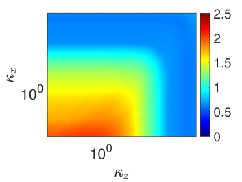
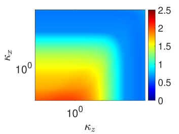
We will compute on an grid of space and temporal frequencies. The spatial frequencies (wavenumbers) and are both defined on a log-spaced grid of points in the interval . This grid is denoted . The temporal frequency is defined on a grid , where is the wave speed, i.e., speed of the moving base flow (see [12] for details). Wave speeds are chosen as resulting in points in the temporal frequency grid. Additionally, we will fix and for all computations and use MATLAB’s parfor command to loop over temporal frequencies.
4.3 Discussion
We can see in figure 1 that values are qualitatively and quantitatively similar (within ) to the upper-bounds of obtained from Algorithm 1 in [13]. In fact, values are “identical” to the lower-bound values of (not shown here), i.e., values match up to . Thus, the algorithms converge to the optimal solutions obtained from our method.
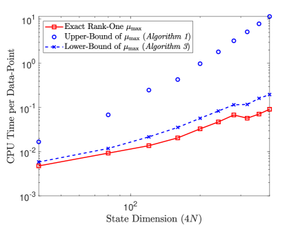
Furthermore, computing is relatively fast as compared to obtaining its bounds (see figure 2). Each point on the plot in figure 2 represents the average222The CPU times are averaged over data-points. We used an ASUS ROG M15 laptop with Intel 2.6 GHz i7-10750H CPU with 6 cores, 16 GB RAM, and an RTX 2070 Max-Q GPU for run time computations. CPU time for a single data-point at each of the state dimensions. All computational times include CPU time for SVD of to obtain a rank-one approximation. From the plot in figure 2, the upper-bound and lower-bound solutions have a time complexity of and , respectively. Meanwhile, computing from our method has a time complexity of .
5 Conclusion
This work presents an exact solution of SSV for rank-one complex matrices with repeated, complex full-block uncertainties. The solution obtained from this method generalizes previous exact solutions for the repeated complex scalar and/or non-repeated complex full-block uncertainties [2, 1]. We illustrated the proposed method on a turbulent channel flow model. In future work, we would like to explore similar arguments to the ones presented here for rank-one complex matrices to compute SSV for general (not necessarily rank-one) complex matrices, especially when .
6 Acknowledgements
This material is based upon work supported by the ARO under grant number W911NF-20-1-0156. MSH acknowledges support from the AFOSR under award number FA 9550-19-1-0034, the NSF under grant number CBET-1943988 and ONR under award number N000140-22-1-2029.
References
- [1] P. M. Young, “The rank one mixed problem and ‘kharitonov-type’ analysis,” Automatica, vol. 30, no. 12, pp. 1899–1911, 1994.
- [2] J. Chen, M. K. Fan, and C. N. Nett, “Structured singular values and stability analysis of uncertain polynomials, part 1: the generalized ,” Systems & control letters, vol. 23, no. 1, pp. 53–65, 1994.
- [3] ——, “Structured singular values and stability analysis of uncertain polynomials, part 2: a missing link,” Systems & control letters, vol. 23, no. 2, pp. 97–109, 1994.
- [4] A. Packard and J. Doyle, “The complex structured singular value,” Automatica, vol. 29, no. 1, pp. 71–109, 1993.
- [5] M. K. Fan, J. C. Doyle, and A. L. Tits, “Robustness in the presence of parametric uncertainty and unmodeled dynamics,” in Advances in Computing and Control. Springer, 2006, pp. 363–367.
- [6] J. Von Neumann, “Some matrix-inequalities and metrization of matric-space. tomsk univ. rev. 1, 286–300 (1937). reprinted in collected works,” 1962.
- [7] C. Liu and D. F. Gayme, “Structured input–output analysis of transitional wall-bounded flows,” Journal of Fluid Mechanics, vol. 927, Sept. 2021.
- [8] C. Liu, P. C. Colm-cille, and D. F. Gayme, “Structured input–output analysis of stably stratified plane couette flow,” Journal of Fluid Mechanics, vol. 948, p. A10, 2022.
- [9] D. Bhattacharjee, T. Mushtaq, P. J. Seiler, and M. Hemati, “Structured input-output analysis of compressible plane Couette flow,” AIAA Paper 2023-1984, 2023.
- [10] T. Mushtaq, D. Bhattacharjee, P. J. Seiler, and M. Hemati, “Structured input-output tools for modal analysis of a transitional channel flow,” AIAA Paper 2023-1805, 2023.
- [11] T. Mushtaq, M. Luhar, and M. Hemati, “Structured input-output analysis of turbulent flows over riblets,” AIAA Paper 2023-3446, 2023.
- [12] B. McKeon, “The engine behind (wall) turbulence: perspectives on scale interactions,” Journal of Fluid Mechanics, vol. 817, p. P1, 2017.
- [13] T. Mushtaq, D. Bhattacharjee, P. Seiler, and M. S. Hemati, “Structured singular value of a repeated complex full block uncertainty,” Submitted to International Journal of Robust and Nonlinear Control for Review, 2023.
- [14] L. Qiu and E. Davison, “A simple procedure for the exact stability robustness computation of polynomials with affine coefficient perturbations,” Systems & control letters, vol. 13, no. 5, pp. 413–420, 1989.
- [15] S. Boyd and L. Vandenberghe, Convex Optimization. Cambridge University Press, 2004.