Benchmark computations of dynamic poroelasticity

Abstract

We present benchmark computations of dynamic poroelasticity modeling fluid flow in deformable porous media by a coupled hyperbolic-parabolic system of partial differential equations. A challenging benchmark setting and goal quantities of physical interest for this problem are proposed. Computations performed by space-time finite element approximations with continuous and discontinuous discretizations of the time variable are summarized. By this work we intend to stimulate comparative studies by other research groups for the evaluation of dynamic poroelasticity solver regarding the accuracy of discretization techniques, the efficiency and robustness of iterative methods for the linear systems and the arrangement of the model equations in terms of their variables (two-field or multi-field formulations).

1 Introduction and mathematical model

In this work we present benchmark computations for families of space-time finite element approximations (cf., e.g., [2, 5, 13, 14, 18, 17]) to the coupled hyperbolic-parabolic problem

$$\rho\partial_{t}^{2}\boldsymbol{u}-\nabla\cdot(\boldsymbol{C}\boldsymbol{\varepsilon}(\boldsymbol{u}))+\alpha\boldsymbol{\nabla}p =\rho\boldsymbol{f}\,,\qquad c_{0}\partial_{t}p+\alpha\nabla\cdot\partial_{t}\boldsymbol{u}-\nabla\cdot(\boldsymbol{K}\nabla p) =g\,, \quad\text{in }\;\Omega\times(0,T]\,,$$ (1.1a)

$$\boldsymbol{u}(0)=\boldsymbol{u}_{0}\,,\quad\partial_{t}\boldsymbol{u}(0) =\boldsymbol{u}_{1}\,, p(0) =p_{0}\,, \quad\text{in }\;\Omega\times\{0\}\,,$$ (1.1b)

$$\boldsymbol{u}=\boldsymbol{u}_{D}\,,\quad\text{on }\;\Gamma_{\boldsymbol{u}}^{D}\times( 0,T]\,, \quad-(\boldsymbol{C}\boldsymbol{\varepsilon}(\boldsymbol{u})-\alpha p\boldsymbol{E})\boldsymbol{n} =\boldsymbol{t}_{N}\,, \quad\text{on }\;\Gamma_{\boldsymbol{u}}^{{N}}\times(0,T]\,,$$ (1.1c)

$$p=p_{D}\,,\quad\text{on }\;\Gamma_{p}^{{D}}\times( 0,T]\,, -\boldsymbol{K}\nabla p\cdot\boldsymbol{n} =p_{N}\,, \quad\text{on }\;\Gamma_{p}^{{N}}\times(0,T]\,.$$ (1.1d)

Componentwise or directional boundary conditions for $\boldsymbol{u}$, given by

$$\boldsymbol{u}\cdot\boldsymbol{n}=0\qquad\text{and}\qquad(\boldsymbol{\sigma}(\boldsymbol{u})\boldsymbol{n})\cdot\boldsymbol{t}_{i}=0\,,\quad\text{for}\;\;i=1,\ldots,d-1\,,\quad\text{on}\;\;\Gamma^{d}_{\boldsymbol{u}}\times(0,T]\,,$$ (1.2)

are applied further for the sake of physical realism; cf. Fig. 4.1. In (1.1), $\Omega\subset\mathbb{R}^{d}$, with $d\in\{2,3\}$, is an open bounded Lipschitz domain with outer unit normal vector $\boldsymbol{n}$ to the boundary $\partial\Omega$ and $T>0$ is the final time point. For (1.1c) and (1.1d), we let $\partial\Omega={\Gamma_{\boldsymbol{u}}^{D}}\cup{\Gamma_{\boldsymbol{u}}^{N}}$ and $\partial\Omega={\Gamma_{p}^{D}}\cup{\Gamma_{p}^{N}}$ with closed portions $\Gamma_{\boldsymbol{u}}^{D}$ and $\Gamma_{p}^{D}$ of non-zero measure. In (1.2), we denote by $\boldsymbol{t}_{i}$, for $i=1,\ldots,d-1$, the unit basis vectors of the tangent space at $\boldsymbol{x}\in\Gamma^{d}_{\boldsymbol{u}}$. For (1.2), the decomposition $\partial\Omega={\Gamma_{\boldsymbol{u}}^{N}}\cup\Gamma^{d}_{\boldsymbol{u}}$ of the boundary of a L-shaped domain $\Omega$ that is used for our computations is illustrated in Fig. 4.1. The unknowns in (1.1) are the vector-valued variable $\boldsymbol{u}$ and the scalar function $p$. The quantity $\boldsymbol{\varepsilon}(\boldsymbol{u}):=(\nabla\boldsymbol{u}+(\nabla\boldsymbol{u})^{\top})/2$ denotes the symmetrized gradient and $\boldsymbol{E}\in\mathbb{R}^{d,d}$ is the identity matrix. For brevity, the positive quantities $\rho>0$, $\alpha>0$ and $c_{0}>0$ as well as the tensors $\boldsymbol{C}$ and $\boldsymbol{K}$ are assumed to be constant in space and time. The tensors $\boldsymbol{C}$ and $\boldsymbol{K}$ are supposed to be symmetric and positive definite,

$$\exists k_{0}>0\;\forall\boldsymbol{\xi}=\boldsymbol{\xi}^{\top}\in\mathbb{R}^{d,d}:\;\sum_{i,j,k,l=1}^{d}\xi_{ij}C_{ijkl}\xi_{kl}\geq k_{0}\sum_{j,k=1}^{d}|\xi_{jk}|^{2}\,,\quad\exists k_{1}>0\;\forall\boldsymbol{\xi}\in\mathbb{R}^{d}:\;\sum_{i,j,=1}^{d}\xi_{i}K_{ij}\xi_{j}\geq k_{1}\sum_{i=1}^{d}|\xi_{i}|^{2}\,.$$

Under these assumptions, well-posedness of (1.1) is ensured. This has been shown by different mathematical techniques and for several combinations of boundary conditions in, e.g., [15, 22, 21]. In [2], well-posedness of a fully discrete space-time finite element approximation is proved for the boundary conditions in (1.2), applied to the L-shaped domain $\Omega$ of Fig. 4.1.

Important and classical applications of the system (1.1) arise in poroelasticity and thermoelasticity; cf., e.g., [7, 8, 9] and [12, 15, 19]. Recently, generalizations of the system (1.1) to soft materials have strongly attracted researchers’ interest in biomedicine; cf., e.g., [10, 11] and the references therein. In neurophysiology, such generalizations are used to model, simulate and elucidate circulatory diseases, such as ischaemic stroke, or also Alzheimer’s disease. In poroelasticity, Eqs. (1.1) are referred to as the dynamic Biot model. The system (1.1) is used to describe flow of a slightly compressible viscous fluid through a deformable porous matrix. The small deformations of the matrix are described by the Navier equations of linear elasticity, and the diffusive fluid flow is described by Duhamel’s equation. The unknowns are the effective solid phase displacement $\boldsymbol{u}$ and the effective fluid pressure $p$. The quantity $\boldsymbol{\varepsilon}(\boldsymbol{u})$ is the strain tensor. Further, $\rho$ is the effective mass density, $\boldsymbol{C}$ is Gassmann’s fourth order effective elasticity tensor, $\alpha$ is Biot’s pressure-storage coupling tensor, $c_{0}$ is the specific storage coefficient and $\boldsymbol{K}$ is the permeability. In thermoelasticity, $p$ denotes the temperature, $c_{0}$ is the specific heat of the medium, and $\boldsymbol{K}$ is the conductivity. Then, the quantity $\alpha\nabla p$ arises from the thermal stress in the structure, and $\alpha\nabla\cdot\partial_{t}\boldsymbol{u}$ models the internal heating due to the dilation rate.

2 Space-time finite element approximation

We rewrite (1.1) as a first-order in time system by introducing the new variable $\boldsymbol{v}:=\partial_{t}\boldsymbol{u}$. Then, we recover (1.1a) as

$$\partial_{t}\boldsymbol{u}-\boldsymbol{v}=\boldsymbol{0}\,,\quad\rho\partial_{t}\boldsymbol{v}-\nabla\cdot(\boldsymbol{C}\boldsymbol{\varepsilon}(\boldsymbol{u}))+\alpha\boldsymbol{\nabla}p=\rho\boldsymbol{f}\,,\qquad c_{0}\partial_{t}p+\alpha\nabla\cdot\boldsymbol{v}-\nabla\cdot(\boldsymbol{K}\boldsymbol{\nabla}p)=g\,,$$ (2.1)

along with the initial and boundary conditions (1.1b) to (1.1d). We benchmark the application of space-time finite element methods to (2.1), with continuous and discontinuous Galerkin methods for the discretization of the time variable and inf-sup stable pairs of finite elements for the approximation of the space variables. To introduce the scheme we need notation.

For the time discretization, we decompose $I:=(0,T]$ into $N$ subintervals $I_{n}=(t_{n-1},t_{n}]$, $n=1,\ldots,N$, where $0=t_{0}<t_{1}<\cdots<t_{N-1}<t_{N}=T$ such that $I=\bigcup_{n=1}^{N}I_{n}$. We put $\tau:=\max_{n=1,\ldots,N}\tau_{n}$ with $\tau_{n}=t_{n}-t_{n-1}$. The set $\mathcal{M}_{\tau}:=\{I_{1},\ldots,I_{N}\}$ of time intervals is called the time mesh. For a Banach space $B$, any $k\in\mathbb{N}_{0}$ and $\mathbb{P}_{k}(I_{n};B):=\big{\{}w_{\tau}\,:\,I_{n}\to B\,,\;w_{\tau}(t)=\sum_{j=0}^{k}W^{j}t^{j}\;\forall t\in I_{n}\,,\;W^{j}\in B\;\forall j\big{\}}$ we define the space of piecewise polynomial functions in time with values in $B$ by

$$Y_{\tau}^{k}(B):=\left\{w_{\tau}:\overline{I}\rightarrow B\mid w_{\tau}{}_{|I_{n}}\in\mathbb{P}_{k}(I_{n};B)\;\forall I_{n}\in\mathcal{M}_{\tau},\,w_{\tau}(0)\in B\right\}\subset L^{2}(I;B)\,.$$ (2.2)

For any function $w:\overline{I}\to B$ that is piecewise sufficiently smooth with respect to the time mesh $\mathcal{M}_{\tau}$, for instance for $w\in Y^{k}_{\tau}(B)$, we define the right-hand sided and left-hand sided limit at a mesh point $t_{n}$ by $w^{+}(t_{n}):=\lim_{t\to t_{n}+0}w(t)$ for $n<N$ and $w^{-}(t_{n}):=\lim_{t\to t_{n}-0}w(t)$ for $n>0$. Further, for a Banach space $B$ and any $k\in\mathbb{N}$ we define

$$X_{\tau}^{k}(B):=\left\{w_{\tau}\in C(\overline{I};B)\mid w_{\tau}{}_{|I_{n}}\in\mathbb{P}_{k}(I_{n};B)\;\forall I_{n}\in\mathcal{M}_{\tau}\right\}\,.$$ (2.3)

For time integration, it is natural to use the right-sided $(k+1)$-point Gauss–Radau (GR) quadrature formula in a discontinuous Galerkin approach and the $(k+1)$-point Gauss–Lobatto (GL) quadrature formula in a continuous one. On $I_{n}$, they read as

$$Q_{n}^{\text{q}}(w):=\frac{\tau_{n}}{2}\sum_{\mu=1}^{k+1}\hat{\omega}_{\mu}^{\operatorname{q}}w(t_{n,\mu}^{\operatorname{q}})\approx\int_{I_{n}}w(t)\,\mathrm{d}t\,,\quad\text{for}\;\text{q}\in\{\operatorname{GR},\operatorname{GL}\}\,,$$ (2.4)

where $t_{n,\mu}^{\operatorname{q}}=T_{n}(\hat{t}_{\mu}^{\operatorname{q}})$, for $\mu=1,\ldots,k+1$, are the quadrature points on $I_{n}$ and $\hat{\omega}_{\mu}^{\operatorname{q}}$ the corresponding weights of the respective quadrature formula. Here, $T_{n}(\hat{t}):=(t_{n-1}+t_{n})/2+(\tau_{n}/2)\hat{t}$ is the affine transformation from $\hat{I}=[-1,1]$ to $I_{n}$ and $\hat{t}_{\mu}^{\operatorname{q}}$ are the quadrature points on $\hat{I}$. Formula (2.4) is exact for all $w\in\mathbb{P}_{2k}(I_{n};\mathbb{R})$ if $\text{q}=\operatorname{GR}$, and for all $w\in\mathbb{P}_{2k-1}(I_{n};\mathbb{R})$ if $\text{q}=\operatorname{GL}$ .

For the space discretization, let $\mathcal{T}_{h}=\{K\}$ be the quasi-uniform decomposition of $\Omega$ into (open) quadrilaterals or hexahedrals, with mesh size $h>0$. These element types are chosen for our implementation (cf. Sec. 3 and 4) that uses the deal.II library [4]. The finite element spaces used for approximating the unknowns $\boldsymbol{u}$, $\boldsymbol{v}$ and $p$ of (2.1) in space are of the form

$$\boldsymbol{V}_{h} :=\{\boldsymbol{v}_{h}\in C(\overline{\Omega})^{d}\mid\boldsymbol{v}_{h}{}_{|K}\in{\boldsymbol{V}(K)}\;\;\text{for all}\;K\in\mathcal{T}_{h}\}\,,$$ (2.5a)

$$Q_{h} :=\{\boldsymbol{q}_{h}\in L^{2}(\Omega)\mid\boldsymbol{q}_{h}{}_{|K}\in{Q(K)}\;\;\text{for all}\;K\in\mathcal{T}_{h}\}\,.$$ (2.5b)

For the local spaces $\boldsymbol{V}(K)$ and $Q(K)$ we employ mapped versions of the inf-sup stable pair $\mathbb{Q}_{r}^{d}/\mathbb{P}_{r-1}^{\operatorname{disc}}$, for $r\geq 2$, of finite element spaces; cf. [16]. The pair $\mathbb{Q}_{r}^{d}/\mathbb{P}_{r-1}^{\operatorname{disc}}$ with a discontinuous approximation of $p$ in the broken polynomial space $Q_{h}$ has proved excellent accuracy and stability properties for higher-order approximations of mixed (or saddle point) systems like the Navier–Stokes equations and the applicability of geometric multigrid preconditioner for the algebraic systems; cf., e.g., [1, 3].

For $\boldsymbol{w}_{h},\boldsymbol{\chi}_{h}\in\boldsymbol{V}_{h}$ and $q_{h},\psi_{h}\in Q_{h}$ we define the bilinear forms

$$A_{\gamma}(\boldsymbol{w}_{h},\boldsymbol{\chi}_{h}) :=\langle\boldsymbol{C}\boldsymbol{\varepsilon}(\boldsymbol{w}_{h}),\boldsymbol{\varepsilon}(\boldsymbol{\chi}_{h})\rangle-\langle\boldsymbol{C}\boldsymbol{\varepsilon}(\boldsymbol{w}_{h})\boldsymbol{n},\boldsymbol{\chi}_{h}\rangle_{\Gamma^{D}_{\boldsymbol{u}}}+a_{\gamma}(\boldsymbol{w}_{h},\boldsymbol{\chi}_{h})\,,$$ (2.6a)

$$C(\boldsymbol{\chi}_{h},q_{h}) :=-\alpha\langle\nabla\cdot\boldsymbol{\chi}_{h},q_{h}\rangle+\alpha\langle\boldsymbol{\chi}_{h}\cdot\boldsymbol{n},q_{h}\rangle_{\Gamma^{D}_{\boldsymbol{u}}}\,,$$ (2.6b)

$$B_{\gamma}(q_{h},\psi_{h}) :=\begin{array}[t]{@{}l}\displaystyle\sum_{K\in\mathcal{T}_{l}}\langle\boldsymbol{K}\nabla q_{h},\nabla\psi_{h}\rangle_{K}-\sum_{F\in\mathcal{F}_{h}}\big{(}\langle\{\mskip-5.0mu\{\boldsymbol{K}\nabla q_{h}\}\mskip-5.0mu\}\cdot\boldsymbol{n},\lsem\psi_{h}\rsem\rangle_{F}+\langle\lsem q_{h}\rsem,\{\mskip-5.0mu\{\boldsymbol{K}\nabla\psi_{h}\}\mskip-5.0mu\}\cdot\boldsymbol{n}\rangle_{F}\big{)}+b_{\gamma}(q_{h},\psi_{h})\,,\end{array}$$ (2.6d)

where $a_{\gamma}(\cdot,\cdot)$ in (2.6a) is given by $a_{\gamma}(\boldsymbol{w},\boldsymbol{\chi}_{h}):=-\langle\boldsymbol{w},\boldsymbol{C}\boldsymbol{\varepsilon}(\boldsymbol{\chi}_{h})\boldsymbol{n}\rangle_{\Gamma^{D}_{\boldsymbol{u}}}+{\gamma_{a}}{h_{F}^{-1}}\langle\boldsymbol{w},\boldsymbol{\chi}_{h}\rangle_{\Gamma^{D}_{\boldsymbol{u}}}$, for $\boldsymbol{w}\in\boldsymbol{H}^{1/2}(\Gamma^{D}_{\boldsymbol{u}})$, and $b_{\gamma}(\cdot,\cdot)$ in (2.6d) is defined by $b_{\gamma}(q_{h},\psi_{h})=\sum_{F\in\mathcal{F}_{h}}{\gamma_{b}}{h_{F}^{-1}}\langle\lsem q_{h}\rsem,\lsem\psi_{h}\rsem\rangle_{F}$. The form $B_{\gamma}$ yields a symmetric interior penalty discontinuous Galerkin discretization of the scalar variable $p$; cf., e.g., [20, Sec. 4.2]. As usual, the average $\{\mskip-5.0mu\{\cdot\}\mskip-5.0mu\}$ and jump $\lsem\cdot\rsem$ for a function $w$ of a broken space on an interior face $F$ between two elements $K^{+}$ and $K^{-}$, such that $F=\partial K^{+}\cap\partial K^{-}$, are defined by $\{\mskip-5.0mu\{w\}\mskip-5.0mu\}:=\frac{1}{2}(w^{+}+w^{-})$ and $\lsem w\rsem:=w^{+}-w^{-}$. For boundary faces $F\subset\partial K\cap\partial\Omega$, we set $\{\mskip-5.0mu\{w\}\mskip-5.0mu\}:=w_{|K}$ and $\lsem w\rsem:=w_{|K}$. The set of all faces (interior and boundary faces) on $\mathcal{T}_{h}$ is denoted by $\mathcal{F}_{h}$. In (2.6d), the parameter $\gamma_{b}$ in $b_{\gamma}$ has to be chosen sufficiently large, such that the discrete coercivity of $B_{\gamma}$ on $Q_{h}$ is preserved. The local length $h_{F}$ is chosen as $h_{F}=\{\mskip-5.0mu\{h_{F}\}\mskip-5.0mu\}:=\frac{1}{2}(|K^{+}|_{d}+|K^{-}|_{d})$ with Hausdorff measure $|\cdot|_{d}$; cf. [20, p. 125]. For boundary faces we set $h_{F}:=|K|_{d}$. In $a_{\gamma}(\cdot,\cdot)$ , the quantity $\gamma_{a}$ is the algorithmic parameter of the stabilization (or penalization) term in the Nitsche formulation [6, 2] for incorporating Dirichlet boundary conditions in weak form which is applied here. To ensure well-posedness of the discrete systems, the parameter $\gamma_{a}$ has to be chosen sufficiently large as well; cf. [2, Appendix]. Based on our numerical experiments we choose the algorithmic parameter $\gamma_{a}$ and $\gamma_{b}$ as $\gamma_{a}=5\cdot 10^{4}\cdot r\cdot(r+1)$ and $\gamma_{b}=\frac{1}{2}\cdot r\cdot(r-1)$, where $r$ is the polynomial degree of $\boldsymbol{V}_{h}$ in (2.5a). Finally, for $\boldsymbol{f}\in\boldsymbol{H}^{-1}(\Omega)$, $\boldsymbol{u}_{D}\in\boldsymbol{H}^{1/2}(\Gamma^{D}_{\boldsymbol{u}})$, $\boldsymbol{t}_{N}\in\boldsymbol{H}^{-1/2}(\Gamma^{N}_{\boldsymbol{u}})$ and $g\in H^{-1}(\Omega)$, $p_{D}\in H^{1/2}(\Gamma^{D}_{p})$, $p_{N}\in H^{-1/2}(\Gamma^{N}_{p})$ we put

$$F_{\gamma}(\boldsymbol{\chi}_{h}):=\langle\boldsymbol{f},\boldsymbol{\chi}_{h}\rangle-\langle\boldsymbol{t}_{N},\boldsymbol{\chi}_{h}\rangle_{\Gamma^{N}_{\boldsymbol{u}}}+a_{\gamma}(\boldsymbol{u}_{D},\boldsymbol{\chi}_{h})\,,\qquad G_{\gamma}(\psi_{h}):=\langle g,\psi_{h}\rangle-\sum_{F\in\mathcal{F}_{h}^{D,\boldsymbol{u}}}\alpha\langle\boldsymbol{v}_{D}\cdot\boldsymbol{n},\psi_{h}\rangle_{F}$$

$$-\sum_{F\in\mathcal{F}_{h}^{D,p}}\langle p_{D},\{\mskip-5.0mu\{\boldsymbol{K}\nabla\psi_{h}\}\mskip-5.0mu\}\cdot\boldsymbol{n}\rangle_{F}+\sum_{F\in\mathcal{F}_{h}^{D,p}}{\gamma_{b}}{h_{F}^{-1}}\langle p_{D},\lsem\psi_{h}\rsem\rangle_{F}-\sum_{F\subset\mathcal{F}_{h}^{N,p}}\langle p_{N},\lsem\psi_{h}\rsem\rangle_{F}\,.$$

Here, we denote by $\mathcal{F}_{h}^{D,p}\subset\mathcal{F}_{h}$ and $\mathcal{F}_{h}^{N,p}\subset\mathcal{F}_{h}$ the set of all element faces on the boundary parts $\Gamma_{p}^{D}$ and $\Gamma_{p}^{N}$, respectively; cf. (1.1). The second of the terms on the right-hand side of $G_{\gamma}(\cdot,\cdot)$ with $\boldsymbol{v}_{D}=\partial_{t}\boldsymbol{u}_{D}$, is added to ensure consistency of the form $C(\cdot,\cdot)$ in (2.6b); cf. [2, p. 8] for details.

We use a temporal test basis that is supported on the subintervals $I_{n}$. Then, a time marching process is obtained. In that, we assume that the trajectories $\boldsymbol{u}_{\tau,h}$, $\boldsymbol{v}_{\tau,h}$ and $p_{\tau,h}$ have been computed before for all $t\in[0,t_{n-1}]$, starting with approximations $\boldsymbol{u}_{\tau,h}(t_{0}):=\boldsymbol{u}_{0,h}$, $\boldsymbol{v}_{\tau,h}(t_{0}):=\boldsymbol{u}_{1,h}$ and $p_{\tau,h}(t_{0}):=p_{0,h}$ of the initial values $\boldsymbol{u}_{0}$, $\boldsymbol{u}_{1}$ and $p_{0}$. Then, we consider solving the following local problems on $I_{n}$ of the discontinuous (dG($k$)) and continuous (cG($k$)) Galerkin approximation in time; cf. [2, 5].

Problem 2.1 ($I_{n}$-problem for dG($k$))

Let $k\in\mathbb{N}_{0}$. For given $\boldsymbol{u}_{h}^{n-1}:=\boldsymbol{u}_{\tau,h}(t_{n-1})\in\boldsymbol{V}_{h}$, $\boldsymbol{v}_{h}^{n-1}:=\boldsymbol{v}_{\tau,h}(t_{n-1})\in\boldsymbol{V}_{h}$, and $p_{h}^{n-1}:=p_{\tau,h}(t_{n-1})\in Q_{h}$ with $\boldsymbol{u}_{\tau,h}(t_{0}):=\boldsymbol{u}_{0,h}$, $\boldsymbol{v}_{\tau,h}(t_{0}):=\boldsymbol{u}_{1,h}$ and $p_{\tau,h}(t_{0}):=p_{0,h}$, find $(\boldsymbol{u}_{\tau,h},\boldsymbol{v}_{\tau,h},p_{\tau,h})\in\mathbb{P}_{k}(I_{n};\boldsymbol{V}_{h})\times\mathbb{P}_{k}(I_{n};\boldsymbol{V}_{h})\times\mathbb{P}_{k}(I_{n};Q_{h})$ such that for all $(\boldsymbol{\phi}_{\tau,h},\boldsymbol{\chi}_{\tau,h},\psi_{\tau,h})\in\mathbb{P}_{k}(I_{n};\boldsymbol{V}_{h})\times\mathbb{P}_{k}(I_{n};\boldsymbol{V}_{h})\times\mathbb{P}_{k}(I_{n};Q_{h})$,

$$\begin{aligned} &Q_{n}^{\operatorname{GR}}\big{(}\langle\partial_{t}\boldsymbol{u}_{\tau,h},\boldsymbol{\phi}_{\tau,h}\rangle-\langle\boldsymbol{v}_{\tau,h},\boldsymbol{\phi}_{\tau,h}\rangle\big{)}+\langle\boldsymbol{u}^{+}_{\tau,h}(t_{n-1}),\boldsymbol{\phi}_{\tau,h}^{+}(t_{n-1})\rangle=\langle\boldsymbol{u}_{h}^{n-1},\boldsymbol{\phi}_{\tau,h}^{+}(t_{n-1})\rangle\,,\\[2.15277pt] \end{aligned}$$ (2.8a)

$$\begin{aligned} &Q_{n}^{\operatorname{GR}}\Big{(}\langle\rho\partial_{t}\boldsymbol{v}_{\tau,h},\boldsymbol{\chi}_{\tau,h}\rangle+A_{\gamma}(\boldsymbol{u}_{\tau,h},\boldsymbol{\chi}_{\tau,h})+C(\boldsymbol{\chi}_{\tau,h},p_{\tau,h})\Big{)}+\langle\rho\boldsymbol{v}^{+}_{\tau,h}(t_{n-1}),\boldsymbol{\chi}_{\tau,h}^{+}(t_{n-1})\rangle\\[2.15277pt] &\quad=Q_{n}^{\operatorname{GR}}\Big{(}F_{\gamma}(\boldsymbol{\chi}_{\tau,h})\Big{)}+\langle\rho\boldsymbol{v}_{h}^{n-1},\chi_{\tau,h}^{+}(t_{n-1})\rangle\,,\\[2.15277pt] \end{aligned}$$ (2.8b)

$$\begin{aligned} &Q_{n}^{\operatorname{GR}}\Big{(}\langle c_{0}\partial_{t}p_{\tau,h},\psi_{\tau,h}\rangle-C(\boldsymbol{v}_{\tau,h},\psi_{\tau,h})+B_{\gamma}(p_{\tau,h},\psi_{\tau,h})\Big{)}+\langle c_{0}p^{+}_{\tau,h}(t_{n-1}),\psi_{\tau,h}^{+}(t_{n-1})\rangle\\[2.15277pt] &\quad=Q_{n}^{\operatorname{GR}}\Big{(}G_{\gamma}(\psi_{\tau,h})\Big{)}+\langle c_{0}p_{h}^{n-1},\psi_{\tau,h}^{+}(t_{n-1})\rangle\,.\end{aligned}$$ (2.8c)

The trajectories defined by Problem 2.1, for $n=1,\ldots,N$, satisfy that $\boldsymbol{u}_{\tau,h},\boldsymbol{v}_{\tau,h}\in Y_{\tau}^{k}(\boldsymbol{V}_{h})$ and $p_{\tau,h}\in Y_{\tau}^{k}(Q_{h})$; cf. (2.2). Well-posedness of Problem 2.1 is ensured; cf. [2, Lem. 3.2].

Problem 2.2 ($I_{n}$-problem for cG($k$))

Let $k\in\mathbb{N}$. For given $\boldsymbol{u}_{h}^{n-1}:=\boldsymbol{u}_{\tau,h}(t_{n-1})\in\boldsymbol{V}_{h}$, $\boldsymbol{v}_{h}^{n-1}:=\boldsymbol{v}_{\tau,h}(t_{n-1})\in\boldsymbol{V}_{h}$, and $p_{h}^{n-1}:=p_{\tau,h}(t_{n-1})\in Q_{h}$ with $\boldsymbol{u}_{\tau,h}(t_{0}):=\boldsymbol{u}_{0,h}$, $\boldsymbol{v}_{\tau,h}(t_{0}):=\boldsymbol{u}_{1,h}$ and $p_{\tau,h}(t_{0}):=p_{0,h}$, find $(\boldsymbol{u}_{\tau,h},\boldsymbol{v}_{\tau,h},p_{\tau,h})\in\mathbb{P}_{k}(I_{n};\boldsymbol{V}_{h})\times\mathbb{P}_{k}(I_{n};\boldsymbol{V}_{h})\times\mathbb{P}_{k}(I_{n};Q_{h})$ such that

$$\boldsymbol{u}_{\tau,h}^{+}(t_{n-1})=\boldsymbol{u}_{h}^{n-1}\,,\quad\boldsymbol{v}_{\tau,h}^{+}(t_{n-1})=\boldsymbol{v}_{h}^{n-1}\quad\text{and}\quad p_{\tau,h}^{+}(t_{n-1})=p_{h}^{n-1}$$ (2.9)

and, for all $(\boldsymbol{\phi}_{\tau,h},\boldsymbol{\chi}_{\tau,h},\psi_{\tau,h})\in\mathbb{P}_{k-1}(I_{n};\boldsymbol{V}_{h})\times\mathbb{P}_{k-1}(I_{n};\boldsymbol{V}_{h})\times\mathbb{P}_{k-1}(I_{n};Q_{h})$,

$$\begin{aligned} &Q_{n}^{\operatorname{GL}}\big{(}\langle\partial_{t}\boldsymbol{u}_{\tau,h},\boldsymbol{\phi}_{\tau,h}\rangle-\langle\boldsymbol{v}_{\tau,h},\boldsymbol{\phi}_{\tau,h}\rangle\big{)}=0\,,\\[2.15277pt] \end{aligned}$$ (2.10a)

$$\begin{aligned} &Q_{n}^{\operatorname{GL}}\Big{(}\langle\rho\partial_{t}\boldsymbol{v}_{\tau,h},\boldsymbol{\chi}_{\tau,h}\rangle+A_{\gamma}(\boldsymbol{u}_{\tau,h},\boldsymbol{\chi}_{\tau,h})+C(\boldsymbol{\chi}_{\tau,h},p_{\tau,h})\Big{)}=Q_{n}^{\operatorname{GL}}\Big{(}F_{\gamma}(\boldsymbol{\chi}_{\tau,h})\Big{)}\,,\\[2.15277pt] \end{aligned}$$ (2.10b)

$$\begin{aligned} &Q_{n}^{\operatorname{GL}}\Big{(}\langle c_{0}\partial_{t}p_{\tau,h},\psi_{\tau,h}\rangle-C(\boldsymbol{v}_{\tau,h},\psi_{\tau,h})+B_{\gamma}(p_{\tau,h},\psi_{\tau,h})\Big{)}=Q_{n}^{\operatorname{GL}}\Big{(}G_{\gamma}(\psi_{\tau,h})\Big{)}\,.\end{aligned}$$ (2.10c)

The trajectories defined by Problem 2.2, for $n=1,\ldots,N$, satisfy that $\boldsymbol{u}_{\tau,h},\boldsymbol{v}_{\tau,h}\in X_{\tau}^{k}(\boldsymbol{V}_{h})$ and $p_{\tau,h}\in X_{\tau}^{k}(Q_{h})$; cf. (2.3). Well-posedness of Problem 2.2 can be shown following the arguments [2, Lem. 3.2]. Precisely, the cG($k$) scheme of Problem 2.2 represents a Galerkin–Petrov approach since trial and test spaces differ from each other.

Remark 2.3 (Algebraic solver)

Problem 2.1 and 2.2 lead to large linear algebraic systems with complex block structure, in particular for larger values of the piecewise polynomial order in time $k$. This puts a facet of complexity on their solution, in particular if three space dimensions are involved. To solve such type of block systems, we use GMRES iterations that are preconditioned by a V-cycle geometric multigrid method based on a local Vanka smoother; cf. [1, 2] for details.

3 Numerical convergence test

$\tau$ $h$ $\|\nabla(\boldsymbol{u}-\boldsymbol{u}_{\tau,h})\|_{L^{2}(\boldsymbol{L}^{2})}$ EOC $\|\boldsymbol{v}-\boldsymbol{v}_{\tau,h}\|_{L^{2}(\boldsymbol{L}^{2})}$ EOC $\|p-p_{\tau,h}\|_{L^{2}(L^{2})}$ EOC $\tau_{0}/2^{0}$ $h_{0}/2^{0}$ 1.2138632264e-02 – 3.4963867086e-02 – 2.0325417612e-03 – $\tau_{0}/2^{1}$ $h_{0}/2^{1}$ 1.4699245816e-03 3.05 3.9349862997e-03 3.15 2.3314471675e-04 3.12 $\tau_{0}/2^{2}$ $h_{0}/2^{2}$ 1.8238666739e-04 3.01 4.8313770355e-04 3.03 2.8891798035e-05 3.01 $\tau_{0}/2^{3}$ $h_{0}/2^{3}$ 2.2707201873e-05 3.01 6.0087160884e-05 3.01 3.6067034147e-06 3.00 $\tau_{0}/2^{4}$ $h_{0}/2^{4}$ 2.8305414233e-06 3.00 7.4900993341e-06 3.00 4.5021336614e-07 3.00

Table 3.1: $L^{2}(L^{2})$ errors and experimental orders of convergence (EOC) for (3.1) with spatial degree $r=4$ for the spaces $\mathbb{Q}_{r}^{2}/\mathbb{P}_{r-1}^{\text{disc}}$ and temporal degree $k=2$ for the dG($k$) scheme of Problem 2.1.

$\tau$ $h$ $\|\nabla(\boldsymbol{u}-\boldsymbol{u}_{\tau,h})\|_{L^{2}(\boldsymbol{L}^{2})}$ EOC $\|\boldsymbol{v}-\boldsymbol{v}_{\tau,h}\|_{L^{2}(\boldsymbol{L}^{2})}$ EOC $\|p-p_{\tau,h}\|_{L^{2}(L^{2})}$ EOC $\tau_{0}/2^{0}$ $h_{0}/2^{0}$ 9.8743046869e-04 – 3.5668679054e-03 – 4.3639594011e-04 – $\tau_{0}/2^{1}$ $h_{0}/2^{1}$ 5.9913786816e-05 4.04 1.5360551492e-04 4.54 2.5681365609e-05 4.09 $\tau_{0}/2^{2}$ $h_{0}/2^{2}$ 3.7323826100e-06 4.00 9.0006987407e-06 4.09 1.5681328845e-06 4.03 $\tau_{0}/2^{3}$ $h_{0}/2^{3}$ 2.3306835992e-07 4.00 5.5529338177e-07 4.02 9.7664800443e-08 4.01 $\tau_{0}/2^{4}$ $h_{0}/2^{4}$ 1.4566772574e-08 4.00 3.4466105658e-08 4.01 6.1040500343e-09 4.00

Table 3.2: $L^{2}(L^{2})$ errors and experimental orders of convergence (EOC) for (3.1) with spatial degree $r=4$ for the spaces $\mathbb{Q}_{r}^{2}/\mathbb{P}_{r-1}^{\text{disc}}$ and temporal degree $k=3$ for the cG($k$) scheme of Problem 2.2.

Firstly, we investigate the schemes proposed in Problem 2.1 and 2.1 by a numerical convergence study. From the point of view of numerical costs for solving the algebraic counterparts of (2.8) and (2.9), (2.10), respectively, the dG($k$) member of the family of schemes in Problem 2.1 can be compared with the cG($k$+1) scheme of Problem 2.2. If in cG($k$) the Gauss–Lobatto quadrature points are used for building Lagrange interpolation in time on $\overline{I}_{n}$, the degrees of freedom at time $t_{n-1}$ are directly obtained from the vector identities corresponding to (2.9). Using this, the algebraic system of cG($k$) can be condensed. Then, the dimension of the resulting algebraic system for cG($k$+1) coincides with the one obtained for dG($k$).

We study (1.1) for $\Omega=(0,1)^{2}$ and $I=(0,2]$ and the prescribed solution

$$\boldsymbol{u}(\boldsymbol{x},t)=\phi(\boldsymbol{x},t)\boldsymbol{E}_{2}\;\;\text{and}\;\;p(\boldsymbol{x},t)=\phi(\boldsymbol{x},t)\;\;\text{with}\;\;\phi(\boldsymbol{x},t)=\sin(\omega_{1}t^{2})\sin(\omega_{2}x_{1})\sin(\omega_{2}x_{2})$$ (3.1)

and $\omega_{1}=\omega_{2}=\pi$. We put $\rho=1.0$, $\alpha=0.9$, $c_{0}=0.01$ and $\boldsymbol{K}=\boldsymbol{E}_{2}$ with the identity $\boldsymbol{E}_{2}\in\mathbb{R}^{2,2}$. For the fourth order elasticity tensor $\boldsymbol{C}$, isotropic material properties with Young’s modulus $E=100$ and Poisson’s ratio $\nu=0.35$, corresponding to the Lamé parameters $\lambda=86.4$ and $\mu=37.0$, are chosen. For the space-time convergence test, the domain $\Omega$ is decomposed into a sequence of successively refined meshes of quadrilateral finite elements. The spatial and temporal mesh sizes are halved in each of the refinement steps. The step sizes of the coarsest space and time mesh are $h_{0}=1/(2\sqrt{2})$ and $\tau_{0}=0.1$.

For the dG($k$) scheme of Problem 2.1 we choose the polynomial degrees $k=2$ and $r=4$, such that discrete solutions $\boldsymbol{u}_{\tau,h},\boldsymbol{v}_{\tau}\in Y_{\tau}^{2}(\boldsymbol{V}_{h})$, $p_{\tau,h}\in Y_{\tau}^{2}(Q_{h})$ with local spaces $\mathbb{Q}_{4}^{2}/P_{3}^{\text{disc}}$ are obtained. For the cG($k$) scheme of Problem 2.2 we choose the polynomial degrees $k=3$ and $r=4$, such that discrete solutions $\boldsymbol{u}_{\tau,h},\boldsymbol{v}_{\tau}\in X_{\tau}^{3}(\boldsymbol{V}_{h})$, $p_{\tau,h}\in X_{\tau}^{3}(Q_{h})$ with local spaces $\mathbb{Q}_{4}^{2}/P_{3}^{\text{disc}}$ are obtained. The calculated errors and corresponding experimental orders of convergence are summarized in Tab. 3.1 and 3.2, respectively. The error is measured in the quantities associated with the energy of the system (1.1); cf. [15, p. 15] and [5]. Table 3.2 nicely confirms the optimal rates of convergence with respect to the polynomial degrees in space and time for the cG($3$) scheme. The superiority of the cG($3$) scheme over the dG($2$) scheme is clearly observed. We note that $r=3$ would have been sufficient for dG(2) to ensure third order convergence in space and time, $r=4$ was only chosen to equilibrate the costs for solving the algebraic systems and, thereby, compare either approaches fairly to each other.

4 Benchmark computations

Here we propose the two-dimensional case of our benchmark problem for dynamic poroelasticity. We intend to stimulate other research groups to use this benchmark for the evaluation of their schemes and implementations and contribute to its dissemination and, possibly, further improvement. The test problem is expected to enable comparative studies of different formulations of (1.1) in terms of unknowns (two-field versus multi-field arrangements) and to benchmark numerical approaches with respect to their accuracy and efficiency.

We consider the L-shaped domain $\Omega\subset\mathbb{R}^{3}$ sketched in Fig. 4.1 along with the boundary conditions for $\boldsymbol{u}$ prescribed on the different parts of $\partial\Omega$. Beyond the boundary conditions (1.1c), we apply the (homogeneous) directional boundary conditions (1.2) on the portion $\Gamma_{\boldsymbol{u}}^{d}$ of $\partial\Omega$. For their implementation in the forms of Subsec. 2 we refer to [2, Subsec. 5.2]. We aim to compute goal quantities of physical interest that are defined by

$$G_{\boldsymbol{u}}=\int_{\Gamma_{m}}\boldsymbol{u}\cdot\boldsymbol{n}\,\,\mathrm{d}o\qquad\text{and}\qquad G_{p}=\int_{\Gamma_{m}}p\,\,\mathrm{d}o\qquad\text{for}\;\;\Gamma_{m}:=\{0.75\}\times(0,0.5)\,.$$ (4.1)

On the left part of the upper boundary, i.e. for $\Gamma^{N}_{\boldsymbol{u}}:=(0,0.5)\times\{1\}$, we impose the traction force

$$\boldsymbol{t}_{N}=\begin{cases}-64x^{2}(16x-3)\sin(8\pi t)\,,&x\in[0,\tfrac{1}{8}]\,,\\[4.30554pt] \frac{16}{27}(2x-1)^{2}(16x+1)\sin(8\pi t)\,,&x\in(\tfrac{1}{8},0.5]\,.\end{cases}$$

On the right boundary we put $\boldsymbol{t}_{N}=\boldsymbol{0}$. For the variable $p$ we prescribe a homogeneous Dirichlet condition (1.1d) on the left upper part of $\partial\Omega$, i.e., for $(x_{1},x_{2})\in\Gamma_{p}^{D}:=[0,0.5]\times\{1\}$. On $\Gamma_{p}^{N}:=\partial\Omega\backslash\Gamma_{p}^{D}$ we impose the homogeneous Neumann condition $p_{N}=0$ in (1.1d). We put $\rho=1.0$, $\alpha=0.9$, $c_{0}=0.01$ and $\boldsymbol{K}=\boldsymbol{E}_{2}$ with the identity $\boldsymbol{E}_{2}\in\mathbb{R}^{2,2}$. For the elasticity tensor $\boldsymbol{C}$, isotropic material properties with Young’s modulus $E=20000$ and Poisson’s ratio $\nu=0.3$ are used. The final time is $T=8$.

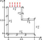
(a) Test setting with boundary conditions for $\boldsymbol{u}$.

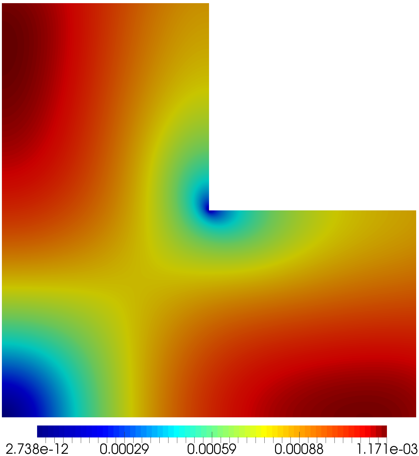
(b) Modulus $|\boldsymbol{u}|$ of $\boldsymbol{u}$ at time t = 3.0.

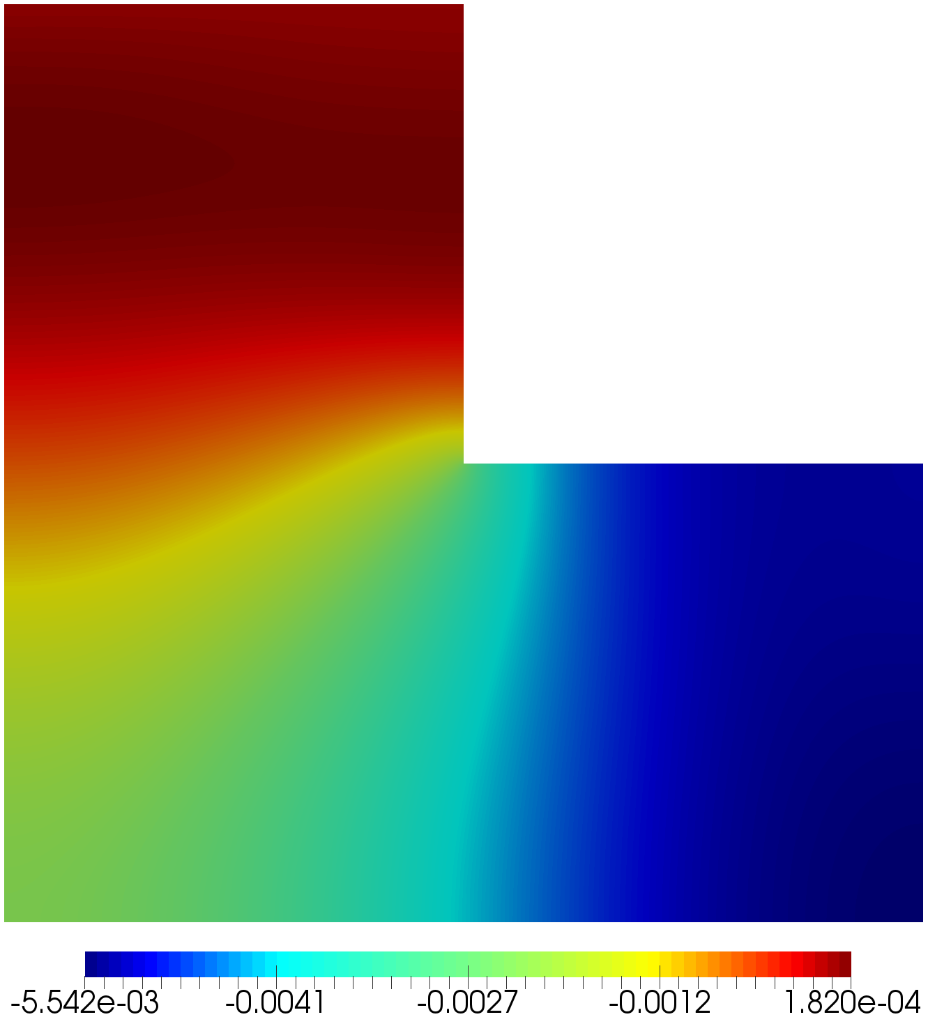
(c) Pressure $p$ at time t = 3.0.

Figure 4.1: Problem setting with boundary conditions for $\boldsymbol{u}$ and profile of the solution at time t = 3.8.

Fig. 4.2 and 4.3 illustrate and compare the results of our computations for the schemes presented in Problem 2.1 and 2.2, respectively. In Fig. 4.2, the convergence in space and time of the goal quantity $G_{\boldsymbol{u}}$ of (4.1) is clearly observed for either families of discretizations. In Fig. 4.3, the superiority of the higher order members of the dG($k$) and cG($k$) schemes is illustrated. The scheme dG(1) and, on the coarser time mesh, the scheme cG(2) are strongly erroneous. For the poroelasticity system (1.1), this illustrates the sensitivity of numerical predictions with respect to the time discretization and argues for higher order approaches that, however, put an additional facet of complexity on the efficient (iterative) solution of the algebraic equations; cf. [2]. Finally, in Tab. 4.1 characteristics of the computed goal quantities are summarized.

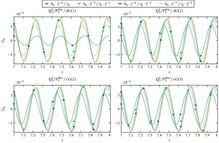
Figure 4.2: Computed goal quantity $G_{\boldsymbol{u}}$ of (4.1): Space-time convergence and accuracy of the schemes defined in Problem 2.1 and 2.2.

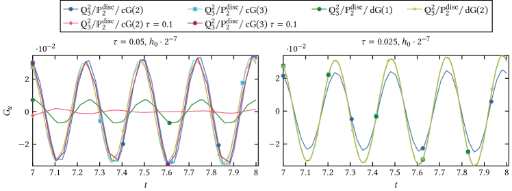
Figure 4.3: Computed goal quantity $G_{\boldsymbol{u}}$ of (4.1): Comparison of dG(1) and dG(2) of Problem 2.1 with cG(2) and cG(3) of Problem 2.2.

	$\min\{G_{p}(t)\mid t\in[7,8]\}$		$\max\{G_{p}(t)\mid t\in[7,8]\}$		$\min\{G_{\boldsymbol{u}}(t)\mid t\in[7,8]\}$		$\max\{G_{\boldsymbol{u}}(t)\mid t\in[7,8]\}$
$h\hphantom{{}_{7}}\;\;\tau\hphantom{{}_{3}}$	$cG(3)$	$dG(2)$	$cG(3)$	$dG(2)$	$cG(3)$	$dG(2)$	$cG(3)$	$dG(2)$
$h_{4}\;\;\tau_{0}$	-2.030e-02	-1.903e-02	2.046e-02	1.938e-02	-2.387e-02	-2.204e-02	2.386e-02	2.290e-02
$h_{5}\;\;\tau_{1}$	-2.581e-02	-2.534e-02	2.606e-02	2.570e-02	-2.947e-02	-2.937e-02	2.981e-02	2.964e-02
$h_{6}\;\;\tau_{2}$	-2.850e-02	-2.848e-02	2.876e-02	2.882e-02	-3.222e-02	-3.222e-02	3.266e-02	3.264e-02
$h_{7}\;\;\tau_{3}$	-2.984e-02	-2.985e-02	3.024e-02	3.025e-02	-3.345e-02	-3.350e-02	3.393e-02	3.399e-02

Table 4.1: Convergence and comparison of characteristics of the goal quantities $G_{p}$ and $G_{\boldsymbol{u}}$ in (4.1) for dG(2) and cG(3) with $\mathbb{Q}_{3}^{2}/\mathbb{P}_{2}^{\text{disc}}$ space discretization and $h_{j}=h_{0}\cdot 2^{-j}$ and $\tau_{j}=\tau_{0}\cdot 2^{-j}$.

References

• [1] M. Anselmann, M. Bause, A geometric multigrid method for space-time finite element discretizations of the Navier–Stokes equations and its application to 3d flow simulation, ACM Trans. Math. Softw., 49 (2023), Article No.: 5, pp. 1–25, https://doi.org/10.1145/3582492.
• [2] M. Anselmann, M. Bause, N. Margenberg, P. Shamko, An energy-efficient GMRES–Multigrid solver for space-time finite element computation of dynamic poro- and thermoelasticity, Comput. Mech., submitted (2023), pp. 1–30; arXiv:2303.06742.
• [3] M. Anselmann, M. Bause, Efficiency of local Vanka smoother geometric multigrid preconditioning for space-time finite element methods to the Navier–Stokes equations, PAMM Proc. Appl. Math. Mech., 22 (2022), doi:10.1002/pamm.202200088, pp. 1–6.
• [4] D. Arndt, W. Bangerth, B. Blais, M. Fehling, R. Gassmöller, T. Heister, L. Heltai, U. Köcher, M. Kronbichler, M. Maier, P. Munch, J.-P. Pelteret, S. Proell, K. Simon, B. Turcksin, D. Wells, J. Zhang, The deal.II Library, Version 9.3, J. Numer. Math., 29 (2021), pp. 171–186.
• [5] M. Bause, A. Anselmann, U. Köcher, F. A. Radu, Convergence of a continuous Galerkin method for hyperbolic-parabolic systems, Comput. Math. with Appl., submitted (2022), pp. 1–24; arXiv:2201.12014.
• [6] R. Becker, Mesh adaptation for Dirirchlet flow control via Nitsche’s method, Commun. Numer. Meth. Engrg., 18 (2002), pp. 669–680.
• [7] M. Biot, General theory of three-dimensional consolidation, J. Appl. Phys., 12 (1941), pp. 155–164.
• [8] M. Biot, Theory of elasticity and consolidation for a porous anisotropic solid, J. Appl. Phys., 26 (1955), pp. 182–185.
• [9] M. Biot, Theory of finite deformations of porous solids, Indiana Univ. Math. J., 21 (1972), pp. 597–620.
• [10] J. W. Both, N. A. Barnafi, F. A. Radu, P. Zunino, A. Quarteroni, Iterative splitting schemes for a soft material poromechanics model, Comput. Methods Appl. Mech. Engrg., 388 (2022), 114183.
• [11] M. Corti, P. F. Antonetti, L. Dede, A. M. Quarteroni, Numerical modelling of the brain poromechanics by high-order discontinuous Galerkin methods, arXiv:2210.02272, pp. 1–28.
• [12] D. E. Carlson, Linear thermoelasticity, Handbuch der Physik V Ia/2, Springer, Berlin, 1972.
• [13] S. Hussain, F. Schieweck, S. Turek, An efficient and stable finite element solver of higher order in space and time for nonstationary incompressible flow, Internat. J. Numer. Methods Fluids, 73 (2013), pp. 927–952.
• [14] S. Hussain, F. Schieweck, S. Turek, Higher order Galerkin time discretizations and fast multigrid solvers for the heat equation, J. Numer. Math., 19 (2011), pp. 41–61.
• [15] S. Jiang, R. Racke, Evolution equations in thermoelasticity, CRC Press, Boca Raton, 2018.
• [16] V. John, Finite Element Methods for Incompressible Flow Problems, Springer, Cham, 2016.
• [17] O. Karakashian, C. Makridakis, Convergence of a continuous Galerkin method with mesh modification for nonlinear wave equations, Math. Comp., 74 (2004), pp. 85–102.
• [18] U. Köcher, M. Bause, Variational space-time methods for the wave equation, J. Sci. Comput., 61 (2014), pp. 424–453.
• [19] R. Leis, Initial boundary value problems in mathematical physics, Teubner, Stuttgart, John Wiley & Sons, Chichester, 1986.
• [20] D. A. Di Pietro, A. Ern, Mathematical Aspects of Discontinuous Galerkin Methods, Springer, Berlin, 2012.
• [21] C. Seifert, S. Trostorff, M. Waurick, Evolutionary Equations: Picard’s Theorem for Partial Differential Equations, and Applications, Birkhäuser, Cham, 2022.
• [22] M. Slodička, Application of Rothe’s method to integrodifferential equation, Comment. Math. Univ. Carolinae, 30 (1989), pp. 57–70.