Contextualizing MLP-Mixers Spatiotemporally for Urban Data Forecast at Scale

Abstract.

Spatiotemporal urban data (STUD) displays complex correlational patterns. Extensive advanced techniques have been designed to capture these patterns for effective forecasting. However, because STUD is often massive in scale, practitioners need to strike a balance between effectiveness and efficiency by choosing computationally efficient models. An alternative paradigm called MLP-Mixer has the potential for both simplicity and effectiveness. Taking inspiration from its success in other domains, we propose an adapted version, named NexuSQN, for STUD forecast at scale. We identify the challenges faced when directly applying MLP-Mixers as series- and window-wise multivaluedness and propose the ST-contextualization to distinguish between spatial and temporal patterns. Experimental results surprisingly demonstrate that MLP-Mixers with ST-contextualization can rival SOTA performance when tested on several urban benchmarks. Furthermore, it was deployed in a collaborative urban congestion project with Baidu, specifically evaluating its ability to forecast traffic states in megacities like Beijing and Shanghai. Our findings contribute to the exploration of simple yet effective models for real-world STUD forecasting. The code is available at: https://github.com/tongnie/NexuSQN.

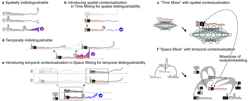
Figure 1. ST-contextualization in urban data: (a) If future series across locations differ but share a similar historical series, mixing time without knowing the location causes a series-wise multivaluedness. (b-c) The spatial context that distinguishes the locations is needed. (d) Even with spatial context enabled, if two windows with identical histories differ in the future, mixing space is window-wise indistinguishable. (e-f) The temporal context is necessary to disambiguate the multivaluedness.

1. Introduction

With the continued growth of infrastructure and environmental systems, a vast amount of urban data is being measured and collected. This data includes information on traffic flow, meteorological records, and energy consumption. Analyzing urban data can be challenging due to its partially observable dynamics, which include human interactions, information exchanges, and external perturbations. However, urban data also exhibits macroscopic spatiotemporal correlational patterns such as continuity, periodicity, and proximity (Nie et al., 2023a). These patterns have attracted the attention of many data-driven models that aim to capture them. Representative models are advanced spatial-temporal graph neural networks (STGNNs) and Transformers, which are increasingly popular and extensively studied due to their innovative designs to capture latent correlations in spatiotemporal data (Yu et al., 2018; Li et al., 2018; Wu et al., 2019; Bai et al., 2020; Wu et al., 2021; Zhou et al., 2022).

Meanwhile, urban data is massive in scale. For example, fine-grained traffic flow databases can contain more than 4 million data points (Liu et al., 2023c). Advanced techniques, such as recurrent graph topology and self-attention, have high computational complexity, making them computationally intensive for city-scale applications (Liu et al., 2023c; Jin et al., 2023; Cini et al., 2023a). Practitioners often need to strike a balance between effectiveness and efficiency by choosing simpler models and reducing complexity (Elsayed et al., 2021), particularly when resources are limited. Trading off effectiveness for efficiency becomes a pressing question.

To break the trade-off, recent studies have brought attention back to an alternative class of simple yet effective architectures called MLP-Mixers in various domains, such as vision (Tolstikhin et al., 2021), language (Fusco et al., 2022), and graph (He et al., 2023). This renewed interest in MLP-Mixers suggests that they may hold promise for both effectiveness and efficiency. This salient feature motivates us to investigate the potential of extending the MLP-Mixer paradigm to large-scale spatiotemporal urban data. We aim to achieve performance comparable to elaborate architectures while maintaining simplicity and scalability.

In the context of spatiotemporal data, limited pioneering work (Chen et al., 2023; Zhang et al., 2023; Zhong et al., 2023; Shao et al., 2022a; Yi et al., 2023) has explored the performance of MLP-Mixer on several forecasting benchmarks. However, we have found that applying it directly to a variety of real-world urban data will not yield desirable results. After thorough investigation and surveying related work, we have identified the problem that hinders its effectiveness: the issue of spatiotemporal contextualization. As illustrated in Fig. 1, spatiotemporal contextualization refers to a data pattern where multiple possible future series share similar historical series, causing a series- and windows-wise multivaluedness due to the parameter sharing across locations and times. This issue is frequently posed in urban spatiotemporal systems. For instance, macroscopic traffic flows can be indistinguishable as they miss the microscopic details such as individual trajectories. When working with this multivaluedness, univalued models such as MLP-Mixers may struggle to learn nondeterministic functions. This can result in mediocre performance and systemic errors that can be hard to further reduce. As a remedy, we reconstruct the contextualization information from spatiotemporal data itself to disambiguate multivaluedness and convert them into mappings as univalued as possible.

By extending the MLP-Mixers, in this paper, we present a scalable contextualized MLP-Mixer and investigate its application in large-scale urban data forecasting problems. To address the contextualization issue, we design a learnable embedding to form a binder for spatial-temporal interactions in the mixing layers. On top of this embedding, we parameterize the time-mixer with local adaptations and customize the space-mixer with interaction-aware mixing. The spatiotemporal context makes them distinguishable across location and time. To further adapt for the high-dimensionality of large urban databases, we preserve the scalability property using the kernel method, achieving an efficient architecture with linear complexity.

Through MLP-Mixers, our focus is to explore the practical performance of a minimalist model that only includes essential connections to directly express contextualization. To evaluate the effectiveness of our model, we conduct forecasting tasks on 14 public urban benchmarks, which cover data on traffic, energy, and the environment. Our extensive experiments, which include short-term, long-term, and large-scale forecasting tasks, reveal a surprising result – after being spatiotemporally contextualized, MLP-Mixer can perform comparably or even surpass its more complex counterparts. Remarkably, even a single space-mixing layer can achieve competitive performance on most benchmarks. Furthermore, MLP-Mixer offers advantages such as faster computation, lower resource consumption, a smaller model size and flexibility to transfer.

We also demonstrate its effectiveness in real-world deployment. We conducted an urban congestion project in collaboration with Baidu. First, we examined its scalability to predict the propagation of large-scale congestion at the regional level in three megacities in China that contain tens of thousands of road sections. Second, we conducted online parallel tests in the generation of fine-grained congestion maps in production environments using Baidu Map’s API. To summarize, our main technological contributions include:

1. We identify the main bottlenecks of MLP-Mixers as spatiotemporal contextualization in urban data forecasting;

2. We present a simple-yet-effective remedy to address the contextualization issue and propose a scalable architecture;

3. We showcase its superiority in accuracy, efficiency, and flexibility by comparing it to SOTA in 14 urban benchmarks;

4. We deploy it in real-world large-scale urban traffic applications and demonstrate its practical effectiveness.

We hope this work will incentivize further endeavors to adopt and extend MLP-Mixers to more challenging urban computing problems. As we aim to identify the essential components, we name our model Nexus Sine Qua Non (NexuSQN) networks – a name that literally means “the connection without which it could not be.”

2. Preliminary and Related Work

Notations and Problem Statement

We first introduce some notations following the terminology in (Cini et al., 2022). In an urban sensor network with $N$ static sensors on some locations, four types of data are considered: (1) $\mathcal{X}_{t-T+1:t}\in\mathbb{R}^{N\times T\times d_{\text{in}}}$: The data tensor collected by all sensors over a time interval $\mathcal{T}=\{t-T+1,\dots,t\}$, where $T$ represents the time window size, and $d_{\text{in}}$ is the length of the measurement at each sensor at each timestamp; (2) $\mathbf{A}_{t}\in\mathbb{R}^{N\times N}$: An adjacency matrix can be either predefined or adaptive; (3) ${\mathbf{U}_{t-T+1:t}\in\mathbb{R}^{T\times d_{\text{u}}}}$: Exogenous variables, such as time of day and day of the week information; (4) ${\mathbf{V}\in\mathbb{R}^{N\times d_{\text{v}}}}$: Node-specific features, such as sensor IDs. We denote the variables and features at each time step by the subscript $t$. It should be noted that this paper uses the terms node, sensor, and location interchangeably. A graph signal with a window size of $T$ is defined by the following 4-tuple: $\mathcal{G}_{t-T+1:t}=\left(\mathcal{X}_{t-T+1:t},\{\mathbf{U}_{t},\mathbf{A}_{t}|t\in\mathcal{T}\},\mathbf{V}\right)$. Spatiotemporal data forecasting (STDF) is therefore defined as learning a function ${F(\cdot|\theta)}$ parameterized by $\theta$ that maps to the next $H$ time steps of graph signals $\widehat{\mathcal{G}}_{t+1:t+H}$ from a given historical graph signal $\mathcal{G}_{t-T+1:t}$.

MLP-Mixer

Recent years have witnessed a comeback of MLP-based methods (e.g., MLP-Mixer) due to its simplicity and effectiveness (Tolstikhin et al., 2021; He et al., 2023). The canonical MLP-Mixer model for STDF (Chen et al., 2023) can be formulated in a compact form as follows:

(1) $$\mathbf{Y}=\textsc{MLP}_{\text{time}}(\textsc{MLP}_{\text{channel}}(\mathcal{X}_{t-T+1:t},\text{dim}=0),\text{dim}=1),$$

where $\textsc{MLP}_{\text{time}}$ and $\textsc{MLP}_{\text{channel}}$ alternatively perform mixing operation along temporal and spatial dimensions, respectively. Although recent work has already shown that the MLP-based architecture can be a competitive baseline for STDF (Zeng et al., 2022; Shao et al., 2022a; Chen et al., 2023; Zhang et al., 2023; Yi et al., 2023; Zhong et al., 2023), however, pure MLP model has been proven to be a good overfitter (He et al., 2023) and easily falls into undesirable local suboptimal solutions.

Related Work

As the leading approaches for STDF, STGNNs and Transformers use advanced techniques such as GNNs, RNNs and self-attention to exploit spatiotemporal correlations for effective forecasting. Extensive studies have shown promising results using them (Yu et al., 2018; Li et al., 2018; Wu et al., 2019; Bai et al., 2020; Guo et al., 2019; Zheng et al., 2020; Wu et al., 2021; Zhou et al., 2022; Nie et al., 2022). Although existing architectures perform well, they can require a high complexity to implement. Previous research has attempted to address this scalability issue by simplifying the architecture or using better embedding techniques.

Among the limited studies on simplified and scalable methods for STDF, Cini et al. (2022) proposed scalable STGNNs based on preprocessing that encode data features prior to training. Liu et al. (2023b) replaced the GNNs with alternative spatial techniques and used a graph sampling strategy to improve performance. Both of the methods elaborate temporal encoders and pre-computed graph features. TS-Mixer (Chen et al., 2023), MLPST (Zhang et al., 2023), FreTS (Yi et al., 2023), ST-MLP (Wang et al., 2023), PITS (Lee et al., 2023) and MSD-Mixer (Zhong et al., 2023) studied the effectiveness of MLP-based architectures in medium-sized forecasting benchmarks and showed promising performance. In another vein of research, several methods have emerged to challenge Transformer-based models existing for long-term series forecasting (LTSF), such as LightTS (Zhang et al., 2022), DLinear (Zeng et al., 2022), and TiDE (Das et al., 2023). Most of them adopt a channel independence assumption and do not include explicit relational modeling.

Regarding embedding methods for spatiotemporal data, Shao et al. (2022a) used learnable embeddings for all nodes, time of day, and day of week points. This approach enables MLPs to achieve competitive performance on several datasets. However, using overparameterized embedding can lead to redundancy and overfitting. Cini et al. (2023b) offered further interpretation of node embedding as local effects and integrated it into a global-local architecture.

In summary, STGNNs and Transformers have been extensively studied in STDF, but MLP-Mixers for large-scale urban data have been less investigated, leaving opportunities for us to contribute.

3. ST-Contextualized MLP-Mixers

To address the contextualization issue, this section demonstrates the proposed NexuSQN model. NexuSQN is a simple yet effective architecture that features a full MLP-based structure with spatial-temporal interactions, as shown in Fig. 1. Notably, it leverages the structured mixing operations to contextualize the STDF task, allowing it to bypass the need for complex temporal methods (e.g., RNN, TCN, and self-attention) and spatial techniques (e.g., diffusion convolution and predefined graph). It also achieves a linear complexity with respect to the length of the sequence and the number of series.

3.1. Overview of Architectural Components

Overview

The overall architecture of NexuSQN can be concisely formulated as follows:

(2) $$\mathbf{H}^{(1)}=\textsc{TimeMixer}(\mathcal{X}_{t-T+1:t};\mathbf{E}_{t-T+1:t}),$$

$$\mathbf{H}^{(l+1)}=\textsc{SpaceMixer}(\mathbf{H}^{(l)};\mathbf{E}_{t-T+1:t}),~{}l\in\{1,\dots,L\},$$

$$\mathcal{X}_{t+1:t+H}=\textsc{Readout}(\mathbf{H}^{(L+1)}),$$

where the TimeMixer and SpaceMixer modules are extending the conceptually simple MLP-Mixers to consider spatiotemporal contextualization. Importantly, $\mathbf{E}_{t-T+1:t}$ represents the spatiotemporal node embedding. Readout module contains a Mlp and a reshaping layer to directly output multistep predictions. As shown, only one time-mixing operation is performed, followed by $L$ space-mixing layers. Interestingly, we find that a single SpaceMixer can achieve competitive performance on most benchmarks.

Spatiotemporal Node Embedding

To address the contextualization issue, we use the versatility of node embedding as a structural cornerstone and enable it to form a binder for spatial-temporal interactions in the mixing layers. It mimics the positional and structural representations in the theory of GNNs’ expressivity (Srinivasan and Ribeiro, 2019).

Learnable node embedding has been adopted as a positional encoding in both spatiotemporal and general graphs (Shao et al., 2022a; Dwivedi et al., 2022; Cini et al., 2023b). Given $N$ nodes, it can be instantiated as a randomly initialized dictionary $\mathbf{E}\in\mathbb{R}^{N\times d_{\text{emb}}}$. However, it only reflects the static features of each series, such as the dominating patterns, and is agnostic to temporal variation. To address this, we propose incorporating the stationary property of time series, such as periodicity and seasonality. We use sinusoidal positional encoding (Vaswani et al., 2017) $\mathbf{U}_{t-T+1:t}\in\mathbb{R}^{T\times d_{\text{u}}}$ to inform the static embedding with the time-of-day context. Specifically, we first project the node embedding and the time stamp encoding to a matched dimension and fuse them with a MLP:

(3) $$\widetilde{\mathbf{U}}=\mathbf{W}_{\text{u}}\mathbf{U}_{t-T+1:t},~{}\widetilde{\mathbf{E}}=\mathbf{E}\mathbf{W}_{\text{e}},$$

$$\mathbf{E}_{t-T+1:t}=\textsc{Mlp}(\widetilde{\mathbf{E}}\widetilde{\mathbf{U}}^{\mathsf{T}}),$$

where $\mathbf{W}_{\text{u}}\in\mathbb{R}^{D\times T}$ and $\mathbf{W}_{\text{e}}\in\mathbb{R}^{d_{\text{emb}}\times d_{\text{u}}}$ are linear transforms, and $\mathbf{E}_{t-T+1:t}\in\mathbb{R}^{N\times D}$ is the final spatiotemporal node embedding (STNE). When inputs from different time intervals exhibit varying sinusoidal patterns, STNE is capable of capturing the periodicity of a time series, which constructs a dynamic representation.

3.2. Flattened Dense Time-Mixers

Dimension Flattening and Projection

STGNNs usually handle time and feature dimensions separately. This involves first independently projecting the input features at each time step to high-dimensional features and then correlating different time steps with sequential models such as RNNs. While this treatment is reasonable and intuitive, it significantly increases model complexity and the risk of overfitting, especially when the hidden size is much larger than the feature dimension. To address this issue, we propose to flatten the input series along the time dimension and project it into the high-dimensional hidden space using a single MLP:

(4) $$\mathbf{X}_{t-T+1:t}=\texttt{FOLD}(\mathcal{X}_{t-T+1:t}),$$

$$\mathbf{H}^{(0)}=\textsc{Mlp}(\mathbf{X}_{t-T+1:t}),$$

where $\texttt{FOLD}(\cdot):\mathbb{R}^{N\times T\times d_{\text{in}}}\rightarrow\mathbb{R}^{N\times Td_{\text{in}}}$ represents the flattening operator. By flattening and projecting along the time axis, serial information is stored in the hidden state $\mathbf{H}^{(0)}\in\mathbb{R}^{N\times D}$.

Time Mixing with Spatial Context

To further encode the temporal relations and patterns underlying the historical series, TimeMixer further adopts a two-layer feedforward Mlp for time mixing:

(5) $$\widetilde{\mathbf{H}}^{(0)} =\textsc{Mlp}(\mathbf{H}^{(0)}),$$

$$\mathbf{H}^{(1)} =\texttt{LayerNorm}(\widetilde{\mathbf{H}}^{0}+\textsc{MLP}(\mathbf{H}^{(0)})),$$

where $\mathbf{H}^{(1)}$ is the time-mixed representation, and $\texttt{LayerNorm}(\cdot)$ is adopted to reduce the variance between multivariate series (Liu et al., 2023a).

It is observed that Eqs. (5) and (4) are global models shared by all series. When given two sensors with similar historical input but different dynamics in the future, these global models can fail to contextualize each series in spatial dimension, causing a series-wise multivaluedness. A straightforward way to adapt the global model to each series is to set a specialized encoder for each one, that is:

(6) $$\widetilde{\mathbf{h}}_{i}^{(0)}=\textsc{Mlp}_{i}(\mathbf{h}_{i}^{(0)}),\forall i=\{1,\dots,N\}.$$

However, such an overparameterization is undesirable and prone to overfitting. To address this issue, we customize each node with a discriminative identifier using STNE directly. Specifically, we concatenate $\mathbf{E}_{t-T+1:t}$ to all series in the first Mlp of TimeMixer in Eq. (5) as spatial context for distinguishable time mixing:

(7) $$\widetilde{\mathbf{h}}_{i}^{(0)}=\textsc{Mlp}([\mathbf{h}_{i}^{(0)}\|\mathbf{e}_{i}^{t}]),\forall i=\{1,\dots,N\},$$

which yields:

(8) $$[\mathbf{h}_{i}^{(0)}\|\mathbf{e}_{i}^{t}]\mathbf{\Theta}=[\mathbf{h}_{i}^{(0)}\|\mathbf{e}_{i}^{t}]\left[\begin{aligned} \mathbf{\Theta}_{1}\\ \mathbf{\Theta}_{2}\end{aligned}\right]=\mathbf{h}_{i}^{(0)}\mathbf{\Theta}_{1}+\mathbf{e}_{i}^{t}\mathbf{\Theta}_{2},$$

where $\mathbf{\Theta}_{1}$ is the global component shared by all nodes, while $\mathbf{e}_{i}\mathbf{\Theta}_{2}$ is the specialized local adaptation of each individual.

The introduction of learnable embeddings for each node is equivalent to the specialization of the global model, which improves the use of local dynamics specific to nodes (Cini et al., 2023b). We also find that adding STNE to each series can be treated as incorporating low-frequency components into high-frequency representations. This highlights the impact of local events on urban spatiotemporal data.

3.3. Structured Scalable Space-Mixers

To model the multivariate correlations of series, the canonical MLP-Mixers for space mixing is:

(9) $$\bar{\mathbf{h}}^{d}=\sigma(\mathbf{\Theta}_{\text{channel}}\mathbf{h}^{d}+\mathbf{b}),$$

or: $$\bar{h}_{n}=\sigma(\sum_{j=1}^{N}\theta_{n,j}h_{j}+b_{n}),~{}n\in\{1,\dots,N^{\prime}\},$$

where $\bar{\mathbf{h}}^{d}\in\mathbb{R}^{N^{\prime}}$ is the graph state at dimension $d$, and $\mathbf{\Theta}_{\text{channel}}\in\mathbb{R}^{N^{\prime}\times N}$ is channel mixing parameter. The unconstrained mixing weight $\theta_{n,j}$ is shared by all time windows and is agnostic to the absolute position in the sequence, rendering it incapable of contextualizing the series in temporal dimension, causing a window-wise multivaluedness. For instance, a sensor’s readings may differ at two different windows but share a similar historical series. In addition, the mixed message from $h_{j}$ depends only on the state of node $j$ and is agnostic to the temporal pattern of $h_{n}$. The interaction between two temporal patterns should also be considered.

A remedy for this issue is to assign a unique identifier to each time point. However, this approach has two issues: (1) time-independent model relies on relative timestamps and using absolute ones is difficult for it; (2) timestamp-based encoding can attribute the ambiguity to static factors, such as time of day feature, but this could be caused by time-varying dynamics and specific temporal patterns.

Space Mixing with Temporal Context

To enable the SpaceMixer to become time-varying and adaptive to the interactive temporal context within time windows, we consider a pattern-aware mixing:

(10) $$\bar{h}_{n}=\sigma(\sum_{j=1}^{N}\mathcal{F}_{t}(\mathbf{h}^{d})h_{j}+b_{n}),~{}n\in\{1,\dots,N^{\prime}\},$$

where $\mathcal{F}_{t}(\cdot)$ represents a data-dependent function, such as self-attention. To implement, we set the mixed dimension $N^{\prime}=N$ to preserve the spatial dimension and formulate a structured SpaceMixer:

(11) $$\mathbf{m}_{i\leftrightarrow j}^{(l+1)}=\textsc{Contx}_{l}(\mathbf{h}_{i}^{(l)},\mathbf{h}_{j}^{(l)})=\Psi(\mathbf{h}_{i}^{(l)}\|\mathbf{h}_{j}^{(l)})[\mathbf{h}_{i}^{(l)}\|\mathbf{h}_{j}^{(l)}],$$

$$\mathbf{m}_{i}^{(l+1)}=\textsc{Mix}(\mathbf{m}_{i\leftrightarrow j}^{(l+1)};\forall j=\{1,\dots,N\})=\sum_{j=1}^{N}\mathbf{m}_{i\leftrightarrow j}^{(l+1)},$$

$$\mathbf{h}_{i}^{(l+1)}=\textsc{Update}_{l}(\mathbf{h}_{i}^{(l)},\mathbf{m}_{i}^{(l+1)})=\sigma(\mathbf{\Theta}\mathbf{h}_{i}^{(l)}+\mathbf{m}_{i}^{(l+1)}),$$

where $\mathbf{h}_{i}^{(l)}$ is the representation of node $i$ in layer $l$, and $\mathbf{\Theta}$ is the feedforward weight. $\Psi$ is the temporal contextualization function.

Compared to MLP-Mixer $\mathbf{H}^{(l)}=\sigma(\mathbf{\Theta}^{(l)}_{\text{channel}}\mathbf{H}^{(l-1)}\mathbf{\Theta}^{(l)}_{\text{time}})$, Eq. (11) customizes the channel mixing weight $\mathbf{\Theta}_{\text{channel}}$ with structured function $\Psi(\mathbf{h}_{i}^{(l-1)}\|\mathbf{h}_{j}^{(l-1)})$. Note that the contextualization function should be specified to be aware of the specific temporal interactions and positions at current window, $\Psi$ requires the pairwise correlating of node features. However, such a global operation costs $\mathcal{O}(N^{2})$ complexity, making it inefficient for large-scale networks. To address this scalability issue, we propose a scalable kernelized mixing using the STNE directly to reparameterize Eq. (11).

Scalable Kernelized Contextualization

Recall that $\mathbf{E}_{t-T+1:t}$ not only includes time information but can also be used as an agent to measure interactions between different series. To this end, we suggest reusing the STNE as a query for all available references to contextualize temporal patterns. Specifically, the temporal query $\langle\mathbf{e}_{i}^{t},\mathbf{e}_{j}^{t}\rangle$ can be treated as the vector inner product in the Hilbert space $\mathcal{H}$. Define a kernel function $\mathcal{K}:\mathcal{X}\times\mathcal{X}\rightarrow\mathbb{R}$, it admits:

(12) $$\mathcal{K}(\mathbf{e}_{i}^{t},\mathbf{e}_{j}^{t})=\langle\phi(\mathbf{e}_{i}^{t}),\phi(\mathbf{e}_{j}^{t})\rangle_{\mathcal{H}},$$

where $\phi:\mathcal{X}\rightarrow\mathbb{H}$ is a mapping function. Typically, the kernel method directly defines the kernel function and bypasses the explicit form of $\phi$. Instead, if we approximate the contextualization function $\Psi(\mathbf{h}_{i}^{(l-1)}\|\mathbf{h}_{j}^{(l-1)})$ using the kernel definition, we have:

(13) $$({\Psi}\mathbf{H})_{i} =\frac{\sum_{j=1}^{N}\mathcal{K}(\mathbf{e}_{i}^{t},\mathbf{e}_{j}^{t})\mathbf{h}_{j}}{\sum_{j=1}^{N}\mathcal{K}(\mathbf{e}_{i}^{t},\mathbf{e}_{j}^{t})}=\frac{\sum_{j=1}^{N}(\phi(\mathbf{e}_{i}^{t,\mathsf{T}})\cdot\phi(\mathbf{e}_{j}^{t}))\mathbf{h}_{j}^{\mathsf{T}}}{\sum_{j=1}^{N}\phi(\mathbf{e}_{i}^{t,\mathsf{T}})\cdot\phi(\mathbf{e}_{j}^{t})},$$

where the conditional probability $p(\mathbf{e}_{j}^{t}|\mathbf{e}_{i}^{t})=\frac{\mathcal{K}(\mathbf{e}_{i}^{t},\mathbf{e}_{j}^{t})}{\sum_{j=1}^{N}\mathcal{K}(\mathbf{e}_{i}^{t},\mathbf{e}_{j}^{t})}$ is a linearized kernel smoother (Tsai et al., 2019). The above process can be simplified using the associative property of matrix multiplication:

(14) $$({\Psi}\mathbf{H})_{i}=\frac{\phi(\mathbf{e}_{i}^{t,\mathsf{T}})\sum_{j=1}^{N}(\phi(\mathbf{e}_{j}^{t})\mathbf{h}_{j}^{\mathsf{T}})}{\phi(\mathbf{e}_{i}^{t,\mathsf{T}})\sum_{j=1}^{N}\phi(\mathbf{e}_{j}^{t})}.$$

In this way, we can compute the above equation in $\mathcal{O}(N)$ time and space complexity with a proper kernel function. Using Eq.(14), SpaceMixer can efficiently capture pairwise interactions among windows as the temporal context for distinguishable space mixing.

Since $\mathbf{E}_{t}$ contains the time-of-day feature, this query function can vary over time. This makes our approach lie between time-dependent and data-dependent routines, allowing it to forecast using both relative timestamps and interactive temporal patterns. Furthermore, it models the positional embeddings and structural representations simultaneously in spatiotemporal graphs (Srinivasan and Ribeiro, 2019).

Table 1. Statistics of public urban computing benchmarks.

Datasets		Type	Steps	Nodes	Edges	Interval
Traffic	METR-LA	speed	34,272	207	1,515	5 min
	PEMS-BAY	speed	52,128	325	2,369	5 min
	PEMS03	volume	26,208	358	546	5 min
	PEMS04	volume	16,992	307	340	5 min
	PEMS07	volume	28,224	883	866	5 min
	PEMS08	volume	17,856	170	277	5 min
	TrafficL	occupancy	17,544	862	-	60 min
	LargeST-GLA	volume	525,888	3,834	98,703	15 min
Energy	Electricity	electricity	26,304	321	-	60 min
	CER-EN	smart meters	52,560	6,435	639,369	10 min
	PV-US	solar power	52,560	5,016	417,199	10 min
Environ.	AQI	pollutant	8,760	437	2,699	60 min
	Global Temp	temperature	17,544	3,850	-	60 min
	Global Wind	wind speed	17,544	3,850	-	60 min

Table 2. Results on METR-LA, PEMS-BAY, PEMS03, PEMS04, PEMS07, and PEMS08 datasets (in: 12 steps, out: 12 steps).

Dataset	METR-LA	PEMS-BAY	PEMS03	PEMS04	PEMS07	PEMS08
Metric	MAE	MAE	MAE	MAE	MAE	MAE
AGCRN	3.14	1.63	15.58	18.90	20.64	15.23
DCRNN	3.20	1.67	15.90	20.75	22.30	16.06
GWNet	3.09	1.59	14.66	18.95	21.13	15.02
GatedGN	3.01	1.58	17.08	18.81	22.68	14.91
GRUGCN	3.46	1.77	16.62	22.68	24.37	17.55
EvolveGCN	3.81	1.95	19.11	26.21	28.40	20.64
ST-Transformer	3.52	1.77	15.85	21.63	23.05	16.00
STGCN	3.23	1.66	15.61	20.95	22.53	16.20
STID	3.13	1.58	15.27	18.60	19.88	14.32
MTGNN	3.07	1.58	14.70	18.48	20.19	14.57
D2STGNN	3.05	1.55	14.45	18.39	20.84	14.52
DGCRN	3.07	1.59	14.73	18.77	21.24	14.70
SCINet	3.47	1.82	15.43	19.19	23.11	15.77
NexuSQN	2.95	1.54	14.18	18.03	19.28	13.98

4. Evaluation on Public Benchmarks

Extensive experiments are carried out to compare NexuSQN with state-of-the-art neural forecasting baselines in 14 well-known urban computing benchmarks. To validate its effectiveness in real-world applications, we further conduct a collaborative urban congestion project with Baidu in 5 large-scale urban road networks. Experimental setups and results are summarized below. Details and supplementary results are given in the appendix. Model implementations are publicly available at: https://github.com/tongnie/NexuSQN.

4.1. Experiment Setup

Datasets

Numerous experiments were conducted to comprehensively evaluate models’ predictive capabilities. These benchmarks included short-term, long-term, large-scale, and non-graph forecasting, ranging from traffic flow, environmental measurements, and engergy records. Brief statistics information is provided in Tab. 1, and detailed descriptions can be found in the appendix.

Baselines

We consider a variety of baseline models from the literature, including STGNNs for shot-term forecasting: STGCN (Yu et al., 2018); DCRNN (Li et al., 2018); GWNet (Wu et al., 2019); AGCRN (Bai et al., 2020); EvolveGCN (Pareja et al., 2020); ST-Transformer (Xu et al., 2020); MTGNN (Wu et al., 2020); GatedGN (Satorras et al., 2022); GRUGCN (Gao and Ribeiro, 2022); STID (Shao et al., 2022a); D2STGNN (Shao et al., 2022b); DGCRN (Li et al., 2023). And long-term series forecasting models: Autoformer (Wu et al., 2021); Informer (Zhou et al., 2021); FEDformer (Zhou et al., 2022); Pyraformer (Liu et al., 2022a); StemGNN (Cao et al., 2020); SCINet (Liu et al., 2022b); DLinear (Zeng et al., 2022); PatchTST (Nie et al., 2022); TimesNet (Wu et al., 2022).

4.2. Results on Traffic Benchmarks

Short-term Performance

Results of model comparison on short-term traffic flow benchmarks are shown in Table 2. In general, our model achieves comparable or even superior performance compared to its more complicated counterparts. Compared to STID, NexuSQN features the exploitation of relational structures with distinguishable space mixing, thus showing better accuracy in all scenarios. Additionally, advanced STGNNs such as MTGNN, and D2STGNN also show competitive results. However, high computational complexity requires them to consume much more memory and training times. Although our model does not depend on predefined graphs, it still achieves promising performance in traffic data. This observation echoes our previous finding that although distance-based adjacency matrices may reflect traffic speed patterns, they are not sufficient to understand traffic volume patterns (Nie et al., 2023b). Finally, it is important to note that our model only contains one single SpaceMixer layer in all traffic benchmarks. This finding surprisingly demonstrates the effectiveness of a minimalist structure for traffic forecasting.

Table 3. Long-term results on TrafficL (in: 96, out: 384).

Dataset	TrafficL
Metric	96	192	288	384	Ave.
	MAE	MAE	MAE	MAE	NMAE	MRE
Autoformer	1.34	1.43	1.82	2.07	2.38	27.90
Informer	1.35	1.44	1.80	2.00	2.35	27.72
DLinear	1.30	1.41	1.74	1.92	2.14	25.73
TimesNet	1.31	1.41	1.43	1.52	1.88	22.60
SCINet	1.21	1.40	1.41	1.47	1.86	22.27
NexuSQN	1.11	1.18	1.19	1.28	1.63	19.55

Table 4. Large-scale results on LargeST (in: 12, out: 12).

Dataset	LargeST-GLA
Metric	3	6	12	Ave.
	MAE	MAE	MAE	MAE	Time (h)
AGCRN	18.64	22.01	26.91	21.99	38
DCRNN	18.64	23.58	31.41	23.68	69
GWNet	16.42	19.87	24.59	19.70	31
STGCN	19.16	24.69	33.33	24.76	15
MTGNN	17.30	20.24	24.56	20.18	26
NexuSQN	16.15	19.48	24.09	19.33	1.5

Long-term Performance

We also evaluate the model’s performance in long-term forecasting. Table 4 shows the results for different prediction horizons with a historical series of 96 steps. Compared to three strong baselines in the LTSF literature, NexuSQN shows great potential in this challenging task. This can be attributed to the encoding of both relative timestamps and local patterns.

Large-Scale Forecasting Performance

We adopt the LargeST benchmark (Liu et al., 2023c) to evaluate the performance on large-scale traffic networks. Tab. 4 shows that even with a single SpaceMixer layer, our model can outperform the complicate STGNNs. Furthermore, many advanced models such as D2STGNN and DGCRN are not applicable due to high memory consumption. Instead, NexuSQN can converge in less than 1.5 hours on such a billion-level dataset, which is an order of magnitude speed-up ($\geq$10x) compared to the STGNNs.

4.3. Results on Energy Benchmarks

Table 5. Long-term results on Electricity (in: 336, out: 96).

Dataset	Electricity
Models	NexuSQN	DLinear	TimesNet	SCINet
Metric	MAE	MAE	MAE	MAE
24	178.87	185.35	269.67	197.77
48	209.41	215.58	276.89	241.24
72	225.33	228.43	283.32	246.48
96	234.89	236.07	293.13	252.44
MAE	206.34	212.25	276.86	225.40
MRE	7.66	7.89	10.29	8.38
MAPE	12.97	15.05	15.53	18.67

Table 6. Large-scale results on CER-En (in: 36, out: 22).

Dataset	CER-En
Models	NexuSQN	GWNet	DCRNN	DLinear
Metric	MAE	MAE	MAE	MAE
0.5 h	0.21	0.23	0.22	0.23
7.5 h	0.26	0.34	0.28	0.30
11 h	0.27	0.35	0.28	0.31
MAE	0.25	0.31	0.27	0.29
MRE	0.42	0.51	0.45	0.49
MSE	0.37	0.59	0.46	0.49

Table 7. Large-scale results on PU-VS (in: 36, out: 22).

Dataset	PV-US
Models	NexuSQN	DCRNN	GWNet	GatedGN	GRUGCN	STGCN	MTGNN	DLinear	TimesNet
Metric	MAE	MAE	MAE	MAE	MAE	MAE	MAE	MAE	MAE
0.5 h	1.30	1.65	1.48	1.61	1.44	1.88	1.81	1.59	1.47
7.5 h	2.64	2.94	6.13	3.23	2.89	6.83	3.11	3.11	2.75
11 h	2.69	3.16	7.66	3.06	2.96	7.68	3.14	3.08	2.80
MAE	2.31	2.79	4.86	2.74	2.62	5.47	2.96	3.27	2.51

The results on long-term Electricity benchmark is shown in Tab. 6, and two large-scale datasets in Tabs. 6 and 7. Although advanced STGNNs achieve competitive performance in medium-sized traffic data, many of them run out of memory on the large-scale energy dataset. Similarly, NexuSQN consistently achieves superior performances under various settings. It is worth commenting that NexuSQN is the only method in the literature related to STGNNs and LTSF that performs well on all of these tasks.

4.4. Results on Environment Benchmarks

Environmental records such as weather and air quality contain complicated spatiotemporal processes that are challenging to forecast. We further evaluate models’ generality using air quality and meteorological data. Results in Tabs. 9 and 9 indicate the great potential of NexuSQN to handle time series with complex spatial structures and missing data. Even without popular sequential modeling techniques or advanced spatial models, it still achieves desirable results.

Table 8. Results on Weather (in: 48, out: 24). Results of baselines are from (Wu et al., 2023b).

Datasets	Wind		Temp
Metrics	MSE	MAE	MSE	MAE
N-BEATS	4.12	1.39	9.20	2.12
Longformer	4.47	1.49	17.35	3.14
Informer	4.93	1.58	33.29	4.42
Autoformer	4.69	1.47	10.14	2.25
Prayformer	4.61	1.51	23.33	3.67
FEDformer	4.75	1.50	11.05	2.41
ETSformer	5.09	1.59	9.76	2.27
N-HiTS	4.03	1.38	9.35	2.09
StemGNN	4.07	1.39	13.93	2.75
Corrformer	3.89	1.30	7.71	1.89
NexuSQN	3.52	1.29	7.43	1.87

Table 9. Results on AQI benchmark (in: 24, out: 3).

Dataset	AQI
Metric	1 h	2 h	3 h	Ave.
	MAE	MAE	MAE	MAE
AGCRN	10.78	14.32	16.96	14.02
DCRNN	9.89	13.79	16.78	13.49
GWNet	9.39	12.98	15.71	12.70
GatedGN	10.39	14.68	17.76	14.28
GRUGCN	10.02	13.95	16.92	13.63
EvolveGCN	10.64	15.02	18.27	14.64
STGCN	9.63	13.47	16.47	13.19
STID	10.44	14.76	17.88	14.36
MTGNN	10.24	14.10	16.83	13.72
D2STGNN	9.48	12.91	15.44	12.61
NexuSQN	9.43	12.90	15.45	12.58

4.5. Model Analysis

Table 10. Ablation studies on METR-LA and PEMS03 data.

Datasets		METR-LA				PEMS03
Variations		Full	w/o $\mathbf{E}_{T}$	w/ $\mathbf{A}_{\text{pre}}$	w/o SpaceMixer	Full	w/o $\mathbf{E}_{T}$	w/ $\mathbf{A}_{\text{pre}}$	w/o SpaceMixer
Metric		MAE	MAE	MAE	MAE	MAE	MAE	MAE	MAE
15 min		2.66	2.88	2.64	2.84	13.15	14.85	13.48	14.64
30 min		2.99	3.32	2.98	3.23	14.20	16.62	14.54	15.91
60 min		3.36	3.76	3.38	3.65	15.79	18.68	15.95	17.45
Ave.	MAE	2.95	3.25	2.95	3.18	14.18	16.46	14.45	15.76
	MSE	35.35	39.97	35.89	39.40	603.29	766.64	610.47	676.63

Ablation Study

Ablation studies are conducted to test the effectiveness of the model designs. Table 10 presents the forecasting performance of different model variations. “w/o $\mathbf{E}_{T}$” indicates that the ST-contextualization is removed and the model degrades into a MLP-Mixer. “w/ $\mathbf{A}_{\text{pre}}$” incorporates predefined graphs with additional diffusion graph convolutions (Li et al., 2018). “w/o SpaceMixer” means that we remove the SpaceMixer layer. The results clearly justify the effectiveness of the model designs of NexuSQN.

Selection of Kernels

We evaluate the impacts of different kernel methods in Tab. 11. As can be seen, the softmax kernel achieves the best performance, suggesting that the normalization and nonlinearity property of kernels can help to maintain the competitiveness of shallow NexuSQN with deep multi-layer STGNNs or Transformers.

Table 11. Performance of different kernels.

Datasets		PEMS08
Kernels $\phi(x)=$		$\texttt{softmax}(x)$	$\texttt{elu}(x)+1$	$\texttt{relu}(x/|x|)$	$\texttt{exp}(x)$	$x/|x|$
Metric		MAE	MAE	MAE	MAE	MAE
15 min		13.17	13.73	13.28	13.79	13.30
30 min		13.96	14.75	14.05	14.81	14.12
60 min		15.28	16.56	15.38	16.68	15.53
Ave.	MAE	13.98	14.79	14.08	14.87	14.15
	MAPE	9.02	9.55	9.14	9.68	9.23

Spatiotemporal Contextualization

We provide an example of the spatial contextualization effect in Fig. 2. The example in temporal dimension is provided in the appendix. As can be seen, the correlation of multivariate series can show distinct patterns between historical and future windows. With the design of spatiotemporally contextualized mixers, our model can distinguish different short-term patterns and forecast the true trend.

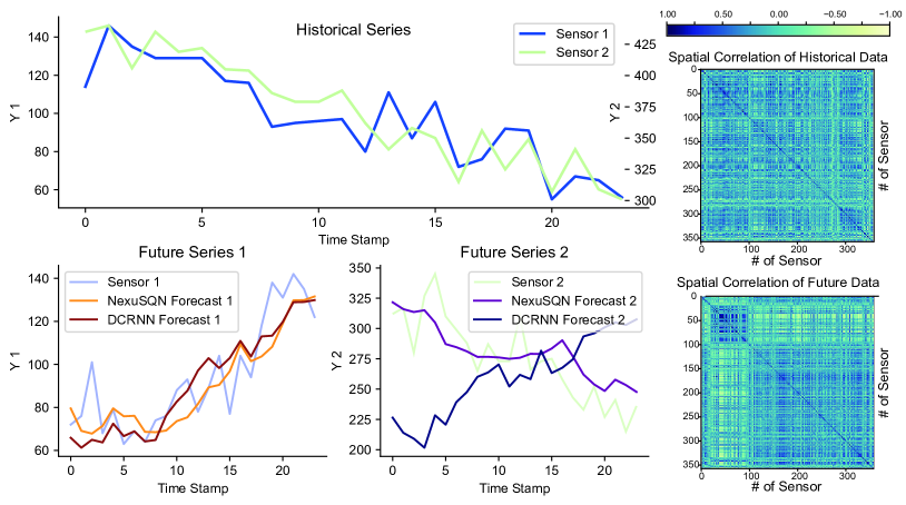
Figure 2. Spatial contextualization issue.

4.6. Benefits of Parsimonious Models

Based on the minimalist MLP-Mixer structure, NexuSQN features both accuracy, efficiency and flexibility. The additional benefits of a parsimonious model are evident in the following paragraphs.

High Computational Efficiency

Fig. 3 (a) shows the validation MAE curves of several competing STGNNs on traffic speed data. Fig 3 (b) details the training speed, model size, and memory usage. It is worth noting that NexuSQN exhibits significantly faster training speed, with convergence achieved in just 10 minutes of GPU time. Moreover, it has a smoother convergence curve, a lower error bound, and requires less training expense, indicating high efficiency and scalability. This superiority is achieved through a combination of a technically simple architecture, linear model complexity, and parameter-efficient designs. Advanced STGNNs like DGCRN and D2STGNN apply alternating GNNs and temporal models, resulting in high computational burdens and unstable optimization.

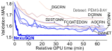
(a) Convergency curves

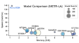
(b) Model efficiency

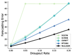
(c) Model robustness

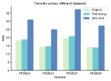
(d) Model transferability

Figure 3. Benefits of simple models.

Robustness Under Attack

Fig. 3 (c) displays the forecasting errors after randomly corrupting some proportions of weight parameters in the input or readout layer. As can be seen, NexuSQN is more robust than complicated ones when faced with external attack.

Flexibility to Transfer

NexuSQN can easily be transferred by resorting to the learnable node embedding. In Fig. 3 (d), we train NexuSQN on PEMS08 data and only fine-tune the node embedding on other datasets. We find that the fine-tuning of embedding performs comparably with the models trained from scratch.

5. Deployed Applications

Existing models for STDF have been extensively validated on public benchmarks, but their effectiveness in large-scale urban road networks and real-world production environments has been less studied. Therefore, we deploy our model in real-world challenges and showcase its practical applications in two testing stages.

5.1. Stage 1: Scalability in Offline Pre-training

The scalability of the proposed NexuSQN was tested in an Urban Congestion Project (UCP). In UCP, a vast database containing 27,070 taxis with more than 900 million vehicle trajectories was collected and desensitized. This database was collected from various taxi companies, covering the primary road networks of Beijing, Shanghai, and Shenzhen cities in China. The raw trajectory database was processed using the map-matching algorithm (Brakatsoulas et al., 2005) and the average speeds were calculated. We then aggregated the speed values into three grid-based datasets with a 300-m resolution in Tab. 12.

Table 12. Statistics of private urban traffic datasets.

Datasets	Range	Data points	Grids	Vehicles
Beijing	115.7°-117.4° E, 39.4°-41.6° N	270 million	8,267	12,060
Shenzhen	113.5°-114.4° E, 22.3°-22.5° N	210 million	7,680	6,330
Shanghai	120.5°-122.1° E, 30.4°-31.5° N	420 million	8,854	8,680

To investigate the temporal evolution and spatial propagation of traffic congestion at the regional level, deep learning models were trained on an offline server. These models used the three large-scale urban datasets to forecast the traffic speed across the entire network. The regional and network-level forecasts of NexuSQN deployed on our internal server are shown in Fig. 4. Full results are given in Tab. 17. Many advanced STGNNs and Transformers adopt computational-intensive techniques. As a consequence, the high dimensionality of urban networks made many of them fail to respond promptly on a single computing server. In contrast, NexuSQN completed the pre-training task with high efficiency and achieved greater accuracy than other baselines.

(a) Traffic forecast at network level (Beijing and Shanghai)

(b) Traffic forecast at regional level (Shanghai)

Figure 4. Scalability demonstrations.

5.2. Stage 2: Feasibility in Online Parallel Testing

In this testing phase, we collaborated with Baidu to conduct an online parallel test in Baoding and Yizhuang districts. The aim of the test was to examine the feasibility of the models in generating fine-grained real-time congestion maps in real-world production environments. The architecture of the system is shown in Fig. 5.

For each test instance, we fine-tuned pretrained models from stage 1 using data from the first month of 2023 in Baoding and Yizhuang datasets. Then the online data streaming was synchronous for all instances and model inference was carried out in each parallel computing server. To meet the requirement of real-time query using Baidu Map’s API, traffic data flow was updated every 3 minutes and models need to forecast the online stream. The test results were displayed on the online dashboard, as shown in Fig. 5. With high data throughput ($>25$ batch/s), NexuSQN generated results in real time, e.g., 87.7 s in Baoding data. Due to the delay in data transmission, many STGNNs with high complexity could not complete the real-time testing task in limited execution times. Compared to other testing models like Autoformer, NexuSQN showed significant improvements. It achieved over 15% higher accuracy in generating traffic state maps and over 20 times faster online inference speed. Overall, the testing phase demonstrated the efficiency and effectiveness of our model in production environments.

Figure 5. Online testing system architecture and results.

6. Conclusion and Outlook

This paper extends the MLP-Mixers in large-scale urban data forecasting problems. By addressing spatiotemporal contextualization issues in a simple yet effective way, we demonstrate a scalable contextualized MLP-Mixer called NexuSQN. NexuSQN customizes structured time and space mixing operations with learnable embedding. Extensive evaluations show that NexuSQN performs on par with advanced STGNNs and Transformers with high computational efficiency. It also has the potential to model and analyze general spatiotemporal data in urban systems. We also deploy it in a real-world urban congestion project and present its practical applications. Future work could deploy it on edge computing devices and achieve online model training. It could also be combined with distributed techniques to achieve privacy-preserving purposes.

Appendix

In this technical appendix, we provide additional details on experimental setups, model implementations, and related works. In addition, supplementary evaluation results and case studies are provided for additional discussion.

Appendix A Detailed Experimental Setups

This section provides additional information about the adopted datasets, baseline models, and detailed experimental settings for the results presented in the main paper.

A.1. Dataset Descriptions

We adopt several public urban computing datasets to benchmark our model. They include traffic flow, environmental measurements, and energy records, which are widely used in relevant studies.

Traffic Flow Benchmarks

(1) To evaluate the short-term forecasting performance, we adopt six high-resolution highway traffic flow datasets, including two traffic speed datasets: METR-LA and PEMS-BAY  (Li et al., 2018), and four traffic volume datasets: PEMS03, PEMS04, PEMS07, and PEMS08 (Guo et al., 2021). The six datasets contain traffic measurements aggregated every 5 minutes from loop sensors installed on highway networks. METR-LA contains spot speed data from 207 loop sensors over a period of 4 months from Mar 2012 to Jun 2012, located at the Los Angeles County highway network. PEMS-BAY records 6 months of speed data from $325$ static detectors in the San Francisco South Bay Area. PEMS0X contains the real-time highway traffic volume information in California, collected by the Caltrans Performance Measurement System (PeMS) (Chen et al., 2001) in every 30 seconds. The raw traffic flow is aggregated into a 5-minute interval for the experiments. Similarly to METR-LA and PEMS-BAY, PEMS0X also includes an adjacency graph calculated by the physical distance between the sensors. (2) To evaluate NexuSQN’s long-term forecasting performance, we use the TrafficL benchmark (Lai et al., 2018). This dataset provides hourly records of road occupancy rates (between 0 and 1) measured by 862 sensors on San Francisco Bay Area freeways over a period of 48 months. (3) To verify the scalability of models, we adopt the large-scale LargeST benchmarks. LargeST dataset contains 5 years of traffic readings from 01/01/2017 to 12/31/2021 collected every 5 minutes by 8600 traffic sensors in California. We adopt the largest subset GLA and use the readings from 2019 that are considered, aggregated into 15-minute intervals for experiments.

Air Quality Benchmarks

AQI data from the Urban Air project (Zheng et al., 2015) record PM2.5 pollutant measurements collected by 437 air quality monitoring stations across 43 Chinese cities from May 2014 to April 2015 with an aggregation interval of 1 hour. Note that AQI data contains nearly $26\%$ missing data.

Energy Production and Consumption Benchmarks

Large-scale PU-VS production data (Hummon et al., 2012) consists of a simulated energy production by 5016 PV farms in the United States during 2006. The original observations are aggregated into a 30-minute window. Electricity benchmark is widely adopted to evaluate long-term forecast performance. It records load profiles (in kWh) measured hourly by 321 sensors from 2012 to 2014. CER-En: smart meters measuring energy consumption from the Irish Commission for Energy Regulation Smart Metering Project . Following (Cini et al., 2022), we consider the full sensor network containing 6435 smart meters with a 30-minute aggregation interval.

Global Meteorological Benchmarks

Global Wind and Global Temp (Wu et al., 2023b) contain the hourly averaged wind speed and hourly temperature of meteorological 3850 stations around the world from 1 January 2019 to 31 December 2020 from the National Centers for Environmental Information (NCEI) system.

A.2. Experimental Setups

Table 13. Input and output settings.

Datasets		window	Horizon	Graphs
Traffic	METR-LA	12	12	True
	PEMS-BAY	12	12	True
	PEMS03	12	12	True
	PEMS04	12	12	True
	PEMS07	12	12	True
	PEMS08	12	12	True
	TrafficL	96	384	False
	LargeST-GLA	12	12	True
Energy	Electricity	336	96	False
	CER-EN	36	22	True
	PV-US	36	22	True
Environ.	AQI	24	3	True
	Global Temp	48	24	False
	Global Wind	48	24	False

Basic Setups

We adopt the widely used input-output settings in related literature to evaluate the models. These settings are given in Tab. 13. For all the datasets, we adopt the same training (70%), validating (10%), and testing (20%) set splits and preprocessing steps as previous work. It is worth commenting that NexuSQN does not rely on redefined graphs, and results in Tab. 10 indicate that the benefits of incorporating predefined graphs are marginal. Time-of-day information is provided as exogenous variables for our model, and day-of-week feature is input to baselines that require this information. In addition, labels with nonzero values are used to compute the metrics. And the performance of all methods is recorded in the same evaluation environment. We evaluate the model’s performance using metrics such as mean absolute error (MAE), mean squared error (MSE), and mean absolute percentage error (MAPE). For long-term benchmarks including TrafficL and Electricity, we do not use the standardization on labels and use the normalized mean absolute error (NMAE), mean relative error (MRE), and mean absolute percentage error (MAPE) as metrics.

Ablation Study

We consider the following three variations:

• w $\mathbf{A}_{\text{pre}}$: We add additional diffusion graph convolutions (Li et al., 2018) with three forward and backward diffusion steps using distance-based graphs in SpaceMixer.

• w/o SpaceMixer: We remove the “SpaceMixer” design by keeping each channel independent (Nie et al., 2022). In this scenario, our model shares a structure similar to that of STID (Shao et al., 2022a).

• w/o $\mathbf{E}_{T}$: We remove the spatiotemporal node embedding, and our model degrades into a spatiotemporal Mlp-Mixer (Chen et al., 2023).

For each of them, we keep the same experimental settings in Section 4 and report the forecasting results.

Robustness Study

To evaluate the robustness under model attack, we select several representative STGNNs and randomly corrupt a proportion of linear weights in the input embedding or the final readout layer. These corrupted values are filled with zeros.

Transfer Study

As suggested in (Cini et al., 2023b), node embedding can facilitate transfer between different datasets. Therefore, we first pretrain our model on small PEMS08 data, then freeze all parameters except node embedding. During the transfer stage, we randomly initialize the node embedding according to the spatial dimension of the target larger datasets (i.e., PEMS03, PEMS04, and PEMS07) and fine tune the embedding parameter.

Table 14. Hyperparameters of NexuSQN.

Model configurations		PEMS03	PEMS04	PEMS07	PEMS08
Hyperparameter	input_emb_size	128	128	128	128
	n_spacemixer	1	1	1	1
	activation	GeLU
	st_embed	False	True	True	False
	node_emb_size	64	64	64	96
Training configs	window_size	12
	horizon	12
	batch_size	32
	learning_rate	0.005
	lr_gamma	0.1
	lr_milestones	[40,60]

Model configurations		METR-LA	PEMS-BAY	TrafficL	LargeST
Hyperparameter	input_emb_size	48	64	128	128
	n_spacemixer	1	1	2	1
	activation	GeLU
	st_embed	False	False	False	False
	node_emb_size	80	96	64	96
Training configs	window_size	12		96	12
	horizon	12		384	12
	batch_size	32	32	16	16
	learning_rate	0.005
	lr_gamma	0.1
	lr_milestones	[20,30,40]

Appendix B Reproducibility

In order to ensure the reproducibility of this paper, this sections provides the detailed implementations of NexuSQN, as a technical complement to the descriptions presented in the paper. Our code to reproduce the reported results is available at https://github.com/tongnie/NexuSQN.

Platform

All these experiments are conducted on a Windows platform with one single NVIDIA RTX A6000 GPU with 48GB memory. Our implementations and suggested hyperparameters are mainly based on PyTorch (Paszke et al., 2019), Torch Spatiotemporal (Cini and Marisca, 2022), and BasicTS (Shao et al., 2023) benchmarking tools.

Hyperparameters

To ensure a fair and unbiased comparison, we adopt the original implementations presented in each paper. We also use the recommended hyperparameters for the baselines wherever possible. During evaluation, all baselines are trained, validated, and tested in identical environments. Our NexuSQN contains only a few model hyperparameters and is easy to tune. The detailed configurations of traffic datasets are shown in Tab. 14. And the hyperparameters of other datasets can be found in our repository. The configurations of other baseline models and implementations follow the official resources as much as possible.

Table 15. Full results on METR-LA, PEMS-BAY, PEMS03, PEMS04, PEMS07, and PEMS08 datasets. MAE for {15, 30, 60} minutes forecasting horizons, as well as MAE, MSE, and MAPE averaged over one hour (12 time steps) are reported.

Dataset	METR-LA						PEMS-BAY						PEMS03
Metric	15 min	30 min	60 min	Average			15 min	30 min	60 min	Average			15 min	30 min	60 min	Average
	MAE	MAE	MAE	MAE	MSE	MAPE (%)	MAE	MAE	MAE	MAE	MSE	MAPE (%)	MAE	MAE	MAE	MAE	MAPE (%)
AGCRN	2.85	3.19	3.56	3.14	40.94	8.69	1.38	1.69	1.94	1.63	13.59	3.71	14.65	15.72	16.82	15.58	15.08
DCRNN	2.81	3.23	3.75	3.20	41.12	8.90	1.37	1.72	2.09	1.67	14.52	3.78	14.59	15.76	18.18	15.90	15.74
GWNet	2.74	3.14	3.58	3.09	38.86	8.52	1.31	1.65	1.96	1.59	13.31	3.57	13.67	14.60	16.23	14.66	14.88
GatedGN	2.72	3.05	3.43	3.01	37.19	8.20	1.34	1.65	1.92	1.58	13.17	3.55	13.72	15.49	19.08	17.08	14.44
GRUGCN	2.93	3.47	4.24	3.46	48.47	9.85	1.39	1.81	2.30	1.77	16.70	4.03	14.63	16.44	19.87	16.62	15.96
EvolveGCN	3.27	3.82	4.59	3.81	52.64	10.56	1.53	2.00	2.53	1.95	18.98	4.43	17.07	19.03	22.22	19.11	18.61
ST-Transformer	2.97	3.53	4.34	3.52	51.49	10.06	1.39	1.81	2.29	1.77	17.01	4.09	14.03	15.72	18.74	15.85	15.37
STGCN	2.84	3.25	3.80	3.23	40.34	9.02	1.37	1.71	2.08	1.66	14.11	3.75	14.27	15.49	18.02	15.61	16.07
STID	2.82	3.18	3.56	3.13	41.83	9.07	1.32	1.64	1.93	1.58	13.05	3.58	13.88	15.26	17.41	15.27	16.39
MTGNN	2.79	3.12	3.46	3.07	39.91	8.57	1.34	1.65	1.91	1.58	13.52	3.51	13.74	14.76	16.13	14.70	14.90
D2STGNN	2.74	3.08	3.47	3.05	38.30	8.44	1.30	1.60	1.89	1.55	12.94	3.50	13.36	14.45	15.96	14.45	14.55
DGCRN	2.73	3.10	3.54	3.07	39.02	8.39	1.33	1.65	1.95	1.59	13.12	3.61	13.83	14.77	16.14	14.73	14.86
SCINet	3.06	3.47	4.09	3.47	44.61	9.93	1.52	1.85	2.24	1.82	14.92	4.14	14.39	15.25	17.37	15.43	15.37
NexuSQN	2.66	2.99	3.36	2.95	35.35	8.04	1.30	1.60	1.86	1.54	12.42	3.45	13.15	14.20	15.79	14.18	13.77

Dataset	PEMS04					PEMS07					PEMS08
Metric	15 min	30 min	60 min	Average		15 min	30 min	60 min	Average		15 min	30 min	60 min	Average
	MAE	MAE	MAE	MAE	MAPE (%)	MAE	MAE	MAE	MAE	MAPE (%)	MAE	MAE	MAE	MAE	MAPE (%)
AGCRN	18.27	18.95	19.83	18.90	12.69	19.55	20.65	22.40	20.64	9.42	14.50	15.16	16.41	15.23	10.46
DCRNN	19.19	20.54	23.55	20.75	14.32	20.47	22.11	25.77	22.30	9.51	14.84	15.93	18.22	16.06	10.40
GWNet	18.17	18.96	20.23	18.95	13.59	19.87	20.97	23.53	21.13	9.96	14.21	14.99	16.45	15.02	9.70
GatedGN	18.10	18.84	20.03	18.81	13.11	21.01	22.74	25.81	22.68	10.18	14.07	14.96	16.27	14.91	9.64
GRUGCN	19.89	22.28	27.37	22.68	15.81	21.15	24.00	29.91	24.37	10.29	15.46	17.32	21.16	17.55	11.43
EvolveGCN	23.21	25.82	30.97	26.21	17.79	24.72	28.09	34.41	28.40	12.11	18.21	20.46	24.45	20.64	13.11
ST-Transformer	19.13	21.33	25.69	21.63	15.12	20.17	22.80	27.74	23.05	9.77	14.39	15.87	18.69	16.00	10.71
STGCN	19.26	20.75	24.03	20.95	14.79	20.26	22.33	26.58	22.53	9.66	14.81	16.02	18.76	16.20	10.57
STID	17.77	18.60	20.01	18.60	12.87	18.66	19.93	21.91	19.88	8.82	13.53	14.29	15.75	14.32	9.69
MTGNN	17.88	18.49	19.62	18.48	12.76	18.94	20.23	22.23	20.19	8.59	13.80	14.57	15.82	14.57	9.46
D2STGNN	17.60	18.39	19.63	18.39	12.65	18.49	20.74	23.10	20.84	9.99	13.65	14.53	16.00	14.52	9.40
DGCRN	18.05	18.76	20.07	18.77	13.13	18.58	21.10	22.55	21.24	10.45	13.96	14.68	15.96	14.70	9.62
SCINet	18.30	19.03	20.85	19.19	13.31	21.63	22.89	25.96	23.11	10.00	14.57	15.60	17.75	15.77	10.13
NexuSQN	17.37	18.05	19.14	18.03	12.34	18.15	19.34	21.05	19.28	8.05	13.17	13.96	15.28	13.98	9.02

• - Best results are bold marked. Note that - indicates the model runs out of memory with the minimum batch size.

Appendix C Supplementary Results

Full Results of Traffic Data

Full results of short-term traffic benchmarks including the MAE at {3,6,12} steps are given in Tab. 15.

Full Results of Efficiency Analysis

Full results of computational performance on METR-LA and PEMS-BAY data are shown in Tab. 16. And additional illustrations are given in Figs. 6 and 7.

Table 16. Model computational performances.

	METR-LA				PEMS-BAY
	Speed (Batch/s)	Memory (GB)	Batch size	Model size (k)	Speed (Batch/s)	Memory (GB)	Batch size	Model size (k)
AGCRN	10.43	4.1	64	989	6.78	6.0	64	991
DCRNN	9.90	3.8	64	387	6.72	5.5	64	387
GWNet	10.50	3.4	64	301	7.11	5.0	64	303
GatedGN	13.53	6.0	32	74.6	11.27	7.1	16	82.2
ST-Transformer	5.77	8.2	64	236	6.63	7.6	32	236
STGCN	17.31	2.9	64	194	12.05	3.8	64	194
MTGNN	21.39	2.9	64	405	13.54	4.9	64	573
D2STGNN	5.02	6.9	32	392	5.38	7.0	16	394
DGCRN	2.82	8.0	64	199	2.74	6.9	32	208
NexuSQN	137.35	1.2	64	60.5	90.26	1.3	64	75.6

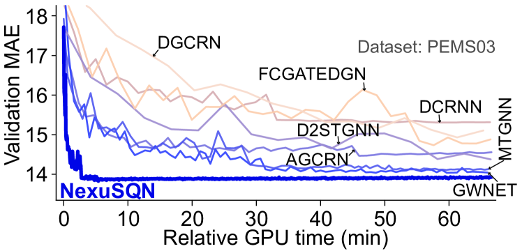
Figure 6. Validation MAE curves of different models.

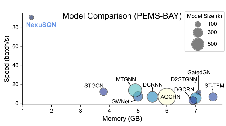
Figure 7. Computational performance.

Case Study on Temporal Contextualization

An illustration of the temporal contextualization issue and the behavior of different models is provided in Fig. 8.

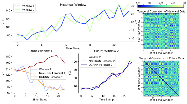
Figure 8. Temporal contextualization issue.

Table 17. Results on Baoding, Yizhuang, Beijing, Shenzhen and Shanghai urban traffic data. (192 to 192)

	Baoding		Yizhuang		Beijing		Shenzhen		Shanghai
	MAE	WAPE	MAE	WAPE	MAE	WAPE	MAE	WAPE	MAE	WAPE
MTGNN	13.66	59.55	16.41	77.20	OOM	OOM	22.38	55.91	OOM	OOM
AGCRN	OOM	OOM	12.24	59.61	OOM	OOM	OOM	OOM	OOM	OOM
StemGNN	12.34	55.59	12.97	61.16	OOM	OOM	OOM	OOM	OOM	OOM
TimesNet	10.12	48.77	11.78	56.60	15.52	45.69	18.22	45.37	16.39	40.88
Pyraformer	8.42	37.92	10.86	51.05	OOM	OOM	OOM	OOM	OOM	OOM
Autoformer	9.09	40.94	11.55	54.31	17.47	47.11	21.22	52.67	17.75	45.07
FEDformer	8.44	37.87	10.06	47.33	17.69	47.72	22.25	55.21	18.10	45.96
Informer	8.36	37.68	10.91	49.59	17.37	46.83	21.23	52.71	17.09	43.39
DLinear	8.65	38.76	10.71	50.36	13.69	36.92	13.61	37.79	13.48	34.24
PatchTST	9.99	44.98	10.53	49.52	13.62	36.74	14.55	36.11	12.95	32.89
NexuSQN	7.89	35.54	9.55	44.91	11.21	30.23	10.89	32.01	11.03	27.98

Additional Results on Private data

Full evaluation results in five private data are shown in Tab. 17. The models are trained or fine-tuned to forecast the future 192 steps using the historical 192 steps. Online parallel testing results are given in Fig. 9.

Figure 9. Online testing results of NexuSQN.

Appendix D Additional Interpretations

To give a clear exposition of the design concept of our model, we provide more discussions and interpretations on the model architecture and the connections with related works in this section.

D.1. Additional Architecture Details

Time Stamp Encoding

We adopt sinusoidal positional encoding to inject the time-of-day information along time dimension:

(15) $$PE_{\text{sine}} =\texttt{sin}(p_{i}*2\pi/\delta_{D}),$$

$$PE_{\text{cosine}} =\texttt{cos}(p_{i}*2\pi/\delta_{D}),$$

$$\mathbf{U}_{t} =\left[PE_{\text{sine}}\|PE_{\text{cosine}}\right],$$

where $p_{i}$ is the index of $i$-th time point in the series, and $\delta_{D}$ is the day-unit time mapping. We concatenate $PE_{\text{sine}}$ and $PE_{\text{cosine}}$ as the final temporal encoding. In fact, day-of-week embedding can also be applied using the one-hot encoding.

Node Embedding

For the spatial dimension, we adopt a unique identifier for each sensor. While an optional structural embedding is the random-walk diffusion matrix (Dwivedi et al., 2020), for simplicity, we use the learnable node embedding (Shao et al., 2022a) as a simple index positional encoding without any structural priors. Learnable node embedding can be easily implemented by initializing a parameter with its gradient trackable, i.e.,

⬇

self.emb = nn.Parameter(

Tensor(self.num_nodes, self.emb_size),

requires_grad=True)

The initialization method (e.g., Gaussian or uniform distribution) can be used to specify its initial distribution.

Dense Readout

For a multi-step STDF task, we adopt a Mlp and a reshaping layer to directly output the predictions:

(16) $$\widehat{\mathbf{X}}_{T+1:T+H}=\textsc{Mlp}(\mathbf{H}^{(L+1)}),$$

$$\widehat{\mathcal{X}}_{T+1:T+H}=\texttt{UNFOLD}(\widehat{\mathbf{X}}_{T+1:T+H}),$$

where $\texttt{UNFOLD}(\cdot)$ is the inverse linear operator of $\texttt{FOLD}(\cdot)$. For simplicity, we avoid a complex sequential decoder and directly make multi-step predictions through regression.

Interpretations of the Temporal Contextualization Issue

Different from the spatial contextualization issue, the temporal contextualization issue can be shown in a typical linear predictive model with weight $\mathbf{W}$ and bias $\mathbf{b}$, expressed as follows:

(17) $$\mathbf{x}_{t+1:t+H}=\mathbf{W}\mathbf{x}_{t-W:t}+\mathbf{b},$$

or: $$x_{t+h}=\sum_{k=0}^{W}w_{k,h}x_{t-k}+b_{k,h},~{}h\in\{1,\dots,H\}.$$

Eq. (17) is an autoregressive model (AR) for each forecast horizon. Its weight $w_{k,h}$ depends solely on the relative time order and is agnostic to the absolute position in the sequence, rendering it incapable of contextualizing the series in temporal dimension. In this case, the temporal context is needed.

In the discussion by (Chen et al., 2023), predictive models like Eq. (17) are referred to as time-dependent. An upgrade to this type is termed data-dependent, where the weight becomes pattern-aware and conditions on temporal variations:

(18) $$x_{t+h}=\sum_{k=0}^{W}\mathcal{F}_{k}(\mathbf{x}_{t-W:t})x_{t-k}+b_{k,h},$$

where $\mathcal{F}_{k}(\cdot)$ represents a data-driven function, such as self-attention. Eq. (18) creates a fully time-varying AR process, which is parameterized by time-varying coefficients (Bringmann et al., 2017). However, its overparameterization can lead to overfitting of the data, rather than capturing the temporal relationships, such as the position on the time axis.

D.2. Remarks on Parameter-Efficient Designs

The proposed scalable mixing layers have several parameter-efficient designs. As NexuSQN conducts space mixing only after one time mixing rather than at every time point, it is more efficient than alternately stacking spatial-temporal blocks. We introduce these techniques and explain how they lighten the model structure.

Residual Connection

In each block, we incorporate a shortcut for the linear part. When all residual connections are activated (e.g., when spatial modeling is unnecessary), NexuSQN can degrade into a family of channel-independent linear models. This feature makes it promising for long-term series forecasting tasks (Zeng et al., 2022; Das et al., 2023).

Parameter Sharing

In contrast to recent design trends that use separate node parameters or graphs for different layers (Zhang et al., 2020; Oreshkin et al., 2021), we use a globally shared node embedding for all modules, including the TimeMixer and SpaceMixer. This aims to simplify the end-to-end training of random embedding while reducing the model size. Furthermore, Yang et al. (2022) and Han et al. (2022) showed that MLP and GNN can share similar feature spaces. Without the contextualization function, SpaceMixer can collapse into TimeMixer. Considering this, we instantiate consecutive SpaceMixer layers with a shared feedforward weight. This parameter-sharing design is inspired by the connection between MLP and GNN in spatiotemporal graphs.

Shallow-Layer Structure

Instead of using deep multilayer architectures, we use shallow layer structures with larger receptive fields. Specifically, we adopt a small number of structured space mixing layers (e.g., 1 layer in most cases) with all-to-all connections to capture long-range interactions. This approach avoids the use of multiple stacking of sparse graph aggregators or hierarchical operations such as diffusion convolutions (Li et al., 2018). This treatment is consistent with the previous finding that wider graphs can be more expressive than deeper ones under some conditions (Wu et al., 2023a). In other words, when the graph is dense, a single global mixing can gather adequate information adaptively from arbitrary nodes. Therefore, despite the simple structure, it has sufficient expressivity and a large receptive field to capture pairwise interactions. Another crucial aspect to consider when utilizing an all-to-all connection is that it prompts the model to gather comprehensive information from other windows to obtain a precise “temporal context.”

D.3. Connections with Related Works

This detailed section on related work highlights recent advances in simplified neural forecasting models and advanced embedding techniques. We aim to provide a nexus between notable achievements by offering a meticulous exposition of two primary research avenues: (1) simplified models for time series forecasting; and (2) node embedding for spatiotemporal data, the unification of which served as the catalyst for driving the development of this work.

Simplified Models for Time Series Forecasting

Within the literature on time series studies, long-term series forecasting (LTSF) is considered one of the most challenging tasks. Encouragingly, recent studies have revisited the design of neural architectures and sought a simpler solution for this long-standing topic and empirically show the superiority of simple models over their complex counterparts, especially using the MLP-based architectures (Zeng et al., 2022; Zhang et al., 2022; Das et al., 2023; Chen et al., 2023). In particular, Zeng et al. (2022) analyzed the ineffectiveness of Transformer-based models on this task and outperformed an array of advanced Transformer-based baselines with a family of linear models. N-BEATS (Oreshkin et al., 2019) and H-HITS (Challu et al., 2023) combine multiscale learning with residual MLP structures for univariate forecasting. Chen et al. (2023) developed a fully MLP model that performs mixing operations along both the time and the feature dimensions, called TSMixer. The cross-sensor information is utilized by a weighted sum of all series. TiDE proposed by (Das et al., 2023) enjoys a dense encoder-decoder structure with a residual MLP backbone. FreTS (Yi et al., 2023), PITS (Lee et al., 2023) and MSD-Mixer (Zhong et al., 2023) further incorporate elaborate inductive biases into the MLP structures and have shown improved performance. Note that the channel-independence design in DLinear (Zeng et al., 2022), TiDE (Das et al., 2023) and PatchTST (Nie et al., 2022) makes the model a global univariate one. While the channel mixing in (Chen et al., 2023; Zhang et al., 2022) implicitly models the multivariate relationships between series.

However, investigations into the short-term spatiotemporal data forecasting are still lacking. The studied STDF differs from LTSF in two ways: (1) complex temporal patterns (e.g., nonstationary) with higher resolution; (2) subtle interaction between multivariate series. Therefore, we conjecture that the emerging Transformers-like or MLP-based models designed for LTSF may be less effective in the context of spatiotemporal data, as the above methods basically adopt a channel-independence assumption and ignore the explicit spatial correlations between series (Zeng et al., 2022; Das et al., 2023). To adapt to the spatiotemporal case, several pioneering works have attempted to simplify the neural forecasting architectures in different aspects. In particular, Cini et al. (2022) proposed a scalable graph predictor based on the random-walk diffusion and the echo-state network to encode spatiotemporal representations prior to model training. Liu et al. (2023b) developed two alternative spatial techniques including a pre-processing-based ego graph method and a global sensor embedding to model spatial correlations. The processed spatial features are further fed to temporal models such as RNNs, TCNs, and WaveNets. A graph sampling strategy is required to improve training performance. However, both approaches rely on complex temporal encoders and precomputed graph features, which can cause high complexity in engineering applications. Zhang et al. (2023) and Wang et al. (2023) extend MLP-Mixers in spatiotemporal traffic forecasting problems and demonstrate their effectiveness and efficiency. These findings prompt us to further explore the MLP-Mixer paradigm.

Node Embedding for Spatiotemporal Data

Node embedding or positional encoding in the graph machine learning domain is a commonly used technique to enhance the expressive power of GNNs (Dwivedi et al., 2022). However, methodologies and applications in spatiotemporal graph modeling have been relatively limited. In this line of research, Deng et al. (2021) identify the bottleneck of deep forecasting models as ineffective in distinguishing high-frequency components from input signals. A spatiotemporal normalization scheme is proposed to enhance the WaveNet models. Shao et al. (2022a) discuss the spatiotemporal identification problem and propose to assign a learnable embedding for each node and time step in a MLP structure. In contrast to the focus of these efforts, we focus on the spatiotemporal contextualization problems posed by the mixing operation in the canonical MLP-Mixer model rather than the data itself. Furthermore, GatedGN model proposed in (Satorras et al., 2022) follows a time-then-graph template and considers the node index as a static identifier. Global attention is used to infer the latent graphs. However, all pairwise attention with time complexity $\mathcal{O}(N^{2})$ is computationally expensive. More recently, Cini et al. (2023b) interpreted the role of node embedding as local effects in global models and provided a systematic framework for incorporating it into different architectures. Several regularization and transfer learning strategies are also discussed.

Building upon existing work, our work lies at the crossroads of these two research trajectories. We leverage these advances and extend the MLP-Mixer architecture for large-scale urban data. We also showcase its practical applications and deployments.

References

- (1)
- Bai et al. (2020) Lei Bai, Lina Yao, Can Li, Xianzhi Wang, and Can Wang. 2020. Adaptive graph convolutional recurrent network for traffic forecasting. Advances in neural information processing systems 33 (2020), 17804–17815.
- Brakatsoulas et al. (2005) Sotiris Brakatsoulas, Dieter Pfoser, Randall Salas, and Carola Wenk. 2005. On map-matching vehicle tracking data. In Proceedings of the 31st international conference on Very large data bases. 853–864.
- Bringmann et al. (2017) Laura F Bringmann, Ellen L Hamaker, Daniel E Vigo, André Aubert, Denny Borsboom, and Francis Tuerlinckx. 2017. Changing dynamics: Time-varying autoregressive models using generalized additive modeling. Psychological methods 22, 3 (2017), 409.
- Cao et al. (2020) Defu Cao, Yujing Wang, Juanyong Duan, Ce Zhang, Xia Zhu, Congrui Huang, Yunhai Tong, Bixiong Xu, Jing Bai, Jie Tong, et al. 2020. Spectral temporal graph neural network for multivariate time-series forecasting. Advances in neural information processing systems 33 (2020), 17766–17778.
- Challu et al. (2023) Cristian Challu, Kin G Olivares, Boris N Oreshkin, Federico Garza Ramirez, Max Mergenthaler Canseco, and Artur Dubrawski. 2023. Nhits: Neural hierarchical interpolation for time series forecasting. In Proceedings of the AAAI Conference on Artificial Intelligence, Vol. 37. 6989–6997.
- Chen et al. (2001) Chao Chen, Karl Petty, Alexander Skabardonis, Pravin Varaiya, and Zhanfeng Jia. 2001. Freeway performance measurement system: mining loop detector data. Transportation Research Record 1748, 1 (2001), 96–102.
- Chen et al. (2023) Si-An Chen, Chun-Liang Li, Nate Yoder, Sercan O Arik, and Tomas Pfister. 2023. Tsmixer: An all-mlp architecture for time series forecasting. arXiv preprint arXiv:2303.06053 (2023).
- Cini and Marisca (2022) Andrea Cini and Ivan Marisca. 2022. Torch Spatiotemporal. https://github.com/TorchSpatiotemporal/tsl
- Cini et al. (2022) Andrea Cini, Ivan Marisca, Filippo Maria Bianchi, and Cesare Alippi. 2022. Scalable Spatiotemporal Graph Neural Networks. arXiv preprint arXiv:2209.06520 (2022).
- Cini et al. (2023a) Andrea Cini, Ivan Marisca, Daniele Zambon, and Cesare Alippi. 2023a. Graph Deep Learning for Time Series Forecasting. arXiv preprint arXiv:2310.15978 (2023).
- Cini et al. (2023b) Andrea Cini, Ivan Marisca, Daniele Zambon, and Cesare Alippi. 2023b. Taming Local Effects in Graph-based Spatiotemporal Forecasting. arXiv preprint arXiv:2302.04071 (2023).
- Das et al. (2023) Abhimanyu Das, Weihao Kong, Andrew Leach, Rajat Sen, and Rose Yu. 2023. Long-term Forecasting with TiDE: Time-series Dense Encoder. arXiv preprint arXiv:2304.08424 (2023).
- Deng et al. (2021) Jinliang Deng, Xiusi Chen, Renhe Jiang, Xuan Song, and Ivor W Tsang. 2021. St-norm: Spatial and temporal normalization for multi-variate time series forecasting. In Proceedings of the 27th ACM SIGKDD conference on knowledge discovery & data mining. 269–278.
- Dwivedi et al. (2020) Vijay Prakash Dwivedi, Chaitanya K Joshi, Anh Tuan Luu, Thomas Laurent, Yoshua Bengio, and Xavier Bresson. 2020. Benchmarking graph neural networks. arXiv preprint arXiv:2003.00982 (2020).
- Dwivedi et al. (2022) Vijay Prakash Dwivedi, Anh Tuan Luu, Thomas Laurent, Yoshua Bengio, and Xavier Bresson. 2022. Graph Neural Networks with Learnable Structural and Positional Representations. In International Conference on Learning Representations. https://openreview.net/forum?id=wTTjnvGphYj
- Elsayed et al. (2021) Shereen Elsayed, Daniela Thyssens, Ahmed Rashed, Hadi Samer Jomaa, and Lars Schmidt-Thieme. 2021. Do we really need deep learning models for time series forecasting? arXiv preprint arXiv:2101.02118 (2021).
- Fusco et al. (2022) Francesco Fusco, Damian Pascual, and Peter Staar. 2022. pNLP-mixer: an efficient all-MLP architecture for language. arXiv preprint arXiv:2202.04350 (2022).
- Gao and Ribeiro (2022) Jianfei Gao and Bruno Ribeiro. 2022. On the Equivalence Between Temporal and Static Equivariant Graph Representations. In International Conference on Machine Learning. PMLR, 7052–7076.
- Guo et al. (2019) Shengnan Guo, Youfang Lin, Ning Feng, Chao Song, and Huaiyu Wan. 2019. Attention based spatial-temporal graph convolutional networks for traffic flow forecasting. In Proceedings of the AAAI Conference on Artificial Intelligence, Vol. 33. 922–929.
- Guo et al. (2021) Shengnan Guo, Youfang Lin, Huaiyu Wan, Xiucheng Li, and Gao Cong. 2021. Learning dynamics and heterogeneity of spatial-temporal graph data for traffic forecasting. IEEE Transactions on Knowledge and Data Engineering 34, 11 (2021), 5415–5428.
- Han et al. (2022) Xiaotian Han, Tong Zhao, Yozen Liu, Xia Hu, and Neil Shah. 2022. MLPInit: Embarrassingly Simple GNN Training Acceleration with MLP Initialization. arXiv preprint arXiv:2210.00102 (2022).
- He et al. (2023) Xiaoxin He, Bryan Hooi, Thomas Laurent, Adam Perold, Yann LeCun, and Xavier Bresson. 2023. A generalization of vit/mlp-mixer to graphs. In International Conference on Machine Learning. PMLR, 12724–12745.
- Hummon et al. (2012) Marissa Hummon, Eduardo Ibanez, Gregory Brinkman, and Debra Lew. 2012. Sub-hour solar data for power system modeling from static spatial variability analysis. Technical Report. National Renewable Energy Lab.(NREL), Golden, CO (United States).
- Jin et al. (2023) Ming Jin, Huan Yee Koh, Qingsong Wen, Daniele Zambon, Cesare Alippi, Geoffrey I Webb, Irwin King, and Shirui Pan. 2023. A Survey on Graph Neural Networks for Time Series: Forecasting, Classification, Imputation, and Anomaly Detection. arXiv preprint arXiv:2307.03759 (2023).
- Lai et al. (2018) Guokun Lai, Wei-Cheng Chang, Yiming Yang, and Hanxiao Liu. 2018. Modeling long-and short-term temporal patterns with deep neural networks. In The 41st international ACM SIGIR conference on research & development in information retrieval. 95–104.
- Lee et al. (2023) Seunghan Lee, Taeyoung Park, and Kibok Lee. 2023. Learning to Embed Time Series Patches Independently. arXiv preprint arXiv:2312.16427 (2023).
- Li et al. (2023) Fuxian Li, Jie Feng, Huan Yan, Guangyin Jin, Fan Yang, Funing Sun, Depeng Jin, and Yong Li. 2023. Dynamic graph convolutional recurrent network for traffic prediction: Benchmark and solution. ACM Transactions on Knowledge Discovery from Data 17, 1 (2023), 1–21.
- Li et al. (2018) Yaguang Li, Rose Yu, Cyrus Shahabi, and Yan Liu. 2018. Diffusion Convolutional Recurrent Neural Network: Data-Driven Traffic Forecasting. In International Conference on Learning Representations.
- Liu et al. (2022b) Minhao Liu, Ailing Zeng, Muxi Chen, Zhijian Xu, Qiuxia Lai, Lingna Ma, and Qiang Xu. 2022b. Scinet: Time series modeling and forecasting with sample convolution and interaction. Advances in Neural Information Processing Systems 35 (2022), 5816–5828.
- Liu et al. (2022a) Shizhan Liu, Hang Yu, Cong Liao, Jianguo Li, Weiyao Lin, Alex X. Liu, and Schahram Dustdar. 2022a. Pyraformer: Low-Complexity Pyramidal Attention for Long-Range Time Series Modeling and Forecasting. In International Conference on Learning Representations. https://openreview.net/forum?id=0EXmFzUn5I
- Liu et al. (2023b) Xu Liu, Yuxuan Liang, Chao Huang, Hengchang Hu, Yushi Cao, Bryan Hooi, and Roger Zimmermann. 2023b. Do We Really Need Graph Neural Networks for Traffic Forecasting? arXiv preprint arXiv:2301.12603 (2023).
- Liu et al. (2023c) Xu Liu, Yutong Xia, Yuxuan Liang, Junfeng Hu, Yiwei Wang, Lei Bai, Chao Huang, Zhenguang Liu, Bryan Hooi, and Roger Zimmermann. 2023c. LargeST: A Benchmark Dataset for Large-Scale Traffic Forecasting. arXiv preprint arXiv:2306.08259 (2023).
- Liu et al. (2023a) Yong Liu, Tengge Hu, Haoran Zhang, Haixu Wu, Shiyu Wang, Lintao Ma, and Mingsheng Long. 2023a. itransformer: Inverted transformers are effective for time series forecasting. arXiv preprint arXiv:2310.06625 (2023).
- Nie et al. (2023a) Tong Nie, Guoyang Qin, Yunpeng Wang, and Jian Sun. 2023a. Correlating sparse sensing for large-scale traffic speed estimation: A Laplacian-enhanced low-rank tensor kriging approach. Transportation Research Part C: Emerging Technologies 152 (2023), 104190.
- Nie et al. (2023b) Tong Nie, Guoyang Qin, Yunpeng Wang, and Jian Sun. 2023b. Towards better traffic volume estimation: Tackling both underdetermined and non-equilibrium problems via a correlation adaptive graph convolution network. arXiv preprint arXiv:2303.05660 (2023).
- Nie et al. (2022) Yuqi Nie, Nam H Nguyen, Phanwadee Sinthong, and Jayant Kalagnanam. 2022. A Time Series is Worth 64 Words: Long-term Forecasting with Transformers. arXiv preprint arXiv:2211.14730 (2022).
- Oreshkin et al. (2021) Boris N Oreshkin, Arezou Amini, Lucy Coyle, and Mark Coates. 2021. FC-GAGA: Fully connected gated graph architecture for spatio-temporal traffic forecasting. In Proceedings of the AAAI Conference on Artificial Intelligence, Vol. 35. 9233–9241.
- Oreshkin et al. (2019) Boris N Oreshkin, Dmitri Carpov, Nicolas Chapados, and Yoshua Bengio. 2019. N-BEATS: Neural basis expansion analysis for interpretable time series forecasting. arXiv preprint arXiv:1905.10437 (2019).
- Pareja et al. (2020) Aldo Pareja, Giacomo Domeniconi, Jie Chen, Tengfei Ma, Toyotaro Suzumura, Hiroki Kanezashi, Tim Kaler, Tao Schardl, and Charles Leiserson. 2020. Evolvegcn: Evolving graph convolutional networks for dynamic graphs. In Proceedings of the AAAI conference on artificial intelligence, Vol. 34. 5363–5370.
- Paszke et al. (2019) Adam Paszke, Sam Gross, Francisco Massa, Adam Lerer, James Bradbury, Gregory Chanan, Trevor Killeen, Zeming Lin, Natalia Gimelshein, Luca Antiga, et al. 2019. Pytorch: An imperative style, high-performance deep learning library. Advances in neural information processing systems 32 (2019), 8026–8037.
- Satorras et al. (2022) Victor Garcia Satorras, Syama Sundar Rangapuram, and Tim Januschowski. 2022. Multivariate Time Series Forecasting with Latent Graph Inference. arXiv preprint arXiv:2203.03423 (2022).
- Shao et al. (2023) Zezhi Shao, Fei Wang, Yongjun Xu, Wei Wei, Chengqing Yu, Zhao Zhang, Di Yao, Guangyin Jin, Xin Cao, Gao Cong, et al. 2023. Exploring Progress in Multivariate Time Series Forecasting: Comprehensive Benchmarking and Heterogeneity Analysis. arXiv preprint arXiv:2310.06119 (2023).
- Shao et al. (2022a) Zezhi Shao, Zhao Zhang, Fei Wang, Wei Wei, and Yongjun Xu. 2022a. Spatial-Temporal Identity: A Simple yet Effective Baseline for Multivariate Time Series Forecasting. In Proceedings of the 31st ACM International Conference on Information & Knowledge Management. 4454–4458.
- Shao et al. (2022b) Zezhi Shao, Zhao Zhang, Wei Wei, Fei Wang, Yongjun Xu, Xin Cao, and Christian S Jensen. 2022b. Decoupled dynamic spatial-temporal graph neural network for traffic forecasting. arXiv preprint arXiv:2206.09112 (2022).
- Srinivasan and Ribeiro (2019) Balasubramaniam Srinivasan and Bruno Ribeiro. 2019. On the equivalence between positional node embeddings and structural graph representations. arXiv preprint arXiv:1910.00452 (2019).
- Tolstikhin et al. (2021) Ilya O Tolstikhin, Neil Houlsby, Alexander Kolesnikov, Lucas Beyer, Xiaohua Zhai, Thomas Unterthiner, Jessica Yung, Andreas Steiner, Daniel Keysers, Jakob Uszkoreit, et al. 2021. Mlp-mixer: An all-mlp architecture for vision. Advances in neural information processing systems 34 (2021), 24261–24272.
- Tsai et al. (2019) Yao-Hung Hubert Tsai, Shaojie Bai, Makoto Yamada, Louis-Philippe Morency, and Ruslan Salakhutdinov. 2019. Transformer dissection: a unified understanding of transformer’s attention via the lens of kernel. arXiv preprint arXiv:1908.11775 (2019).
- Vaswani et al. (2017) Ashish Vaswani, Noam Shazeer, Niki Parmar, Jakob Uszkoreit, Llion Jones, Aidan N Gomez, Łukasz Kaiser, and Illia Polosukhin. 2017. Attention is all you need. In Advances in neural information processing systems. 5998–6008.
- Wang et al. (2023) Zepu Wang, Yuqi Nie, Peng Sun, Nam H Nguyen, John Mulvey, and H Vincent Poor. 2023. St-mlp: A cascaded spatio-temporal linear framework with channel-independence strategy for traffic forecasting. arXiv preprint arXiv:2308.07496 (2023).
- Wu et al. (2022) Haixu Wu, Tengge Hu, Yong Liu, Hang Zhou, Jianmin Wang, and Mingsheng Long. 2022. TimesNet: Temporal 2D-Variation Modeling for General Time Series Analysis. arXiv preprint arXiv:2210.02186 (2022).
- Wu et al. (2021) Haixu Wu, Jiehui Xu, Jianmin Wang, and Mingsheng Long. 2021. Autoformer: Decomposition transformers with auto-correlation for long-term series forecasting. Advances in Neural Information Processing Systems 34 (2021), 22419–22430.
- Wu et al. (2023b) Haixu Wu, Hang Zhou, Mingsheng Long, and Jianmin Wang. 2023b. Interpretable weather forecasting for worldwide stations with a unified deep model. Nature Machine Intelligence (2023), 1–10.
- Wu et al. (2023a) Qitian Wu, Wentao Zhao, Chenxiao Yang, Hengrui Zhang, Fan Nie, Haitian Jiang, Yatao Bian, and Junchi Yan. 2023a. Simplifying and Empowering Transformers for Large-Graph Representations. arXiv preprint arXiv:2306.10759 (2023).
- Wu et al. (2020) Zonghan Wu, Shirui Pan, Guodong Long, Jing Jiang, Xiaojun Chang, and Chengqi Zhang. 2020. Connecting the Dots: Multivariate Time Series Forecasting with Graph Neural Networks. In Proceedings of the 26th ACM SIGKDD International Conference on Knowledge Discovery and Data Mining. Association for Computing Machinery, New York, NY, USA, 753–763.
- Wu et al. (2019) Zonghan Wu, Shirui Pan, Guodong Long, Jing Jiang, and Chengqi Zhang. 2019. Graph Wavenet for Deep Spatial-Temporal Graph Modeling. In Proceedings of the 28th International Joint Conference on Artificial Intelligence. 1907–1913.
- Xu et al. (2020) Mingxing Xu, Wenrui Dai, Chunmiao Liu, Xing Gao, Weiyao Lin, Guo-Jun Qi, and Hongkai Xiong. 2020. Spatial-temporal transformer networks for traffic flow forecasting. arXiv preprint arXiv:2001.02908 (2020).
- Yang et al. (2022) Chenxiao Yang, Qitian Wu, Jiahua Wang, and Junchi Yan. 2022. Graph Neural Networks are Inherently Good Generalizers: Insights by Bridging GNNs and MLPs. arXiv preprint arXiv:2212.09034 (2022).
- Yi et al. (2023) Kun Yi, Qi Zhang, Wei Fan, Shoujin Wang, Pengyang Wang, Hui He, Defu Lian, Ning An, Longbing Cao, and Zhendong Niu. 2023. Frequency-domain MLPs are More Effective Learners in Time Series Forecasting. arXiv preprint arXiv:2311.06184 (2023).
- Yu et al. (2018) Bing Yu, Haoteng Yin, and Zhanxing Zhu. 2018. Spatio-temporal graph convolutional networks: a deep learning framework for traffic forecasting. In Proceedings of the 27th International Joint Conference on Artificial Intelligence. 3634–3640.
- Zeng et al. (2022) Ailing Zeng, Muxi Chen, Lei Zhang, and Qiang Xu. 2022. Are transformers effective for time series forecasting? arXiv preprint arXiv:2205.13504 (2022).
- Zhang et al. (2020) Qi Zhang, Jianlong Chang, Gaofeng Meng, Shiming Xiang, and Chunhong Pan. 2020. Spatio-temporal graph structure learning for traffic forecasting. In Proceedings of the AAAI conference on artificial intelligence, Vol. 34. 1177–1185.
- Zhang et al. (2022) Tianping Zhang, Yizhuo Zhang, Wei Cao, Jiang Bian, Xiaohan Yi, Shun Zheng, and Jian Li. 2022. Less is more: Fast multivariate time series forecasting with light sampling-oriented mlp structures. arXiv preprint arXiv:2207.01186 (2022).
- Zhang et al. (2023) Zijian Zhang, Ze Huang, Zhiwei Hu, Xiangyu Zhao, Wanyu Wang, Zitao Liu, Junbo Zhang, S Joe Qin, and Hongwei Zhao. 2023. MLPST: MLP is All You Need for Spatio-Temporal Prediction. In Proceedings of the 32nd ACM International Conference on Information and Knowledge Management. 3381–3390.
- Zheng et al. (2020) Chuanpan Zheng, Xiaoliang Fan, Cheng Wang, and Jianzhong Qi. 2020. Gman: A graph multi-attention network for traffic prediction. In Proceedings of the AAAI Conference on Artificial Intelligence, Vol. 34. 1234–1241.
- Zheng et al. (2015) Yu Zheng, Xiuwen Yi, Ming Li, Ruiyuan Li, Zhangqing Shan, Eric Chang, and Tianrui Li. 2015. Forecasting fine-grained air quality based on big data. In Proceedings of the 21th ACM SIGKDD international conference on knowledge discovery and data mining. 2267–2276.
- Zhong et al. (2023) Shuhan Zhong, Sizhe Song, Guanyao Li, Weipeng Zhuo, Yang Liu, and S-H Gary Chan. 2023. A multi-scale decomposition mlp-mixer for time series analysis. arXiv preprint arXiv:2310.11959 (2023).
- Zhou et al. (2021) Haoyi Zhou, Shanghang Zhang, Jieqi Peng, Shuai Zhang, Jianxin Li, Hui Xiong, and Wancai Zhang. 2021. Informer: Beyond efficient transformer for long sequence time-series forecasting. In Proceedings of the AAAI conference on artificial intelligence, Vol. 35. 11106–11115.
- Zhou et al. (2022) Tian Zhou, Ziqing Ma, Qingsong Wen, Xue Wang, Liang Sun, and Rong Jin. 2022. Fedformer: Frequency enhanced decomposed transformer for long-term series forecasting. In International Conference on Machine Learning. PMLR, 27268–27286.