Equivalence, Identity, and Unitarity Checking in Black-Box Testing of Quantum Programs

Abstract

Quantum programs exhibit inherent non-deterministic behavior, which poses more significant challenges for error discovery compared to classical programs. While several testing methods have been proposed for quantum programs, they often overlook fundamental questions in black-box testing. In this paper, we bridge this gap by presenting three novel algorithms specifically designed to address the challenges of equivalence, identity, and unitarity checking in black-box testing of quantum programs. We also explore optimization techniques for these algorithms, including specialized versions for equivalence and unitarity checking, and provide valuable insights into parameter selection to maximize performance and effectiveness. To evaluate the effectiveness of our proposed methods, we conducted comprehensive experimental evaluations, which demonstrate that our methods can rigorously perform equivalence, identity, and unitarity checking, offering robust support for black-box testing of quantum programs.

1 Introduction

Quantum computing, which utilizes the principles of quantum mechanics to process information and perform computational tasks, is a rapidly growing field with the potential to revolutionize various disciplines [37]. It holds promise for advancements in optimization [15], encryption [36], machine learning [6], chemistry [30], and materials science [49]. Quantum algorithms, when compared to classical algorithms, offer the potential to accelerate the solution of specific problems [13, 22, 40]. As quantum hardware devices and algorithms continue to develop, the importance of creating high-quality quantum software has become increasingly evident. However, the nature of quantum programs, with their special characteristics such as superposition, entanglement, and non-cloning theorems, makes it challenging to track errors in these programs [34, 27]. Therefore, effective testing of quantum programs is crucial for the advancement of quantum software development.

Black-box testing [5] is a software testing method that assesses the functionality of a program without examining its internal structure or implementation details. This method has broad applications for identifying software errors and improving software reliability. The inherently non-deterministic behavior of quantum programs makes error detection more challenging than in classical programs. Additionally, due to the potential interference of measurement with quantum states, observing the internal behavior of quantum programs becomes nearly impossible. Consequently, black-box testing assumes a crucial role in testing quantum programs. While several testing methods for quantum programs have been proposed [1, 2, 17, 28, 33, 43], these methods have paid limited attention to the fundamental questions in black-box testing of quantum programs. Important questions essential to black-box testing for quantum programs have remained largely unexplored.

Black-box testing of quantum programs refers to testing these programs based solely on selecting the appropriate inputs and detecting the corresponding outputs. To effectively address the challenges associated with black-box testing in quantum programs, it is essential to explore and answer the following fundamental research questions (RQs):

• Equivalence Checking: Given two quantum programs $\mathcal{P}$ and $\mathcal{P^{\prime}}$, how can we determine whether they are equivalent?

• Identity Checking: Given a quantum program $\mathcal{P}$, how can we check whether it represents an identity transform?

• Unitarity Checking: Given a quantum program $\mathcal{P}$, how can we ascertain whether it represents a unitary transform?

In this paper, we aim to address these RQs and lay the foundation for black-box testing of quantum programs. We propose three novel methods that specifically target equivalence, identity, and unitarity checking in quantum programs. For equivalence checking, we introduce a novel method based on the Swap Test, which compares the outputs of two quantum programs on Pauli input states. To simplify identity checking, we present a straightforward approach to avoid repeated running. Additionally, we derive a critical theorem that provides a necessary and sufficient condition for a quantum operation to be a unitary transform, enabling us to develop an effective unitarity checking method.

Furthermore, we conduct theoretical analyses and experimental evaluations to demonstrate the effectiveness and efficiency of our proposed methods. The results of our evaluations confirm that our methods successfully perform equivalence, identity, and unitarity checking, supporting the black-box testing of quantum programs.

In summary, our paper makes the following contributions:

• A theorem on unitarity checking: We proved a critical theorem about how to check whether a quantum operation is a unitary transform, which is a basis for developing our algorithm for unitarity checking.

• Checking algorithms: We develop three novel algorithms for checking the equivalence, identity, and unitarity of quantum programs, respectively.

• Algorithm optimization: We explore the optimization of our checking algorithms by devising optimized versions that specifically target equivalence and unitarity checking. We also discuss and provide detailed insights into the selection of algorithm parameters to maximize their performance and effectiveness.

• Experimental evaluation: We evaluate the effectiveness of our methods from experimental perspectives. The evaluation results show that our methods can effectively perform the equivalence, identity, and unitarity checking to support the black-box testing of quantum programs.

Through these contributions, our paper advances the foundation of black-box testing for quantum programs and provides valuable insights for quantum software development.

The organization of this paper is as follows. Section 2 introduces some basic concepts and technologies of quantum computation. We discuss questions and their motivations we want to address in this paper in Section 3. Section 4 presents novel algorithms to solve these questions. Section 5 discusses the optimization of equivalence checking and unitarity checking. Section 6 discusses the experimental evaluation. Section 7 discusses the threats to the validity of our methods. We discuss related works in Section 8, and the conclusion is given in Section 9.

2 Background

We next introduce some background knowledge about quantum computation which is necessary for understanding the content of this paper.

2.1 Basic Concepts of Quantum Computation

A qubit is the basis of quantum computation. Like the classical bit has values 0 and 1, a qubit also has two basis states with the form $\left|0\right>$ and $\left|1\right>$ and can contain a superposition between basis states. The general state of a qubit is $a\left|0\right>+b\left|1\right>$, where $a$ and $b$ are two complex numbers called amplitudes that satisfy $|a|^{2}+|b|^{2}=1$. The basis states are similar to binary strings for more than one qubit. For example, a two-qubit system has four basis states: $\left|00\right>$, $\left|01\right>$, $\left|10\right>$ and $\left|11\right>$, and the general state is $a_{00}\left|00\right>+a_{01}\left|01\right>+a_{10}\left|10\right>+a_{11}\left|11\right>$, where $|a_{00}|^{2}+|a_{01}|^{2}+|a_{10}|^{2}+|a_{11}|^{2}=1$. The state can also be written as a column vector $[a_{00},a_{01},a_{10},a_{11}]^{T}$, which is called state vector. Generally, the quantum state on $n$ qubits can be represented as a state vector in Hilbert space of $d$ dimension, where $d=2^{n}$.

The states mentioned above are all pure states, which means they are not probabilistic. Sometimes a quantum system may have a probability distribution over several pure states rather than a certain state, which we call a mixed state. Suppose a quantum system is in state $\left|\psi_{i}\right>$ with probability $p_{i}$. The completeness of probability gives that $\sum_{i}p_{i}=1$. We can denote the mixed state as the ensemble representation: $\{(p_{i},\left|\psi_{i}\right>)\}$.

Besides state vectors, the density operator or density matrix is another way to express a quantum state, which is convenient for expressing mixed states. Suppose a mixed state has the ensemble representation $\{(p_{i},\left|\psi_{i}\right>)\}$, the density operator of this state is $\rho=\sum_{i}p_{i}\left|\psi_{i}\right>\left<\psi_{i}\right|$, where $\left<\psi_{i}\right|$ is the conjugate transpose of $\left|\psi_{i}\right>$ (thus it is a row vector and $\left|\psi_{i}\right>\left<\psi_{i}\right|$ is a $d\times d$ matrix). The density operator of a pure state $\left|\phi\right>$ is $\left|\phi\right>\left<\phi\right|$. Owing that the probability $p_{i}\geq 0$ and $\sum_{i}p_{i}=1$, a lawful and complete density operator $\rho$ should satisfy: (1) $tr(\rho)=1$ and (2) $\rho$ is a positive operator. $\rho$ represents a pure state if and only if $tr(\rho^{2})=1$ [38].

2.2 Evolution of Quantum States

Quantum computing is performed by applying proper quantum gates on qubits. An $n$-qubit quantum gate can be represented by a $2^{n}\times 2^{n}$ unitary matrix $G$. Applying gate $G$ on a state vector $\left|\psi\right>$ will obtain state $G\left|\psi\right>$. Moreover, applying $G$ on a density operator will obtain state $G\rho G^{\dagger}$, where $G^{\dagger}$ is the conjugate transpose of $G$. For a unitary transform, $G^{\dagger}=G^{-1}$, where $G^{-1}$ is the inverse of $G$. There are several basic quantum gates, such as single-qubit gates $X$, $Z$, $S$, $H$, and two-qubit gate CNOT. The matrices of them are:

$$X=\left[\begin{array}[]{cc}0&1\\ 1&0\end{array}\right],\quad Z=\left[\begin{array}[]{cc}1&0\\ 0&-1\end{array}\right],\quad S=\left[\begin{array}[]{cc}1&0\\ 0&i\end{array}\right],$$

$$H=\frac{1}{\sqrt{2}}\left[\begin{array}[]{cc}1&1\\ 1&-1\end{array}\right],\quad\mathrm{CNOT}=\left[\begin{array}[]{cccc}1&0&0&0\\ 0&1&0&0\\ 0&0&0&1\\ 0&0&1&0\end{array}\right]$$

In quantum devices, the information of qubits can only be obtained by measurement. Measuring a quantum system will get a classical value with the probability of corresponding amplitude. Then the state of the quantum system will collapse into a basis state according to obtained value. For example, measuring a qubit $a\left|0\right>+b\left|1\right>$ will get result 0 and collapse into state $\left|0\right>$ with probability $|a|^{2}$ and get result 1 and collapse into state $\left|1\right>$ with probability $|b|^{2}$. This property brings uncertainty and influences the testing of quantum programs.

A quantum circuit is a popular model to express the process of quantum computing. Every line represents a qubit in a quantum circuit model, and a sequence of operations is applied from left to right. Figures 2 and 2 are two examples of quantum circuits.

2.3 Quantum Operations and Quantum Programs

Quantum operation is a general mathematical model of state transformation, which can describe the general evolution of a quantum system [38]. Suppose we have an input density operator $\rho$ ($d\times d$ matrix); after an evolution through quantum operation $\mathcal{E}$, the density operator becomes $\mathcal{E}(\rho)$. $\mathcal{E}(\rho)$ can be represented as the operator-sum representation [38]: $\mathcal{E}(\rho)=\sum_{i}E_{i}\rho E_{i}^{\dagger}$, where $E_{i}$ is $d\times d$ matrix. If $\sum_{i}E_{i}^{\dagger}E_{i}=I$, then $\mathcal{E}$ is called a trace-preserving quantum operation.

In developing quantum programs, programmers use quantum gates, measurements, and control statements to implement some quantum algorithms. A quantum program usually transforms the quantum input state into another state. An important fact is that a quantum program with if statements and while-loop statements, where the if and while-loop conditions can contain the result of measuring qubits, can be represented by a quantum operation [32]. So quantum operations formalism is a powerful tool that can be used by our testing methods to model the state transformations of quantum programs under test. In addition, a program will eventually terminate if and only if it corresponds to a trace-preserving quantum operation [32]. This paper focuses only on trace-preserving quantum operations, i.e., the quantum programs that always terminate.

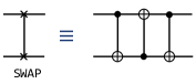
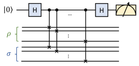
Figure 1: A SWAP gate that can be implemented by three CNOT gates.

Figure 2: The quantum circuit of Swap Test.

2.4 Swap Test

The Swap Test [7, 3] is a procedure in quantum computation that allows us to determine how similar two quantum states are. Figure 2 shows the quantum circuit of the Swap Test. It includes two registers carrying the states $\rho$ and $\sigma$ and an ancillary qubit initialized in state $\left|0\right>$. It contains a series of "controlled-SWAP" gates on each pair of corresponding qubits of target states $\rho$ and $\sigma$, and the ancilla qubit is used for controlling. SWAP gate can be implemented as three CNOT gates as shown in Figure 2. The ancilla qubit is measured at the end, and the probability that result 1 occurs, denoted as $p_{1}$, is related to states $\rho$ and $\sigma$ as shown in the following formula (1):

$$tr(\rho\sigma)=1-2p_{1}$$ (1)

Note that the probability $p_{1}$ can be estimated by repeating running the Swap Test and counting the proportion of obtaining result 1. Based on this process, we can estimate parameter $tr(\rho\sigma)$ and then obtain more useful information on states $\rho$ and $\sigma$. In particular, if we set $\sigma=\rho$, we can estimate $tr(\rho^{2})$ and use it to determine whether $\rho$ is a pure or mixed state. Also, if we let $\rho$ and $\sigma$ be two pure states, where $\rho=\left|\alpha\right>\left<\alpha\right|$ and $\sigma=\left|\beta\right>\left<\beta\right|$, then we have $tr(\rho\sigma)=\left|\left<\alpha|\beta\right>\right|^{2}$, where $\left<\alpha|\beta\right>$ represents the inner product of two state $\left|\alpha\right>$ and $\left|\beta\right>$. We call $\left|\alpha\right>$ and $\left|\beta\right>$ are orthogonal, denoted as $\left|\alpha\right>\bot\left|\beta\right>$, if $\left<\alpha|\beta\right>=0$.

2.5 Quantum Tomography

Quantum tomography [12] is used for obtaining the details of a quantum state or operation. Because measurement may collapse a quantum state, we need many copies of the target quantum state or repeat the target quantum operation many times to reconstruct the target. State tomography reconstructs the information of a quantum state, and process tomography reconstructs the information of a quantum operation.

In quantum tomography, The following four Pauli matrices are important:

$$\sigma_{0}=\left[\begin{array}[]{cc}1&0\\ 0&1\end{array}\right],\qquad\sigma_{1}=\left[\begin{array}[]{cc}0&1\\ 1&0\end{array}\right],$$

$$\sigma_{2}=\left[\begin{array}[]{cc}0&-i\\ i&0\end{array}\right],\qquad\sigma_{3}=\left[\begin{array}[]{cc}1&0\\ 0&-1\end{array}\right]$$

All $\sigma_{1}$, $\sigma_{2}$ and $\sigma_{3}$ have two eigenvalues: $-1$ and $1$. $\sigma_{3}$ has eigenstates $\left|0\right>=[1,0]^{T}$ (for eigenvalue $1$) and $\left|1\right>=[0,1]^{T}$ (for eigenvalue $-1$). $\sigma_{1}$ has eigenstates $\left|+\right>=\frac{1}{\sqrt{2}}(\left|0\right>+\left|1\right>)$ (for $1$) and $\left|-\right>=\frac{1}{\sqrt{2}}(\left|0\right>-\left|1\right>)$ (for $-1$). $\sigma_{2}$ has eigenstates $\left|+_{i}\right>=\frac{1}{\sqrt{2}}(\left|0\right>+i\left|1\right>)$ (for $1$) and $\left|-_{i}\right>=\frac{1}{\sqrt{2}}(\left|0\right>-i\left|1\right>)$ (for $-1$). $\sigma_{0}$ has only one eigenvalue $1$, and any single-qubit state is its eigenstate.

Note that the four Pauli matrices form a group of bases of the space of the single-qubit density operator. Similarly, the tensor product of Pauli matrices $\sigma_{\vec{v}}=\sigma_{v_{1}}\otimes\sigma_{v_{2}}\otimes\cdots\otimes\sigma_{v_{n}}$ form a basis of an $n$-qubit density operator, where $v_{i}\in\{0,1,2,3\}$, $\vec{v}=(v_{1},\dots,v_{n})$. A density operator $\rho$ can be represented by Pauli basis [38]:

$$\rho=\sum_{\vec{v}}\frac{tr(\sigma_{\vec{v}}\rho)}{2^{n}}\sigma_{\vec{v}}$$ (2)

where each $tr(\sigma_{\vec{v}}\rho)$ can be obtained by Pauli measurement of Pauli matrix $\sigma_{\vec{v}}$. We can conduct experiments to observe each $tr(\sigma_{\vec{v}}\rho)$ on $\rho$ and then use formula (2) to reconstruct the density operator of $\rho$.

A quantum operation $\mathcal{E}$ is a linear transformation on the input space, so it depends on the behavior of a group of bases. We can use state tomography to reconstruct the corresponding output density operators of all basis input states, and then $\mathcal{E}$ can be reconstructed by these output density operators [38].

3 Questions and Motivations

We next outline the key questions addressed in this paper and provide a comprehensive rationale for each question, supported by relevant scenarios. By doing so, we aim to highlight the motivation and necessity behind investigating these specific aspects.

3.1 Modelling Black-Box Quantum Programs

In this paper, we focus on black-box testing, where we do not require prior knowledge of the internal structure of the target program. Instead, we achieve the testing objective by observing the program’s outputs when provided with suitable inputs. This approach allows us to evaluate the program’s behavior without relying on specific implementation details.

The beginning of our discussion is to model a black-box quantum program. In [2], Ali et al. gives some definitions of a quantum program, input, output, and program specification to guide the generation of test cases. They define the program specification as the expected probability distribution of the classical output values under the given inputs. As [29] points out, this definition is inherently classical and implies that the program is ended with measurements to transform quantum information into classical probabilities. It is more reasonable to deal directly with quantum information rather than transform them into classical probabilities. Accordingly, the quantum input and output of the program can be modeled by quantum states (state vectors or density operators).

According to Section 2.2, a quantum program with if statements and while-loop statements can be represented by a quantum operation [32]. So in this paper, we use the quantum operation model to represent a black-box quantum program. A black-box quantum program with quantum input variable $\rho$ can be represented by an unknown quantum operation $\mathcal{E}$, and $\mathcal{E}(\rho)$ represents the corresponding output under input $\rho$. The research on the properties of quantum programs can be transformed into research on quantum operations.

3.2 Questions

We introduce the key questions addressed in this paper, namely equivalence checking, identity checking, and unitarity checking. While a quantum program can involve classical inputs and outputs, our focus in this paper is solely on the quantum aspects. Specifically, we aim to examine the checking of quantum inputs and outputs while keeping other classical parameters fixed. We outline the three questions addressed in this paper as follows:

Question 1

Equivalence Checking

Given two quantum programs $\mathcal{P}_{1}$ and $\mathcal{P}_{2}$, how can we determine whether they are equivalent, meaning they produce the same quantum output for the same quantum input?

Question 2

Identity Checking Given a quantum program $\mathcal{P}$, how can we check whether it represents an identity transform where the input qubits remain unchanged?

Question 3

Unitarity Checking

Given a quantum program $\mathcal{P}$, how can we determine whether $\mathcal{P}$ represents a unitary transform?

3.3 Motivations

Next, we discuss the motivation and necessity of each question. We will present several scenarios that highlight the practical application of equivalence, identity, and unitary checking in the context of black-boxing testing of quantum programs.

The equivalence of the two programs holds substantial importance, as it is a prevalent relationship. Even when testing classical programs, checking the equivalence of two programs is a fundamental testing task. For instance, in the following Scenario 1, one of the typical applications of equivalence checking is to guarantee the correctness of an updated program version.

Scenario 1

Correctness Assurance in Version Update

One important application of equivalence checking is to ensure the correctness of an updated version of a quantum program in regression testing. Let us consider a scenario where we have an original program $\mathcal{P}$, and after a few months, we develop an updated version $\mathcal{P^{\prime}}$ by making improvements such as optimizing the program’s structure to enhance its execution speed. In this case, ensuring that these modifications do not alter the program’s behavior becomes crucial, meaning that $\mathcal{P^{\prime}}$ should be equivalent to $\mathcal{P}$. By performing an equivalence checking, we can verify if the updated version $\mathcal{P^{\prime}}$ maintains the same functionality as the original version $\mathcal{P}$.

It seems that we need to test all possible quantum inputs to check, and the number of quantum inputs is uncountable. Fortunately, the linearity of quantum operations allows us to check only a finite subset of all inputs. Moreover, our task is to test rather than rigorously prove. Therefore, we only need to select small and suitable test cases to check.

Unlike equivalence checking, identity checking and unitarity checking reflect the properties of quantum programs. There is no classical counterpart to unitarity checking, and the classical counterpart to identity checking - checking whether a classical program outputs its input - is meaningless. Identity checking makes sense in testing quantum programs because implementing a reverse variant of the original quantum program is common in quantum programming. The behavior of many quantum programs is to perform a unitary transformation of the quantum input state. According to Section 2.2, any unitary transformation $U$ has an inverse $U^{-1}$ and they have the relation $UU^{-1}=I$, where $I$ is the identity transformation. As shown in Scenario 2, identity checking can be used to test the inverse variant of the original quantum program.

Scenario 2

Testing the Inverse Variant

Suppose we have completed a testing task for an original program P. Now, we proceed to implement the reverse version invP of P. While some quantum programming languages, such as Q#[41] and isQ[23], offer mechanisms for generating invP automatically, these mechanisms come with some restrictions on the target program. For instance, if P contains if statements associated with classical input parameters, the quantum behavior of P is a unitary transform for any fixed classical parameters, implying the existence of the inverse invP. However, these languages may not have the ability to automatically generate invP as their mechanisms are limited to dealing with simple programs. In such cases, manual implementation is required. As a result, effective testing becomes crucial during the manual implementation process.

To test invP, as proposed in [29], we only need to check the following relation:

$\texttt{P}\circ\texttt{invP}=I$

where ’$\circ$’ represents the sequential execution (from right to left) of the two subroutines. This task involves checking the identity relationship between the composed and identity programs ($I$).

Besides the inverse variant, as mentioned in [29], there are also two other variants of an original program P - controlled variants CtrlP and power variants PowP. For example, the testing process for power variants can be reduced to check the following relations:

For $k>0$, $\texttt{InvP}^{k}\circ\texttt{PowP}(k)=I$;

For $k<0$, $\texttt{P}^{|k|}\circ\texttt{PowP}(k)=I$.

The motivation for unitarity checking is based on the fact that many practical quantum programs are unitary transformations, which means that they do not contain measurements. If the unitarity checking fails for these programs, we can know that there exist some unexpected measurements in them. Scenario 3 gives another case where we need to employ unitarity checking.

Scenario 3

Checking the Program Specification

Checking whether the program output conforms to the program specification is a crucial step in testing. However, unlike classical programs, where the output can be directly observed, checking the output of quantum programs under arbitrary inputs can be challenging. Fortunately, as discussed in [29], if the intended behavior of the program is to perform a unitary transform, we can simplify the checking process. It involves checking (1) the output under classical input states and (2) performing additional unitarity checking on the program.

4 Checking Algorithms

We next introduce concrete checking algorithms to solve these questions mentioned in Section 3. For each algorithm, we discuss the theoretical basis first and then give concrete algorithms. We denote $n$ as the number of qubits of target programs.

4.1 Implementation of Swap Test

First, we discuss the implementation of the Swap Test. The quantum circuit for the Swap Test is shown in Figure 2. According to the formula (1), a useful parameter is the probability of returning result 1. So our implementation returns the number of occurrences of result 1, with a given number of repeat $s$ of the Swap Test. The initial states $\rho,\sigma$ are generated by two input subroutines $\mathcal{P}_{1}$ and $\mathcal{P}_{2}$.

The implementation of the Swap Test is shown in Algorithm 1. Lines $3\sim 5$ initialize quantum variables and prepare the input states by $\mathcal{P}_{1}$ and $\mathcal{P}_{2}$; lines $6\sim 8$ implement a series of controlled-SWAP operations. Line $10$ measures the ancilla qubit, and lines $11\sim 13$ accumulate the number of results 1. The time complexity of Algorithm 1 is $O(ns)$, and it requires $2n+1$ qubits.

Input: ($n$, $s$, $\mathcal{P}_{1}$, $\mathcal{P}_{2}$)

 $n$: the number of qubits of one target state;

 $s$: the number of rounds;

 $\mathcal{P}_{1},\mathcal{P}_{2}$: two subroutines to generate two target states.

Output: $s_{1}$: Number of occurrences of result 1.

1

2$s_{1}\leftarrow 0$;

3 for i = 1 to $s$ do

4       qanc $\leftarrow\left|0\right>$; qs1 $\leftarrow\left|0\right>^{\otimes n}$; qs2 $\leftarrow\left|0\right>^{\otimes n}$;

5       $H(\textbf{qanc})$;

6       $\mathcal{P}_{1}(\textbf{qs1})$; $\mathcal{P}_{2}(\textbf{qs2})$;

7       for j = 0 to $n-1$ do

8             Controlled SWAP(qanc, (qs1[j], qs2[j]));

9            

10       end for

11      $H(\textbf{qanc})$;

12       $m\leftarrow$ Measure(qanc);

13       if $m=1$ then

14            $s_{1}\leftarrow s_{1}+1$;

15       end if

16      

17 end for

18return $s_{1}$;

Algorithm 1 SwapTest

4.2 Equivalence Checking

A straightforward idea to perform the equivalence checking is to use the quantum process tomography [12] (see Section 2.5) for two target programs and compare the reconstruction results of these programs. However, quantum process tomography is costly and may contain much unnecessary, redundant information for equivalence checking.

Note that a quantum operation $\mathcal{E}$ depends on the behavior of a group of bases. A common choice of the bases is the Pauli bases $\{\sigma_{\vec{v}}\}$, where $\sigma_{\vec{v}}=\sigma_{v_{1}}\otimes\sigma_{v_{2}}\otimes\cdots\otimes\sigma_{v_{n}}$ is the tensor product of Pauli matrices, $v_{i}\in\{0,1,2,3\}$, and $\vec{v}=(v_{1},\dots,v_{n})$. In other words, $\mathcal{P}(\rho)$ depends on every $\mathcal{P}(\sigma_{\vec{v}})$, and $\sigma_{\vec{v}}$ can be further decomposed into the sum of its eigenstates $\sigma_{\vec{v}}=\sum_{i}{\lambda_{i}\left|\psi_{i}\right>\left<\psi_{i}\right|}$, where $\lambda_{i}$ is the $i$-th eigenvalue of $\sigma_{\vec{v}}$ and $\left|\psi_{i}\right>$ is the corresponding eigenstate. So the behavior of a quantum operation depends on the output on every input $\left|\psi_{i}\right>$. Specifically, $\left|\psi_{i}\right>$ is the tensor product of single-qubit Pauli eigenstate: $\left|\psi_{i}\right>\in\{\left|0\right>,\left|1\right>,\left|+\right>,\left|-\right>,\left|+_{i}\right>,\left|-_{i}\right>\}^{\otimes n}$. Moreover, these single-qubit Pauli eigenstates can be generated by applying gate $I$, $X$, $H$, $HX$, $SH$, and $S^{-1}H$ on state $\left|0\right>$, respectively.

According to the above discussion, two quantum operations are equivalent if and only if their outputs are equivalent on all $6^{n}$ inputs of Pauli eigenstates. The equivalent of two states $\rho$ and $\sigma$ can be judged by trace distance $D(\rho,\sigma)=\frac{1}{2}tr|\rho-\sigma|$ or fidelity $F(\rho,\sigma)=tr\sqrt{\sqrt{\rho}\sigma\sqrt{\rho}}$ [38]. $\rho=\sigma$ if and only if $D(\rho,\sigma)=0$ or $F(\rho,\sigma)=1$. However, these two parameters are complex to estimate in practice. For a testing task, we need a parameter that is experimentally easy to be obtained. Consider the Cauchy Inequality of density operator $tr(\rho\sigma)\leq\sqrt{tr(\rho^{2})tr(\sigma^{2})}$, and the Mean Value Inequation $\sqrt{xy}\leq\frac{x+y}{2}$, we have

$$tr(\rho\sigma)\leq\frac{tr(\rho^{2})+tr(\sigma^{2})}{2}$$ (3)

with equality if and only if $\rho=\sigma$. We can construct a parameter:

$$E(\rho,\sigma)=\left|\frac{tr(\rho^{2})+tr(\sigma^{2})}{2}-tr(\rho\sigma)\right|$$ (4)

If $\rho=\sigma$, then $E(\rho,\sigma)=0$; otherwise $E(\rho,\sigma)>0$. So given two quantum programs $\mathcal{P}_{1}$ and $\mathcal{P}_{2}$, we can estimate $E(\mathcal{P}_{1}(\left|\psi_{i}\right>\left<\psi_{i}\right|),$ $\mathcal{P}_{2}(\left|\psi_{i}\right>\left<\psi_{i}\right|))$, where $\left|\psi_{i}\right>$ is taken over all Pauli eigenstates. To estimate $E(\rho,\sigma)$, we need to estimate $tr(\rho\sigma)$, $tr(\rho^{2})$ and $tr(\sigma^{2})$, and they can be finished by Swap Test (see Section 2.4). Suppose we repeat $s$ times for input pairs $(\rho,\rho)$, $(\sigma,\sigma)$, $(\rho,\sigma)$, and there exist $s_{1}$, $s_{2}$, and $s_{12}$ times obtaining result 1, respectively. According to formula (1), $tr(\rho^{2})\approx 1-\frac{2s_{1}}{s}$, $tr(\sigma^{2})\approx 1-\frac{2s_{2}}{s}$, and $tr(\rho\sigma)\approx 1-\frac{2s_{12}}{s}$. By substituting them into the formula (4), we have

$$E(\rho,\sigma)\approx\left|\frac{2s_{12}-s_{1}-s_{2}}{s}\right|=\tilde{E}$$ (5)

Denote the experimental estimated value of $E(\rho,\sigma)$ as $\tilde{E}$. It seems that we can simply compare $\tilde{E}$ with 0. However, since there will be some errors in the experiment, a better solution is to give a tolerance error $\epsilon$. If $\tilde{E}\leq\epsilon$, which means $\tilde{E}$ is close to 0, we think that $\rho$ and $\sigma$ are equivalent.

There are $6^{n}$ Pauli eigenstates. Fortunately, in program testing tasks, we can tolerate small errors, so we just need to test only a small fraction of the input pairs instead of all of them, i.e., only $k$ input states, where $k\ll 6^{n}$. We call the checking process for each input a test point. For each input state $\left|\psi_{i}\right>$, we estimate $\tilde{E}$ and return FAIL whenever there is at least one case such that $\tilde{E}>\epsilon$. PASS is returned only when all test points satisfy $\tilde{E}\leq\epsilon$.

The algorithm for equivalence checking is shown in Algorithm 2. Here the Pauli input state $\left|\psi_{p}\right>$ is generated by a pre-prepared unitary operation $G_{p}$, i.e., $G_{p}\left|0\right>=\left|\psi_{p}\right>$. $\mathcal{P}_{1}\circ G_{p}$ means a subroutine which executes $G_{p}$ and $\mathcal{P}_{1}$ successively on the input state (here, ’$\circ$’ represents the sequential execution from right to left). Note that the quantum variables in subroutine SwapTest are all initialized into $\left|0\right>$ (line 3 in Algorithm 1) and executing $\mathcal{P}_{1}\circ G_{p}$ on $\left|0\right>$ is equivalent to executing $\mathcal{P}_{1}$ on Pauli state $\left|\psi_{p}\right>$ (Similarly $\mathcal{P}_{2}\circ G_{p}$). As a result, lines $3\sim 5$ return the results of the Swap Test on the following three state pairs, respectively:

• $\mathcal{P}_{1}(\left|\psi_{p}\right>\left<\psi_{p}\right|)$, $\mathcal{P}_{1}(\left|\psi_{p}\right>\left<\psi_{p}\right|)$

• $\mathcal{P}_{2}(\left|\psi_{p}\right>\left<\psi_{p}\right|)$, $\mathcal{P}_{2}(\left|\psi_{p}\right>\left<\psi_{p}\right|)$

• $\mathcal{P}_{1}(\left|\psi_{p}\right>\left<\psi_{p}\right|)$, $\mathcal{P}_{2}(\left|\psi_{p}\right>\left<\psi_{p}\right|)$

and the results are assigned to $s_{1}$, $s_{2}$, and $s_{12}$ denoted in formula (5), respectively. The Pauli index $p$ is generated randomly in line $2$. Line $6$ calculates parameter $\tilde{E}$ by formula (5), and lines $7\sim 9$ compare $\tilde{E}$ with $\epsilon$. The time complexity of Algorithm 2 is $O(nkt)$, and it requires $2n+1$ qubits.

Input: ($n$, $k$, $s$, $\epsilon$, $\mathcal{P}_{1}$, $\mathcal{P}_{2}$)

 $n$: the number of qubits of the target program;

 $k$: the number of test points;

 $s$: the number of rounds of Swap Test;

 $\epsilon$: tolerance error;

 $\mathcal{P}_{1},\mathcal{P}_{2}$: two target programs.

Output: PASS or FAIL.

1

2for i = 1 to k do

3       $p\leftarrow$ Randomly choose a Pauli array with length $n$;

4      

5      $s_{1}\leftarrow$ SwapTest($n$, $s$, $\mathcal{P}_{1}\circ G_{p}$, $\mathcal{P}_{1}\circ G_{p}$);

6      

7      $s_{2}\leftarrow$ SwapTest($n$, $s$, $\mathcal{P}_{2}\circ G_{p}$, $\mathcal{P}_{2}\circ G_{p}$);

8      

9      $s_{12}\leftarrow$ SwapTest($n$, $s$, $\mathcal{P}_{1}\circ G_{p}$, $\mathcal{P}_{2}\circ G_{p}$);

10      

11      $E\leftarrow(2s_{12}-s_{1}-s_{2})/s$;

12      

13      if $|E|>\epsilon$ then

14            return FAIL;

15       end if

16      

17 end for

18return PASS;

Algorithm 2 EquivalenceChecking_original

4.3 Identity Checking

Identity checking has some good properties to avoid repeating running the Swap Test. To perform the identity checking on a program $\mathcal{P}$, we need first to generate an input Pauli state $\left|\psi_{p}\right>$ by unitary operation $G_{p}$, i.e., $G_{p}\left|0\right>=\left|\psi_{p}\right>$, and also $G_{p}^{-1}\left|\psi_{p}\right>=\left|0\right>$. We then successively run $G_{p}$, $\mathcal{P}$, and $G_{p}^{-1}$ on the input $\left|0\right>$ to obtain the output state. If the output state is kept to be $\left|0\right>$, then $\mathcal{P}$ is identity, and the measurement will always get the result of 0. If an input exists such that the output state is not $\left|0\right>$, then a non-zero result can be obtained. In this case, $\mathcal{P}$ is not identity. For a correct identity program, whatever $G_{p}$ is, the output results are always 0. If a non-zero result occurs, we can know that the target program deviates from identity transformation.

Just like the equivalence checking, we test only a small subset (size $k$) of Pauli input states for identity checking. During the checking, FAIL is returned whenever one non-zero result occurs; otherwise, PASS is returned.

The testing method is shown in Algorithm 3. The algorithm first generates the Pauli index $p$ (line 2) and then initializes the quantum variable qs (line 3). After that, it executes the subroutines $G_{p}$, $\mathcal{P}$, and $G_{p}^{-1}$ on qs (line 4) and makes a measurement (line 5). Finally, the algorithm judges whether the measurement result is 1 (lines $6\sim 8$). The time complexity of Algorithm 3 is $O(nk)$, and it requires $n$ qubits.

Input: ($n$, $k$, $\mathcal{P}$)

 $n$: the number of qubits of the target program;

 $k$: the number of test points;

 $\mathcal{P}$: the target program.

Output: PASS or FAIL.

1

2for i = 1 to k do

3       $p\leftarrow$ Randomly choose a Pauli array with length $n$;

4       qs $\leftarrow\left|0\right>^{\otimes n}$;

5       $G_{p}$(qs); $\mathcal{P}$(qs); $G_{p}^{-1}$(qs);

6       $r\leftarrow$ Measure(qs);

7       if $r\neq 0$ then

8            return FAIL;

9       end if

10      

11 end for

12return PASS;

Algorithm 3 IdentityChecking

4.4 Unitarity Checking

Note that a unitarity transform exhibits two obvious properties: (1) it preserves the inner product of two input states, and (2) it maintains the purity of an input pure state. An in-depth exploration of these properties and their influence on the unitarity estimation of quantum channels has been conducted by Kean et al. [9]. In the context of black-box testing, specifically for unitarity checking, we present a novel theorem that serves as a guiding principle for performing such checking. The formalization of this theorem is provided below.

Theorem 1

Let $\mathcal{H}$ be a $d$-dimensional Hilbert space and
$\{\left|1\right>,\dots,\left|d\right>\}$ is a group of standard orthogonal basis of $\mathcal{H}$. Let $\left|+_{mn}\right>=\frac{1}{\sqrt{2}}(\left|m\right>+\left|n\right>)$ and $\left|-_{mn}\right>=\frac{1}{\sqrt{2}}(\left|m\right>-\left|n\right>)$, where $m,n=1,\dots,d$ and $m\neq n$. A quantum operation $\mathcal{E}$ is a unitary transform if and only if it satisfies:

• $\forall m\neq n$, $tr\left[\mathcal{E}(\left|m\right>\left<m\right|)\mathcal{E}(\left|n\right>\left<n\right|)\right]=0$;

• for $d-1$ combinations of $(m,n),m\neq n$ which form the edges of a connected graph with vertices $1,\dots,d$,
  $tr\left[\mathcal{E}(\left|+_{mn}\right>\left<+_{mn}\right|)\mathcal{E}(\left|-_{mn}\right>\left<-_{mn}\right|)\right]=0$.

Note that $\left|m\right>\bot\left|n\right>$ and $\left|+_{mn}\right>\bot\left|-_{mn}\right>$ hold true when $m\neq n$. Theorem 1 reveals that the preservation of orthogonality is the fundamental characteristic of unitary transforms. The proof of theorem 1 is shown in Appendix A. According to theorem 1, to check whether a quantum program $\mathcal{P}$ is a unitary transform, we need to estimate $tr\left(\mathcal{P}(\rho)\mathcal{P}(\sigma)\right)$, where the input state pair $(\rho$, $\sigma)$ should cover two types of state pairs: (a) computational basis state pair $(\left|m\right>,\left|n\right>)$, where $m\neq n$, and (b) superposition state pair $(\left|+_{mn}\right>,\left|-_{mn}\right>)$, where $m\neq n$. Just like equivalence checking and identity checking, we only need to test a small subset of the whole input pairs and cover both state pairs of types (a) and (b). $tr\left(\mathcal{P}(\rho)\mathcal{P}(\sigma)\right)$ can be evaluated by Swap Test. Let the number of returned result 1 in the Swap Test be $s_{1}$, according to formula (1), $tr\left(\mathcal{P}(\rho)\mathcal{P}(\sigma)\right)=0$ implies $r=1-\frac{2s_{1}}{s}=0$, where $s$ is the total number of rounds of Swap Test. In practice, we set a tolerance $\epsilon$. Our test method returns FAIL if there is a test point such that $|r|>\epsilon$. It returns PASS only if all test points satisfy $|r|\leq\epsilon$.

The concrete method is shown in Algorithm 4. The "if" statement in line $2$ implements the classification sampling. The condition $i\leq\lceil k/2\rceil$ means the two sampling cases are about half and half. Lines $3\sim 4$ are the input state of type (b), and lines $6\sim 8$ are the input state of type (a). In our implementation, for type (b), we select $n$ being the bit-wise negation of $m$ to make the superposition cover all qubits. The generation processes of states $\left|m\right>$, $\left|n\right>$, $\left|+_{mn}\right>$, and $\left|-_{mn}\right>$ are denoted as $C_{m}$, $C_{n}$, $S_{m,n}^{+}$, and $S_{m,n}^{-}$, respectively. Similarly to Algorithm 2, the mark $\mathcal{P}\circ\mathcal{X}$ means the subroutine which executing $\mathcal{P}$ on the input state generated by $\mathcal{X}$, so lines 4 and 8 implement the required Swap Test operation and obtain $s_{1}$ of two cases respectively. Line 10 calculates $r$ and lines $11\sim 13$ compares $r$ with $\epsilon$. The time complexity of Algorithm 4 is $O(nkt)$, and it requires $2n+1$ qubits.

Input: ($n$, $k$, $s$, $\epsilon$, $\mathcal{P}$)

 $n$: the number of qubits of the target program;

 $k$: the number of test points;

 $s$: the number of rounds of Swap Test;

 $\epsilon$: tolerance error;

 $\mathcal{P}$: the target program.

Output: PASS or FAIL.

1

2for i = 1 to k do

3       if $i\leq\lceil k/2\rceil$ then

4             $m,n\leftarrow$ Randomly choose two different numbers from 0 to $2^{n}-1$;

5             $s_{1}\leftarrow$ SwapTest($n$, $s$, $\mathcal{P}\circ S_{m,n}^{+}$, $\mathcal{P}\circ S_{m,n}^{-}$);

6            

7      else

8             $m\leftarrow$ Randomly choose a number from 0 to $2^{n}-1$;

9             $n\leftarrow$ Bitwise negation of $m$;

10             $s_{1}\leftarrow$ SwapTest($n$, $s$, $\mathcal{P}\circ C_{m}$, $\mathcal{P}\circ C_{n}$);

11            

12       end if

13      $r\leftarrow 1-(2s_{1}/t)$;

14       if $|r|>\epsilon$ then

15            return FAIL;

16       end if

17      

18 end for

19return PASS;

Algorithm 4 UnitarityChecking_original

4.5 Parameter Selection

In Algorithms 2, 3, and 4, there are several parameters that need to be selected by users - number of test points $k$, number of rounds of Swap Test $s$, and the tolerance error $\epsilon$ (the latter two parameters are required in equivalence checking and unitarity checking because they are based on Swap Test). In this section, we discuss how these parameters influence the effectiveness of our testing methods and how to select these parameters.

Owing to the nondeterministic nature of quantum programs, testing algorithms may output wrong results. Consider that the target program has two statuses: Correct or Wrong, and the output also has two statuses: PASS or FAIL. So there are two types of wrong results:

• Error Type I: A wrong program passes;

• Error Type II: A correct program fails.

The general principle of parameter selection is to balance the accuracy and running time. To increase the accuracy, we should try to control the probabilities of both two types of errors.

In identity checking, the unique parameter is the number of test points $k$. Owing that an identity program always returns a result 0 in identity checking, a type II error will not occur in identity checking. For a non-identity program, the average probability of returning result 0 in identity checking $p$ satisfies $0<p<1$. Taking $k$ test points, the probability of type I error is $p^{k}$. It means that with the increase of $k$, the probability of type I error decreases exponentially.

In the equivalence and unitarity checking, there are three parameters: number of test points $k$, number of rounds of Swap Test $s$, and tolerance $\epsilon$. They are based on the statistics, and both type I and type II errors are possible to occur due to the estimation errors. Intuitively, larger $k$ (testing more points) and smaller $\epsilon$ (more strict judgment condition for the correctness) are helpful to reduce type I error. However, wrong programs are diverse, and we cannot know any information about errors before testing. So the selection of $k$ and $\epsilon$ is more empirical. In Section 6, we will find an appropriate selection of $k$ and $\epsilon$ according to some benchmark programs.

If we choose a smaller $\epsilon$, i.e., the judgment condition for the correctness is more strict, we need to improve the accuracy of the Swap Test to avoid type II error, i.e., select a larger $s$. Fortunately, owing that the behavior of the correct program being unique, given $k$ and $\epsilon$, parameter $s$ can be calculated before testing. We need an extra parameter $\alpha_{2}$, the required maximum probability of type II error. Then, we have the following proposition:

Proposition 1

In equivalence checking or unitarity checking, suppose we have selected the number of test points $k$ and tolerance $\epsilon$. Given the allowed probability of type II error $\alpha_{2}$. If the number of rounds of Swap Test $s$ satisfies:

• $s\geq\frac{8}{\epsilon^{2}}\ln\frac{2}{1-(1-\alpha_{2})^{\frac{1}{k}}}$ for equivalence checking, or

• $s\geq\frac{2}{\epsilon^{2}\ln{2}}\ln\frac{1}{1-(1-\alpha_{2})^{\frac{1}{k}}}$ for unitarity checking,

then the probability of type II error will not exceed $\alpha_{2}$.

As a practical example, Table 1 gives the selection of $s$ on several groups of $k$ and $\epsilon$ under $\alpha_{2}=0.1$. The lower bound of $s$ seems complicated, but we can prove:

$$\frac{k}{-\ln(1-\alpha_{2})}\leq\frac{1}{1-(1-\alpha_{2})^{\frac{1}{k}}}\leq\frac{k}{\alpha_{2}}$$ (6)

where $k\geq 1$ and $0<\alpha_{2}<1$. The proofs of Proposition 1 and formula (6) are shown in Appendix B. Proposition 1 and formula (6) deduce the following corollary about the asymptotic relations of $s$ and the overall time complexity of Algorithms 2 and 4:

Corollary 1

In both equivalence checking and unitarity checking, for a fixed $\alpha_{2}$, if we choose $s$ according to the lower bound in Proposition 1, then $s=\Theta\left(\frac{\log k}{\epsilon^{2}}\right)$. Further more, the time complexities of Algorithm 2 and 4 are both $O\left(\frac{nk\log k}{\epsilon^{2}}\right)$.

Table 1: The choice of $s$ with different $k$ and $\epsilon$ under $\alpha_{2}=0.1$

	Equivalence Check				Unitarity Check
	0.05	0.10	0.15	0.20	0.05	0.10	0.15	0.20
1	9587	2397	1066	600	-	-	-	-
2	11722	2931	1303	733	3428	857	381	215
3	12991	3248	1444	812	3886	972	432	243
4	13898	3475	1545	869	4213	1054	469	264
6	15181	3796	1687	949	4676	1169	520	293
10	16804	4202	1868	1051	5261	1316	585	329

In Section 6, we will also provide experimental research on the parameters $k$, $s$, and $\epsilon$.

5 Heuristic Optimization

The original algorithms for equivalence checking and unitarity checking (Algorithms 2 and 4) involve repeated running of the Swap Test many times, resulting in inefficiency. In contrast, identity checking circumvents the need for the Swap Test by leveraging specific properties of output states. In this section, we aim to identify properties of equivalence checking and unitarity checking that can optimize their runtime efficiency.

5.1 Fast Algorithm to Determine Whether $tr(\rho\sigma)$ Equals 1

In the identity checking process (Algorithm 3), it immediately returns FAIL upon encountering a non-zero result. This observation prompts us to seek a property that allows us to detect errors immediately upon a certain result. Fortunately, Swap Test possesses such a property, particularly when dealing with pure states.

In equivalence and unitarity checking, Swap Test is utilized to estimate the parameter $tr(\rho\sigma)$. As discussed in Section 2.4, we have $tr(\rho\sigma)=1-2p_{1}$, where $p_{1}$ represents the probability of obtaining the ’1’ result. Notably, $tr(\rho\sigma)=1$ if and only if $p_{1}=0$, indicating that the occurrence of the ’1’ result allows us to conclude that $tr(\rho\sigma)\neq 1$. Consequently, we introduce Algorithm 5 to determine whether $tr(\rho_{1}\rho_{2})$ equals 1 for a given pair of input states, $\rho_{1}$ and $\rho_{2}$. The main body of this algorithm is identical to Algorithm 1, except for its immediate return of FALSE upon measuring the result 1.

Algorithm 5 has two significant applications, as shown in the following:

• The purity checking for a state:

  By setting $\rho_{1}=\rho_{2}=\rho$, Algorithm 5 determines whether $tr(\rho^{2})=1$, thereby assessing whether $\rho$ represents a pure state.

• The equality checking for two pure states:

  Let $\rho_{1}=\left|\alpha\right>\left<\alpha\right|$ and $\rho_{2}=\left|\beta\right>\left<\beta\right|$, then $tr(\rho_{1}\rho_{2})=\left|\left<\alpha|\beta\right>\right|^{2}$, and it equals 1 if and only if $\left|\alpha\right>=\left|\beta\right>.$

In the rest of this section, we will explore strategies for optimizing equivalence checking and unitarity checking using Algorithm 5.

Input: ($n$, $s$, $\mathcal{P}_{2}$, $\mathcal{P}_{2}$)

 $n$: the number of qubits of one target state;

 $s$: the number of rounds;

 $\mathcal{P}_{1},\mathcal{P}_{2}$: subroutines to generate target states $\rho_{1}$ and $\rho_{2}$.

Output: TRUE or FALSE about whether $tr(\rho_{1}\rho_{2})=1$.

1

2for i = 1 to $s$ do

3       qanc $\leftarrow\left|0\right>$; qs1 $\leftarrow\left|0\right>^{\otimes n}$; qs2 $\leftarrow\left|0\right>^{\otimes n}$;

4       $H(\textbf{qanc})$;

5       $\mathcal{P}_{1}(\textbf{qs1})$; $\mathcal{P}_{2}(\textbf{qs2})$;

6       for j = 0 to $n-1$ do

7             Controlled SWAP(qanc, (qs1[j], qs2[j]));

8            

9       end for

10      $H(\textbf{qanc})$;

11       $m\leftarrow$ Measure(qanc);

12       if $m=1$ then

13            return FALSE;

14       end if

15      

16 end for

17return TRUE;

Algorithm 5 is_TrAB_equals_1

5.2 Optimized Equivalence Checking

Equivalence checking relies on the evaluation of the parameter

$$E(\rho,\sigma)=\left|\frac{tr(\rho^{2})+tr(\sigma^{2})}{2}-tr(\rho\sigma)\right|$$

and whether it equals 0. The values of $tr(\rho^{2})$, $tr(\sigma^{2})$, and $tr(\rho\sigma)$ can be estimated using the Swap Test. When both $\rho$ and $\sigma$ are pure states ($tr(\rho^{2})=tr(\sigma^{2})=1$), we have $E(\rho,\sigma)=0$ if and only if $tr(\rho\sigma)=1$. As discussed in Section 5.1, purity checking for a single state and determining whether $tr(\rho\sigma)=1$ for two pure states can be accomplished using Algorithm 5. The idea of the optimization approach involves first checking whether the input states are both pure states. If so, Algorithm 5 is directly employed to assess whether $tr(\rho\sigma)=1$, bypassing the need for the general Swap Test.

The optimized algorithm is presented in Algorithm 6, where lines 3 to 13 incorporate the newly introduced statements. Lines 3 and 4 invoke Algorithm 5 to verify the purity of the output states from the two target programs, respectively. The additional input parameter $t$ represents the number of rounds in Algorithm 5, while the number of rounds in the Swap Test is denoted as $s$. If their purities differ (one state is pure while the other is not), it can be concluded that the output states are distinct, and consequently, the target programs are not equivalent (lines $5\sim 7$). If both states are pure, Algorithm 5 is employed to assess their equivalence (lines $8\sim 12$), providing a fast determination. Otherwise, the original equivalence checking algorithm must be executed (lines $14\sim 23$).

Input: ($n$, $k$, $t$, $s$, $\epsilon$, $\mathcal{P}_{1}$, $\mathcal{P}_{2}$)

 $n$: the number of qubits of the target program;

 $k$: the number of test points $k$;

 $t$: the number of rounds of trace-1 checking subroutine;

 $s$: the number of rounds of Swap Test;

 $\epsilon$: tolerance error;

 $\mathcal{P}_{1},\mathcal{P}_{2}$: two target programs.

Output: PASS or FAIL.

1

2for i = 1 to k do

3       $p\leftarrow$ Randomly choose a Pauli array with length $n$;

4       $isPure1\leftarrow$ is_TrAB_equals_1($n$, $t$, $\mathcal{P}_{1}\circ G_{p}$, $\mathcal{P}_{1}\circ G_{p}$);

5       $isPure2\leftarrow$ is_TrAB_equals_1($n$, $t$, $\mathcal{P}_{2}\circ G_{p}$, $\mathcal{P}_{2}\circ G_{p}$);

6      

7      if $isPure1\neq isPure2$ then

8             return FAIL;

9            

10       end if

11      

12      if $isPure1=$ TRUE then

13             $TrEq\leftarrow$ is_TrAB_equals_1($n$, $t$, $\mathcal{P}_{1}\circ G_{p}$, $\mathcal{P}_{2}\circ G_{p}$);

14             if $TrEq=$ FALSE then

15                   return FAIL;

16                  

17             end if

18            

19      else

20             $s_{1}\leftarrow$ SwapTest($n$, $s$, $\mathcal{P}_{1}\circ G_{p}$, $\mathcal{P}_{1}\circ G_{p}$);

21             $s_{2}\leftarrow$ SwapTest($n$, $s$, $\mathcal{P}_{2}\circ G_{p}$, $\mathcal{P}_{2}\circ G_{p}$);

22             $s_{12}\leftarrow$ SwapTest($n$, $s$, $\mathcal{P}_{1}\circ G_{p}$, $\mathcal{P}_{2}\circ G_{p}$);

23             $E\leftarrow(2s_{12}-s_{1}-s_{2})/s$;

24             if $|E|>\epsilon$ then

25                  return FAIL;

26             end if

27            

28       end if

29      

30 end for

31return PASS;

Algorithm 6 EquivalenceChecking_optimized

5.3 Optimized Unitarity Checking

The original unitarity checking algorithm is based on checking the orthogonal preservation condition, requiring the evaluation of $tr(\rho\sigma)=0$ for two states $\rho$ and $\sigma$. However, $tr(\rho\sigma)=0$ if and only if the probability $p_{1}$ of obtaining the ’1’ result equals $1/2$. It implies that we need to check if the ’1’ result occurs approximately half of the time, unable to return immediately.

The idea of optimization is to focus on another crucial property of unitary transforms: purity preservation. A unitary transform must map a pure state into another pure state. If a program maps the input pure state into a mixed state, it can be immediately concluded that the program is not a unitary transform. By employing Algorithm 5, we can perform purity checking. However, purity preservation alone is insufficient to guarantee unitarity. For instance, the Reset procedure maps any input state to the all-zero state $\left|0\dots 0\right>$. While this transformation maps a pure state to another pure state (since the all-zero state is pure), it is not a unitary transform.

The optimized algorithm, presented in Algorithm 7, enhances the original approach. It includes a purity checking step for the output state of the target program when subjected to Pauli inputs using Algorithm 5 (lines $1\sim 7$). If the purity checking returns FALSE, the algorithm immediately fails. Similar to the equivalence checking, we introduce a new parameter $t$ to represent the number of rounds in Algorithm 5, and $s$ denotes the number of rounds in the Swap Test. Upon successful purity checking, the original unitarity checking should be executed (lines $8\sim 9$).

Input: ($n$, $k$, $t$, $s$, $\epsilon$, $\mathcal{P}$)

 $n$: the number of qubits of the target program;

 $k$: the number of test points;

 $t$: the number of rounds of trace-1 checking subroutine;

 $s$: the number of rounds of Swap Test;

 $\epsilon$: tolerance error;

 $\mathcal{P}$: the target program.

Output: PASS or FAIL.

1

2for i = 1 to k do

3       $p\leftarrow$ Randomly choose a Pauli array with length $n$;

4       $isTr1\leftarrow$is_TrAB_equals_1($n$, $t$, $\mathcal{P}\circ G_{p}$, $\mathcal{P}\circ G_{p}$);

5       if $isTr1=$ FALSE then

6            return FAIL;

7       end if

8      

9 end for

10$r\leftarrow$ UnitarityChecking_original($n$, $k$, $s$, $\epsilon$, $\mathcal{P}$);

return r

Algorithm 7 UnitarityChecking_optimized

5.4 Selection of $t$

In Algorithms 6 and 7, the parameters $k$, $s$, and $\epsilon$ are selected using the same strategy as the original algorithms, which has been discussed in Section 4.5. However, the optimized algorithms introduce an additional parameter $t$, which should have a balanced choice. If $t$ is too small, there is a risk of misjudging a mixed state as a pure state since both results, ’0’ and ’1’, are possible for mixed states. This can lead to subsequent misjudgments. On the other hand, if $t$ is too large, it may reduce the efficiency. In Section 6, we will conduct experimental research on the parameter $t$ to determine an appropriate value.

6 Experimental Evaluation

In this section, we present the experimental evaluation of our proposed checking algorithms. To facilitate our experiments, we have developed a dedicated tool for implementing equivalence, identity, and unitarity checking of Q# programs. This tool enables us to assess the performance and effectiveness of our algorithms effectively. We conducted our experiments using Q# language (SDK version 0.26.233415) and its simulator.

The experiments were conducted on a personal computer equipped with an Intel Core i7-1280P CPU and 16 GB RAM. To ensure accuracy and minimize the measurement errors resulting from CPU frequency reduction due to cooling limitations, we executed the testing tasks sequentially, one after another.

6.1 Benchmark Programs

Although there have been some benchmarks [53] available for testing quantum programs, they are designed for general testing tasks rather than the specific testing tasks discussed in this paper. Consequently, they are not suitable for evaluating our testing task focused on checking relations. To address this, we have constructed a program benchmark specifically tailored for evaluating our methods, taking into consideration the properties of equivalence (EQ), identity (ID), and unitarity (UN) checking.

Our benchmark consists of two types of programs: expected-pass and expected-fail programs, which serve to evaluate the performance of the programs under test that either "satisfy" or "dissatisfy" the relations, respectively. To evaluate EQ checking, we have created two types of program pairs as test objects. The first type is an expected-pass pair comprising an original program and a corresponding equivalent program carefully selected for equivalence. The second type is an expected-fail pair consisting of an original program and a mutated program obtained by introducing a mutation to the original program. The original programs encompass both unitary and non-unitary programs. In this paper, we consider two types of mutations: gate mutation (GM), involving the addition, removal, or modification of a gate, and measurement mutation (MM), encompassing the addition or removal of a measurement operation [17, 29]. For ID checking evaluation, the expected-pass programs are constructed based on known identity relations, such as $U\circ U^{-1}=I$, while the expected-fail programs are obtained by introducing GM or MM mutations to each expected-pass program. For UN checking evaluation, the expected-pass programs are those programs that do not contain any measurement operations. Since GM does not affect unitarity, while MM does, some expected-pass programs are constructed by introducing GM mutations, while all expected-fail programs are created by introducing MM mutations.

As illustrated in Table 2, our benchmark comprises 63 Q# programs or program pairs used to evaluate the effectiveness of our methods. The "#Qubits" column indicates the number of qubits, while the "#QOps" column provides an approximate count of the single- or two-qubit gates for each program, which indicates the program’s scale. We provide additional explanations about some of the programs as follows.

• Cir1A and Cir1B (see Figure 3(a)) are two equivalent circuits from [39]. Cir2A and Cir2B (see Figure 3(b)) are two equivalent circuits from [21]. They are used for evaluating equivalence checking.

• Empty is a program with no statement; thus, it is identity.

• QFT is the implementation of the Quantum Fourier Transform (QFT) algorithm. invQFT is the inverse program of QFT.

• QPE is an implementation of the Quantum Phase Estimation algorithm. It has an input parameter of estimated unitary transform $U$. We fix this parameter as $U=SH$. invQPE is the inverse program of QPE.

• TeleportABA is a program using multi-qubit quantum teleportation to teleport quantum state from input variable A to intermediate variable B, and then teleport B back to A. So it is the identity on input variable A.

• CRot is a key subroutine in Harrow-Hassidim-Lloyd (HHL) algorithm [24]. It is a unitary transform implementation, as shown in the following:

  $$\texttt{CRot}(\left|\lambda\right>\left|0\right>)=\left|\lambda\right>(\sqrt{1-\frac{c^{2}}{\lambda^{2}}}\left|0\right>+\frac{c}{\lambda}\left|1\right>)$$

• Reset is a subroutine that resets a qubit register to the all-zero state $\left|0\dots 0\right>$. Note that it is not a unitarity transform.

• The programs named with the prefix "error" are the mutation versions of the original programs generated by one GM or MM.

• Some identity programs are in the form P$\circ$invP, such as No. 4, 11, 12, and 16, which are used for evaluating the effectiveness of testing inverse programs (see Scenario 2 in Section 3).

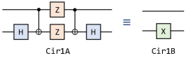
(a) Cir1

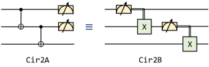
(b) Cir2

Figure 3: Two sets of equivalent circuits

Table 2: Benchmark programs

Task	Expected	No.	Programs / Pairs	#Qubits	#QuantumOps	#Programs
EQ	PASS	1	(Cir1A, Cir1B)	2	(6, 1)	4
		2	(Cir2A, Cir2B)	3	(4, 4)
		3	(QFT, QFT)	5	(17, 17)
		4	(QFT$\circ$invQFT, Empty)	5	(34, 0)
	FAIL	5	$5\times$(error Cir1A, Cir1B)	2	(6, 1)	20
		6	$2\times$(error Cir2A, Cir2B)	3	(4, 4)
		7	$3\times$(Cir2A, error Cir2B)	3	(4, 4)
		8	$5\times$(error QFT, QFT)	5	(17, 17)
		9	$5\times$(QFT$\circ$error invQFT, Empty)	5	(34, 0)
ID	PASS	10	Empty	6	0	4
		11	QFT$\circ$invQFT	5	34
		12	QPE$\circ$invQPE	5	44
		13	TeleportABA	3	60
	FAIL	14	$2\times$error Empty	6	1	17
		15	$5\times$QFT$\circ$error invQFT	5	34
		16	$5\times$QPE$\circ$error invQPE	5	44
		17	$5\times$error TeleportABA	3	60
UN	PASS	18	Cir1A	2	6	8
		19	Cir1B	2	1
		20	Empty	6	0
		21	QFT	5	17
		22	CRot	5	680
		23	$3\times$GMs of QFT	5	17
	FAIL	24	Cir2A	3	4	10
		25	Cir2B	3	4
		26	Reset	6	12
		27	$5\times$MMs of QFT	5	22
		28	$2\times$MMs of CRot	5	680

6.2 Research Questions

Our evaluation is based on the following research questions (RQs):

• RQ1: How do the parameters $k$ and $\epsilon$ affect the bug detection capability of the original algorithms?

• RQ2: Is the selection of the $s$ value, as presented in Proposition 1, effective for practical testing tasks using the original algorithms?

• RQ3: What is the performance of the optimized algorithms in terms of efficiency and bug detection accuracy?

• RQ4: How well do our checking methods perform on the benchmark programs?

6.3 Experiment Configurations

We describe our experimental configurations for each research question as follows.

$\bullet$ RQ1: We executed our algorithms on each expected-fail program, varying the values of $k$ and $\epsilon$. For EQ and UN, we examine $\epsilon$ values of 0.05, 0.10, 0.15, and 0.20. For EQ, we test $k$ values of 1, 2, 3, 4, 6, and 10. Since the UN algorithm requires two types of inputs, the minimum $k$ value we consider is 2. Thus for UN, we explore $k$ values of 2, 3, 4, 6, and 10. The corresponding $s$ values are determined as shown in Table 1. For ID, the algorithm does not involve the Swap Test, allowing for larger $k$ values. Therefore, we select $k$ values of 1, 2, 3, 4, 6, 10, 15, 20, 30, and 50. We repeat every testing process for each program 100 times and record the number of outputs returning PASS. A smaller number indicates higher effectiveness in detecting bugs. Throughout the experiment, we aim to identify a set of $k$ and $\epsilon$ values that balance between accuracy and running time.

$\bullet$ RQ2: We fix $k$ and $\epsilon$ in the EQ and UN algorithms and select different values of $s$ to run the algorithms for each expected-pass program. We calculate the value of $s_{0}$ using Proposition 1, and then choose $s=0.05s_{0}$, $0.1s_{0}$, $0.2s_{0}$, $0.3s_{0}$, $0.4s_{0}$, $0.5s_{0}$, $0.7s_{0}$, $0.9s_{0}$, and $1.0s_{0}$, respectively. We repeat the testing process for each program 100 times and record the number of outputs that return PASS. A higher number indicates fewer misjudgments by the algorithm.

$\bullet$ RQ3: We conducted experiments to evaluate the performance of the optimized algorithms - Algorithm 6 and Algorithm 7. We keep the parameters $k$, $\epsilon$, and $s$ fixed and run Algorithms 6 and 7 on both the expected-pass and expected-fail programs. The values of $k$ and $\epsilon$ are selected based on the balanced configuration determined in the experiments for RQ1, while the value of $s$ is determined using Proposition 1. We explored the impact of different values of $s$ on the algorithm’s performance. We selected $s$ values as $s$ = 1, 2, 3, 4, 6, 10, 15, 20, 30, and 50, respectively. For each benchmark program, we repeated the testing process 100 times, recording the number of outputs that returned a "PASS" result. Additionally, we kept tracking of the number of times the optimization rules were triggered during the testing. The trigger condition was defined as Algorithm 6 returning at line 6 or 11, and Algorithm 7 returning at line 5. By comparing the number of "PASS" results obtained from the optimized algorithms with those from the original algorithms and analyzing the number of triggers, we can gain insights into the performance of the optimized algorithms. This evaluation allows us to assess how effectively the optimization rules improve the algorithms’ performance.

$\bullet$ RQ4: We executed both the original and optimized algorithms for each benchmark program listed in Table 2. To ensure a balanced selection of parameters $k$, $\epsilon$, and $t$, we leveraged the findings from the experiments conducted in RQ1 and RQ3. Additionally, we calculated the value of $s$ using Proposition 1. Each program was tested 100 times, and we recorded the number of outputs that returned PASS. If an expected-pass program yielded a number close to 100 and an expected-fail program yielded a number close to 0, we can conclude that the algorithm is effective for them. Moreover, we measured the running time of both the original algorithms ($T_{0}$) and the optimized algorithms ($T_{opt}$) for each program. The ratio $T_{opt}/T_{0}$ serves as a measure of the efficiency of the optimization rules, where a smaller ratio indicates higher efficiency.

6.4 Result Analysis

6.4.1 RQ1: About parameter $k$ and $\epsilon$

The testing results for benchmark programs with different parameters $k$ and $\epsilon$ for EQ and UN are presented in Table 3, while the results with different $k$ for ID are shown in Table 4. In Table 3, "Test No. 5.1" means the 1st program/pair of No. 5 in Table 2. Similarly, the same notation is used in Table 4. Most of the results regarding the number of PASS are 0, indicating that our algorithms effectively detect failures in the expected-fail programs/pairs corresponding to the selected parameters. Notably, even a single gate or measurement mutation can lead to a significant deviation from the original program. While some programs or pairs have non-zero results, their trend suggests that the number of PASS decreases as $k$ increases and $\epsilon$ decreases. This indicates that these programs or pairs are closer to the correct version, and the selected parameters are too lenient to identify their bugs.

According to Corollary 1, the time complexity of EQ and UN is more sensitive to $\epsilon$ (which depends on $\frac{1}{\epsilon^{2}}$) than to $k$ (which depends on $k\log k$). Therefore, it is advisable to avoid choosing very small values for $\epsilon$, but $k$ can be slightly larger. Interestingly, for some programs such as No. 8.2 and No. 26.3, using excessively small $\epsilon$ does not reveal more bugs. Based on the findings in Tables 3 and 4, we proceed with $k=4$ and $\epsilon=0.15$ for EQ and UN, and $k=50$ for ID in the subsequent experiments.

Table 3: The number of PASS with different $k$ and $\epsilon$ for expected-fail programs in EQ and UN

Task		$\epsilon=0.05$						$\epsilon=0.10$						$\epsilon=0.15$						$\epsilon=0.20$
		1	2	3	4	6	10	1	2	3	4	6	10	1	2	3	4	6	10	1	2	3	4	6	10
EQ	5.1	35	10	4	2	0	0	31	10	4	1	0	0	30	9	5	2	0	0	44	18	3	2	0	0
	5.2	0	0	0	0	0	0	0	0	0	0	0	0	0	0	0	0	0	0	0	0	0	0	0	0
	5.3	16	4	0	0	0	0	12	7	1	1	0	0	18	7	1	1	0	0	28	5	1	0	0	0
	5.4	23	5	2	2	0	0	19	6	0	0	0	0	17	5	0	0	0	0	23	2	1	0	0	0
	5.5	33	12	6	0	0	0	21	14	4	2	0	0	38	15	3	1	0	0	38	9	3	1	1	0
	6.1	10	1	1	0	0	0	9	4	0	0	0	0	17	1	0	0	0	0	17	4	0	0	0	0
	6.2	58	30	25	11	4	2	53	30	17	14	4	1	81	65	46	31	16	12	78	66	54	58	36	21
	7.1	53	40	12	7	3	0	63	34	24	12	5	0	75	58	48	35	21	10	88	75	59	66	46	22
	7.2	33	11	6	0	0	0	40	12	9	1	0	0	55	34	12	6	0	1	62	47	24	23	7	1
	7.3	25	2	0	0	0	0	25	5	0	0	0	0	20	4	1	0	0	0	20	8	2	1	0	0
	8.1	0	0	0	0	0	0	0	0	0	0	0	0	0	0	0	0	0	0	0	0	0	0	0	0
	8.2	21	14	4	0	0	0	26	15	6	0	0	0	30	12	2	1	0	0	44	12	7	2	0	0
	8.3	0	0	0	0	0	0	1	0	0	0	0	0	8	1	0	0	0	0	31	10	2	0	0	0
	8.4	1	0	0	0	0	0	1	0	0	0	0	0	0	0	0	0	0	0	1	0	0	0	0	0
	8.5	2	0	0	0	0	0	1	0	0	0	0	0	1	0	0	0	0	0	3	0	0	0	0	0
	9.1	4	0	0	0	0	0	1	0	0	0	0	0	2	0	0	0	0	0	2	0	0	0	0	0
	9.2	2	0	0	0	0	0	4	0	0	0	0	0	3	0	0	0	0	0	3	0	0	0	0	0
	9.3	0	0	0	0	0	0	0	0	0	0	0	0	0	0	0	0	0	0	0	0	0	0	0	0
	9.4	0	0	0	0	0	0	0	0	0	0	0	0	0	0	0	0	0	0	0	0	0	0	0	0
	9.5	0	0	0	0	0	0	0	0	0	0	0	0	0	0	0	0	0	0	2	0	0	0	0	0
UN	24	-	0	0	0	0	0	-	0	0	0	0	0	-	0	0	0	0	0	-	0	0	0	0	0
	25	-	0	0	0	0	0	-	0	0	0	0	0	-	0	0	0	0	0	-	0	0	0	0	0
	26	-	0	0	0	0	0	-	0	0	0	0	0	-	0	0	0	0	0	-	0	0	0	0	0
	27.1	-	0	0	0	0	0	-	0	0	0	0	0	-	0	0	0	0	0	-	0	0	0	0	0
	27.2	-	0	0	0	0	0	-	0	0	0	0	0	-	0	0	0	0	0	-	0	0	0	0	0
	27.3	-	77	61	61	43	26	-	78	66	54	50	28	-	81	64	67	48	30	-	87	83	81	74	53
	27.4	-	0	0	0	0	0	-	0	0	0	0	0	-	0	0	0	0	0	-	0	0	0	0	0
	27.5	-	0	0	0	0	0	-	0	0	0	0	0	-	0	0	0	0	0	-	0	0	0	0	0
	28.1	-	6	2	1	0	0	-	6	2	1	0	0	-	5	1	0	0	0	-	8	3	2	1	0
	28.2	-	4	0	0	1	0	-	7	0	0	0	0	-	11	1	0	0	0	-	5	4	0	0	0

Table 4: The number of PASS with different $k$ for expected-fail programs in ID

Task		1	2	3	4	6	10	15	20	30	50
ID	14.1	67	46	33	22	5	0	0	0	0	0
	14.2	96	87	76	64	55	28	18	17	6	0
	15.1	26	3	0	0	0	0	0	0	0	0
	15.2	27	5	1	0	0	0	0	0	0	0
	15.3	1	0	0	0	0	0	0	0	0	0
	15.4	3	0	0	0	0	0	0	0	0	0
	15.5	28	5	1	0	0	0	0	0	0	0
	16.1	13	1	1	0	0	0	0	0	0	0
	16.2	22	7	1	0	0	0	0	0	0	0
	16.3	44	11	4	3	0	0	0	0	0	0
	16.4	49	21	8	5	0	0	0	0	0	0
	16.5	4	0	0	0	0	0	0	0	0	0
	17.1	2	0	0	0	0	0	0	0	0	0
	17.2	17	1	0	0	0	0	0	0	0	0
	17.3	18	3	1	0	0	0	0	0	0	0
	17.4	10	3	0	0	0	0	0	0	0	0
	17.5	14	0	0	0	0	0	0	0	0	0

6.4.2 RQ2: About parameter $s$

The testing results for benchmark programs with different parameters $s$ for EQ and UN are presented in Figure 4. It is evident that selecting $s=s_{0}$ leads to nearly all expected-pass programs returning PASS. This outcome demonstrates the effectiveness of the chosen parameter $s$ based on Proposition 1 in controlling type II errors. Furthermore, it is notable that the bad results (i.e., the rate of PASS is less than $1-\alpha_{2}=0.9$) is primarily observed in certain programs when $s<0.5s_{0}$. Additionally, for Test No. 1, 3, and 4, the number of PASS remains at 100 even when $s=0.05s_{0}$. This observation indicates that different programs exhibit varying degrees of sensitivity to the parameter $s$, and the selection of $s$ in Proposition 1 is conservative to ensure a high PASS rate in the worst-case scenario.

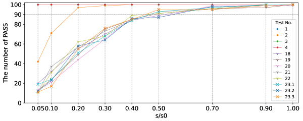
Figure 4: The number of PASS with different $s$ for expected-pass programs in EQ and UN under $k=4,\epsilon=0.15$

6.4.3 RQ3: The performance of optimized algorithms

The testing results with different $t$ for the optimized algorithms are presented in Table 5. It can be observed that most of the expected-fail programs are triggered by the optimization rules, indicating the effectiveness of our optimization rules in accelerating bug detection.

Several interesting cases, namely No. 2, No. 6.2, No. 7.1, No. 26, and No. 27.3, deserve attention. For No. 2, as $t$ increases, the number of PASS instances increases while the number of triggers decreases. It is noteworthy that Cir2A and Cir2B contain measurements (Figure 3(b)), resulting in expected mixed-state outputs. Therefore, a small value of $t$ increases the likelihood of misjudgment in this particular test scenario. In the case of No. 6.2 and No. 7.1, it appears that a small $t$ effectively excludes incorrect results. However, it is important to observe that as $t$ increases, the number of triggers decreases. This implies that returning FAIL based on optimization rules is also a misjudgment (it is similar to No. 2). No. 26 (Reset) is an intriguing case as it represents an expected-fail scenario that cannot trigger optimization rules. This is a typical example where purity preservation alone is insufficient for unitarity checking. Lastly, for No. 27.3, a significant observation is that the number of PASS instances in the optimized algorithm is considerably smaller than in the original algorithm (column ’Base’). It should be noted that the original algorithm is based on orthogonal preservation, while the optimization rule is based on purity preservation. This suggests that purity preservation checking is more effective than orthogonal preservation checking in this particular task.

Based on the results presented in Table 5, we find that $t=20$ provides a balanced choice, which we will further analyze in the subsequent overall evaluation.

6.4.4 RQ4: Overall performance for benchmark programs

The running results are shown in Table 6, including both the original algorithms and the optimized algorithms. We can see that our methods work well for most programs, i.e., the percentage of PASS is near 100 for expected-pass programs and near 0 for expected-fail programs. It means that our methods are effective for most benchmark programs with the parameters setting in the "Running Parameters" column of Table 6. The "Average Run Time" column gives the average running time in a single test.

The average running time of expected-fail programs is less than that of corresponding expected-pass programs. That is because the FAIL result is returned as long as one test point fails. Conversely, the PASS result is returned only if all test points pass. ID is faster than EQ and UN because ID does not have the repeat of the Swap Test in EQ and UN. For example, consider programs No. 4 and No. 11, which both check the relation QFT$\circ$invQFT $=I$. No. 4 uses EQ and another identity program, while No. 11 uses ID directly to check it. No. 11 requires only about one-thousandth (for the original EQ algorithm) or one-eighth (for optimized EQ algorithm) running time of No. 4. So identity checking can be implemented efficiently. It also tells us that it is valuable to find more quantum metamorphic relations, which can be reduced to identity checking.

Take note of the column labeled "$T_{opt}/T_{o}$", which indicates the efficiency of the optimization rules. We observe that for the equivalence (EQ) checking, the optimized algorithm demonstrates varying degrees of acceleration with the same parameter configuration. The acceleration ranges from dozens of percent (e.g., No. 2, No. 6.2, No. 7.1, No. 7.2, No. 7.3) to several hundred multiples (remaining EQ cases). These results indicate the effectiveness of the optimization rules for EQ. In the case of unitarity (UN) checking, the optimized algorithm is slightly slower than the original algorithm for all expected-pass cases and No.26. This is due to the additional purity preservation checking in the optimized algorithm, and they cannot be excluded by purity preservation checking. Consequently, the orthogonal checking cannot be bypassed. Nevertheless, the optimized algorithm exhibits a significant acceleration of several hundred multiples for other UN cases. Notably, the optimization may also enhance the accuracy of bug detection in some cases, such as No.27.3.

Table 6 also presents the performance of error mutation programs. However, it is observed that some error mutation programs, such as No. 6.2, No. 7.1, No. 7.2, and No. 27.3, demonstrate less effective in terms of the number of PASS outcomes. It may be because they are close to the correct one. We can solve this problem by setting the smaller $\epsilon$ and the larger $k$, as shown in Table 3. However, by Corollary  1, this implies that a super-linearly longer running time is required. Therefore, balancing the ability to find bugs and the running time is also an aspect that should be considered. In most cases, choosing too precise parameters for a few troublesome error programs may be unnecessary.

Table 5: The number of PASS and triggers by optimization rules with different $t$ for programs in EQ and UN under $k=4$, $\epsilon=0.15$ and $s$ selected by Proposition 1

			Number of PASS											Number of triggers by optimization rules
Task	Expected		Base	1	2	3	4	6	10	15	20	30	50	1	2	3	4	6	10	15	20	30	50
EQ	PASS	1	100	100	100	100	100	100	100	100	100	100	100	0	0	0	0	0	0	0	0	0	0
		2	100	4	3	8	19	38	84	94	99	100	100	96	97	92	81	62	16	6	1	0	0
		3	100	100	100	100	100	100	100	100	100	100	100	0	0	0	0	0	0	0	0	0	0
		4	100	100	100	100	100	100	100	100	100	100	100	0	0	0	0	0	0	0	0	0	0
	FAIL	5.1	2	23	4	3	1	2	0	2	3	1	1	77	96	97	99	98	100	98	97	99	99
		5.2	0	17	7	1	0	0	0	0	0	0	0	83	93	99	100	100	100	100	100	100	100
		5.3	1	23	7	1	0	0	0	0	1	0	0	77	93	99	100	100	100	100	99	100	100
		5.4	0	24	12	4	2	0	0	1	0	0	0	76	88	96	98	100	100	99	100	100	100
		5.5	1	30	12	4	2	3	1	0	1	4	2	70	88	96	98	97	99	100	99	96	98
		6.1	0	5	0	0	0	0	0	0	0	0	0	95	100	100	100	100	100	100	100	100	100
		6.2	31	3	6	3	11	14	33	42	42	42	33	93	91	83	67	48	18	3	0	0	0
		7.1	35	4	7	5	7	25	30	38	39	43	34	92	84	77	70	42	19	4	0	0	0
		7.2	6	2	2	0	2	6	7	18	8	10	12	91	87	70	66	41	14	5	0	0	0
		7.3	0	4	0	0	0	1	0	0	0	0	0	81	77	69	46	44	19	19	16	18	13
		8.1	0	2	0	0	0	0	0	0	0	0	0	98	100	100	100	100	100	100	100	100	100
		8.2	1	20	14	7	3	1	0	2	2	2	1	80	86	93	97	99	100	98	98	98	99
		8.3	0	14	0	0	0	0	0	0	0	0	0	86	99	100	100	100	100	100	100	100	100
		8.4	0	2	0	0	0	0	0	0	0	0	0	98	100	100	100	100	100	100	100	100	100
		8.5	0	0	0	0	0	0	0	0	0	0	0	100	100	100	100	100	100	100	100	100	100
		9.1	0	12	1	0	0	0	0	0	0	0	0	88	99	100	100	100	100	100	100	100	100
		9.2	0	16	2	0	0	0	0	0	0	0	0	84	98	100	100	100	100	100	100	100	100
		9.3	0	8	0	0	0	0	0	0	0	0	0	92	100	100	100	100	100	100	100	100	100
		9.4	0	6	0	0	0	0	0	0	0	0	0	94	100	100	100	100	100	100	100	100	100
		9.5	0	3	0	0	0	0	0	0	0	0	0	97	100	100	100	100	100	100	100	100	100
EQ	PASS	18	99	100	100	100	100	100	100	100	100	100	100	0	0	0	0	0	0	0	0	0	0
		19	100	100	100	100	100	100	100	100	100	100	100	0	0	0	0	0	0	0	0	0	0
		20	100	100	100	100	100	100	100	100	100	100	100	0	0	0	0	0	0	0	0	0	0
		21	99	100	100	100	100	100	100	100	100	100	100	0	0	0	0	0	0	0	0	0	0
		22	99	100	100	100	100	100	100	100	100	100	100	0	0	0	0	0	0	0	0	0	0
		23.1	99	100	100	100	100	100	100	100	100	100	100	0	0	0	0	0	0	0	0	0	0
		23.2	100	100	100	100	100	100	100	100	100	100	100	0	0	0	0	0	0	0	0	0	0
		23.3	99	100	100	100	100	100	100	100	100	100	100	0	0	0	0	0	0	0	0	0	0
	FAIL	24	0	0	0	0	0	0	0	0	0	0	0	67	93	97	98	100	100	100	100	100	100
		25	0	0	0	0	0	0	0	0	0	0	0	69	87	96	99	100	100	100	100	100	100
		26	0	0	0	0	0	0	0	0	0	0	0	0	0	0	0	0	0	0	0	0	0
		27.1	0	0	0	0	0	0	0	0	0	0	0	87	97	100	100	100	100	100	100	100	100
		27.2	0	0	0	0	0	0	0	0	0	0	0	61	76	86	83	99	97	98	98	98	100
		27.3	67	22	11	4	2	1	0	0	0	0	0	60	84	96	96	99	100	100	100	100	100
		27.4	0	0	0	0	0	0	0	0	0	0	0	91	96	100	100	100	100	100	100	100	100
		27.5	0	0	0	0	0	0	0	0	0	0	0	86	100	100	100	100	100	100	100	100	100
		28.1	0	1	0	0	0	0	0	0	0	0	0	56	79	95	98	100	100	100	100	100	100
		28.2	0	0	0	0	0	0	0	0	0	0	0	67	87	93	96	100	100	100	100	100	100

Table 6: The testing results of benchmark programs with both original algorithms and optimized algorithms

					Original Algorithm		Optimized Algorithm
Task	Running Parameters	Expected	Test No.	#Qubits	% of PASS	Average Run Time $T_{0}$	% of PASS	Average Run Time $T_{opt}$	$T_{opt}/T_{0}$
EQ	$k=4$ $s=1545$ $\epsilon=0.15$ $t=20$ for optimized algorithm.	PASS	1	2	100	3.0s	100	42ms	$1.4\times 10^{-2}$
			2	3	100	4.98s	100	4.2s	0.84
			3	5	100	21.9s	100	279ms	$1.3\times 10^{-2}$
			4	5	100	20.5s	100	283ms	$1.4\times 10^{-2}$
		FAIL	5.1	2	2	1.02s	0	15ms	$1.5\times 10^{-2}$
			5.2		0	780ms	0	9.7ms	$1.2\times 10^{-2}$
			5.3		0	1.02s	0	12ms	$1.2\times 10^{-2}$
			5.4		0	1.02s	0	13ms	$1.3\times 10^{-2}$
			5.5		0	1.2s	3	11ms	$9.2\times 10^{-3}$
			6.1	3	0	1.2s	0	9.1ms	$7.6\times 10^{-3}$
			6.2		31	3.36s	40	3.24s	0.96
			7.1	3	45	3.72s	28	2.76s	0.74
			7.2		14	2.76s	6	1.86s	0.67
			7.3		0	1.56s	0	1.32s	0.85
			8.1	5	0	5.34s	0	28ms	$5.2\times 10^{-3}$
			8.2		1	8.22s	1	70ms	$8.5\times 10^{-3}$
			8.3		0	6.18s	0	35ms	$5.7\times 10^{-3}$
			8.4		0	5.7s	0	33ms	$5.8\times 10^{-3}$
			8.5		0	5.88s	0	33ms	$5.6\times 10^{-3}$
			9.1	5	0	4.92s	0	49ms	$1.0\times 10^{-2}$
			9.2		0	5.34s	0	55ms	$1.0\times 10^{-2}$
			9.3		0	5.16s	0	52ms	$1.0\times 10^{-2}$
			9.4		0	5.22s	0	53ms	$1.0\times 10^{-2}$
			9.5		0	5.46s	0	21ms	$9.3\times 10^{-3}$
ID	$k=50$	PASS	10	6	100	12ms	N/A
			11	5	100	33ms
			12	5	100	48ms
			13	3	100	231ms
		FAIL	14.1	2	0	1.5ms
			14.2		0	2.5ms
			15.1	5	0	1.8ms
			15.2		0	1.8ms
			15.3		0	1.8ms
			15.4		0	1.8ms
			15.5		0	1.7ms
			16.1	5	0	2.2ms
			16.2		0	2.2ms
			16.3		0	2.2ms
			16.4		0	2.3ms
			16.5		0	2.2ms
			17.1	3	0	6.9ms
			17.2		0	8.2ms
			17.3		0	8.4ms
			17.4		0	7.8ms
			17.5		0	8.1ms
UN	$k=4$ $s=469$ $\epsilon=0.15$ $t=20$ for optimized algorithm.	PASS	18	2	100	421ms	100	434ms	1.03
			19	2	100	316ms	98	329ms	1.04
			20	6	100	3.3s	99	3.36s	1.02
			21	5	100	2.4s	100	2.46s	1.03
			22	5	100	5.04s	100	5.52s	1.10
			23.1	5	99	2.4s	99	2.46s	1.03
			23.2		100	2.4s	99	2.58s	1.08
			23.3		100	2.46s	99	2.52s	1.02
		FAIL	24	3	0	139ms	0	3.3ms	$2.4\times 10^{-2}$
			25	3	0	131ms	0	3.1ms	$2.4\times 10^{-2}$
			26	6	0	1.08s	0	1.14s	1.06
			27.1	5	0	583ms	0	5.3ms	$9.1\times 10^{-3}$
			27.2		0	600ms	0	32ms	$4.8\times 10^{-2}$
			27.3		74	2.6s	0	7.6ms	$1.0\times 10^{-2}$
			27.4		0	660ms	0	5.3ms	$2.9\times 10^{-3}$
			27.5		0	660ms	0	7.2ms	$1.1\times 10^{-2}$
			28.1	5	0	1.68s	0	18ms	$1.1\times 10^{-2}$
			28.2		0	1.68s	0	18ms	$1.1\times 10^{-2}$

7 Threats to Validity

Our theoretical analysis and experimental evaluation have demonstrated the effectiveness of our methods. However, like other test methods, there are still some threats to the validity of our approach.

The first challenge arises from the limitation on the number of qubits. Our equivalence and unitarity checking methods rely on the Swap Test, which requires $2n+1$ qubits for a program with $n$ qubits. Consequently, our methods can only be applied to programs that utilize less than half of the available qubits. Furthermore, when conducting testing on a classical PC simulator, the running time for large-scale programs becomes impractical.

Although we evaluated our methods on a Q# simulator, it is important to note that our algorithms may encounter difficulties when running on real quantum hardware. For instance, our methods rely on the availability of arbitrary gates, whereas some quantum hardware platforms impose restrictions on the types of quantum gates, such as only supporting the controlled gate (CNOT) on two adjacent qubits. Additionally, the presence of noise in the hardware can potentially diminish the effectiveness of our methods on real quantum hardware.

8 Related Work

We provide an overview of the related work in the field of testing quantum programs. Quantum software testing is a nascent research area still in its early stages [33, 35, 20, 52]. Various methods and techniques have been proposed for testing quantum programs from different perspectives, including quantum assertion [26, 28], search-based testing [45, 47, 48], fuzz testing [43], combinatorial testing [44], and metamorphic testing [1]. These methods aim to adapt well-established classical software testing techniques to the domain of quantum computing. Moreover, Ali et al. [2, 46] defined input-output coverage criteria for quantum program testing and employed mutation analysis to evaluate the effectiveness of these criteria. However, their coverage criteria have limitations that restrict their applicability to testing complex, multi-subroutine quantum programs. Long and Zhao [29] presented a framework for testing quantum programs with multiple subroutines. Furthermore, researchers have explored the application of mutation testing and analysis techniques to the field of quantum computing to support the testing of quantum programs [18, 17, 19, 31]. However, black-box testing for quantum programs has not been adequately addressed. In this paper, we propose novel checking algorithms for conducting equivalence, identity, and unitarity checking in black-box testing scenarios.

To the best of our knowledge, our work represents the first attempt to adapt quantum information methods to support black-box testing of quantum programs. Various methods have been proposed to address problems related to quantum systems and processes, including quantum distance estimation [16, 8], quantum discrimination [4, 50, 51], quantum tomography [42, 11], and Swap Test [7, 14]. By leveraging these methods, it is possible to conduct equivalence checking by estimating the distance between two quantum operations. Additionally, Kean et al. [9] have conducted a thorough investigation into the unitarity estimation of quantum channels. However, it should be noted that these methods are primarily tailored for quantum information processing, specifically addressing aspects such as quantum noise. Their prerequisites and methodologies are not directly applicable to the black-box testing of quantum programs.

9 Conclusion

This paper presents novel methods for checking the equivalence, identity, and unitarity of quantum programs, which play a crucial role in facilitating black-box testing of these programs. Through a combination of theoretical analysis and experimental evaluations, we have demonstrated the effectiveness of our methods. The evaluation results clearly indicate that our approaches successfully enable equivalence, identity, and unitarity checking, thereby supporting the black-box testing of quantum programs.

Several areas merit further research. First, exploring additional quantum relations and devising new checking methods for them holds promise for enhancing the scope and applicability of our approach. Second, considering quantum programs that involve both classical and quantum inputs and outputs presents an intriguing research direction, necessitating the development of appropriate modeling techniques.

Appendix

Appendix A Proof of Theorem 1

To prove Theorem 1, we need the following lemma first.

Lemma 1

Let $\mathcal{E}$ be a quantum operation on $d$-dimensional Hilbert space. Suppose it has the operator-sum representation $\mathcal{E}(\rho)=\sum_{i=1}^{d^{2}}E_{i}\rho E_{i}^{\dagger}$. $\mathcal{E}$ represents a unitary transform $U$ if and only if $\forall E_{i}$, $E_{i}=k_{i}U$, where $k_{i}$ are complex numbers satisfying $\sum_{i=1}^{d^{2}}|k_{i}|^{2}=1$.

Proof A.2.

It is obvious that $\{F_{i}\}$, where $F_{1}=U$, $F_{k}=0$ for $k>1$, is an operator-sum representation of $U$. According to Theorem 8.2 in [38], other group of elements $\{E_{i}\}$ represents $U$ if and only if $E_{i}=\sum_{j}w_{ij}F_{j}=w_{i1}U$, where all $w_{ij}$ constitutes a unitary matrix and thus $\forall j,\sum_{i}|w_{ij}|^{2}=1$. Let $k_{i}=w_{i1}$ and then $E_{i}=k_{i}U$.

Now we are able to prove Theorem 1.

Proof A.3 (for Theorem 1).

"$\Rightarrow$." Note that if $\rho$, $\sigma$ are both pure states, $tr(\rho\sigma)$ is the inner product of $\rho$ and $\sigma$. $\left|m\right>$ and $\left|n\right>$ are two different basis vectors, so $\left<m|n\right>=0$ and $\left<+_{mn}|-_{mn}\right>=0$ for $m\neq n$. A unitary transform keeps purity and inner products.

"$\Leftarrow$." Suppose $\mathcal{E}$ has the operator-sum representation $\mathcal{E}(\rho)=\sum_{i=1}E_{i}\rho E_{i}^{\dagger}$. $\mathcal{E}$ According to condition (1),

$$tr\left[\mathcal{E}(\left|m\right>\left<m\right|)\mathcal{E}(\left|n\right>\left<n\right|)\right]$$

$$=tr\left[\sum_{i,j}E_{i}\left|m\right>\left<m\right|E_{i}^{\dagger}E_{j}\left|n\right>\left<n\right|E_{j}^{\dagger}\right]$$

$$=\sum_{i,j}tr\left[E_{i}\left|m\right>\left<m\right|E_{i}^{\dagger}E_{j}\left|n\right>\left<n\right|E_{j}^{\dagger}\right]$$

$$=\sum_{i,j}\left|\left<m\right|E_{i}^{\dagger}E_{j}\left|n\right>\right|^{2}=0$$ (7)

Let $A_{ij}=E_{i}^{\dagger}E_{j}$. So $\forall i,j$ and $m\neq n$, $\left<m\right|A_{ij}\left|n\right>=0$. It means each $A_{ij}$ is diagonal on the basis $\{\left|1\right>\dots\left|d\right>\}$. According to condition (2), similarly,

$$tr\left[\mathcal{E}(\left|+_{mn}\right>\left<+_{mn}\right|)\mathcal{E}(\left|-_{mn}\right>\left<-_{mn}\right|)\right]$$

$$=\sum_{i,j}\left|\left<+_{mn}\right|A_{ij}\left|-_{mn}\right>\right|^{2}=0$$ (8)

It means $\forall i,j$,

$$\left<+_{mn}\right|A_{ij}\left|-_{mn}\right>=\frac{1}{2}(\left<m\right|+\left<n\right|)A_{ij}(\left|m\right>-\left|n\right>)=0$$ (9)

so,

$$\frac{1}{2}(\left<m\right|A_{ij}\left|m\right>-\left<m\right|A_{ij}\left|n\right>+\left<n\right|A_{ij}\left|m\right>-\left<n\right|A_{ij}\left|n\right>)$$

$$=\frac{1}{2}(\left<m\right|A_{ij}\left|m\right>-\left<n\right|A_{ij}\left|n\right>)=0$$ (10)

and thus for $m\neq n$,

$$\left<m\right|A_{ij}\left|m\right>=\left<n\right|A_{ij}\left|n\right>$$ (11)

Condition (2) selected $d-1$ combinations of $(m,n),m\neq n$ which form the edges of a connected graph with vertices $1,\dots,d$. Then from (11), we can deduce that

$$\left<1\right|A_{ij}\left|1\right>=\left<2\right|A_{ij}\left|2\right>=\dots=\left<d\right|A_{ij}\left|d\right>$$ (12)

It means the diagonal elements of $A_{ij}$ are equal, i.e., $\forall i,j,A_{ij}=E_{i}^{\dagger}E_{j}=k_{ij}I$, where $I$ is identity matrix.

For the case of $i=j$, $E_{i}^{\dagger}E_{i}=k_{ii}I$. Note that $(E_{i}^{\dagger}E_{i})^{\dagger}=E_{i}^{\dagger}E_{i}$, which means $k_{ii}$ is a non-negative real number. Let $W_{i}=\frac{1}{\sqrt{k_{ii}}}E_{i}$, then $W_{i}^{\dagger}W_{i}=I$. So $W_{i}$ is a unitary matrix and $E_{i}=\sqrt{k_{ii}}W_{i}$. From $\sum_{i}E_{i}^{\dagger}E_{i}=I$ we can deduce that $\sum_{i}k_{ii}=1$.

For the case of $i\neq j$, $E_{i}^{\dagger}E_{j}=\sqrt{k_{ii}k_{jj}}W_{i}^{\dagger}W_{j}=k_{ij}I$. Let $t_{ij}=\frac{k_{ij}}{\sqrt{k_{ii}k_{jj}}}$, then $W_{i}^{\dagger}W_{j}=t_{ij}I$ and thus $W_{j}=t_{ij}W_{i}$. Note that $W_{i}^{\dagger}W_{j}$ is a unitary matrix, so $|t_{ij}|=1$. Let $W=W_{1},t_{1}=1$, and for $j\neq 1,t_{j}=t_{1j}$, then $\forall j,W_{j}=t_{j}W$ and $E_{j}=\sqrt{k_{jj}}t_{j}W$. In addition, $\sum_{j}\left|\sqrt{k_{jj}}t_{j}\right|^{2}=\sum_{j}k_{jj}=1$. According to Lemma 1, $\mathcal{E}$ is a unitary transform.

Appendix B Proof of Proposition 1

B.1 $s$ of Equivalence Checking

Each round of the Swap Test can be seen as a Bernoulli experiment. Algorithm 2 execute three groups of Swap Test with the same number of rounds $s$. Denote the result of $i$-th round for Swap Test in lines 3, 4, and 5 as $x_{i}$, $y_{i}$, and $z_{i}$ respectively. Note that $x_{i},y_{i},z_{i}\in\{0,1\}$ and $s_{1}=\sum_{i=1}^{s}x_{i}$, $s_{2}=\sum_{i=1}^{s}y_{i}$, $s_{12}=\sum_{i=1}^{s}z_{i}$. Construct a variable $w_{i}$:

$$w_{i}=2z_{i}-x_{i}-y_{i}$$ (13)

Obviously $w_{i}\in[-2,2]$, and the mean value

$$\bar{w}=\frac{1}{s}\sum_{i=1}^{s}w_{i} =\frac{1}{s}\left(2\sum_{i=1}^{s}z_{i}-\sum_{i=1}^{s}x_{i}-\sum_{i=1}^{s}y_{i}\right)$$

$$=\frac{2s_{12}-s_{1}-s_{2}}{s}$$ (14)

In Algorithm 2, we estimate variable $r=\frac{2s_{12}-s_{1}-s_{2}}{s}=\bar{w}$. If two target programs are equivalent, whatever the input is, the distribution of every $x_{i}$, $y_{i}$, and $z_{i}$ are the same, and the expectation of $\bar{w}$:

$$E(\bar{w})=\frac{1}{s}\left(2\sum_{i=1}^{s}E(z_{i})-\sum_{i=1}^{s}E(x_{i})-\sum_{i=1}^{s}E(y_{i})\right)=0$$ (15)

According to the Hoeffding’s Inequality [25],

$$Pr(\left|\bar{w}-E(\bar{w})\right|\geq\epsilon)\leq 2e^{\frac{-2\epsilon^{2}s^{2}}{s\cdot(2-(-2))^{2}}}$$ (16)

we obtain

$$Pr(|r|\geq\epsilon)\leq 2e^{-\frac{s\epsilon^{2}}{8}}$$ (17)

$Pr(|r|\geq\epsilon)$ is the probability of failing in one test point. Note if two target programs are equivalent, it is the same for all test points. Let $P_{2}$ be the probability of passing in one test point, then

$$P_{2}>1-2e^{-\frac{s\epsilon^{2}}{8}}$$ (18)

Running testing on $k$ test points, because if one test point fails, the testing result is "FAIL," the overall probability of failing is $1-P_{2}^{k}$, and it is also the probability of type II error. To control it not to exceed $\alpha_{2}$:

$$1-P_{2}^{k}\leq\alpha_{2}$$ (19)

Then,

$$k\leq\frac{\ln(1-\alpha_{2})}{\ln P_{2}}\leq\frac{\ln(1-\alpha_{2})}{\ln(1-2e^{-\frac{s\epsilon^{2}}{8}})}$$ (20)

Figure out $s$:

$$s\geq\frac{8}{\epsilon^{2}}\ln\frac{2}{1-(1-\alpha_{2})^{\frac{1}{k}}}$$ (21)

B.2 $s$ of Unitarity Checking

In Algorithm 4, we estimate variable $r=1-\frac{2s_{1}}{s}$. If the target program $\mathcal{P}$ is unitary, for any input $(\rho,\sigma)$ selected by the algorithm, $tr(\mathcal{P}(\rho),\mathcal{P}(\sigma))=0$. So $E(r)=0$ and $E(s_{1})=\frac{s}{2}$. According to the Chernoff’s Bound [10],

$$Pr(|s_{1}-E(s_{1})|\geq\epsilon E(s_{1}))\leq 2^{-\frac{s\epsilon^{2}}{2}}$$ (22)

That is

$$Pr\left(|s_{1}-\frac{s}{2}|\geq\frac{s\epsilon}{2}\right)\leq 2^{-\frac{s\epsilon^{2}}{2}}$$

$$Pr(|r|\geq\epsilon)\leq 2^{-\frac{s\epsilon^{2}}{2}}$$ (23)

$Pr(|r|\geq\epsilon)$ is the probability of failing in one test point. Note if the target program is unitary, $Pr(|r|\geq\epsilon)$ is the same for all test points. Let $P_{2}$ be the probability of passing in one test point, then

$$P_{2}>1-2^{-\frac{s\epsilon^{2}}{2}}$$ (24)

Similarly, limit the probability of failing:

$$1-P_{2}^{k}\leq\alpha_{2}$$ (25)

Then,

$$k\leq\frac{\ln(1-\alpha_{2})}{\ln P_{2}}\leq\frac{\ln(1-\alpha_{2})}{\ln(1-2^{-\frac{s\epsilon^{2}}{2}})}$$ (26)

Figure out t:

$$s\geq\frac{2}{\epsilon^{2}}\log_{2}\frac{1}{1-(1-\alpha_{2})^{\frac{1}{k}}}$$ (27)

B.3 Proof of Formula (6)

The left less-than sign. Note that $\forall a\in(0,1)$ and $x\in\mathbb{R}$,

$$a^{x}\geq x\ln a+1$$ (28)

It deduces that

$$\frac{1}{1-a^{x}}\geq\frac{1}{-x\ln a}$$ (29)

Substitute $x$ with $1/k$ and $a$ with $1-\alpha_{2}$,

$$\frac{1}{1-(1-\alpha_{2})^{\frac{1}{k}}}\geq\frac{k}{-\ln(1-\alpha_{2})}$$ (30)

The right less-than sign. $k\geq 1$, so $1/k\in(0,1]$. Note that if $a\in(0,1)$ and $x\in[0,1]$,

$$a^{x}\leq(a-1)x+1$$ (31)

It deduces that

$$\frac{1}{1-a^{x}}\leq\frac{1}{(1-a)x}$$ (32)

Substitute $x$ with $1/k$ and $a$ with $1-\alpha_{2}$,

$$\frac{1}{1-(1-\alpha_{2})^{\frac{1}{k}}}\leq\frac{k}{\alpha_{2}}$$ (33)

References

- [1] Abreu, R., Fernandes, J. P., Llana, L., and Tavares, G. Metamorphic testing of oracle quantum programs. In 2022 IEEE/ACM 3rd International Workshop on Quantum Software Engineering (Q-SE) (2022), IEEE, pp. 16–23.
- [2] Ali, S., Arcaini, P., Wang, X., and Yue, T. Assessing the effectiveness of input and output coverage criteria for testing quantum programs. In 2021 14th IEEE Conference on Software Testing, Verification and Validation (ICST) (2021), IEEE, pp. 13–23.
- [3] Barenco, A., Berthiaume, A., Deutsch, D., Ekert, A., Jozsa, R., and Macchiavello, C. Stabilization of quantum computations by symmetrization. SIAM Journal on Computing 26, 5 (1997), 1541–1557.
- [4] Barnett, S. M., and Croke, S. Quantum state discrimination. arXiv preprint arXiv:0810.1970v1 (2008).
- [5] Beizer, B. Black-box testing: techniques for functional testing of software and systems. John Wiley & Sons, Inc., 1995.
- [6] Biamonte, J., Wittek, P., Pancotti, N., Rebentrost, P., Wiebe, N., and Lloyd, S. Quantum machine learning. Nature 549, 7671 (2017), 195–202.
- [7] Buhrman, H., Cleve, R., Watrous, J., and De Wolf, R. Quantum fingerprinting. Physical Review Letters 87, 16 (2001), 167902.
- [8] Cerezo, M., Poremba, A., Cincio, L., and Coles, P. J. Variational quantum fidelity estimation. Quantum 4 (2020), 248.
- [9] Chen, K., Wang, Q., Long, P., and Ying, M. Unitarity estimation for quantum channels. IEEE Transactions on Information Theory (2023), 1–1.
- [10] Chernoff, H. A measure of asymptotic efficiency for tests of a hypothesis based on the sum of observations. Annals of Mathematical Statistics 23, 4 (1952), 493–507.
- [11] Chuang, I. L., and Nielsen, M. A. Prescription for experimental determination of the dynamics of a quantum black box. Journal of Modern Optics 44, 11-12 (1997), 2455–2467.
- [12] D’Ariano, G. M., Paris, M. G., and Sacchi, M. F. Quantum tomography. Advances in Imaging and Electron Physics 128 (2003), 206–309.
- [13] Deutsch, D. Quantum theory, the church–turing principle and the universal quantum computer. Proceedings of the Royal Society of London. A. Mathematical and Physical Sciences 400, 1818 (1985), 97–117.
- [14] Ekert, A. K., Alves, C. M., Oi, D. K., Horodecki, M., Horodecki, P., and Kwek, L. C. Direct estimations of linear and nonlinear functionals of a quantum state. Physical review letters 88, 21 (2002), 217901.
- [15] Farhi, E., Goldstone, J., and Gutmann, S. A quantum approximate optimization algorithm. arXiv preprint arXiv:1411.4028 (2014).
- [16] Flammia, S. T., and Liu, Y.-K. Direct fidelity estimation from few pauli measurements. Phys. Rev. Lett. 106 (Jun 2011), 230501.
- [17] Fortunato, D., Campos, J., and Abreu, R. Mutation testing of quantum programs: A case study with Qiskit. IEEE Transactions on Quantum Engineering 3 (2022), 1–17.
- [18] Fortunato, D., Campos, J., and Abreu, R. Mutation testing of quantum programs written in Qiskit. In 2022 IEEE/ACM 44th International Conference on Software Engineering: Companion Proceedings (ICSE-Companion) (2022), IEEE, pp. 358–359.
- [19] Fortunato, D., Campos, J., and Abreu, R. QMutPy: a mutation testing tool for quantum algorithms and applications in Qiskit. In Proceedings of the 31st ACM SIGSOFT International Symposium on Software Testing and Analysis (2022), pp. 797–800.
- [20] García de la Barrera, A., García-Rodríguez de Guzmán, I., Polo, M., and Piattini, M. Quantum software testing: State of the art. Journal of Software: Evolution and Process (2021), e2419.
- [21] Garcia-Escartin, J. C., and Chamorro-Posada, P. Equivalent quantum circuits. arXiv preprint arXiv:1110.2998 (2011).
- [22] Grover, L. K. A fast quantum mechanical algorithm for database search. In Proceedings of the twenty-eighth annual ACM symposium on Theory of computing (1996), pp. 212–219.
- [23] Guo, J., Lou, H., Yu, J., Li, R., Fang, W., Liu, J., Long, P., Ying, S., and Ying, M. isQ: An integrated software stack for quantum programming. IEEE Transactions on Quantum Engineering (2023), 1–18.
- [24] Harrow, A. W., Hassidim, A., and Lloyd, S. Quantum algorithm for linear systems of equations. Physical review letters 103, 15 (2009), 150502.
- [25] Hoeffding, W. Probability inequalities for sums of bounded random variables. Journal of the American Statistical Association 58 (03 1963), 13–30.
- [26] Honarvar, S., Mousavi, M., and Nagarajan, R. Property-based testing of quantum programs in Q#. In First International Workshop on Quantum Software Engineering (Q-SE 2020) (2020).
- [27] Huang, Y., and Martonosi, M. Statistical assertions for validating patterns and finding bugs in quantum programs. In Proceedings of the 46th International Symposium on Computer Architecture (2019), pp. 541–553.
- [28] Li, G., Zhou, L., Yu, N., Ding, Y., Ying, M., and Xie, Y. Projection-based runtime assertions for testing and debugging quantum programs. Proceedings of the ACM on Programming Languages 4, OOPSLA (2020), 1–29.
- [29] Long, P., and Zhao, J. Testing multi-subroutine quantum programs: From unit testing to integration testing. arXiv preprint arXiv:2306.17407 (2023).
- [30] McArdle, S., Endo, S., Aspuru-Guzik, A., Benjamin, S., and Yuan, X. Quantum computational chemistry. arXiv preprint arXiv:1808.10402 (2018).
- [31] Mendiluze, E., Ali, S., Arcaini, P., and Yue, T. Muskit: A mutation analysis tool for quantum software testing. In 2021 36th IEEE/ACM International Conference on Automated Software Engineering (ASE) (2021), IEEE, pp. 1266–1270.
- [32] Mingsheng, Y. Foundations of Quantum Programming, 1st ed. Morgan Kaufmann Publishers Inc., San Francisco, CA, USA, 2016.
- [33] Miranskyy, A., and Zhang, L. On testing quantum programs. In 2019 IEEE/ACM 41st International Conference on Software Engineering: New Ideas and Emerging Results (ICSE-NIER) (2019), IEEE, pp. 57–60.
- [34] Miranskyy, A., Zhang, L., and Doliskani, J. Is your quantum program bug-free? In 2020 IEEE/ACM 42nd International Conference on Software Engineering: New Ideas and Emerging Results (ICSE-NIER) (2020), IEEE Computer Society, pp. 29–32.
- [35] Miranskyy, A., Zhang, L., and Doliskani, J. On testing and debugging quantum software. arXiv preprint arXiv:2103.09172 (2021).
- [36] Mosca, M. Cybersecurity in an era with quantum computers: Will we be ready? IEEE Security & Privacy 16, 5 (2018), 38–41.
- [37] National Academies of Sciences, E., Medicine, et al. Quantum computing: progress and prospects. National Academies Press, 2019.
- [38] Nielsen, M. A., and Chuang, I. L. Quantum Computation and Quantum Information: 10th Anniversary Edition. Cambridge University Press, 2010.
- [39] Pointing, J., Padon, O., Jia, Z., Ma, H., Hirth, A., Palsberg, J., and Aiken, A. Quanto: Optimizing quantum circuits with automatic generation of circuit identities. arXiv preprint arXiv:2111.11387 (2021).
- [40] Shor, P. W. Polynomial-time algorithms for prime factorization and discrete logarithms on a quantum computer. SIAM review 41, 2 (1999), 303–332.
- [41] Svore, K., Geller, A., Troyer, M., Azariah, J., Granade, C., Heim, B., Kliuchnikov, V., Mykhailova, M., Paz, A., and Roetteler, M. Q#: enabling scalable quantum computing and development with a high-level DSL. In Proceedings of the Real World Domain Specific Languages Workshop 2018 (2018), pp. 1–10.
- [42] Vogel, K., and Risken, H. Determination of quasiprobability distributions in terms of probability distributions for the rotated quadrature phase. Phys. Rev. A 40 (Sep 1989), 2847–2849.
- [43] Wang, J., Gao, M., Jiang, Y., Lou, J., Gao, Y., Zhang, D., and Sun, J. QuanFuzz: Fuzz testing of quantum program. arXiv preprint arXiv:1810.10310 (2018).
- [44] Wang, X., Arcaini, P., Yue, T., and Ali, S. Application of combinatorial testing to quantum programs. In 2021 IEEE 21st International Conference on Software Quality, Reliability and Security (QRS) (2021), IEEE, pp. 179–188.
- [45] Wang, X., Arcaini, P., Yue, T., and Ali, S. Generating failing test suites for quantum programs with search. In International Symposium on Search Based Software Engineering (2021), Springer, pp. 9–25.
- [46] Wang, X., Arcaini, P., Yue, T., and Ali, S. Quito: a coverage-guided test generator for quantum programs. In 2021 36th IEEE/ACM International Conference on Automated Software Engineering (ASE) (2021), IEEE, pp. 1237–1241.
- [47] Wang, X., Arcaini, P., Yue, T., and Ali, S. QuSBT: Search-based testing of quantum programs. arXiv preprint arXiv:2204.08561 (2022).
- [48] Wang, X., Yu, T., Arcaini, P., Yue, T., and Ali, S. Mutation-based test generation for quantum programs with multi-objective search. In Proceedings of the Genetic and Evolutionary Computation Conference (2022), pp. 1345–1353.
- [49] Yang, Z., Fan, J. Z., Proppe, A. H., de Arquer, F. P. G., Rossouw, D., Voznyy, O., Lan, X., Liu, M., Walters, G., Quintero-Bermudez, R., et al. Mixed-quantum-dot solar cells. Nature communications 8, 1 (2017), 1–9.
- [50] Zhang, C., Feng, Y., and Ying, M. Unambiguous discrimination of mixed quantum states. Physics Letters A 353, 4 (2006), 300–306.
- [51] Zhang, C., Wang, G., and Ying, M. Discrimination between pure states and mixed states. Phys. Rev. A 75 (Jun 2007), 062306.
- [52] Zhao, J. Quantum software engineering: Landscapes and horizons. arXiv preprint arXiv:2007.07047 (2020).
- [53] Zhao, P., Zhao, J., Miao, Z., and Lan, S. Bugs4Q: A benchmark of real bugs for quantum programs. In 2021 36th IEEE/ACM International Conference on Automated Software Engineering (ASE) (2021), IEEE, pp. 1373–1376.