HPC-driven computational reproducibility in numerical relativity codes: A use case study with IllinoisGRMHD

Abstract

Reproducibility of results is a cornerstone of the scientific method. Scientific computing encounters two challenges when aiming for this goal. Firstly, reproducibility should not depend on details of the runtime environment, such as the compiler version or computing environment, so results are verifiable by third-parties. Secondly, different versions of software code executed in the same runtime environment should produce consistent numerical results for physical quantities. In this manuscript, we test the feasibility of reproducing scientific results obtained using the IllinoisGRMHD code that is part of an open-source community software for simulation in relativistic astrophysics, the Einstein Toolkit. We verify that numerical results of simulating a single isolated neutron star with IllinoisGRMHD can be reproduced, and compare them to results reported by the code authors in 2015. We use two different supercomputers: Expanse at SDSC, and Stampede2 at TACC.

By compiling the source code archived along with the paper on both Expanse and Stampede2, we find that IllinoisGRMHD reproduces results published in its announcement paper up to errors comparable to round-off level changes in initial data parameters. We also verify that a current version of IllinoisGRMHD reproduces these results once we account for bug fixes which has occurred since the original publication.

Keywords: High-performance computing, Computational reproducibility, Numerical Relativity

1 Introduction: computational reproducibility

1.1 Defining computational reproducibility

Computational research, or scientific computing, uses advanced research computing capabilities to understand and solve complex problems in science. Computational research spans many disciplines, but at its core, it involves the development and implementation of mathematical models and numerical simulations applied to data. The main purpose of reproducibility is to verify the scientific method and outputs, and provide a mechanism to confirm or refute a study’s conclusions. That is why reproducibility is a Process, not an Achievement [1]. In this study, HPC-driven computational reproducibility has a loose definition, which is to obtain consistent scientific outputs rather than exact results using the original artifacts. This reproducibility experiment is conducted by a different team with the same experimental setup, including the same input data, the same numerical model, and following the same method and computational steps, but using a different computational environment (HPC cluster). Due to differences in compilers and hardware, some machine- and environment-specific parts of the source code, mainly configuration files need to be modified so that it can be compiled and run on a new cluster.

1.2 Computational Reproducibility and FAIR principles

The FAIR (Findable, Accessible, Interoperable, and Reusable) data principles [2], aim to enhance and support the reuse of digital material by both humans and machines. A high-level principle of computational reproducibility is to provide a clear, specific, and complete description of how a reported result was reached, although different areas of study or types of inquiry may require different kinds of information. Although scientific software differs from research data, the high-level FAIR data principles also apply to software code, in terms of the goals that ensure and improve the findability, accessibility, interoperability, reusability, transparency and optimal use of research objects. A computationally reproducible research package may include data (primary and secondary data), software program(s) and documentation (including software dependencies and runtime / computational environment) for replicating published results, and capturing related provenance information, etc. Over the last few years, a number of groups have been working towards the development of a set of FAIR guiding principles for research software (RS), including the FAIR For Research Software Working Group (FAIR4RS WG) [3, 4] which is co-led by RDA [5], FORCE11 [6], and the efforts of Research Software Alliance (ReSA) [7], the Software Sustainability Institute (SSI) [8] and grassroots communities (e.g., UK Reproducibility Network [9]).

1.3 Computational reproducibility challenges

Although research reproducibility is a critical and continuous component of the scholarly communications process, computational irreproducibility cannot be traced to one single cause. From the research software (RS) perspective, there are multiple factors that contribute to the lack of reproducibility: RS is not widely disseminated or shared and not readily discoverable and thus inaccessible, inhibiting research transparency, reproducibility and verification. As one of the steps toward scientific reproducibility, RS should be properly cited so that it is uniquely identified (e.g., the specific version of any RS package that is used to produce respective results), which also benefits transparency and traceability of research results. The Accessibility principle of the FORCE11 Software Citation Principles states that “software citations should permit and facilitate access to the software itself and to its associated metadata, documentation, data, and other materials necessary for both humans and machines to make informed use of the referenced software.” While this does not require that the RS be freely available, the metadata should be, and should provide sufficient information for the RS to be accessed and used. The development, deployment, and maintenance of reusable RS (whether computational in nature, or that relies on any software-based analysis/interpretation) are increasingly recognized internationally as a key part of facilitating trusted, reproducible research outputs and open science. Software versioning, a robust testing/quality framework (e.g. verification and validation), code repositories, and portability, all of which are recognized as desirable aspects of software quality, have all helped to drive the rapid evolution of research reproducibility. Software sustainability is key to reproducible science too, as it provides a critical tool for effective review and analysis of published results, which may lead to new research efforts. However, the wide range of robust frameworks and approaches for curating and preserving RS as a complex digital object represents a significant challenge for sustainable access, thereby hindering research reproducibility.

At the cultural and societal level, transformation to an open science-driven RS culture depends on the creation of tools, platforms and services that enable researchers to mobilize knowledge and make research processes more efficient, transparent, reproducible, and responsive to societal challenges. Specific elements of this shift include: increasing collaboration and interaction among researchers; the development of technical infrastructure that promotes the adoption of emerging research practices; the development, promotion, and adoption of open-source and open-science practices. These shifts require an agile and responsive ecosystem with strong RS workforce support and sustainable funding.

1.4 Computational reproducibility with the Einstein Toolkit

The historical lack of direct observational data in numerical relativity targeting compact objects coalescence led to simulation and the development of robust and reliable software codes being a primary scientific approach in this field. Numerical relativity (NR) is a discipline that combines general relativity with numerical simulations to study the physics of compact objects, such as binary neutron stars and black holes. NR transforms theoretical models for a system into executable codes and simulates the system using the codes to produce physical observables, such as gravitational waves, that can be detected and verified by experiments or astronomy observations, e.g. the Laser Interferometer Gravitational-Wave Observatory (LIGO). Numerical relativity codes have been crucial in the development of the gravitational wave templates used to understand the physical parameters of the binary black hole and binary neutron star systems detected by the LIGO-Virgo Collaboration [10]. With both open source and reproducibility being considered important aspects of numerical simulations, from among a selection of current open- and closed-source astrophysics codes GRChombo [11], SpECTRE [12], SpEC [13], DendroGR [14] and BAM [15] we use the Einstein Toolkit to perform our experiments due to its wide use and support of many different computing clusters.

The reproducibility experiment described here is based on a use case for the Einstein Toolkit. The Einstein Toolkit is an open-source, community-driven cyberinfrastructure ecosystem that provides key computational tools to support research in computational astrophysics, gravitational physics, and fundamental science. The Einstein Toolkit community involves experts with diverse backgrounds, from gravitational physics and astronomy to computer science and engineering. As such, the Einstein Toolkit evolves and grows—just as fundamental science itself progresses—to facilitate novel applications with ambitious science goals and high productivity of its users, and to respond to the needs of new community members.

The Einstein Toolkit is built on the Cactus [16] computational framework to connect different modules and to achieve a clean separation between science and infrastructure components. This enables domain experts in astrophysics and computer engineering to focus their efforts on the components they are most comfortable dealing with. All components within the Einstein Toolkit are distributed using free and open-source licenses enabling users to mix and match modules, adapt modules to their own needs and share these modules freely with collaborators. This arrangement, while flexible and allowing for easy collaboration among distributed and non-coordinating groups, poses both opportunities and challenges with respect to ensuring reproducible simulations.

It is worth mentioning that the numerical simulation framework — Cactus [16] already puts a premium on reproducibility and portability. In particular, the Cactus framework includes basic infrastructure to ensure the reproducibility of results as the code evolves, via its included test suite mechanism. A set of system level regression test suites consist of input descriptions for Cactus in the form of parameter files as well as expected output files and an error threshold value, which are provided by the code authors. Cactus’ infrastructure lets developers and users re-run these test suites and verify that the current code passes all test suites, and ensures all code changes that result in changes in data beyond the test suite threshold value are detected, based on which the developers can choose to either update the test data or fix the newly introduced bug.

Cactus also contains a module, “Formaline”, that collects all source files used to compile the simulation executable and embeds an archive of these files in the executable itself. In addition, Formaline generates a unique identifier for each simulation executable and each simulation run. At run time the executable outputs a copy of the included archive files along with its regular simulation output. Each output file is also tagged with the unique identifier of the simulation executable and simulation run. This way all code used to generate a set of output files are included, alongside those files and all output files record the exact code used to produce them.

Together Formaline and the test-suites provide mechanisms ensuring reproducible simulations by recording the code version used to produce results and tracking code changes that affect results.

The computational reproducibility experiment described in this paper follows the current practices of FAIR principles for data and RS, respectively. The raw simulation results and analysis code are findable and accessible through the WyoScholar data depository with doi:10.15786/20452374. The figures in this paper are reproducible with the containerized environment included in the analysis code with Docker.

2 Use case study

As a concrete example of the challenges faced in achieving computational reproducibility in HPC computations, we reproduce results obtained using the IllinoisGRMHD code [17] which was first officially included in the ET_2015_11 “Somerville” release of the Einstein Toolkit. In the manuscript announcing IllinoisGRMHD [17] the authors evolved solutions for a TOV star in general relativistic hydrodynamics and compared their results to those obtained by other codes. The TOV star is a spherically symmetric, nonrotating neutron star assuming an equation of state that represents initially cold, degenerate nuclear matter. This TOV star does not have a magnetic field. The single polytropic EOS for the TOV star is $P=K\rho^{\Gamma}$, where $K=1$, $\Gamma=2$. This is the same setup as in Appendix A of [17]. Our aim is to reproduce the results described in that paper. In the following text, we refer to IllinoisGRMHD manuscript [17] as the ILGRMHD paper, and we refer to the the ILGRMHD paper results as IGM paper results.

We perform the case study on two different supercomputers, SDSC Expanse [18] and TACC Stampede2 [19], each evolving the same dataset constituting the initial condition that was used in the ILGRMHD paper and we compared our results to IGM paper results. In order to differentiate between changes due to modifications to simulation code and changes due to differences in the supercomputer environment, we used two versions of the IllinoisGRMHD:

• the most recent IllinoisGRMHD from the ET_2022_11 “Sophie Kowalevski” release of the Einstein Toolkit, called IGM 2022 in the following

• the original IllinoisGRMHD used in [17], dubbed IGM 2015 available in [20].

IllinoisGRMHD’s complete code history is available in its public source code repository [21] using git, which we used to track down commits introducing any observed change in behavior. IGM 2015 can be found on the original publication authors’ website [22].

We choose two different supercomputers to test the consistency of Einstein Toolkit and to obtain an estimate for the sensitivity of results on the runtime environment. Consistency in our test is defined as a simulation that uses the same parameter file, and that is created using the same version of the simulation software (Einstein Toolkit ) run in different runtime environments, such as different compiler versions, hardware configurations, etc., but generating consistent numerical results for physical quantities. For example, we expect that the central density of the star oscillates with the same amplitude and frequency for simulations on Stampede2 and Expanse, but with slight differences in the numerical results due to compiler optimization, code versions and CPU model. Thus a bitwise notion of reproducibility is not useful in this context and instead a relaxed notion of reproducibility based on minimal expected changes in results due to roundoff errors is used. Roundoff error in this paper is defined the same way as in the ILGRMHD paper [17]. That is, our simulated result should agree with the claimed result at least as well as when simulating otherwise identical data perturbed by the round-off error of the underlying floating point format. More details are discussed in 2.3.1 and figure 1.

Both Expanse and Stampede2 are supported by Einstein Toolkit’s Simulation Factory [23] module, which contains information on how to compile code and submit simulations using the clusters’ resource management system. Simulation Factory is Einstein Toolkit’s primary means to maintain compatibility with computing clusters, simplifying deployment of code on supported clusters.

2.1 Experimental setup

Both IGM 2015 and IGM 2022 were compiled using Simulation Factory of IGM 2022. This is required to account for changes in the cluster environment. Both SDSC Expanse and TACC Stampede2 came online after 2015, so none of the compilation instructions of these two clusters is present in IGM 2015.

In addition, intermediate versions of IllinoisGRMHD obtained from the source code repository were compiled to pinpoint the exact commit that introduces any significant changes in output.

On all clusters the code was compiled with value-unsafe optimizations enabled implying slightly different realizations of each mathematical expression in compiled code, both between different clusters and between different compiler versions. The value-unsafe optimizations are achieved by setting various OPTIMISE flags in the machine configuration file included in the Simulation Factory. The default options for Expanse and Stampede2 configuration enabled value-unsafe optimizations, which is what we used. In addition, the the ILGRMHD paper used value-unsafe optimization in their simulations, which we are comparing with.

CPU
# of cores per node
Compiler
Optimization
MPI
# of nodes
# of MPI ranks
# of OpenMP threads

Expanse
AMD EPYC 7742
128
GCC@10.2.0
-O2 -mavx2 -mfma
openmpi/4.0.4
1
32
4

Stampede2-skx
Intel Xeon Platinum 8160
48
Intel@18.0.2
-Ofast -AVX512 -xHost
impi/18.0.2
1
24
2

Table 1: Top half: Hardware, compiler, and optimization level for each cluster. Bottom half: compute resources used in test simulation. On Expanse we used nodes in the “compute” partition, and on Stampede2, we used the nodes on “stampede2-skx” partition. Nodes on these two clusters have different hardware configurations. MPI library names, and optimization level flags are taken from Simulation Factory in IGM 2022. Differences such as these in hardware, compile and runtime environment may cause observable differences in the output of physical quantities even for identical input.

Cluster configurations and compiler versions are shown in table 1. Compiling IllinoisGRMHD on the two clusters is slightly different since compiler versions and queuing systems infrastructure differ between the two clusters. In each case, we use settings taken from Simulation Factory in IGM 2022, which supports both clusters. The key difference between the clusters, for IllinoisGRMHD, is the different CPU microarchitecture used: AMD EPYC, launched in 2017, and Intel Skylake, launched in 2015. This, combined with different compilers and aggressive optimization settings used, results in round-off level differences when evaluating mathematical expressions. These differences then propagate and, potentially, could amplify to levels incompatible with consistent physical results. On the other hand, different MPI stacks on clusters, the MPICH-based Intel MPI stack on Stampede2 and OpenMPI on Expanse, do not influence the numerical results since IllinoisGRMHD’s evolution code solely uses data transfer primitives, e.g., MPI_Send and MPI_Recv, that only copy data identically but not on reduction operations that act on values.

The code published in [17] does not include scripts to post-process the raw simulation output and plot graphs shown in the manuscript. As part of the experiment, the required scripts were implemented in Python based on information available in the published material. Additionally, copies of the original scripts were obtained from the author and are now available without modification on [20]. Their output, given identical input files, was compared to that of the newly implemented Python code.

2.2 Simulation parameters and diagnostics

Einstein Toolkit simulations are controlled via parameter files, which define numerical simulation inputs, such as grid spacing, evolution method, and initial data of the physics setup. Einstein Toolkit targets backward compatibility of parameter files – a parameter file run using Einstein Toolkit version IGM 2015 should produce numerically consistent results to that same parameter file run using any later version such as IGM 2022.

We reproduce one of the tests in the ILGRMHD paper using the original parameter file to verify this. Two simulations were created: one using IGM 2015 and the other using IGM 2022. The parameter file, tov_star_parfile_for_IllinoisGRMHD.par, used as the basis for this experiment, is included in IGM 2015 and was used with only modifications on the grid spacing corresponding to different resolutions.

All simulations use a cubic fixed mesh refinement grid, and x, y, z dimensions all have the same number of grid points. The grid spacing in high, medium, and low-resolution simulations are $(0.32,0.4,0.5)$ code units, respectively, in the coarsest refinement level. Four refinement levels of size $(1.5,3.0,6.0,12.0)\ R_{NS}$, where $R_{NS}$ is the radius of the star, are used. Therefore, the grid spacings in the finest refinement level are $\Delta x_{finest}=(0.02,0.025,0.03125)$ code units, which correspond to (75, 60, 48) grid points inside the finest refinement level.

We follow the boundary conditions as defined in [17]. For primitive variables ($\rho_{0}$, $P$, $v^{i}$), the outer boundary enforces zero-derivative, value-copy of these primitive variables to the outer boundary if the incoming velocity is positive, which is referred to as “outflow” boundary conditions in [17]. The outer boundary condition for vector potentials $A_{\mu}$ and $\sqrt{\gamma}\Phi$ is to linearly extrapolate the values to the outer boundary.

Following the conventions in [17], we use two outputs, namely, the change in central density ($\Delta\rho_{c}$) and the L2-norm of the Hamiltonian constraint violation ($\|\mathcal{H}\|$) in the numerical tests. Change in central density is defined as

$$\Delta\rho_{c}=\frac{\rho_{c}(t)-\rho_{c}(t=0)}{\rho_{c}(t=0)}\,{\rm.}$$ (1)

For a stable TOV star in equilibrium, both the change in central density and the Hamiltonian constraint violation are expected to converge to zero when resolution increases. For finite resolution both $\Delta\rho_{c}$ and $\|\mathcal{H}\|$ will have a small but nonzero value.

Convergence order is used in [17] to evaluate the performance of the code for different resolutions and as a basic check on the correct implementation of the evolution equations. For a quantity $Q\in\{\Delta\rho_{c},\|\mathcal{H}\|\}$ whose expected value is $0$, convergence order for a set of two resolutions $\Delta x_{1}$ and $\Delta x_{2}$ is computed as

$$n=\log\left(\frac{Q(\Delta x_{1})}{Q(\Delta x_{2})}\right)/\log\left(\frac{\Delta x_{1}}{\Delta x_{2}}\right)\mbox{,}$$ (2)

where $Q(\Delta x_{1,2})$ is the quantity as computed in the simulation with grid spacing $\Delta x_{1}$ and $\Delta x_{2}$, respectively.

We use two additional quantities to measure the difference in numerical results between different setups. The absolute difference in change of central density is defined as

$$\Delta^{{\rm abs}}(\Delta\rho_{c})=|\Delta\rho_{c,1}-\Delta\rho_{c,2}|$$ (3)

and the relative difference in Hamiltonian constraint violation is defined as

$$\Delta^{{\rm rel}}(\|\mathcal{H}\|)=\frac{\bigg{|}\|\mathcal{H}\|_{1}-\|\mathcal{H}\|_{2}\bigg{|}}{\|\mathcal{H}\|_{2}}\,{\rm,}$$ (4)

where relative differences are used for $\|\mathcal{H}\|$ to remove dependencies on an arbitrary overall scale for $\|\mathcal{H}\|$. In order to perform this comparison between simulations, one of the time series in the comparison may have to be interpolated to match the time steps of the other time series. Time series $1$ always has a higher sampling rate than time series $2$, and we linearly interpolate time series $1$ to match the timesteps of time series $2$. Because both time series have very high sampling rates and we downsample time series $1$ to match the other, the comparison results should not be affected by the interpolation qualitatively. Additional details are specified in the caption of each figure.

2.3 Results

After simulating the test cases included in the IGM 2015 announcement manuscript [17], we compared our simulation results with those results in [17]. In particular, the Hamiltonian constraint $\|\mathcal{H}\|$, change in central density $\Delta\rho_{c}$, and convergence order of these quantities are used to compare results across different supercomputers and to the original publication results in figure 3 of [17].

This section presents our reproducibility study results by first computing results using two different versions of the Einstein Toolkit running the same parameter file once on each of TACC Stampede2 and SDSC Expanse, respectively. Then the simulation results by the same version of the Einstein Toolkit on two different clusters are compared against each other, as well as different Einstein Toolkit versions on the same cluster.

The simulations on both clusters were run until at least $t=55\,t_{dyn}\approx 153.0$, where $t_{dyn}=\sqrt{1/\rho_{c}}$, and $\rho_{c}\approx 1.29\times 10^{-1}$ is the central density of the star at $t=0$ in $G=c=M_{\odot}=1$ unit. The numerical simulation setup and running steps of this reproducibility experiment are reproducible with details in A. Our simulation setup files, raw data, and analysis code are available at doi:10.15786/20452374.

2.3.1 Round-off level agreement between simulations

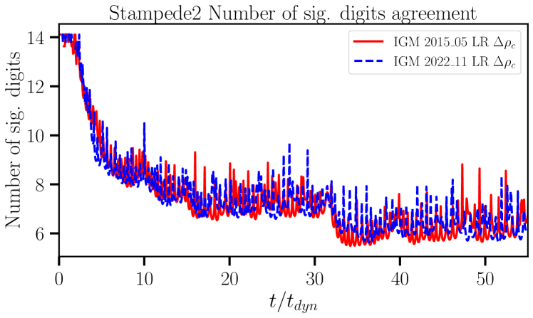
Figure 1: The number of significant digits agreement for central density changes between initial 15^th digit perturbed and unperturbed results. The red solid line is the significant digits agreement between initially perturbed results with IGM 2015 and IGM paper results. The Blue dashed line is the comparison between initially perturbed and unperturbed results with IGM 2022. Our IGM results are obtained on Stampede2.

In [17] a notion of agreement up to round-off errors is introduced by observing how two simulations, using the same executable code, whose input parameters relative difference is no more than the floating point $\epsilon$ (see C for details) deviate from each other over the course of the simulation. To understand the round-off error of our numerical experiments, we performed the same significant digits agreement test as in [17].

An initial 15^th digit random perturbation was added to the initial data on the grid in manner described in the ILGRMHD paper and repeated in appendix C. That is, at each grid point all primitive variables in IllinoisGRMHD are multiplied by a common factor $1+\epsilon$, where $\epsilon$ is a random number in the interval $[0,10^{-15})$. All conserved physical quantities are re-calculated based on the new perturbed initial primitive variables. After 30 dynamical timescales, the significant digits agreement for both IGM 2015 and IGM 2022 cases oscillate between 6 – 8 digits. Our results, as shown in figure 1, agree with the original publication result in [17] figure 1. Hence, for the set of tests considered in this manuscript, two simulations that differ by no more than an absolute error of $10^{-6}$ in $\rho$ after 30 dynamical time scales are considered to agree up to round-off level errors.

2.3.2 Expanse

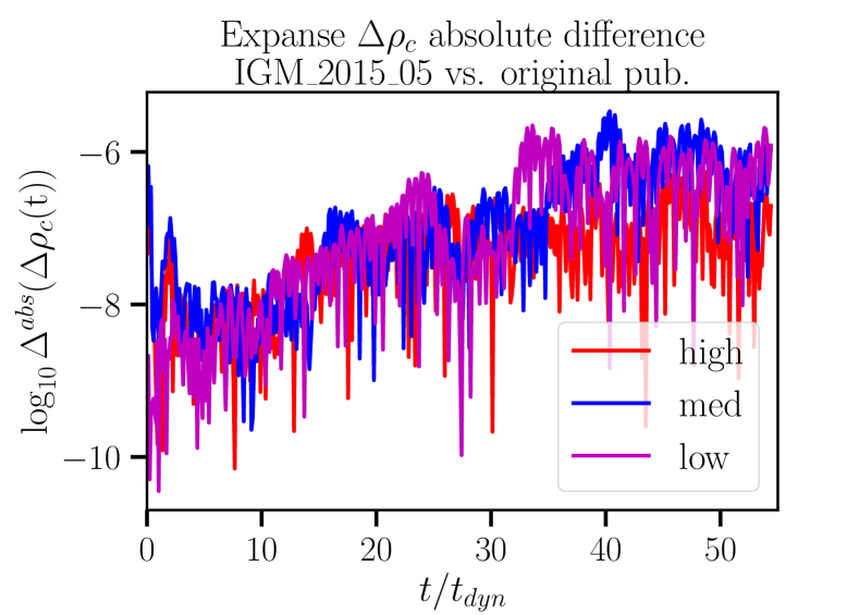
(a) IGM 2015

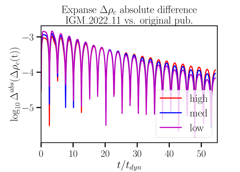
(b) IGM 2022

Figure 2: Comparing the central density changes $\Delta\rho_{c}$ for simulations created with two versions of the Einstein Toolkit on Expanse. The left two panels are for the IGM 2015, while the right two are for the IGM 2022. The upper two figures show $\Delta\rho_{c}$ and its convergence order. The bottom figures present the magnitude of the absolute error between our results and IGM paper results. The right column figures show there is a significant difference between IGM 2022 result and IGM paper results.

Figure 2 shows the agreement between our simulation result for $\Delta\rho_{c}$ and the original IGM published result. The top row shows how $\Delta\rho_{c}$ evolves when simulated using IGM 2015 and IGM 2022 and compares to the results of the ILGRMHD paper. On the left, for IGM 2015, which uses the code published in the ILGRMHD paper, our results, shown in solid, dashed, and dot-dashed lines, stop tracking the (dotted) results of the ILGRMHD paper. This is especially evident in the convergence order plot in the middle section, which shows nearly perfect agreement. This is shown explicitly in the bottom panel, which demonstrates that our results and the ILGRMHD paper differ by no more than $10^{-6}$ and are consistent within round-off error as introduced in section C.

The right-hand column displays corresponding results comparing IGM 2022 with the ILGRMHD paper. Here, differences are much more obvious, already in the top plot for $\Delta\rho_{c}$, where there is much less overlap visible between the curves. This difference is much more obvious in the convergence plot in the middle, which shows IGM 2022 having much smaller oscillations around the expected convergence of $2$. The bottom right absolute difference graph quantifies this and shows that the difference starts out very large of order $10^{-3}$ and slowly decreases to $10^{-5}$ as the simulation progresses. However, even at the end of the simulation, the difference still exceeds the threshold magnitude established for round-off level agreement. This significant difference can be tracked down to git commit 8b562af09, which is present in IGM 2022 but not in IGM 2015. We have verified that reverting this single commit brings IGM 2022 into round-off level agreement with the ILGRMHD paper. Inspecting the commit message reveals that the commit fixes a minor bug present in IGM 2015 which results in an incorrect energy density being present at $t=0$, physically corresponding to an out-of-equilibrium configuration, which explains why the observed difference decreases over time as the system relaxes back to the equilibrium configuration. We refer to this discrepancy as the incorrect initial stress-energy tensor issue.

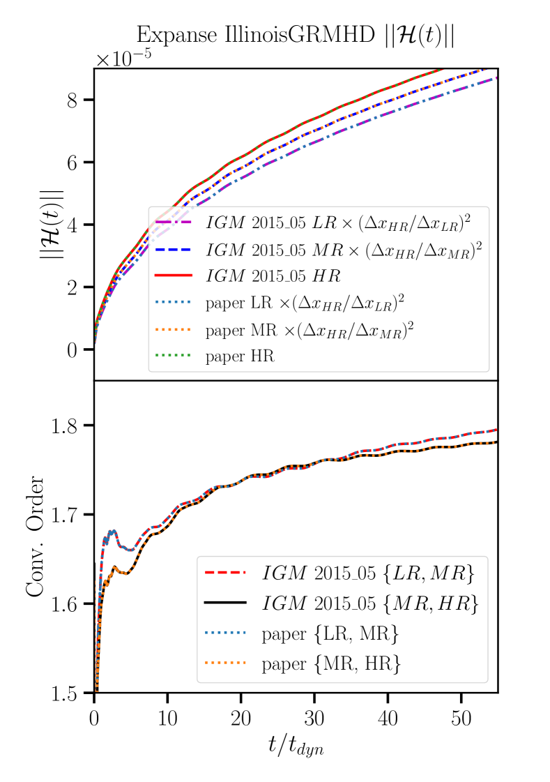
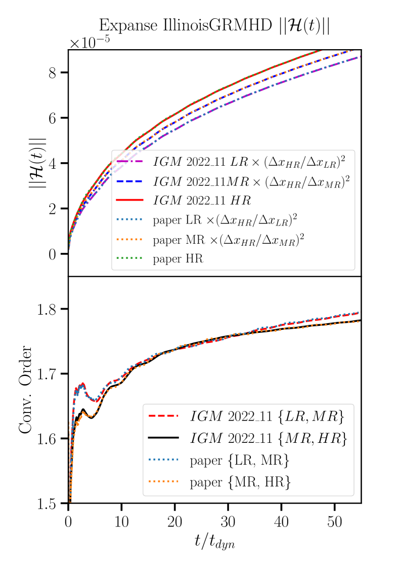
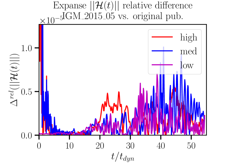
(a) IGM 2015

(b) IGM 2022

Figure 3: Comparing the Hamiltonian constraint $\|\mathcal{H}\|$ for simulations created with two versions of Einstein Toolkit on Expanse. The left panel is for the IGM 2015, and the right panel is for the IGM 2022. The upper two figures show $\|\mathcal{H}\|$ and the convergence order. The bottom two present the relative error between our results and IGM paper results.

These same observations also hold in figure 3 which displays results for the Hamiltonian constraint $\|\mathcal{H}\|$. Similar to the situation for $\Delta\rho_{c}$, our result agrees with the originally published result with IGM 2015 and has a significant difference for IGM 2022, due to the incorrect initial stress-energy tensor issue described in the previous paragraph.

2.3.3 Stampede2

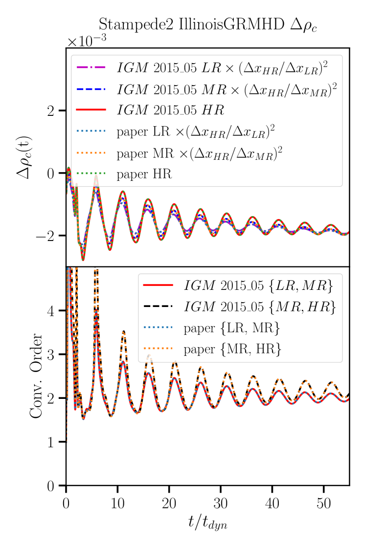
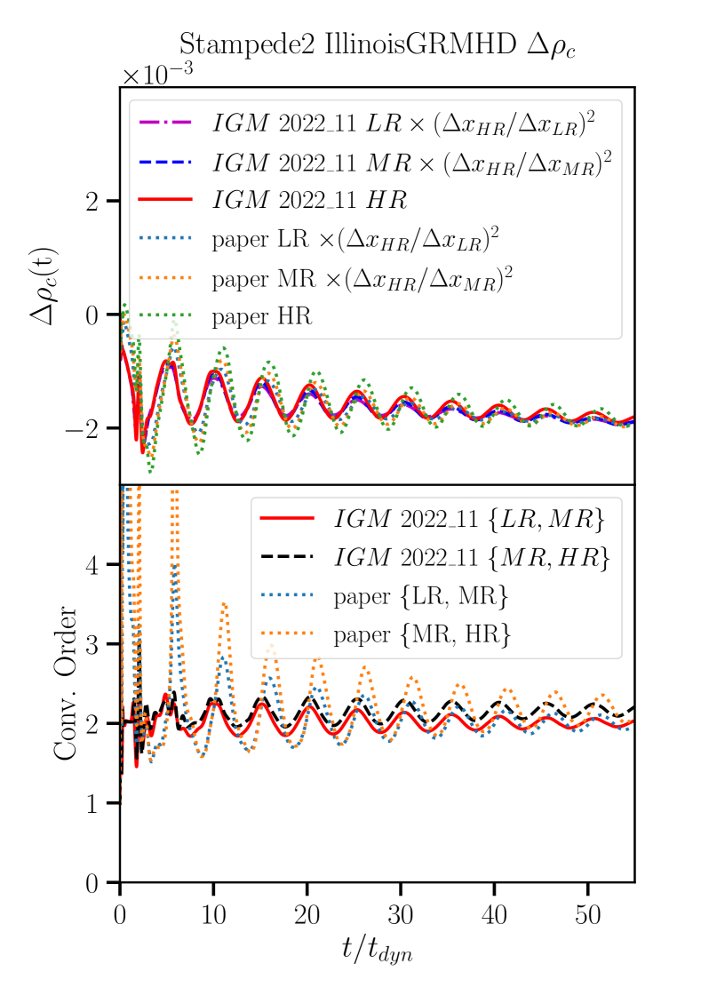
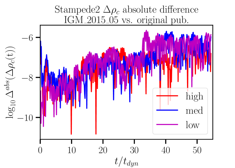
(a) IGM 2015

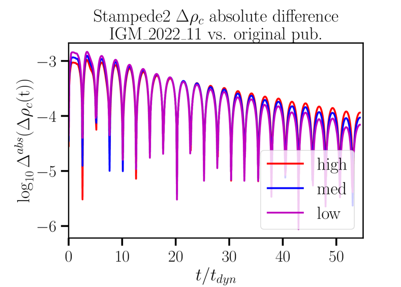
(b) IGM 2022

Figure 4: Comparing the central density changes $\Delta\rho_{c}$ for simulations created with two versions of Einstein Toolkit on Stampede2. This is the same comparison as in figure 2, but instead, the simulation was performed on Stampede2. The significant difference on the right panel is due to the incorrect stress-energy tensor issue described in section 2.3.2.

Figures 4 and 5 display equivalent results for $\Delta\rho_{c}$ and $\|\mathcal{H}\|$ obtained on Stampede2. The same effects as observed on Expanse are evident, including differences caused by changes in the source code between IGM 2015 and IGM 2022

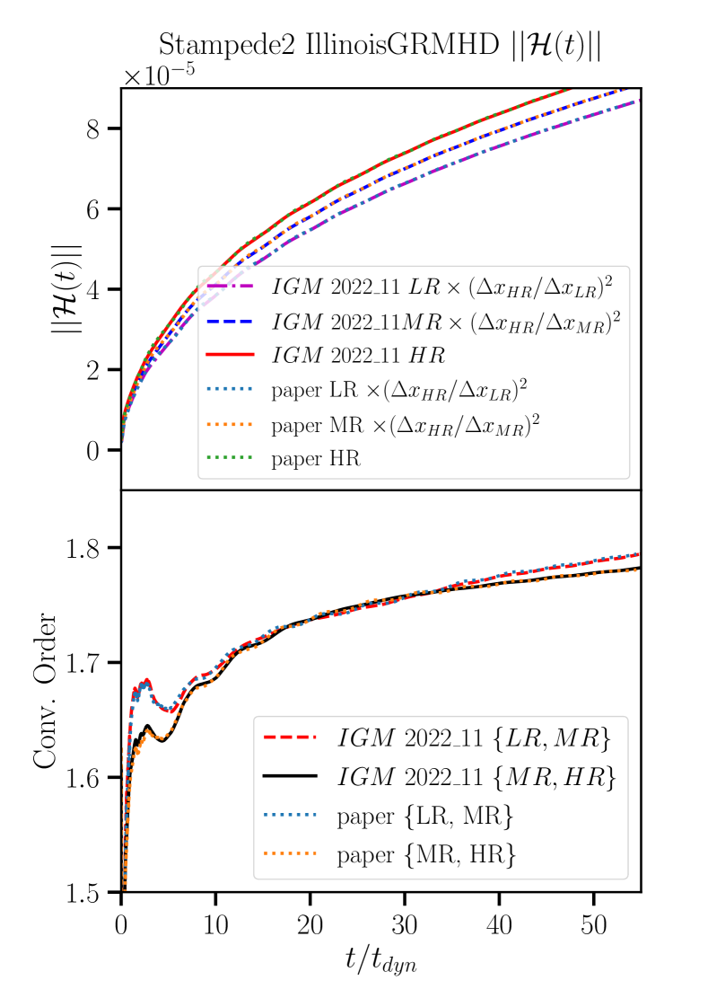
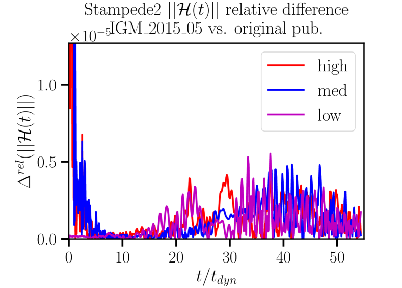
(a) IGM 2015

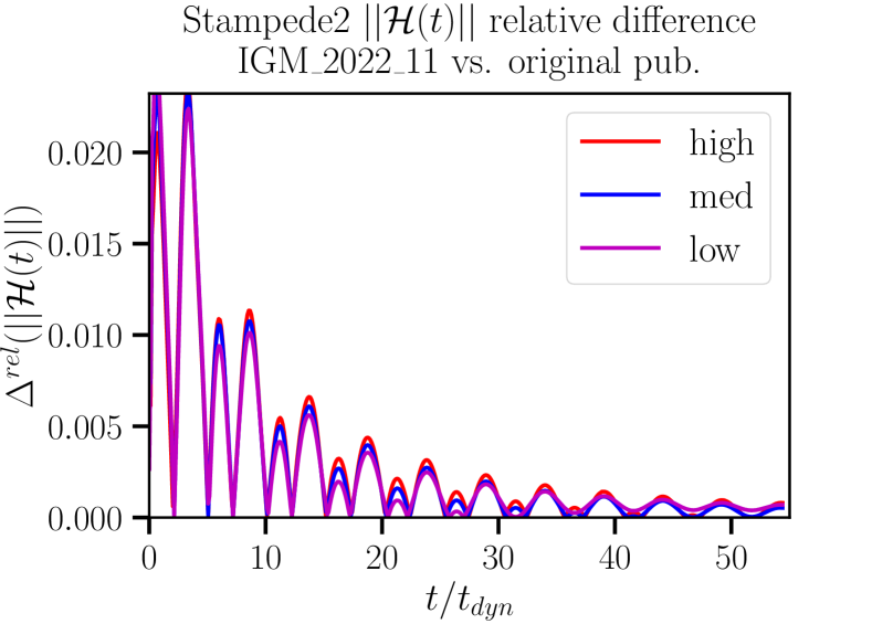
(b) IGM 2022

Figure 5: Comparing the Hamiltonian constraint $\|\mathcal{H}\|$ for simulations created with two versions of Einstein Toolkit on Stampede2. This is the same comparison as in figure 3

2.3.4 Simulation result comparison between Stampede2 and Expanse

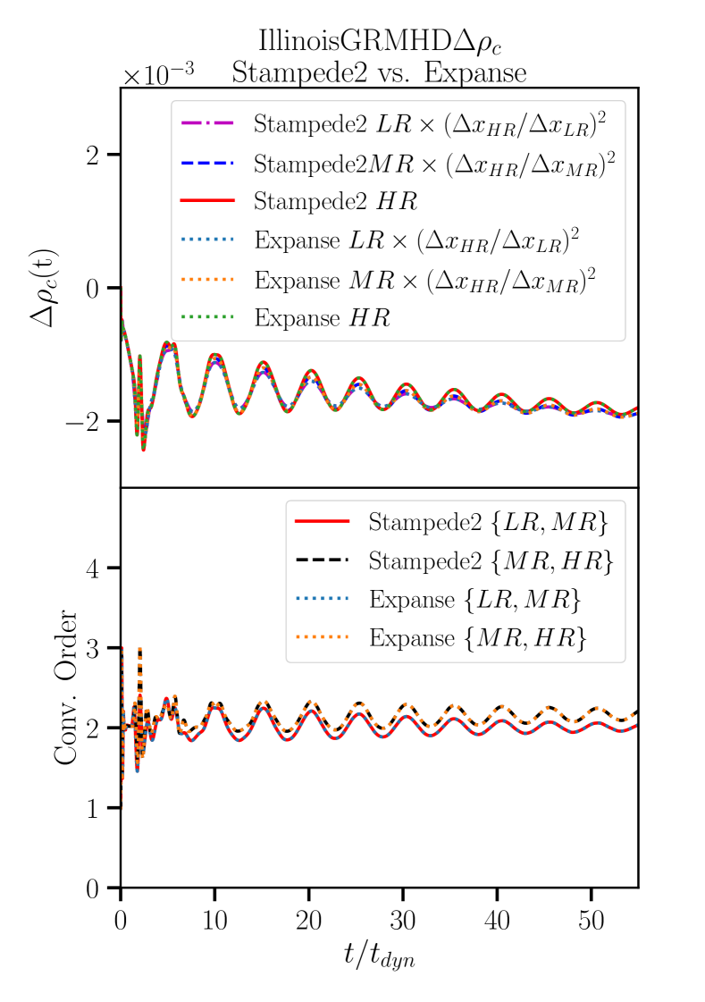
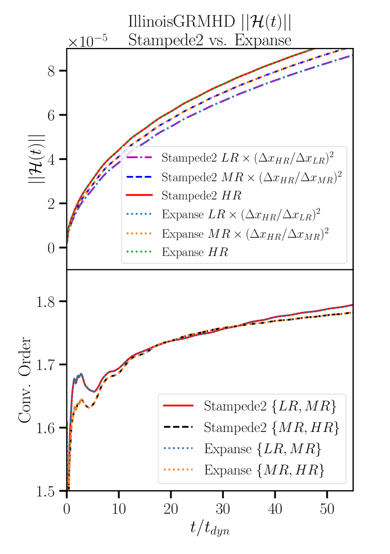
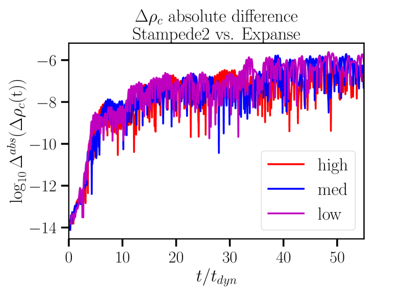
(a) $\Delta\rho_{c}$

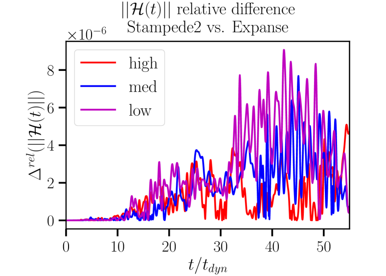
(b) $\|\mathcal{H}\|$

Figure 6: The comparison of $\Delta\rho_{c}$ and $\|\mathcal{H}\|$ on Expanse and Stampede2. Both simulations are run using IGM 2022.

Figure 6 compares results obtained using IGM 2022 on Expanse and Stampede2, respectively. For both $\Delta\rho_{c}$ and $\|\mathcal{H}\|$ results agree well within the threshold for round-off agreement. The overall results between the clusters are very similar to the results displayed in the left-hand columns of Figures 2, 3, 4, and 5 illustrating that simulations using identical source code for IGM are in round-off level agreement both when using the code in the ILGRMHD paper, and IGM 2022.

3 Conclusions

In this study, we explore two aspects of reproducibility of computational research:

1. different computing clusters using the same simulation code,

2. same computing cluster with different versions of the simulation code.

This poses challenges unique to scientific software, which is expected to compile and perform under a variety of runtime environments which are not known in advance. For example, different compute clusters employ different compilers and different compiler versions optimized for the cluster, some of which may fail to compile the scientific software without modification. In general application software, this issue is addressed by packaging all dependencies with the software, for example, in the form of container images as used by the Ubuntu SNAP format [24]. Containers are increasingly available on HPC systems [25, 26] providing a way to encapsulate all code dependencies except the operating system kernel with the science code. This, however, typically entails a loss of efficiency that may be unacceptable for high-performance computing [27, 28], and compiling from source remains the norm for HPC codes in the current state of scientific software.

With this caveat, we observed that the same simulation code produced results agreeing to the round-off level. Our simulations using IGM 2015 agree with the original publication results on both Hamiltonian constraint and central density drift to round-off level, as shown in the lower left panel of figures 2, 3, 4, and 5.

During our experimentation with IGM 2015, we identified two minor discrepancies in the ILGRMHD paper. The first discrepancy concerns the description of the perturbation used in Section 4.1; it is accurately described in Section 4.2 of the ILGRMHD paper but incorrectly presented in Section 4.1. Specifically, the factor $\epsilon$ of the perturbation $1+\epsilon$ is a random number generated within the range $[0,10^{-15})$, contrary to the fixed number $10^{-15}$ stated in Section 4.1 of the ILGRMHD paper. Second, our simulations using IGM 2022 showed discrepancies from the IGM paper results as we stated in section 2.3.2. We tracked down to a change in the source code, and reverting this change restored the reproducibility of IGM paper results.

Computational reproducibility is essential to the continuing development of scientific software, especially when a new module or functionality is added. In addition, it is also critical for the use of scientific code by others and the verification of results by others.

Furthermore, long-term computational reproducibility is an important aspect researchers be aware of. New researchers joining the field should be able to track and understand how to reproduce and interpret existing numerical experiment results. With this in mind, we suggest best practices for manuscripts announcing new scientific software or simulation results.

• Creating a DOI for specific versions of source code or depositing the source code used in the paper. To help the scientific community reproduce the results, it is recommended that papers include a trackable identifier such as DOI or Git Hash. With these unique identifiers, the simulation results and the software itself can be understood.

• Attaching parameter files as supplemental materials to the paper. If the parameter files cannot be submitted as supplemental material, authors should create a DOI for parameter files used to run simulations that produce results claimed in the paper. Due to newer versions of the Einstein Toolkit, we found that we have to change some parameters of the simulation parameter files to reproduce the results claimed in the ILGRMHD paper. Along with a trackable version of the simulation software, a parameter file associated with a DOI makes the simulation easy to reproduce, and the simulation workflow transparent.

• Separate the computational and physical discussion. Authors for a paper with numerical experiment results should have separate sections to discuss the physical result and computational results, and how to reproduce them. Theories and problem setups should be discussed in the physical result part. Numerical experiment setups, such as simulation framework and parameter files should be introduced in the computational result section.

In conclusion, this work studied the challenges encountered when reproducing scientific results obtained with a state-of-the-art, real-world science code when applied to a common test problem. This test problem was originally used to verify both code correctness and performance in the ILGRMHD paper.

Science codes, and compilers used in high-performance computing architectures, are not designed to provide bit-identical results despite identical source code and input, instead allowing for deviations to some extent between results as long as those deviations are considered “small” compared to intrinsic approximation and discretization errors of the method used.

Additionally, scientific codes are undergoing constant changes as bugs are discovered and fixed and new features are added to them to study new phenomena. These changes result in numeric values differing at levels above round-off error deviations. Often these fixes are only documented in a revision control system and not in an explicit change log file. A key task of determining reproducibility is thus to identify these value changing bug-fixes and quantify whether the observed differences are compatible with the change introduced to the code. Hitherto, this process requires an expert understanding of the science code and is not automated.

We demonstrate that, within these constraints, results obtained using IGM 2015 can be independently reproduced on multiple clusters and with multiple versions of IllinoisGRMHD. We also provide suggestions to remedy some computational challenges encountered in this reproducibility study.

4 Future work

In this work, we have not attempted to extend the notion of reproducibility past value changing bug fixes in the code. Some codes, for example [29], attempt to address this issue by explicitly marking commits that introduce single-bit changes in results while others [30] record a level of fuzziness within which results are considered equal. Neither approach seems fully satisfactory and a more robust method based on the notion of equal up to round-off error may help provide a better handle on code changes that affect reproducing scientific results.

Data availability statement

The data that support the findings of this study are openly available in the WyoScholar data repository at doi:10.15786/20452374.

Code availability statement

The simulation codes used in this study are openly available. IGM 2015 is available at doi:10.5281/zenodo.7545717. IGM 2022, which is part of Einstein Toolkit ET_2022_11 “Sophie Kowalevski” release, is available at doi:10.5281/zenodo.7245853. The data analysis and visualization codes used to generate figures in this manuscript are publicly available at doi:10.15786/20452374.

Appendix A Steps to compile the codes

In the following section, we provide detailed instructions on how to compile the codes, IGM 2015 and IGM 2022, on the two clusters, Expanse and Stampede2. IGM 2015 is the code used in the ILGRMHD paper available from its author’s website and from [20]. IGM 2022 is the “Sophie Kowalevski” (ET_2022_11) release of the Einstein Toolkit available from [31]. To compile IGM 2022 on either Expanse or Stampede2-skx, the steps are documented on the Einstein Toolkit website [31]

Listing 1: Compiling IGM 2022

⬇

curl -kLO \

https://raw.githubusercontent.com/gridaphobe/CRL/ET_2022_11/GetComponents

chmod a+x GetComponents

./GetComponents --parallel \

https://bitbucket.org/einsteintoolkit/manifest/raw/ET_2022_11/\

einsteintoolkit.th

cd Cactus

./simfactory/bin/sim setup-silent

./simfactory/bin/sim build --thornlist thornlists/einsteintoolkit.th

is sufficient. Compiling IGM 2015 on the other hand, due to changes in compilers and cluster environment, requires some additional steps.

We begin by downloading the code from [20]:

Listing 2: IGM 2015: step 1

⬇

curl -OL ’https://zenodo.org/record/7545717/files/IllinoisGRMHD_’\

’Sept_1_2015_public_release__based_on_ET_2015_05.tar.gz’

tar xf IllinoisGRMHD_Sept_1_2015_public_release__based_on_ET_2015_05.tar.gz

cd IllinoisGRMHD_Sept_1_2015_public_release__based_on_ET_2015_05

Next we replace Simfactory2015 with Simfactory2022 to use its machine definition files

Listing 3: IGM 2015: step 2

⬇

rm -r simfactory

cp -a ../Cactus/simfactory/ simfactory

Step 3: IGM 2015 contains legacy code that GCC version 10 and newer flags as invalid and requires adding -fallow-argument-mismatch to F90FLAGS and F77FLAGS variables, and -fcommon to CFLAGS and CXXFLAGS variables in simfactory/mdb/optionlists/expanse-gnu.cfg. Step 4: Simfactory2022 no longer provides F77, F77FLAGS, F77_DEBUG_FLAGS, F77_OPTIMISE_FLAGS, F77_NO_OPTIMISE_FLAGS, F77_PROFILE_FLAGS, F77_OPENMP_FLAGS, and F77_WARN_FLAGS and instead uses F90 etc. throughout. To compile IGM 2015 we duplicate all F90 settings and rename the copies to F77 settings in simfactory/mdb/optionlists/stampede2-skx.cfg. Intel compilers version 17 or higher contain an apparent compiler bug at high optimization levels that makes them fail to compile file bbox.cc. Thus we add

Listing 4: IGM 2015: step 5

⬇

#if __INTEL_COMPILER >= 1700

#pragma GCC optimization_level 1

#endif

at the top of repos/carpet/CarpetLib/src/bbox.cc. With these modifications in place we compile using the ThornList file supplied in the main directory of IGM 2015:

Listing 5: IGM 2015: step 6

⬇

cd IllinoisGRMHD_Sept_1_2015_public_release__based_on_ET_2015_05

./simfactory/bin/sim setup-silent

./simfactory/bin/sim build --thornlist ThornList

Appendix B Steps to start the simulations

We use a modified version of the file exe/tov_star_parfile_for_IllinoisGRMHD.par included in IGM 2015. The included parameter file is set up for a short validity test and requires some modification to match the file used in [17]. Step 1: we change the value of CoordBase::dx, CoordBase::dy, and CoordBase::dz from $1.0$ to $0.5$, $0.4$, and $0.32$ for low-resolution, medium-resolution, and high-resolution simulations, respectively.
Step 2: we enable the time termination condition and set the final time to $155$

Listing 6: Final time

⬇

#cactus::cctk_itlast = 128

Cactus::terminate = "time"

Cactus::cctk_final_time = 155

Step 3: for convenience of output we change IO::out_dir’s value to $parfile.
Step 4: finally we add checkpointing and recovery options at the end of the file:

Listing 7: Termination and checkpoint

⬇

ActiveThorns = TerminationTrigger

TerminationTrigger::max_walltime = @WALLTIME_HOURS@

# Trigger termination 30 minutes before the walltime is reached

TerminationTrigger::on_remaining_walltime = 30

TerminationTrigger::output_remtime_every_minutes = 30

TerminationTrigger::termination_from_file = yes

TerminationTrigger::termination_file = "terminate.txt"

TerminationTrigger::create_termination_file = yes

CarpetIOHDF5::checkpoint = yes

IO::recover = "autoprobe"

IO::checkpoint_on_terminate = yes

Appendix C Steps to compute expected round-off level differences

We estimate the effect of round-off level changes induced, e.g., by compiler applied code optimization on the time evolution of results by explicitly adding a small, random perturbation of $10^{-15}$ relative size to the initial data for all primitive variables. Comparing the results of this perturbed initial data with an unperturbed simulation provides an estimate for these effects and establishes an order of magnitude estimate for which differences are compatible with round-off level changes in the data.

IGM 2022 already contains facilities to add such a perturbation in the ID_converter_ILGRMHD module:

Listing 8: Random perturbation

⬇

ID_converter_ILGRMHD::random_pert = 1e-15

IGM 2015 on the other hand contains a bug that renders the parameter ineffectual and we apply the git commit hash f822e2278695615a9ad508d58fe25b0c94451a31 “WVUThorns/ID_converter_ILGRMHD: When adding an optional perturbation to the initial data, the perturbation should be applied to all IllinoisGRMHD quantities, not HydroBase, at this part of the routine. Behavior was correct except for density. This one-line patch fixes that.” from IGM 2022 which fixes the bug.

References

References

- [1] Lin J and Zhang Q 2020 Reproducibility is a process, not an achievement: The replicability of IR reproducibility experiments Advances in Information Retrieval ed Jose J M, Yilmaz E, Magalhães J, Castells P, Ferro N, Silva M J and Martins F (Cham: Springer International Publishing) pp 43–49 ISBN 978-3-030-45442-5
- [2] Wilkinson M D, Dumontier M, Aalbersberg I J, Appleton G, Axton M, Baak A, Blomberg N, Boiten J W, da Silva Santos L B, Bourne P E et al. 2016 Scientific data 3 1–9
- [3] 2022 FAIR for research software (FAIR4RS) WG URL https://www.rd-alliance.org/groups/fair-4-research-software-fair4rs-wg
- [4] Martinez P A 2020 Towards FAIR principles for research software URL https://eresearchnz.figshare.com/articles/presentation/Towards_FAIR_principles_for_research_software/11929617/1
- [5] RDA | research data sharing without barriers https://www.rd-alliance.org/ URL https://www.rd-alliance.org/
- [6] FORCE11 the future of research communications and e-scholarship https://force11.org/ URL https://force11.org/
- [7] 2022 <ReSA> research software alliance URL https://www.researchsoft.org/
- [8] 2022 The software sustainability institute URL https://software.ac.uk/
- [9] UK reproducibility network https://www.ukrn.org/ URL https://www.ukrn.org/
- [10] Abbott B P e a (LIGO Scientific Collaboration and Virgo Collaboration) 2016 Phys. Rev. Lett. 116(6) 061102 URL https://link.aps.org/doi/10.1103/PhysRevLett.116.061102
- [11] Andrade T, Salo L A, Aurrekoetxea J C, Bamber J, Clough K, Croft R, de Jong E, Drew A, Duran A, Ferreira P G, Figueras P, Finkel H, França T, Ge B X, Gu C, Helfer T, Jäykkä J, Joana C, Kunesch M, Kornet K, Lim E A, Muia F, Nazari Z, Radia M, Ripley J, Shellard P, Sperhake U, Traykova D, Tunyasuvunakool S, Wang Z, Widdicombe J Y and Wong K 2021 Journal of Open Source Software 6 3703 URL https://doi.org/10.21105/joss.03703
- [12] Deppe N, Throwe W, Kidder L E, Vu N L, Hébert F, Moxon J, Armaza C, Bonilla G S, Kim Y, Kumar P, Lovelace G, Macedo A, Nelli K C, O’Shea E, Pfeiffer H P, Scheel M A, Teukolsky S A, Wittek N A et al. 2023 SpECTRE v2023.02.09 10.5281/zenodo.7626579 URL https://spectre-code.org
- [13] Spec: Spectral einstein code URL https://www.black-holes.org/code/SpEC.html
- [14] Fernando M, Neilsen D, Lim H, Hirschmann E and Sundar H 2019 SIAM Journal on Scientific Computing 41 C97–C138 (Preprint https://doi.org/10.1137/18M1196972) URL https://doi.org/10.1137/18M1196972
- [15] Bruegmann B, Tichy W and Jansen N 2004 Phys. Rev. Lett. 92 211101 (Preprint gr-qc/0312112)
- [16] Cactus Computational Toolkit URL http://www.cactuscode.org/
- [17] Etienne Z B, Paschalidis V, Haas R, Mösta P and Shapiro S L 2015 Class. Quant. Grav. 32 175009 (Preprint arXiv:1501.07276[astro-ph.HE])
- [18] SDSC https://www.sdsc.edu/support/user_guides/expanse.html URL https://www.sdsc.edu/support/user_guides/expanse.html
- [19] TACC https://portal.tacc.utexas.edu/user-guides/stampede2#table1 URL https://portal.tacc.utexas.edu/user-guides/stampede2#table1
- [20] Etienne Z 2022 IllinoisGRMHD2015 simulation software package and raw dataset URL https://doi.org/10.5281/zenodo.7545717
- [21] Etienne Z https://bitbucket.org/zach_etienne/wvuthorns.git URL https://bitbucket.org/zach_etienne/wvuthorns.git
- [22] Etienne Z http://astro.phys.wvu.edu/zetienne/ILGRMHD/ URL http://astro.phys.wvu.edu/zetienne/ILGRMHD/
- [23] SimFactory: Herding numerical simulations URL http://simfactory.org/
- [24] About Snaps https://snapcraft.io/about URL https://snapcraft.io/about
- [25] Jacobsen D M and Canon R S 2015
- [26] Kurtzer G M, Sochat V and Bauer M W 2017 PLOS ONE 12 1–20 URL https://doi.org/10.1371/journal.pone.0177459
- [27] Ben-Nun T, Gamblin T, Hollman D S, Krishnan H and Newburn C J 2020 Workflows are the new applications: Challenges in performance, portability, and productivity 2020 IEEE/ACM International Workshop on Performance, Portability and Productivity in HPC (P3HPC) pp 57–69
- [28] Canon R S and Younge A 2019 A case for portability and reproducibility of HPC containers 2019 IEEE/ACM International Workshop on Containers and New Orchestration Paradigms for Isolated Environments in HPC (CANOPIE-HPC) pp 49–54
- [29] 2021 SpEC: Spectral Einstein Code URL https://www.black-holes.org/code/SpEC.html
- [30] Etienne Z, Brandt S R, Diener P, Gabella W E, Gracia-Linares M, Haas R, Kedia A, Alcubierre M, Alic D, Allen G, Ansorg M, Babiuc-Hamilton M, Baiotti L, Benger W, Bentivegna E, Bernuzzi S, Bode T, Bozzola G, Brendal B, Bruegmann B, Campanelli M, Cipolletta F, Corvino G, Cupp S, Pietri R D, Dimmelmeier H, Dooley R, Dorband N, Elley M, Khamra Y E, Faber J, Font T, Frieben J, Giacomazzo B, Goodale T, Gundlach C, Hawke I, Hawley S, Hinder I, Huerta E A, Husa S, Iyer S, Johnson D, Kellermann T, Knapp A, Koppitz M, Laguna P, Lanferman G, Löffler F, Masso J, Menger L, Merzky A, Miller J M, Miller M, Moesta P, Montero P, Mundim B, Nerozzi A, Noble S C, Ott C, Paruchuri R, Pollney D, Radice D, Radke T, Reisswig C, Rezzolla L, Rideout D, Ripeanu M, Sala L, Schewtschenko J A, Schnetter E, Schutz B, Seidel E, Seidel E, Shalf J, Sible K, Sperhake U, Stergioulas N, Suen W M, Szilagyi B, Takahashi R, Thomas M, Thornburg J, Tobias M, Tonita A, Walker P, Wan M B, Wardell B, Werneck L, Witek H, Zilhão M, Zink B and Zlochower Y 2021 The Einstein Toolkit to find out more, visit http://einsteintoolkit.org URL https://doi.org/10.5281/zenodo.4884780
- [31] Einstein Toolkit: Open software for relativistic astrophysics URL http://einsteintoolkit.org/