The performance of approximate equation of motion coupled cluster for valence and core states of heavy element systems

Abstract

The equation of motion coupled cluster singles and doubles model (EOM-CCSD) is an accurate, black-box correlated electronic structure approach to investigate electronically excited states and electron attachment or detachment processes. It has also served as a basis for developing less computationally expensive approximate models such as partitioned EOM-CCSD (P-EOM-CCSD), the second-order many-body perturbation theory EOM (EOM-MBPT(2)), and their combination (P-EOM-MBPT(2)) [S. Gwaltney et al., Chem. Phys. Lett. 248, 189-198 (1996)]. In this work we outline an implementation of these approximations for four-component based Hamiltonians and investigate their accuracy relative to EOM-CCSD for valence excitations, valence and core ionizations and electron attachment, and this for a number of systems of atmospheric or astrophysical interest containing elements across the periodic table. We have found that across the different systems and electronic states of different nature considered, partition EOM-CCSD yields results with the largest deviations from the reference, whereas second-order based approaches tend show a generally better agreement with EOM-CCSD. We trace this behavior to the imbalance brought about by the removal of excited state relaxation in the partition approaches, with respect to degree of electron correlation recovered.

I Introduction

Developments in electronic structure methods of recent decades Loos, Scemama, and Jacquemin (2020); Bokarev and Kühn (2019); Izsák (2019) have allowed theory to play a more important role in helping interpret increasingly complex experiments. One case arises in connection to the recent developments on coherent light sources such as those generated in synchrotrons Alov (2005); Fadley (2010); Doucet and Baruchel (2016); Couprie (2014) or X-ray free-electron lasers (XFEL) Bergmann, Yachandra, and Yano (2017); Young et al. (2018), which have enabled significant improvements in resolution when exploring high-energy processes involving electronic excitations, such as in X-ray absorption spectroscopy (XAS). But theory can also be of help in lower-energy regimes, be in photoionization experiments Gunzer, Krüger, and Grotemeyer (2018) in UV/visible energy range or in the determination of electron affinities Rienstra-Kiracofe et al. (2002); Richard et al. (2016); Chakraborty and Nandi (2020).

Among the approaches that are generally capable of treating core and valence excited states, as well as states representing electron attachment and detachment processes, we find methods such as complete-active space second-order perturbation theory (CASPT2) Grell et al. (2015); Lundberg and Delcey (2019) and multireference CI (MRCI) Maganas et al. (2019), which thanks to their flexibility can describe systems which are multiconfigurational already for their ground states. Multi-reference coupled cluster approaches such as the state-specific (SS-MRCC) approach of Brabec et al. (2012), the state-universal (UGA-SUMRCC) approach of Sen, Shee, and Mukherjee (2013) and the valence-universal (IH-FSCC) approach of Dutta et al. (2014a) have also been successfully applied to investigate core spectra, though their use has been more limited than that of MRCI or CASPT2. And more recently, a mulireference extension of the algebraic diagrammatic construction (ADC) family of methods Dreuw and Wormit (2014); Wenzel, Wormit, and Dreuw (2014) by Mazin and Sokolov (2023) has been proposed to address core spectra.

For systems which the ground-state can be well-represented by a single configuration an array of other methods are also available, such as time-dependent DFT (TD-DFT) Besley (2020, 2021); Brena and Luo (2006); Fouda and Besley (2017); Santis, Vallet, and Gomes (2022), the ADC family of methods Dreuw and Wormit (2014); Wenzel, Wormit, and Dreuw (2014), as well as the family of methods based on coupled cluster theory, such as linear-response (LR-CC) Koch et al. (1990); Coriani and Koch (2015) and equation of motion (EOM) Bartlett and Musiał (2007); Coriani et al. (2012); Coriani and Koch (2015); Sadybekov and Krylov (2017); Vidal et al. (2019); Peng et al. (2015); Park, Perera, and Bartlett (2019); Matthews (2020) coupled cluster. EOM-CC is closely connected to the valence-universal multireference Fock-space coupled cluster (FSCC) approach (see Musial and Bartlett (2008a) for a detailed analysis of the two formalisms) and will yield results which are indistingushable from FSCC for ionization energies Shee et al. (2018) (if the FSCC model spaces are flexible enough), though for excited states it tends to overestimate the FSCC energies Musial and Bartlett (2008b, a); Réal et al. (2009).

It should be noted that for certain situations such as in the calculation of core and valence ionization energies, methods based on the calculation of energy differences (such $\Delta$HF Bagus (1965); Bagus et al. (1999); Naves de Brito et al. (1991), $\Delta$MP2 Shim et al. (2011); South et al. (2016), $\Delta$DFT Besley, Gilbert, and Gill (2009); Fouda and Besley (2017); Pueyo Bellafont, Bagus, and Illas (2015); Takahata and Chong (2012), $\Delta$CC Watts and Bartlett (1990); Zheng and Cheng (2019)) can be very useful, since they are very effective in accounting for orbital relaxation (upon ionization) and electron correlation, but at the expense of requiring the solution of the mean-field problem for open-shells that may be difficult to converge, not to mention the need to find broken symmetry solutions when equivalent centers are present.

Thus, when single-reference approaches are applicable, a good balance between ease of use and accuracy for both valence and core processes is found in coupled cluster based approaches such as EOM-CC (or equivalently LR-CC) based on the coupled cluster singles doubles (CCSD) model. That said, in view of the still significant computational cost of CCSD it is interesting to explore to which extent approximations to EOM-CCSD/LR-CCSD can still provide accurate results while reducing computational cost.

With respect to EOM-CCSD, two main classes of approximations that show promise for valence and core state but that nevertheless have not been extensively explored are partition EOM-CCSD (P-EOM-CCSD Nooijen and Bartlett (1995); Goings et al. (2014); Dutta et al. (2014b); Dutta, Vaval, and Pal (2018)), which approximates the doubles-doubles block of matrix representation of the similarity transformed Hamiltonian, and a second-order approximation to EOM-CC (EOM-MBPT(2))Nooijen and Snijders (1995); Stanton and Gauss (1995); Gwaltney, Nooijen, and Bartlett (1996); Nooijen, Perera, and Bartlett (1997) in which, the matrix elements of similarity transformed Hamiltonian are approximated to second order.

In the case of LR-CC, approximations have been introduced as part of the CCn family of methods (which includes CC3 Christiansen, Koch, and Jo/rgensen (1995); Koch et al. (1997), which approximates the treatment of triple excitations as done in the CCSDT method), and in analogy to the EOM-CCSD based approximations above one has the CC2 Christiansen, Koch, and Jørgensen (1995) method, in which the doubles amplitude equation is approximated, as is the doubles-doubles block of the CC Jacobian ($\mathbf{A}_{DD}$). Since its inception CC2 has become one of the de facto standard approaches for exploring molecular properties with low-order computational scaling, and a basis for further approximated methods Izsák (2019).

A first comparison of the performance of the approximate EOM methods above and CC2 has been carried out by Goings et al. (2014), and it was found that CC2 showed better performance for valence excited states than P-EOM-MBPT(2) whereas the reverse was true for Rydberg states. A thorough analysis of the connection between EOM-CCSD approximations and CC2 was subsequently presented by Tajti and Szalay (2016), which showed among other things that the poorer performance of CC2 for Rydberg states was connected to an imbalance in error cancellation associated with the diagonal approximation in $\mathbf{A}_{DD}$. The performance of EOM-based approaches for valence and core ionization energies has also been investigated by Dutta, Vaval, and Pal (2018), and it was found that the EOM-MBPT(2) approaches followed rather well the EOM-CCSD results, when compared to a EOM-IP-CCSDT reference.

To date and to the best of our knowledge, explorations of these different approaches in general (and of P-EOM-CCSD and (P-)EOM-MBPT(2) in particular) have been carried out for non-relativistic Hamiltonians. However, it is now widely recognized that in order to arrive at qualitative and quantitative agreement with experiment, relativistic effectsSaue et al. (1997); Pyykkö and Desclaux (1979); Pyykkö (1988, 2011) must be taken into account for valence processes of molecules containing elements from the middle to the bottom of the periodic table, and for core processes of molecules containing relatively light elements such as chloride Opoku, Toubin, and Gomes (2022).

The aim of this paper is therefore to extend our work on relativistic EOM-CCSD for valence Shee et al. (2018) and core Halbert et al. (2021) states, presenting a pilot implementation of P-EOM-CCSD and (P-)EOM-MBPT(2) in the DIRAC code, and to assess their performance with respect to EOM-CCSD for benchmark systems containing heavy and superheavy elements–with a particular emphasis on halogenated species, in view of their importance to atmospheric chemistry and physics Saiz-Lopez et al. (2011); Steinhauser, Brandl, and Johnson (2014). With that, we provide a first comparison across the periodic table between EOM-CCSD and its approximations in strictly identical conditions (same basis sets, correlation space and Hamiltonians) for both valence and core excitation and ionization energies, as well as electron attachment energies.

Based on previous benchmarks Goings et al. (2014); Tajti and Szalay (2016); Dutta, Vaval, and Pal (2018) we consider the behavior of EOM-based approaches across the periodic table should already give us some qualitative idea of how other approximated methods should behave. That said, gauging the performance of CC2 for heavy elements remains of interest, since to the best of our knowledge there is no data on this topic in the literature. A focus of subsequent works will be on bridging this gap, by implementing the approximate EOM, CC2 and other low-scaling approaches in the newly developed EOM and response theory code Yuan et al. (2023) as part of the ExaCorr module Pototschnig et al. (2021) of DIRAC Saue et al. (2020).

This paper is organized as follows : after a brief review of the formalism for P-EOM-CCSD, EOM-MBPT(2) and P-EOM-MBPT(2), we compare their performance to that of EOM-CCSD for (a) valence ionizations of I${}_{3}^{-}$ and halogen monoxide ions XO^- (X: Cl, Br, I, At); (b) core ionizations of HCl, HBr and I^-; (c) electron affinities of I${}_{3}^{-}$, CH₂I₂ and CH₂IBr; and (d) excitation energies of I${}_{3}^{-}$ and CH₂I₂, followed by our conclusions and perspectives for future work.

II Theory

II.1 Equation of motion coupled cluster

The Coupled-Cluster wave function $|\Phi_{\mathrm{CC}}\rangle$ is defined as Bartlett and Musiał, 2007 :

$$|\Phi_{\mathrm{CC}}\rangle=e^{\hat{T}}|\Phi_{0}\rangle,$$ (1)

where $\left|\Phi_{0}\right\rangle$ denotes the Hartree-Fock determinant for the ground-state and $\hat{T}$ the cluster operator, which here shall be restricted to single and double excitations,

$$\hat{T}=\hat{T}_{1}+\hat{T}_{2}=\sum\limits_{ia}{t_{i}^{a}\{\hat{a}_{a}^{\dagger}\hat{a}_{i}}\}+\dfrac{1}{4}\sum\limits_{aibj}t_{ij}^{ab}\{\hat{a}_{a}^{\dagger}\hat{a}_{b}^{\dagger}\hat{a}_{j}\hat{a}_{i}\}$$ (2)

with $\hat{a}^{\dagger}$ and $\hat{a}$ denoting respectively creation and annihilation operators and $t^{a}_{i}$ and $t^{ab}_{ij}$ the corresponding amplitudes to be determined. Here, and in the following : $a,b,c,..$ will indicate particle lines, $i,j,k,...$ hole lines, and $p,q,r,s,...$ either holes or particles Crawford and Schaefer (2007).

In order to define the EOM-CCSD method we start from the normal-ordered Hamiltonian

$$\hat{H}_{\mathrm{N}} =\hat{H}-\langle\Phi_{0}|\hat{H}|\Phi_{0}\rangle$$

$$=\sum\limits_{pq}\left\langle p|f|q\right\rangle\{\hat{a}^{\dagger}_{p}\hat{a}_{q}\}+\frac{1}{4}\sum\limits_{pqrs}\left\langle pq||rs\right\rangle\{\hat{a}^{\dagger}_{p}\hat{a}^{\dagger}_{q}\hat{a}_{s}\hat{a}_{r}\}$$

$$=\sum\limits_{pq}f_{pq}\{\hat{a}^{\dagger}_{p}\hat{a}_{q}\}+\frac{1}{4}\sum\limits_{pqrs}g_{pqrs}\{\hat{a}^{\dagger}_{p}\hat{a}^{\dagger}_{q}\hat{a}_{s}\hat{a}_{r}\}$$ (3)

where $f_{pq}$ and $g_{pqrs}$ represent the matrix/tensor representations of the Fock operator and 2-electrons integral respectively; and second, the similarity transformed Hamiltonian $\bar{H}$,

$$\bar{H}=e^{-\hat{T}}\hat{H}_{\text{N}}e^{\hat{T}}.$$ (4)

With these, and choosing a parametrization for an electronic state $x$ other than the ground state on the basis of a reference coupled cluster wavefunction,

$$|\Phi_{x}\rangle=\mathcal{R}_{x}|\Phi_{\mathrm{CC}}\rangle=\mathcal{R}_{x}e^{\hat{T}}|\Phi_{0}\rangle$$ (5)

the EOM problem for electronically excited, electron attachment and electron detachment states is given by an eigenvalue equation

$$\bar{H}\mathbf{R} =\omega\mathbf{R},$$ (6)

that is solved by standard iterative procedures (see Shee et al. (2018); Halbert et al. (2021) and references therein).

The operator $\mathcal{R}$, for excited states (EE) is given by the linear expansion

$$\mathcal{R}^{EE}_{x}=r_{0}+{{}^{x}}r^{a}_{i}\hat{a}_{a}^{\dagger}\hat{a}_{i}+\frac{1}{4}{{}^{x}}r^{ab}_{ij}\hat{a}_{a}^{\dagger}\hat{a}_{b}^{\dagger}\hat{a}_{j}\hat{a}_{i}\ ;$$ (7)

with $r_{0}=1$ for the ground-state and $r_{0}=0$ otherwise; for electron detachment (ionization energies, IP) a particle line disapears, yielding

$$\mathcal{R}^{IP}_{{x}}={{}^{x}}r_{i}\hat{a}_{i}+\frac{1}{2}{{}^{x}}r^{a}_{ij}\hat{a}_{a}^{\dagger}\hat{a}_{i}\hat{a}_{j}\ ,$$ (8)

whereas for electron attachment (electron affinities, EA) a hole line disapears, yielding

$$\mathcal{R}^{EA}_{{x}}={{}^{x}}r^{a}\hat{a}_{a}^{\dagger}+\frac{1}{2}{{}^{x}}r^{ab}_{i}\hat{a}_{a}^{\dagger}\hat{a}_{i}\hat{a}_{b}^{\dagger}\ ,$$ (9)

However, in all of these cases we can identify the same block structure in the matrix representation of $\bar{H}$,

$$\left(\begin{array}[]{cc}{\color[rgb]{0,0,0}\bar{H}_{SS}}&\bar{H}_{SD}\\ \bar{H}_{DS}&\bar{H}_{DD}\end{array}\right)\\$$ (10)

consisting of matrix elements between singly excited (1h1p), attached (1p) or detached (1h) configuration ($\bar{H}_{SS}$); between doubly excited (2h2p), or singly attachment or detachment configurations accompanied by relaxation (2p1h/2h1p) ($\bar{H}_{DD}$); and between these two manifolds ($\bar{H}_{SD}$ and $\bar{H}_{DS}$).

To obtain the ionization potentials of the core electrons, we use the Core-Valence-Separation (CVS) technique  Cederbaum, Domcke, and Schirmer (1980); Dreuw and Wormit (2014); Coriani and Koch (2015), in which the eigenvector vector solution $\mathbf{R}_{k}$ is limited in size by the fact of taking into account only the molecular orbitals (MO) lower than a certain value in energy arbitrarily defining the valence/core limit. For algorithm we use a projection operator $\mathcal{P}$ working on the trial vector $\sigma$  Shee et al. (2018) which acts on a molecular orbital $i$ to a virtual molecular orbital $a$, only if $i$ belongs to the core space (labelled "$I$").

$$\left\{\begin{aligned} \mathcal{P}_{I}\sigma_{i}^{a}&=0&\text{ if }i\neq I\\ \mathcal{P}_{I}\sigma_{ij}^{ab}&=0&\text{ if }i\neq I\text{ or }j\neq I\end{aligned}\right.$$ (11)

$$\mathcal{P}_{I}\left(\textbf{H}\mathcal{P}_{I}\mathbf{R}_{k}\right)=\omega_{k}\mathcal{P}_{I}\mathbf{R}_{k}$$ (12)

This technique had been tested on several system and gives accurate and reproducible results Halbert et al. (2021).

II.2 Approximated methods

As mentioned before, we shall consider two main families of approximated methods here. The first is the partitioned EOM-CCSD (P-EOM-CCSD). Its starting point is the EOM equation, in which a given eigenvector $R_{k}$ with eigenvalue $\omega_{k}$ is separated into two parts; a part of interest ’a’ and a part ’b’, orthogonal to ’a’,

$$\begin{array}[]{c@{\ }c}&\left(\begin{array}[]{cc}\bar{H}_{SS}&\bar{H}_{SD}\\ \bar{H}_{DS}&\bar{H}_{DD}\end{array}\right)\\ \end{array}\begin{array}[]{c@{\ }c}&\left(\begin{array}[]{c}R_{k_{a}}\\ R_{k_{b}}\end{array}\right)\\ \end{array}=\omega_{k}\begin{array}[]{c@{\ }c}&\left(\begin{array}[]{c}R_{k_{a}}\\ R_{k_{b}}\end{array}\right)\\ \end{array}$$ (13)

This expression can be rewritten as

$$\left\{\begin{aligned} \bar{H}_{SS}.R_{k_{a}}+\bar{H}_{SD}.R_{k_{b}}&=\omega_{k}R_{k_{a}}\\ \bar{H}_{DS}.R_{k_{a}}+\bar{H}_{DD}.R_{k_{b}}&=\omega_{k}R_{k_{b}}\end{aligned}\right.$$ (14)

and from it one can then define an effective Hamiltonian and an associated eigenvalue problem

$$\bar{H}_{SS}(\omega_{k}){}_{\text{eff}} =\bar{H}_{SS}+\bar{H}_{SD}\left(\omega_{k}.\mathbf{1}-\bar{H}_{DD}\right)^{-1}\bar{H}_{DS}$$

$$\bar{H}_{SS}(\omega_{k}){}_{\text{eff}} =\omega_{k}R_{k_{a}}$$ (15)

Carrying out a development limited to the zeroth order  Löwdin (1963); Lawley (1987); Geertsen, Rittby, and Bartlett (1989) $\bar{H}_{DD}$ is replaced by zero-order approximation $H^{\mathbf{[0]}}_{DD}$, which is diagonal for (semi-)canonical Hartree-Fock orbitals  Gwaltney, Nooijen, and Bartlett (1996). With that, the EOM-CCSD matrix now becomes

$$\left(\begin{array}[]{cc}\bar{H}_{SS}&\bar{H}_{SD}^{{\color[rgb]{1,1,1}[X]}}\\ \bar{H}_{DS}&\bar{H}^{\mathbf{[0]}}_{DD}\end{array}\right)$$ (16)

Working equations for $\sigma$-vectors and intermediates are given in appendix A.

In the EOM-MBPT(2) method Stanton and Gauss (1995), we devising a second-order approximation to the molecular Hamiltonian,

$$\bar{H}^{[2]}=\left\langle 0\left|\bar{H}^{[2]}\right|0\right\rangle+\mathcal{F}^{p}_{q}{}^{[2]}\left\{\hat{a}_{p}^{\dagger}\hat{a}_{q}\right\}+\frac{1}{4}\mathcal{W}^{pq}_{rs}{}^{[2]}\left\{\hat{a}_{p}^{\dagger}\hat{a}_{q}^{\dagger}\hat{a}_{s}\hat{a}_{r}\right\}+...$$ (17)

The first term is just the energy of the reference state at the second order of perturbation. $\mathcal{F}^{p}_{q}{}^{[2]}$ and $\mathcal{W}^{pq}_{rs}{}^{[2]}$ are matrix element, some Effective Hamiltonians, but in fact intermediates (see Gauss and Stanton (1995)), developed at the second order.

As an exemple, $\mathcal{F}^{v}_{v}$ depends on $\tau^{ae}_{mn}=t^{ae}_{mn}+t^{a}_{m}t^{e}_{n}-t^{e}_{m}t^{a}_{n}$, but now :

$$\mathcal{F}^{v}_{v}=\mathcal{F}^{a}_{b}= f^{a}_{b}-t^{a}_{m}f^{m}_{b}+t^{f}_{m}\left\langle ma\right|\left|fb\right\rangle$$

$$-\frac{1}{2}\begin{Bmatrix}\text{Complete : }&\tau^{ae}_{mn}\left\langle mn\right|\left|be\right\rangle\\ \text{MBPT(2) : }&t^{ae}_{mn}\left\langle mn\right|\left|be\right\rangle\end{Bmatrix}$$ (18)

the limitation to the second order now imposes amplitudes being developed at first order

$${t^{a}_{i}}^{[1]}=\dfrac{f^{a}_{i}}{\varepsilon_{i}-\varepsilon_{a}},\quad{t^{ab}_{ij}}^{[1]}=\dfrac{\left\langle ab\right|\left|ij\right\rangle}{\varepsilon_{i}+\varepsilon_{j}-\varepsilon_{a}-\varepsilon_{b}},$$ (19)

and this obtained from MP2, so that the EOM matrix now has the form (see Stanton and Gauss (1995))

$$\left(\begin{array}[]{cc}\bar{H}^{[2]}_{SS}&\bar{H}^{[2]}_{SD}\\ \bar{H}^{[2]}_{DS}&\bar{H}^{[2]}_{DD}\end{array}\right).$$ (20)

Working equations for $\sigma$-vectors and intermediates are given in appendix A. Finaly, it is possible to combine the EOM-MBPT(2) and P-EOM approaches in the so-called P-EOM-MBPT(2) scheme, whereby the $\bar{H}^{\mathbf{[2]}}_{DD}$ block is further approximated to $\bar{H}^{\mathbf{[0]}}_{DD}$, with $t^{a}_{i}$ and $t^{ab}_{ij}$ calculated as in eq. 19, or in matrix form

$$\left(\begin{array}[]{cc}\bar{H}^{[2]}_{SS}&\bar{H}^{[2]}_{SD}\\ \bar{H}^{[2]}_{DS}&\bar{H}^{\mathbf{[0]}}_{DD}\end{array}\right).$$ (21)

II.3 Computational scaling

The computational cost of EOM-CCSD scales as $\mathcal{O}\left(N^{6}\right)$ ($n^{2}_{\text{o}}n^{4}_{\text{v}}$, $n^{3}_{\text{o}}n^{3}_{\text{v}}$ and $n^{4}_{\text{o}}n^{2}_{\text{v}}$ for EE, IP and EA respectively, with $n_{\text{o}},n_{\text{v}}$ denoting the number of correlated occupied and virtual spinors). For the iterative determination of eigenvalues, assembling $H_{DD}$ shows a $n^{2}_{\text{o}}n^{3}_{\text{v}}$ scaling for EOM-IP and $n^{1}_{\text{o}}n^{4}_{\text{v}}$ for EOM-EA; in the construction of intermediates the cost is $\mathcal{O}\left(N^{6}\right)$, but that is done outside any iterative steps. The EOM-MBPT(2) method will show the same scaling as above, though saving arises from replacing the costly iterative $\mathcal{O}\left(N^{6}\right)$ determination of the ground-state CC amplitudes by the $\mathcal{O}\left(N^{5}\right)$ non-iterative determination of MP2 amplitudes.

In the case of P-EOM-CCSD, the cost in the iterative determination of eigenvalues is reduced to $\mathcal{O}\left(N^{5}\right)$ Gwaltney, Nooijen, and Bartlett (1996) for EE ($n^{2}_{\text{o}}n^{3}_{\text{v}}$). For IP and EA the cost of assembling $H_{DD}$ and $H_{DS}$ is respectively $\mathcal{O}\left(N^{4}\right)$ and $\mathcal{O}\left(N^{5}\right)$, though with the use of intermediates the cost during the iterative procedure falls to $\mathcal{O}\left(N^{4}\right)$. Finally, for P-EOM-MBPT(2) we again avoid the determination of the CC amplitudes, and for EE the formation of the $H_{DS}$ and the iterative determination of eigenvalues both have $\mathcal{O}\left(N^{5}\right)$ cost.

III Computational details

All calculations were carried out with a development version of the DIRAC package DIR (2019); Saue et al. (2020). The implementations were carried out in the RELCCSD module, which allows for exploitation of point group symmetry, including linear symmetry, in EOM-CC calculations Shee et al. (2018); Halbert et al. (2021).

We employ the same geometries used in prior studies : thus, for XO^-, CH₂I₂, CH₂IBr and I${}_{3}^{-}$ these were taken from the work of Shee et al. (2018), whereas for HX from the study by Visscher, Styszyñski, and Nieuwpoort (1996). We employ the dyall-av3$\zeta$ Dyall (2006) basis sets for the heavy elements, and Dunning’s aug-cc-pVTZ Kendall, Dunning, and Harrison (1992) for oxygen, carbon and hydrogen. All basis sets are used uncontracted.

Unless otherwise noted, in our calculations we employ the eXact 2-Component molecular mean-field (X2Cmmf) approach Sikkema et al. (2009), based either on the Dirac-Coulomb (${}^{\text{2}}\text{DC}^{\text{M}}$) or Dirac-Coulomb-Gaunt (${}^{\text{2}}\text{DCG}^{\text{M}}$) Hamiltonians. For the calculations based on the ${}^{\text{2}}\text{DCG}^{\text{M}}$, two-electron integrals over small-component basis sets $(\text{SS}|\text{SS})$ are approximated by a point charge model Visscher (1997), and a Gaussian distribution is used to model the finite size of the nuclei Visscher and Dyall (1997).

Since the size of EOM-{IP; EA; EE} matrices are generally very large due to the (2h2p/2h1p/2p1h) configurations, eigenvalues and eigenvectors are obtained using the generalization of the Davidson iterative algorithm for non-symmetric matrices Davidson (1975); Hirao and Nakatsuji (1982); Shee et al. (2018); Halbert et al. (2021).

When all the spinors have been correlated during the calculations we used the notation $[\infty$\text{\,}\mathrm{\text{ $E_{\textup{ h }}$ }}$]$, otherwise we follow the notation : $\left[\text{lower limit };\ \right.$ $\left.\text{upper limit}\right]$$\text{\,}\mathrm{\text{ $E_{\textup{ h }}$ }}$ to indicate, via spinor energy lower and upper bounds, the extent of the spinor space retained for the transformation from the atomic (AO) to the molecular spinor (MO) basis.

This work focuses on different halogenated systems. For the valence IPs (1h) the studied systems are I${}_{3}^{-}$ $\left[{-3};\ {12}\right]$$\text{\,}\mathrm{\text{ $E_{\textup{ h }}$ }}$ and XO^- with $X\in\left\{\text{Cl};\ \text{Br};\ \text{I};\ \text{At};\ \text{Ts}\right\}$ $[\infty$\text{\,}\mathrm{\text{ $E_{\textup{ h }}$ }}$]$. In all cases, the first four solutions are calculated. Then, for the potential energy curves (PECs) of the monoxides (excluding tennessine) we employed $\left[{-10};\ {100}\right]$$\text{\,}\mathrm{\text{ $E_{\textup{ h }}$ }}$, and spectroscopic constants are obtained by a polynomial fit of the absolute electronic state energies for internuclear distances comprised between $1.4\text{\,}\mathrm{\SIUnitSymbolAngstrom}$ and $2.4\text{\,}\mathrm{\SIUnitSymbolAngstrom}$. For core IPs, the systems studied are HCl, HBr and I^-, and in these cases we correlate all electrons and all virtuals ($[\infty$\text{\,}\mathrm{\text{ $E_{\textup{ h }}$ }}$]$).

For EA (1p), we considered I${}_{3}^{-}$, for which we calculated four electronic states, and the halomethanes CH₂I₂ and CH₂IBr, for which we calculated six electronic states. The correlated electrons are within the limits $\left[{-3};\ {6}\right]$$\text{\,}\mathrm{\text{ $E_{\textup{ h }}$ }}$ for CH₂I₂ and $\left[{-4};\ {6}\right]$$\text{\,}\mathrm{\text{ $E_{\textup{ h }}$ }}$ for CH₂IBr.

For EE (1h1p), we present here the results obtained for the systems I${}_{3}^{-}$ and CH₂I₂. The correlated electrons are within the limits $\left[{-3};\ {12}\right]$$\text{\,}\mathrm{\text{ $E_{\textup{ h }}$ }}$ for I${}_{3}^{-}$ and $\left[{-3};\ {6}\right]$$\text{\,}\mathrm{\text{ $E_{\textup{ h }}$ }}$ for CH₂I₂.

All graphs have been prepared with Matplotlib Hunter (2007) python library. The dataset associated with this manuscript is available at the Zenodo repository Halbert and Severo Pereira Gomes (2023).

IV Results

Before beginnning the discussion of our results, we introduce some shorthand notations that will be used throughout (for EE and EA a strictly analogous shorthand notations will be used) : first, IP will refer to EOM-IP-CCSD calculations whereas P-IP will refer to P-EOM-IP-CCSD calculations, and PT(2)-IP and P-PT(2)-IP will refer to the second-order perturbation theory analogs. Second, we will generally present the difference between EOM-IP-CCSD and the others appraches by $\Delta E_{IP}$.

In addition to these, we will provide a measure of whether electronic states are dominated by singly ionized (SI) main configurations through the notation “%SI” accompanied by percentage ranges; for example, %SI in $[95\%;98\%]$ will denote the value of the square of the largest $r_{i}$ coefficients in Eq. 8 falls under 0.95 and 0.98 for the states under consideration. If this value is close to 100%, a given state can be considered as monoconfigurational, and lower values will generally indicate an increased multiconfigurational character for a particular state.

Finally, we note that in what follows we will mostly focus on the comparison between theoretical approaches. The experimental data for the systems under consideration is available in the Supplementary Information.

IV.1 Ionization energies

IV.1.1 Valence ionizations, equilibrium structures

We begin our discussion on valence ionization energies with the triiodide I${}_{3}^{-}$ species. This hypervalent anion is interesting due to being one of the relatively rare molecular anions which are stable, and for the multiple pathways it offers in its photodissociation. The species has been studied theoretically Gomes et al. (2010); Wang, Tu, and Wang (2014); Shee et al. (2018) and experimentally Zhu et al. (2001); Choi et al. (2000). Our results are given in table 1.

Table 1: Ionization energies (IP in $\text{\,}\mathrm{eV}$) for I${}_{3}^{-}$ employing the ${}^{\text{2}}\text{DCG}^{\text{M}}$ Hamiltonian, and $\Delta E_{IP}$ values for the different approximate methods considered here. The %SI in $[91\%;93\%]$ for all states and methods considered.

		$\Delta E_{IP}$
T	IP	P-IP	PT(2)-IP	P-PT(2)-IP
$\text{IP}_{1}^{1/2g}$	4.46	-0.05	0.11	0.06
$\text{IP}_{2}^{3/2g}$	5.00	-0.14	0.01	-0.10
$\text{IP}_{3}^{1/2u}$	4.91	-0.10	0.04	-0.03
$\text{IP}_{4}^{3/2u}$	4.28	-0.10	0.04	-0.04

We can see that overall the ionization energies obtained with the different approximate methods (collectively referred to in what follows as $\text{IP}_{\text{App}}$) are very close to the reference IP value. That said, we can identify some trends for the individual approaches : we see that that P-IP generally underestimates the IP values, PT(2)-IP overestimates them, and P-PT(2)-IP falls in between. The latter can be attributed to a systematic error compensation, though we also observe that there are some non-additive effects since adding up the differences with respect to the reference for P-IP and PT(2)-IP yield results which are close, but exactly those for P-PT(2)-IP. Furthermore, we see that these four electronic states are predominantly singly ionized states (all %SI are between 91% and 93%), with the characteristic that the states are dominated by a single ionized configuration (in other words, ionizations occur from essential a single spinor).

The second class of compounds for which valence ionizations were investigated is the halogen monoxides XO^- ($X\in\left\{Cl;\ Br;\ I;\ At;\ Ts\right\}$). These compounds have the halogen in the (+I) oxidation state, and are for instance involved in ozone degradation Burkholder, Cox, and Ravishankara (2015) or have an interest in nuclear medicine in the case of astatineLiu (2020); Vaidyanathan and Zalutsky (2008). The four IP states under consideration correspond in effect to the spin-orbit split doublet ground (${}^{2}X_{1/2},{}^{2}X_{3/2}$) and first excited (${}^{2}A_{1/2},{}^{2}A_{3/2}$) states of the corresponding halogen monoxide radicals. As expected, as the atomic number of the halogen increases the spin-orbit splitting will be more important; Shee et al. (2018) have analyzed in detail these states, and showed that the ground states are dominated by contributions from the halogen, whereas the reverse is true for the first excited state. As shown below, this will have significant implications on the performance of the approximate methods.

In figure 1 we show how $\Delta E_{IP}$ values for the different methods vary with respect to the change in halogen for each of the spin-orbit split ground and excited states, with the size of each point being proportional of the singly ionized character for each of the electronic states (smaller sizes denoting higher 2h1p character). In general, the evolution of $\Delta E_{IP}$ is the same for the first four solutions as we go through the excited states from the lowest to the highest: PT(2)-IP is increasing, P-IP decreasing and P-PT(2)-IP remains relatively constant across the XO^- series.

Looking closely at the different methods, we see first that for PT(2)-IP we obtain overall the smallest deviations with IP in absolute value, though we see a relatively small but clear break between chlorine, bromine and iodine on one side (which show very similar $\Delta E_{IP}$ values for all four states), and astatine and tennessine on the other (for which $\Delta E_{IP}$ tend to increase for the $\Omega=1/2$ components with respect to the $\Omega=3/2$ one).

For chlorine, energies are slightly overestimated for the ground state ($0.06\text{\,}\mathrm{eV}$) and similarly underestimated ($-0.06\text{\,}\mathrm{eV}$) for the $A$ excited state. As spin-orbit coupling is very weak there are no noticeable differences in errors between the $\Omega=3/2$ and $\Omega=1/2$ components. For bromine and iodine, $\Delta E_{IP}$ values are close to $0.11\text{\,}\mathrm{eV}$, though for $A$ these are smaller (less than $0.05\text{\,}\mathrm{eV}$).

There are rather small differences in $\Delta E_{IP}$ values for the spin-orbit splitting of the ground state ($0.01\text{\,}\mathrm{eV}$ for bromine and $0.02\text{\,}\mathrm{eV}$ for iodine), and these become much smaller for the spin-orbit splitting of the $A$ state (less than $1\text{\,}\mathrm{meV}$ for bromine and $0.02\text{\,}\mathrm{eV}$ for iodine).

Thus, for these three compounds, the average of the absolute errors $\bar{\delta}$ for the ground state is $\bar{\delta}=$0.1\text{\,}\mathrm{eV}$$ with a standard deviation of $\sigma=$0.03\text{\,}\mathrm{eV}$$, whereas for the $A$ state, these values are $\bar{\delta}=$0.04\text{\,}\mathrm{eV}$$ and $\sigma=$0.02\text{\,}\mathrm{eV}$$, strongly suggesting a systematic error. For astatine and tenessine, the error becomes larger but remains lower than $0.5\text{\,}\mathrm{eV}$.

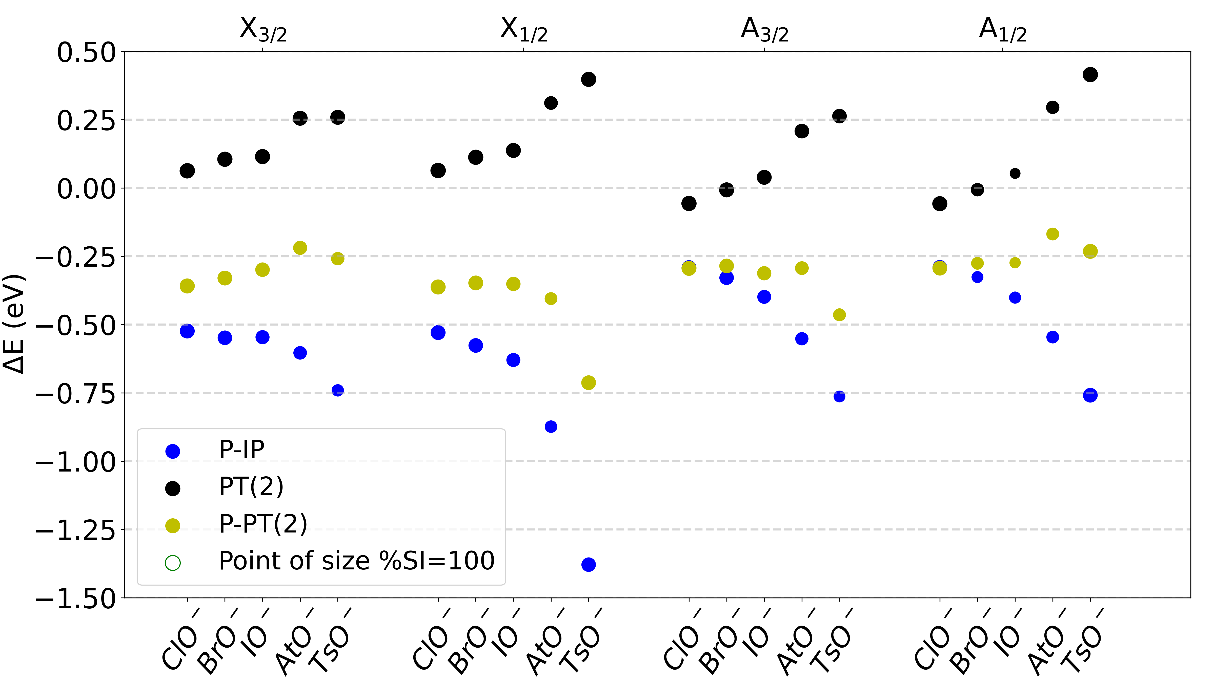
Figure 1: $\Delta E_{IP}$ values (in $\text{\,}\mathrm{eV}$) for the different approximate electronic structure methods considered here as a function of electronic state and halogen. Points have a size proportional to %SI (see Supplementary Information for the list of individual ionization energy values).

We observe that P-IP presents the worst results in terms of the absolute value of $\Delta E_{IP}$ among all three approximations considered, and the errors being all negative means that IPs are underestimated. For the $X_{3/2}$ state we see that the error is somewhat constant (around $-0.5\text{\,}\mathrm{eV}$) from chlorine to iodine, and slowly increases for astatine and tennessine to reach around $-0.75\text{\,}\mathrm{eV}$.

In qualitative terms, this is similar to what one sees for the PT(2)-IP case. For both spin-orbit split components of the excited state, we see a similar trend, but it differs slightly from PT(2)-IP case, since for the $A_{3/2}$ state there is a larger difference between astatine and tennessine. What is remarkable in P-IP is that for $X_{1/2}$ state there is a strong change in $\Delta E_{IP}$ when going from astatine to tennessine, with the error reaching $-1.38\text{\,}\mathrm{eV}$.

One element that may help understand the root of this behavior is the nature of this state : as discussed by Shee et al. (2018), in the EOM-IP-CCSD description of TsO, the $X_{1/2}$ state is predominantly made up by a configuration with 1h character, in which $\pi^{*}_{1/2}$ spinor ends up being singly occupied. However, there is also a contribution from a configuration with 2h1p character (on top of removing one electron from $\pi^{*}_{1/2}$, an electron from the doubly occupied $\sigma_{1/2}$ is placed on the empty $\sigma^{*}_{1/2}$ spinor) that is sufficiently large to affect energies by a few tenths of an $\text{\,}\mathrm{eV}$ in comparison to Fock-space coupled cluster results Shee et al. (2018).

In such a case P-IP turns out to be a poor approximation since it suppresses the ability of $\bar{H}_{DD}$ to account for the energetics of relaxation through the 2h1p configurations, though the nature of the $X_{1/2}$ state (spinors centered on tennessine, for which relaxation effects are potentially more important) may also play a role.

Case in point, the $\Delta E_{IP}$ values for the $A$ states of TsO are similar, even though EOM-IP-CCSD calculations indicate the $A_{1/2}$ state also has a non-negligible contribution with 2h1p character (the $\pi^{*}_{1/2}$ remains doubly occupied and two electrons are removed from the $\sigma_{1/2}$ and one place on $\sigma^{*}_{1/2}$) whereas the $A_{3/2}$ does not. But in constrast to the $X$ states, $A$ states are centered on oxygen.

Finally, it turns out that the approximation of the $\bar{H}_{DD}$ block in the P-PT(2)-IP method is compensated to some extent by the errors introduced by the approximate treatment of electron correlation. From chlorine to iodine, the differences are included in the limits: $\left[-0.36;\ -0.27\right]$$\text{\,}\mathrm{eV}$, in this case $\bar{\delta}=$0.34\text{\,}\mathrm{eV}$$ and $\sigma=$0.02\text{\,}\mathrm{eV}$$ for $X$ states and $\bar{\delta}=$0.29\text{\,}\mathrm{eV}$$, $\sigma=$0.01\text{\,}\mathrm{eV}$$ for $A$ states.

The standard deviations show us that the error is almost constant, with only the results for the $\Omega=1/2$ component of the ground state and to a lesser extend, the $\Omega=3/2$ component of the excited state of TsO deviating significantly from this trend. Paradoxically the most approximate method becomes, in this case, the most stable across the halogen monoxide series.

A final remark concerns the change in %SI for the different complexes and electronic states, shown in the Supplementary Information. We observe that there is no evident correlation between a particular value (i.e. whether a state is mono or multiconfigurational) and the magnitude of $\Delta E_{IP}$.

We do note, however, that PT(2)-IP are typically very close to that of the reference calculations, whereas P-IP values are usually smaller than the reference and PT(2)-IP ones, and P-PT(2)-IP values as expected fall in between PT(2)-IP and P-IP (though tend to be closer to the latter).

Taken together, these suggest that the approximation of $\bar{H}_{DD}$ does have a non-negligible impact on the nature of the wavefunction by favoring an increase in multiconfigurational character for the 1h contributions.

IV.1.2 Valence ionizations, potential energy curves

Apart from the investigation for ground-state equilibrium structures, we have also investigated the effect of the approximation on the potential energy curves for $X$ and $A$ states of the halogen monoxide radicals. As an example, we shown in figure 2 the results for the AtO species, as a representative of the overall trends. The curves for the other species as well as their equilibrium distances can be found in the Supplementary Information.

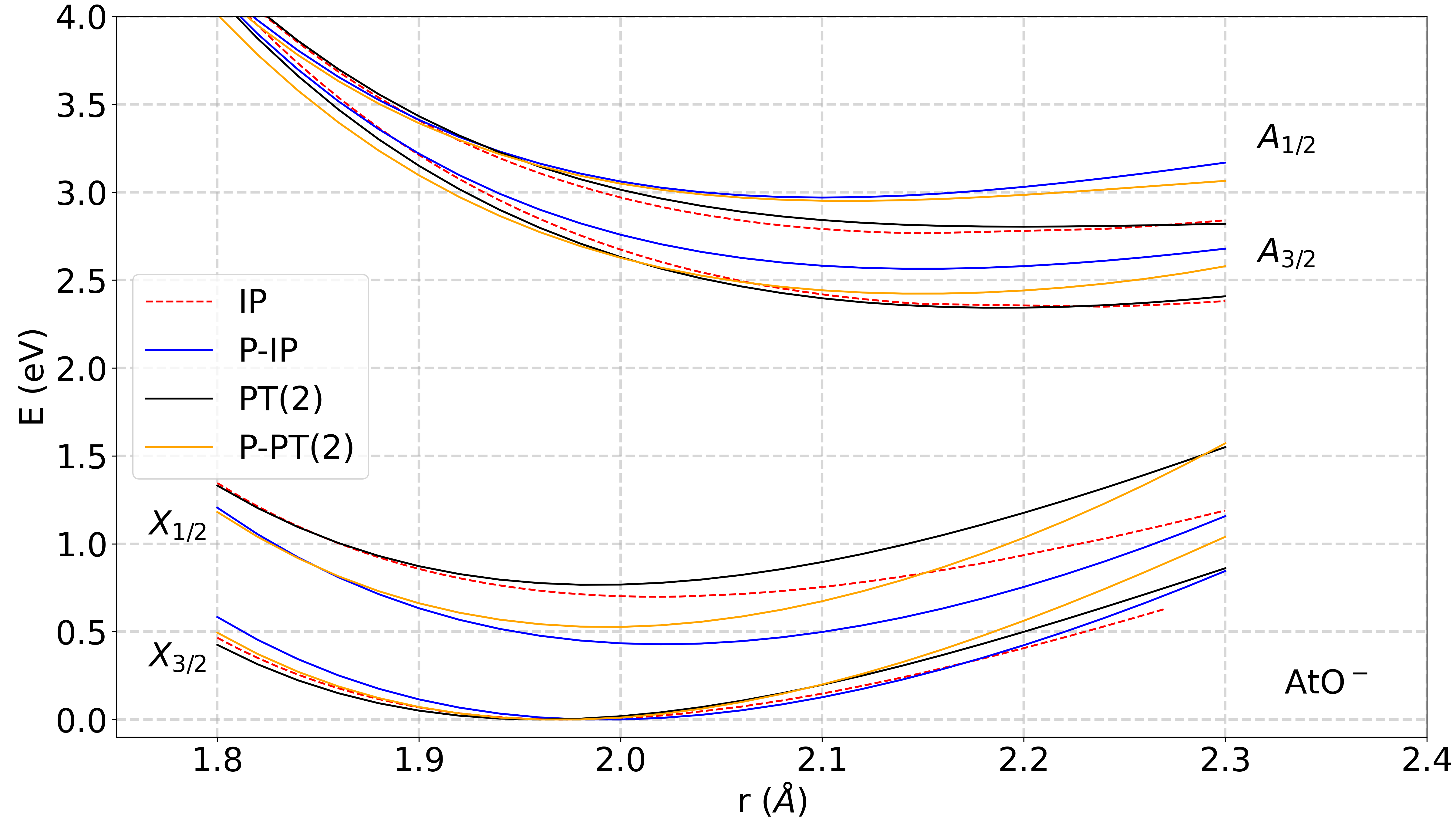
Figure 2: Potential energy curve for AtO (in $\text{\,}\mathrm{eV}$, shifted by the energy at the minimum of the $X_{3/2}$ state) as function of the X-O distance (r, in Å), for the reference method and the different approximations.

The first information from figure 2 is that PT(2)-IP (in black) shows very good agreement to the reference values (in red) for the $A$ states across the studied geometries. It also reproduces rather well the curves for the $X$ states up to the $X_{3/2}$ equilibrium structure; for larger internuclear distances, it starts to shift towards higher energies for both spin-orbit spit components, but the deviation with respect to the reference becomes more significant for the $X_{1/2}$ state than for the $X_{3/2}$ state.

Second, we see that the curves for the partition-based approaches (P-IP in blue and P-PT(2)-IP in yellow) are quite close to each other for internuclear distances shorther than the $X_{3/2}$ equilibrium structure, and start to separate out for larger distances; interestingly, P-PT(2)-IP energies tend to be higher than P-IP ones for the $X$ states, while the reverse is true for the $A$ states.

Taken together, these results hint that for halogen monoxides P-PT(2)-IP should not necessarily be more reliable than PT(2)-IP for obtaining spectroscopic constants, or investigating excited states for geometries away from the ground-state equilibrium. But whatever the case, they provide further evidence that P-IP is the least balanced of the three approximate methods under consideration.

From the graphs it is also interesting to notice that for the $X_{1/2}$ the P-PT(2)-IP curve goes to being closer to the P-IP curve for small internuclear distances to being closer to the PT(2)-IP for longer distances. However, this behavior is not observed for the other three states, indicating that the error cancellation that benefits the P-PT(2)-IP approach near the equilibrium structure of the ground state is not consistent across different structures.

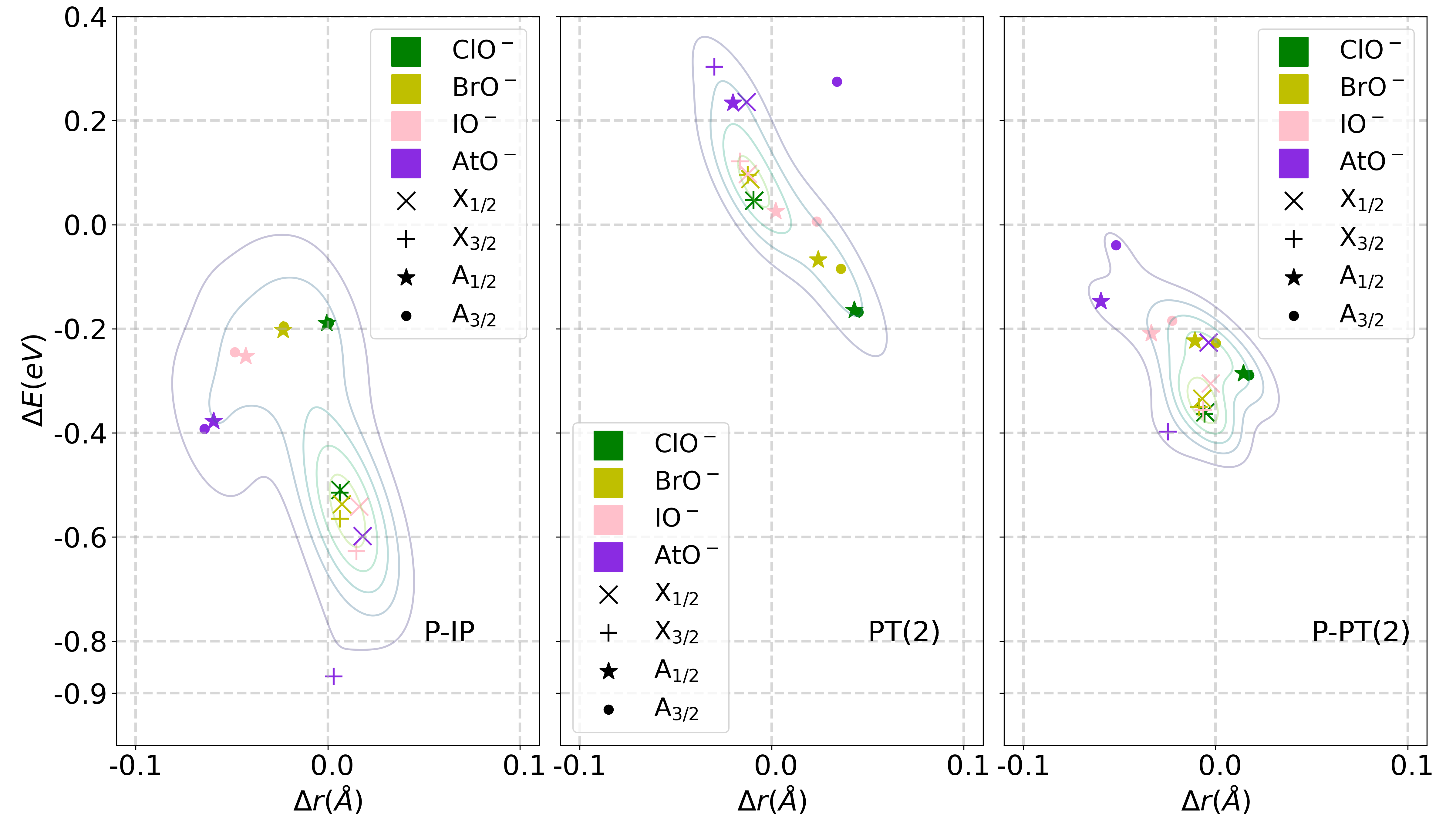
Figure 3: Difference in the PES minimums positions and energies $\Delta E$ (in $\text{\,}\mathrm{eV}$) w.r.t. $\Delta r$ (Å) for the 3 $\text{IP}_{\text{App}}$ and the 4 compounds. For reasons of readability : colors for compounds and symbols for states. The 4 different isodensities represented were calculated by a Gaussian kde algorithmSci , resp. in [-0.1; 0.1] ($\mathring{A}$), [-1.0; 0.4] ($\text{\,}\mathrm{eV}$) limits for $\Delta r$ and $\Delta E$.

To complement this comparison we provide in figure 3 a closer look at how both energetics and equilibrium structures compare to the reference values ($\Delta E$ and $\Delta_{r}$, respectively) for the different species. From this figure we clearly see that results for P-IP are rather dispersed both in energetics and geometries.

The results for PT(2)-IP on the other hand cluster around the reference values, but not in a very homogeneous way for different species. A similar clustering is seen for P-PT(2)-IP, with the systematic error for energies which has been discussed above comparison to PT(2)-IP being clearly seen. We also observe that for chorine, bromine and iodine, P-PT(2)-IP results are more compactly clustered together than for PT(2)-IP (all values are included in a zone of $\pm$$0.1\text{\,}\mathrm{eV}$ and $\pm$$0.025\text{\,}\mathrm{\SIUnitSymbolAngstrom}$).

The difference between PT(2)-IP and IP can be explained by a poorer description of the ground state by this approximation Gwaltney, Nooijen, and Bartlett (1996). A correction can be made by comparing the CCSD correlation energies with respect to MP2. We corrected our results by the difference between these two energies (relative to their respective minima) along the dissociation curve; this sometimes seems to improve the results but without a general conclusion appearing.

This compensation method can be interesting in the explanation but not very advantageous for obtaining the energies, the purpose of PT(2)-IP and P-PT(2)-IP being to avoid doing CCSD calculations. This correction could also have been made in the previous study on XO^- but a change in the baseline only leads to a change in the mean and not in the standard deviation (as the distance is the same in both IP methods).

So far we have discussed the errors for the individual excited state energies, however, it is also crucial to examine how the methods represent the energy differences between electronic states. If such energy differences are correctly described it becomes possible to investigage electronic transitions. Since in our discussion of the potential energy curves we have established that the errors for the different approximate methods are not constant, we restrict ourselves to a comparison around the ground-state equilibrium structure (the Franck-Condon zone).

Concerning the errors in transition energies, these are shown in figure 4; there, we take the lowest state ($X_{3/2}$) as reference. As the first transition is between the spin-orbit components of the ground state, for chlorine and bromine results are essentially the same. For the two other compounds, the error increases for P-IP, for PT(2)-IP, the energies are correct with deviation smaller than $0.1\text{\,}\mathrm{eV}$. For P-PT(2)-IP, the error remains small up to iodine for which the error is $-0.05\text{\,}\mathrm{eV}$.

For the following two transitions ($A_{3/2}$-$X_{3/2}$and $A_{1/2}$-$X_{3/2}$), for the same IP_App and the same compound, the errors are essentially the same. P-IP overestimates the energies, PT(2)-IP underestimates them but becomes more reliable for as systems become heavier (e.g.  from ClO^- to AtO^-). P-PT(2)-IP shows a more systematic behavior for the transitions between $\Omega=3/2$ than between $\Omega=3/2$ and $\Omega=1/2$ states.

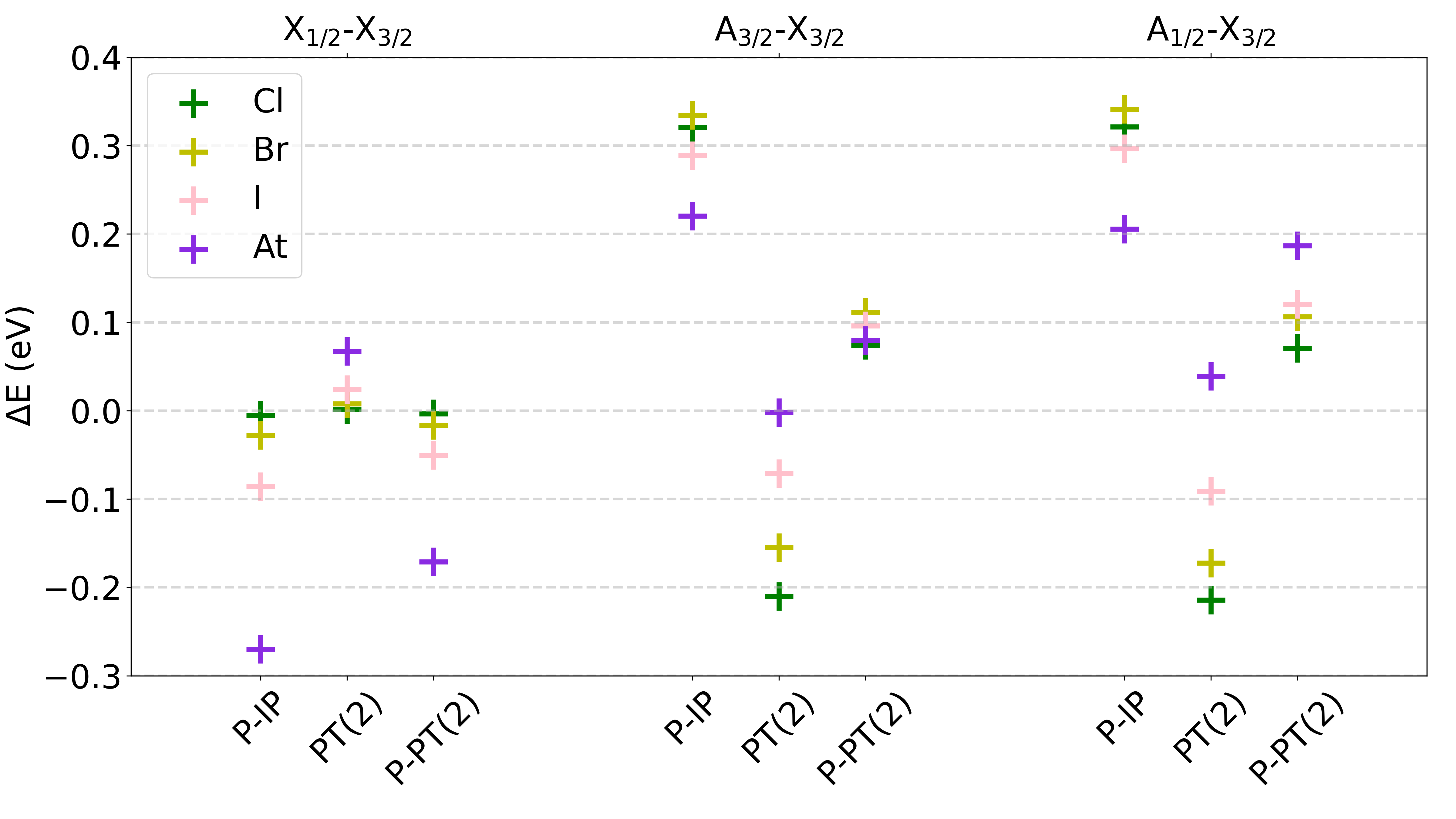
Figure 4: Error in transition energies : $\Delta$$\text{IP}_{\text{App}}$-$\Delta$IP (in $\text{\,}\mathrm{eV}$), for all XO^- and $\text{IP}_{\text{App}}$s (see Supplementary Information for values).

IV.1.3 Core ionizations

On order to avoid complexifying the notation in what follows, we will continue to employ the same acronyms for ther reference and approximate methods as done for valence ionizations, but for the results all approximated methods ($\text{IP}_{\text{App}}$) and the reference EOM-CCSD results (IP), it will be implicit that they were obtained the CVS approximation Halbert et al. (2021).

Apart from those, since for highly symmetric systems such as HCl, HBr and I^- the DIRAC implementation can be used to carry out a complete diagonalization (that is, obtain all possible states from the EOM-CCSD matrix without invoking the CVS approximation), we take the opportunity to present these results (denoted by the shorthand full-IP) and compare them to IP ones, thus extending our previous comparison Halbert et al. (2021).

Our results are shown in Table 2 for K- and L-edges of HCl, the M-edges of HBr, and the K-, L- and M-edges of I^-. In it, we present the full-IP and IP energies along their respective differences (denoted by $\Delta_{f}$), as well as the $\Delta E_{IP}$ values gauging the difference between approximate methods and the reference IP results.

Before addressing the results for approximate methods, we see from table 2 that the effect of the CVS approximation is rather small, with $\Delta_{f}$ values being usually of a few tenths of an $\text{\,}\mathrm{eV}$ for most edges–including highly energetic ones such as the I^- K-edge–with a few exceptions that we had identified previously Halbert et al. (2021). We also see that for molecular systems, the hydrogen-halogen bond slightly lifts the degeneracies that are expected for each of the edges if the systems were spherically symmetric, but for these systems these splittings are not particuarly important. Taken together, these results attest to the reliability of the CVS approximation, for the discussion that follows.

Table 2: Ionization energies (in $\text{\,}\mathrm{eV}$) for HCl (K- and L-edges), HBr (M-edges) and I^- (K-, L- and M-edges) for the complete diagonalization of the EOM-IP-CCSD Hamiltonian (full-IP) and for the CVS approximation (IP), as well as their difference ($\Delta_{f}$, in $\text{\,}\mathrm{eV}$). Energy differences ($\Delta E_{IP}$, in $\text{\,}\mathrm{eV}$) between approximate methods and IP. We note that %SI $\text{IP}_{\text{App}}$ are included in the range [87%; 88%], [89%; 91%] and [88%; 92%] respectively for HCl, HBr and I^-. The differences between labels $(a)$, $(b)$ and $(c)$ denote the splitting of states due to the deviation from spherical symmetry in the presence of the hydrogen atom.

	full-IP	CVS-IP		$\Delta E_{IP}$
T	Ef	EIP	$\Delta_{f}$	P-IP	PT(2)-IP	P-PT(2)-IP
	HCl
$K$	2835.46	2835.76	0.30	-0.45	0.23	-0.20
$L_{1}$	280.25	280.27	0.02	-0.14	0.12	-0.01
$L_{2}$	209.66	209.59	-0.07	-0.06	0.13	0.09
$L_{3}(a)$	208.02	207.93	-0.09	-0.15	0.13	0.09
$L_{3}(b)$	207.94	207.84	-0.10	-0.06	0.13	0.08
	HBr
$M_{2}$	200.77	200.92	0.16	-1.15	0.15	-0.85
$M_{3}(a)$	194.21	194.00	-0.21	-1.13	0.15	-0.83
$M_{3}(b)$	194.15	193.84	-0.31	-1.13	0.14	-0.84
$M_{4}(a)$	78.03	78.13	0.10	-1.15	0.23	-0.78
$M_{4}(b)$	77.84	77.90	0.06	-1.16	0.23	-0.80
$M_{5}(a)$	77.00	77.05	0.06	-1.13	0.23	-0.77
$M_{5}(b)$	77.01	76.93	-0.08	-1.13	0.23	-0.78
$M_{5}(c)$	76.88	76.74	-0.13	-1.14	0.22	-0.79
	I-
$K$	33290.63	33290.72	0.09	-5.77	1.27	-4.25
$L_{1}$	5209.13	5209.29	0.16	-4.35	1.02	-3.11
$L_{2}$	4866.09	4867.68	1.59	-4.67	1.07	-3.37
$L_{3}$	4567.06	4567.67	0.61	-4.53	1.06	-3.25
$M_{1}$	1078.43	1078.27	-0.16	-2.25	0.72	-1.41
$M_{2}$	937.25	936.37	0.12	-2.31	0.75	-1.44
$M_{3}$	878.64	878.57	-0.06	-2.21	0.74	-1.36
$M_{4}$	631.93	631.67	-0.26	-2.42	0.80	-1.50
$M_{5}$	618.89	619.81	0.91	-2.39	0.79	-1.48

Turning now to the performance of the approximate methods, we begin with the results HCl. We observe, for PT(2)-IP a very homogeneous error for the L-edge at around $0.13\text{\,}\mathrm{eV}$, and a slightly larger error ($0.23\text{\,}\mathrm{eV}$) for the K-edge. For P-IP, we see errors of opposite sign compared to PT(2)-IP, indicating once more that the reference values are underestimated. More interestingly they are, in absolute value, twice as large for the K-edge, comparable for the $L_{1}$- and $L_{3}(a)$- edges, and slightly smaller for the other edges.

In the P-PT(2)-IP, we see a pattern of error cancellation which is very similar to that found for the valence ionization, though since there are much more significant differences between PT(2)-IP and P-IP for the K-edge than for the others, we see a much larger value of $\Delta E_{IP}$.

Moving on to HBr, we only compare the M-edge which is of similar or lower energy than the K- and L-edges of HCl. Perhaps unsurprisingly, for PT(2)-IP we see $\Delta E_{IP}$ values with are similar to, or slighlty larger than those for HCl, attesting to the very systematic nature of this approximation. For P-IP we also have quite systematic errors, but they underestimate the reference more significantly than for HCl, and now in absolute value the $\Delta E_{IP}$ are nearly $1\text{\,}\mathrm{eV}$ larger than for PT(2)-IP; and consequently P-PT(2)-IP are also affected and in absolute value $\Delta E_{IP}$ are sigificantly larger than for PT(2)-IP.

A similar trend emerges for I^-, with PT(2)-IP showing a tendency to overestimate the reference (by about $1\text{\,}\mathrm{eV}$), with $\Delta E_{IP}$ which are comparable within each edge. The P-IP and PT(2)-IP approaches also show $\Delta E_{IP}$ values which are very similar within each edge, but both show $\Delta E_{IP}$ values which in absolute terms are significatly (between two to five times) larger than the PT(2)-IP values.

In figure 5 we provide a graphical representation of $\Delta E_{IP}$ shown in table 2 above for each of the approximate methods, adding to it (red) a measure of the non-additivity (NA) of the partition and second-order approximations:

$$\mathrm{NA}=\Delta E_{IP}(\mathrm{PT(2){}})-\left[\Delta E_{IP}(\mathrm{P-PT(2){}})-\Delta E_{IP}(\mathrm{P-IP{}})\right],$$ (22)

from which we see that there is a small non-additivity, that is slightly larger for the K and L edges with respect to the M edges.

To explain the processes behind these differences, one should first recall that as discussed elsewhere (see e.g. Halbert et al. (2021) and references therein), for the determination of core ionization energies, the contribution to the electronic states’ energies of relaxation effects due to the creation of the core hole can be equally or more important than electron correlation effects as discussed by South et al. (2016).

Furthermore, relaxation will be increasingly more important as one probes more energetic edges. With that, electronic structure methods that insufficiently account for relaxation (for example, using Koopmans theorem to approximate ionization energies by the absolute value of orbital energies) will in general largely overestimate core binding energies and show larger discrepancies from experiment for more energetic edges than for less energetic ones (by several tens of $\text{\,}\mathrm{eV}$ depending on the case).

Methods such as EOM-CCSD on the other hand have shown to be capable of accounting for a significant part of relaxation, and when combined with corrections for quantum electrodynamics effects and the Breit interaction are taken into account, one can obtain energies in agreement with experiment to within about 1-2 $\text{\,}\mathrm{eV}$ Halbert et al. (2021); Opoku, Toubin, and Gomes (2022), and show fairly constant errors for different edges.

In view of these results from the literature and our results above, in which we see fairly constant $\Delta E_{IP}$ values for PT(2)-IP (but more energetic edges showing slightly larger values than less energetics ones), while at the same time observing a net increase in the magnitude of $\Delta E_{IP}$ for both P-IP and P-PT(2)-IP as one goes towards (a) heavier elements; and (b) more energetic edges, we are led to the conclusion that for core ionizations PT(2)-IP does a better job at accounting for relaxation than the partition-based approaches, due to the approximation to the $\bar{H}_{DD}$ block in the latter two.

That said, it is important to recall that all $\Delta E_{IP}$ values shown here remain significant smaller than what would be the case if cruder approximations were employed (e.g. Koopmans theorem), meaning that these approximate methods (and in particular PT(2)-IP and P-PT(2)-IP, due to their more modest computational cost) would remain of interest for the calculation of core ionizations.

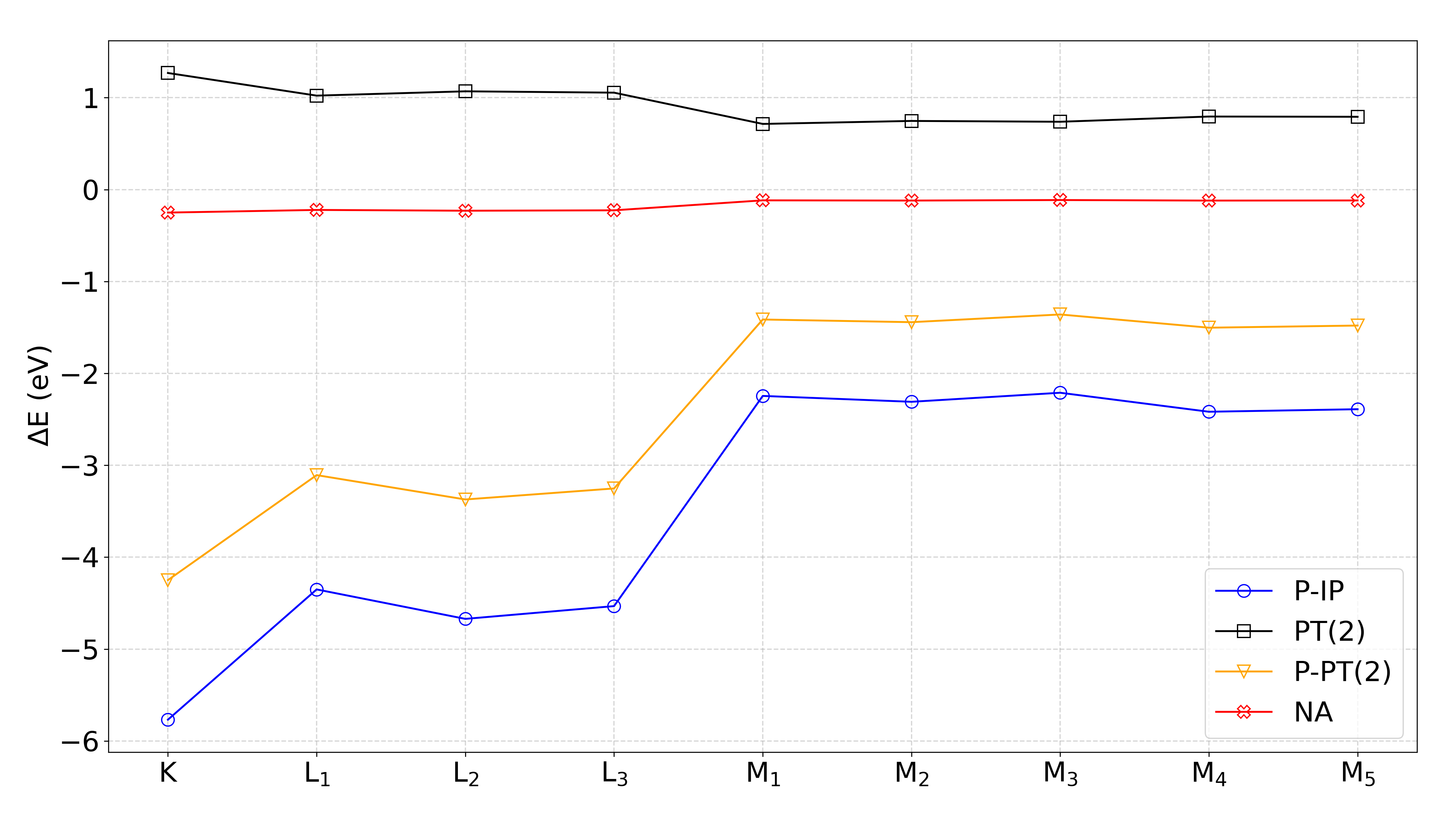
Figure 5: Values of $\Delta E_{IP}$ (in $\text{\,}\mathrm{eV}$) for the K-, L- and M- edges of I^- for the PT(2)-IP, P-IP and P-PT(2)-IP approximations, as well as a measure of the non-additivity (NA) of the partition and second-order approximations.

Finally, we note that for all ionizations considered, we have %SI around [87%; 88%] for HCl, [89%; 91%] for HBr and [88%; 92%] for I^-, meaning that for all methods and systems we have been able to compare ionized states whose wavefunctions are dominated by the same ionized determinant. It is also interesting to see that for the core spectra of these species we did not see the partition-based approaches increasing the states’ multideterminantal character.

IV.2 Electronic Affinities

Addressing now electron affinities, we summarize our results in table 3. We see that for all systems considered (I${}_{3}^{-}$, CH₂IBr and CH₂I₂), we have rather small and uniform errors for all approximations, so it is actually quite difficult to decide which one shows better performance as done for ionization energies. That said, we still see that PT(2)-EA still appears to be somewhat more systematic than the partition-based approaches P-EA and P-PT(2)-EA.

For these systems most electron affinities are positive and relatively large, corresponding to situation in which we have metastable states. For these cases, we see that the error introduced by the approximations are rather negligible in comparison to the electron affinities themselves.

For CH₂IBr and CH₂I₂, on the other hand, the first electron affinity is negative, denoting bound states that are nevertheless not very stable–$-0.03\text{\,}\mathrm{eV}$ for CH₂IBr and $-0.33\text{\,}\mathrm{eV}$ for CH₂I₂ respectively. We see that all of our approximated methods tend to underestimate the energies of these bound states. That makes them yield first electron attachments states which are also bound, and therefore qualitatively in line with EOM-CCSD, though slightly more stable than the latter.

These results underscore the fact that, by introducting approximations one invariably loses in accuracy, and consequently in predictive power when tiny energy differences are involved. This serves as a reminder of the importance of attempting to investigate such subtle effects with a range of methods of verying degrees of accuracy to verify whether computationally less expensive methods are sufficiently accurate.

It is noteworthy that the %SA are sometimes over 90%, but also as low as 50%, indicating the presence of at least one or more configurations, though the values are very similar across all methods for each of the individual electronic states.

Table 3: Electron affinities and $\Delta E_{EA}$ values (in $\text{\,}\mathrm{eV}$) as well as %SA values for selected low-lying states of the I${}_{3}^{-}$, CH₂IBr and CH₂I₂ molecules.

	EA		P-EA		PT(2)-EA		P-PT(2)-EA
T	E	%SA	%SA	$\Delta E_{EA}$	%SA	$\Delta E_{EA}$	%SA	$\Delta E_{EA}$
	I${}_{3}^{-}$
EA1	2.51	76	76	-0.02	75	-0.01	74	-0.05
EA2	3.65	77	77	0.01	76	0.01	75	0.01
EA3	3.88	94	94	0.01	94	0.02	95	0.03
EA4	4.39	96	96	0.01	96	0.00	96	0.01
	CH2IBr
EA1	-0.03	52	53	-0.04	52	-0.06	53	-0.08
EA2	0.45	66	70	0.00	67	-0.01	70	-0.00
EA3	0.86	97	97	0.01	97	-0.01	97	0.00
EA4	0.99	87	85	-0.00	86	-0.01	85	-0.01
EA5	1.62	70	69	0.01	68	-0.01	67	0.01
EA6	1.92	52	49	0.00	55	-0.01	48	-0.00
	CH2I2
EA1	-0.33	48	50	-0.06	48	-0.06	49	-0.10
EA2	0.41	57	60	0.01	58	-0.01	60	0.00
EA3	0.75	83	81	-0.02	82	-0.01	80	-0.02
EA4	0.86	98	98	0.01	98	-0.01	98	0.00
EA5	1.49	87	86	0.01	86	-0.00	85	0.01
EA6	1.70	67	62	-0.01	65	-0.01	61	-0.01

IV.3 Excitation Energies

As a conclusion, we focus on the calculation of excitations energies with our approximate methods. Our results are reported on table 4 for the triiodide I${}_{3}^{-}$ and dihalomethane CH₂I₂ species.

Starting with the triiodide results, we see that our three approaches work rather well as far as the standard deviation of $\Delta E_{EE}$ values is concerned-these are all small, meaning that that the errors for P-EE and PT(2)-EE are shifts of roughly $0.27\text{\,}\mathrm{eV}$ for the first (meaning it it overestimates the reference values) and nearly zero for the second. Due to this behavior for P-PT(2)-EE in this particular example the results are nearly identical to those of P-EE and there are no significant error cancellations, unlike the case if ionization energies as pointed out in the case of ionization energies.

One thing to note is that in cases in which states are nearly degenerate such as $\left\{1_{g};\ 0^{-}_{u};\ 1_{u}\right\}$, the approximate methods have a difficult time in placing them in the same order as found in EOM-CCSD (see numbers in bold on table 4). Furthermore, we note the presence of non-standard values for the first $1_{g}$ and $1_{u}$ by PT(2)-EE and P-PT(2)-EE. Indeed, while PT(2)-EE presents a difference of at most $0.01\text{\,}\mathrm{eV}$ in absolute value, the error for this level is $0.11\text{\,}\mathrm{eV}$. The same is true for P-PT(2)-EE which goes from an error of $0.27\text{\,}\mathrm{eV}$ to $0.37\text{\,}\mathrm{eV}$. These differences to EOM-CCSD are in line with limitations pointed out above for electron affinities.

Similar trends are found for CH₂I₂. For this system, standard deviations are once again satisfactory, of the order of $0.2\text{\,}\mathrm{eV}$, with the averages are respectively $0.31\text{\,}\mathrm{eV}$, $-0.07\text{\,}\mathrm{eV}$ and $0.25\text{\,}\mathrm{eV}$ for P-EE, PT(2)-EE and P-PT(2)-EE respectively. This means that we observe very systematic but nevertheless larger overestimation P-EE, and now a slight underestimation by PT(2)-EE, which is actually the opposite trend found for for ionization energies, but that means that P-PT(2)-EE again profits from error calcellation between the second-order and partition approximations. As in the case of electron affinities, we find that overall %EE values are also very similar between different approximate methods, in spite of the fluctuations from state to state.

Finally, for the comparison with CASPT(2) results for I${}_{3}^{-}$ Gomes et al. (2010) and CH₂I₂ by Liu et al. (2007), we see that in terms of the mean error the PT(2)-EE performs better than CASPT2 for both molecules, whereas P-EE and P-PT(2)-EE shows a simular behavior. However, in contrast to our methods, the $\Delta E_{EE}$ values for CASPT2 vary much more significantly from state to state, as reflected in its much larger standard deviations.

This tendency of varying $\Delta E_{EE}$ for different excited states had already been identified by Gomes et al. (2010) and Shee et al. (2018), but also in other benchmarks for heavy elements such as those by Tecmer et al. (2011) and Tecmer et al. (2014). We consider it a significant advantage of the approximate methods over CASPT2 that former conserve such near constant difference to EOM-CCSD values. This characteristic reduces the risk of incorrectly ordering electronic states, enhancing the reliability of the approximate methods in this regard.

Table 4: Excitation energies and $\Delta E_{EE}$ values (in $\text{\,}\mathrm{eV}$) as well as %SE values for selected low-lying excited states of the I${}_{3}^{-}$ and CH₂I₂ molecules. In bold we denote electronic states whose order has been inverted in approximate calculations with respect to the reference EOM-CCSD results. Here $\bar{x}$ and $\sigma$ denote the mean error over all excited states considered for a particular species and the standard deviation, respectively. CASPT2 values from Gomes et al. (2010) for I${}_{3}^{-}$ and from Liu et al. (2007) for CH₂I₂ are also provided for comparison.

	EE		P-EE		PT(2)-EE		P-PT(2)-EE		CASPT2
T	EE	%SE	%SE	$\Delta E_{EE}$	%SE	$\Delta E_{EE}$	%SE	$\Delta E_{EE}$	E	$\Delta E_{EE}$
	I${}_{3}^{-}$
2g	2.25	43	45	0.27	43	0.00	45	0.27	2.24	-0.01
1g	2.38	23	24	0.25	23	0.11	24	0.37	2.32	-0.06
0${}_{u}^{-}$	2.38	41	42	0.27	41	0.00	42	0.27	2.47	0.09
1u	2.38	46	47	0.25	46	0.11	47	0.37	2.47	0.09
0${}_{g}^{-}$	2.84	21	22	0.27	22	0.00	22	0.28	2.76	-0.08
0${}_{g}^{+}$	2.89	21	22	0.27	21	0.00	22	0.27	2.82	-0.07
1g	3.07	41	43	0.28	41	0.01	43	0.28	2.85	-0.22
2u	3.33	48	49	0.26	48	-0.01	49	0.24	3.10	-0.23
1u	3.42	48	49	0.26	48	-0.01	49	0.25	3.11	-0.31
$\mathbf{0_{u}^{+}}$	3.67	18	19	0.24	17	-0.01	19	0.23	3.52	-0.15
2g	4.08	24	24	0.27	24	-0.01	24	0.26	3.98	-0.10
0${}_{u}^{-}$	4.10	42	43	0.29	42	-0.01	43	0.28	3.79	-0.31
1g	4.18	47	48	0.28	47	-0.01	49	0.27	4.06	-0.12
1u	4.22	40	41	0.30	40	-0.00	40	0.29	3.80	-0.42
$\mathbf{0_{u}^{+}}$	4.49	15	16	0.24	15	0.00	17	0.24	4.51	0.02
0${}_{g}^{-}$	4.69	20	21	0.30	20	-0.01	21	0.29	4.51	-0.18
0${}_{g}^{+}$	4.70	20	21	0.30	20	-0.01	21	0.29	4.53	-0.17
1g	4.90	40	36	0.30	40	0.01	26	0.33	4.60	-0.30
$\bar{x}$				0.27		0.01		0.28		-0.14
$\sigma$				0.02		0.04		0.04		0.14
	CH2I2
a	3.60	20	21	0.29	20	-0.07	21	0.23	3.76	0.16
b	3.62	20	20	0.29	20	-0.07	20	0.23	3.78	0.16
a	3.62	20	21	0.29	20	-0.06	21	0.23	3.78	0.15
b	3.84	16	17	0.30	15	-0.07	16	0.23	4.03	0.19
a	3.87	19	19	0.29	19	-0.07	19	0.23	4.27	0.40
b	3.94	13	13	0.31	12	-0.08	13	0.24	4.27	0.33
a	3.99	16	17	0.30	16	-0.08	17	0.23	4.31	0.32
b	4.06	16	16	0.31	16	-0.07	16	0.24	4.38	0.32
b	4.22	18	19	0.30	18	-0.06	19	0.25	4.50	0.28
a	4.32	15	16	0.31	15	-0.07	16	0.24	4.60	0.28
b	4.35	15	15	0.31	15	-0.06	15	0.26	4.62	0.27
a	4.49	15	15	0.31	15	-0.07	16	0.25
b	4.63	15	15	0.33	15	-0.07	15	0.27
a	4.68	17	17	0.35	17	-0.06	18	0.30
b	4.74	15	14	0.34	15	-0.07	15	0.28
a	4.91	14	15	0.36	15	-0.06	15	0.30
$\bar{x}$				0.31		-0.07		0.25		0.26
$\sigma$				0.02		0.01		0.02		0.08

V Conclusion

In this manuscript we have detailed a pilot impementation of three approximate methods based on the relativistic EOM-CCSD method–the partitioned EOM-CCSD (P-EOM-CCSD), the second-order approximation to EOM-CCSD (EOM-MBPT(2)) and the partitioned EOM-MBPT(2)(P-EOM-MBPT(2))–and applied them to a number of benchmark systems to assess how they compare with respect to the original EOM-CCSD for core and valence ionization, electron affinities and valence excitation energies.

These approximated methods have been shown to provide, for the most part, sufficiently accurate results with respect to the reference EOM-CCSD calculations. As a general rule, EOM-MBPT(2) has shown to overestimate reference values in a very systematic manner for ionizations and electron affinities, often by no more than a few tenths of $\text{\,}\mathrm{eV}$ for valence ionizations and somewhat less for electron affinities, and at most around 1-2 $\text{\,}\mathrm{eV}$ for core ionizations (employing the core-valence separation method). For excitation energies on the other hand it tends to slighly underestimate the EOM-CCSD results.

Conversely, the P-EOM method tends to systematically underestimate EOM-CCSD results for ionizations and electron affinities, while overestimating excitation energies. For ionizations and excitations, magnitude of the errors is in general larger than those for the EOM-MBPT(2) method, but rather similar for electron affinities. We have found however that for ionization processes in which relaxation effects brought about by 2h1p configurations are important (here, the valence ionization of tennessine monoxide, and the core ionizations of halogen-containing systems), the approximation underlying the P-EOM method (discarding all off-diagonal elements of $\bar{H}_{DD}$ and approximating the diagonal by orbital energy differences) degrades the reliability of the method, and results differ from the reference EOM-CCSD the more such relaxation effects are important.

Because it combines both approximations, the P-EOM-MBPT(2) shows a behavior that is intermediate between EOM-MBPT(2) and P-EOM due to error cancellation. It should be said however that the method does show interesting and stable systematic errors, and will suffer less of a performance degradation that P-EOM even for cases which are particularly difficult for the latter such as the valence ionization of tennesine oxide.

Another finding is that for ionizations P-EOM, and to a lesser extent P-EOM-MBPT(2), seem to somewhat reduce the monodeterminantal nature of ionized states, compared to the EOM-CCSD and EOM-MBPT(2) calculations, though we consider these to be a consequence of the partitioned approximation rather than an underlying cause for differences in performance. This point requires investigations on a broader class of complexes, that goes beyond the scope of this work.

With respect to their behavior across different structures, our investigation of the potential energy curves for the spin-orbit split ground and first excited states of halogen monoxides shows that all of these methods have different error cancellation patterns in different regions of the potential energy curves, and therefore should be used with caution. That said, the EOM-MBPT(2) and P-EOM-MBPT(2) methods have shown to yield relatively small errors in equilibrium bond lenghts for ClO, BrO and IO, with a small advantage for P-EOM-MBPT(2), though for AtO the reverse appears to be true.

With that, EOM-MBPT(2) seems to be a good first alternative to EOM-CCSD among the methods considered for carrying out exploratory calculations for valence and core properties on systems across the periodic table, followed by P-EOM-MBPT(2). On our view P-EOM does not seem to show a very interesting performance to cost ratio, especially for heavy and superheavy elements and should therefore be avoided, unless additional evidence for more molecular systems demonstrates other situations in which P-EOM fares as well or better than EOM-MBPT(2) or P-EOM-MBPT(2).

Furthermore, we observe that in the limited comparisons to CASPT2 for excitation energies, EOM-MBPT(2) shows overall better (and more systematic) agreement to EOM-CCSD while P-EOM-MBPT(2) results deviate from EOM-CCSD also in a more systematic way than CASPT2, though in absolute values their errors are comparable to CASPT2. This suggests these approximate EOM methods presented here can be viable alternatives to CASPT2 for investigating the spectroscopy of molecules with a single-reference ground states.

As a perspective for this work we have the implementation and subsequent exploration of additional approximate methods, such as the CC2 and EOM-CC2, in the simulation of heavy elements systems. There is a need for economical approaches for exploring (core) excited states of heavy element systems, which by denfinition contain many more inner electrons than first or second-row systems, but at the same time little if any knowledge on how these approaches will behave in such cases. These efforts are to be carried out as part of our further development of the ExaCorr code in DIRAC, which lifts many of the limitations of the RELCCSD module employed here for the treatment of larger molecular systems.

Appendix A Equations for approximated methods

Note that for the following equations : Internal sommations have been omitted and $P_{-}(pq)$ is a permutation operator : $P_{-}(pq)g(\dots,p,q,\dots)=g(\dots,p,q,\dots)-g(\dots,q,p,\dots)$.

As an exemple of the link between the following equations and the $\sigma$ vector used in the Davidson procedure, and Core-Valence-Separation (eq.12) we have (see Shee et al. (2018)):

$$\sigma_{i}^{a} =[\bar{H}_{SS}\mathcal{R}]^{a}_{i}+[\bar{H}_{SD}\mathcal{R}]^{a}_{i}$$ (23)

$$\sigma_{ij}^{ab} =[\bar{H}_{DS}\mathcal{R}]_{ij}^{ab}+[\bar{H}_{DD}\mathcal{R}]_{ij}^{ab}$$ (24)

A.1 MBPT(2) - EOM-EE

$$[\bar{H}_{SS}\mathcal{R}]^{a}_{i}= +{\color[rgb]{0,0,0}\bar{F}^{a}_{e}}r^{e}_{i}-{\color[rgb]{0,0,0}\bar{F}^{m}_{i}}r^{a}_{m}+{\color[rgb]{0,0,0}\mathcal{W}^{ma}_{ei}}r^{e}_{m}$$ (25)

$$[\bar{H}_{SD}\mathcal{R}]^{a}_{i}= +\bar{F}^{m}_{e}r^{ea}_{mi}+\frac{1}{2}\mathcal{W}^{am}_{ef}r^{ef}_{im}-\frac{1}{2}\mathcal{W}^{mn}_{ie}r^{ea}_{mn}$$ (26)

$$[\bar{H}_{DS}\mathcal{R}]_{ij}^{ab}= -P_{-}(ab){\color[rgb]{0,0,0}\mathcal{W}^{am}_{ij}}r^{b}_{m}+P_{-}(ij){\color[rgb]{0,0,0}\mathcal{W}^{ab}_{ej}}r^{e}_{i}$$

$$+P_{-}(ab)\left({\color[rgb]{0,0,0}V^{bm}_{fe}}r^{e}_{m}\right)t^{af}_{ij}{\color[rgb]{0,0,0}-}P_{-}(ij)\left({\color[rgb]{0,0,0}V^{nm}_{je}}r^{e}_{m}\right)t^{ab}_{in}$$ (27)

$$[\bar{H}_{DD}\mathcal{R}]_{ij}^{ab}= +P_{-}(ab){\color[rgb]{0,0,0}\bar{F}^{b}_{e}}r^{ae}_{ij}-P_{-}(ij){\color[rgb]{0,0,0}\bar{F}^{m}_{j}}r^{ab}_{im}$$

$$+\frac{1}{2}{\color[rgb]{0,0,0}\mathcal{W}^{mn}_{ij}}r^{ab}_{mn}+P_{-}(ab)P_{-}(ij){\color[rgb]{0,0,0}\mathcal{W}^{mb}_{ej}}r^{ae}_{im}$$

$$-\frac{1}{2}P_{-}(ab)\left(V^{nm}_{fe}r^{ea}_{mn}\right)t^{fb}_{ij}-\frac{1}{2}P_{-}(ij)\left(V^{nm}_{fe}r^{fe}_{jm}\right)t^{ab}_{in}$$

$$+\frac{1}{2}{\color[rgb]{0,0,0}\mathcal{W}^{ab}_{ef}}r^{ef}_{ij}$$ (28)

A.2 MBPT(2) - EOM-IP

$$[\bar{H}_{SS}\mathcal{R}]_{i} =-{\color[rgb]{0,0,0}\bar{F}^{m}_{i}}r_{m}$$ (29)

$$[\bar{H}_{SD}\mathcal{R}]_{i} =+\bar{F}^{m}_{e}r^{e}_{mi}-\frac{1}{2}\mathcal{W}^{mn}_{ie}r^{e}_{nm}$$ (30)

$$[\bar{H}_{DS}\mathcal{R}]_{ij}^{a} ={\color[rgb]{0,0,0}-}{\color[rgb]{0,0,0}\mathcal{W}^{am}_{ij}}r_{m}$$ (31)

$$[\bar{H}_{DD}\mathcal{R}]_{ij}^{a} =-P_{-}(ij){\color[rgb]{0,0,0}\bar{F}^{m}_{j}}r^{a}_{im}+{\color[rgb]{0,0,0}\bar{F}^{a}_{e}}r^{e}_{ij}+{\color[rgb]{0,0,0}\mathcal{W}^{mn}_{ij}}r^{a}_{mn}$$

$$+P_{-}(ij){\color[rgb]{0,0,0}\mathcal{W}^{am}_{ie}}r^{e}_{mj}-\frac{1}{2}\left(V^{mn}_{ef}r^{f}_{nm}\right)t^{ae}_{ij}$$ (32)

A.3 MBPT(2) - EOM-EA

$$[\bar{H}_{SS}\mathcal{R}]^{a} =+{\color[rgb]{0,0,0}\bar{F}^{a}_{e}}r^{e}$$ (33)

$$[\bar{H}_{SD}\mathcal{R}]^{a} =+\bar{F}^{m}_{e}r^{ea}_{m}+\frac{1}{2}\mathcal{W}^{am}_{ef}r^{fe}_{m}$$ (34)

$$[\bar{H}_{DS}\mathcal{R}]_{i}^{ab} =+{\color[rgb]{0,0,0}\mathcal{W}^{ab}_{ie}}r^{e}$$ (35)

$$[\bar{H}_{DD}\mathcal{R}]_{i}^{ab} =+P_{-}(ab){\color[rgb]{0,0,0}\bar{F}^{a}_{e}}r^{eb}_{i}-{\color[rgb]{0,0,0}\bar{F}^{m}_{i}}r^{ab}_{m}+P_{-}(ab){\color[rgb]{0,0,0}\mathcal{W}^{am}_{ie}}r^{eb}_{m}$$

$$+\frac{1}{2}{\color[rgb]{0,0,0}\mathcal{W}^{ab}_{ef}}r^{ef}_{i}-\frac{1}{2}\left(V^{mn}_{fe}r^{ef}_{n}\right)t^{ab}_{im}$$ (36)

A.4 MBPT(2) - EOM - Intermediates

$$\allowdisplaybreaks[1]\bar{F}^{v}_{v}:\bar{F}^{e}_{a} =f^{e}_{a}-f^{m}_{a}t^{e}_{m}{\color[rgb]{0,0,0}+}V^{me}_{fa}t^{f}_{m}-\frac{1}{2}V^{mn}_{af}t^{ef}_{mn}$$ (37)

$$\bar{F}^{o}_{o}:\bar{F}^{i}_{m} =f^{i}_{m}+f^{i}_{e}t^{e}_{m}+V^{in}_{me}t^{e}_{n}+\frac{1}{2}V^{in}_{ef}t^{ef}_{mn}$$ (38)

$$\mathcal{W}^{oo}_{oo}:\mathcal{W}^{ij}_{mn} =V^{ij}_{mn}+P_{-}(mn)V^{ij}_{en}t^{e}_{m}+\frac{1}{2}V^{ij}_{ef}t^{ef}_{mn}$$ (39)

$$\mathcal{W}^{vv}_{vv}:\mathcal{W}^{ab}_{ef} =V^{ab}_{ef}-P_{-}(ab)t^{b}_{m}V^{am}_{ef}+\frac{1}{2}t^{ab}_{mn}V^{mn}_{ef}$$ (40)

$$\mathcal{W}^{ov}_{vo}:\mathcal{W}^{mb}_{ej} =V^{mb}_{ej}+V^{mb}_{ef}t^{f}_{j}-V^{mn}_{ej}t^{b}_{n}{\color[rgb]{0,0,0}-}V^{mn}_{ef}\left(t^{fb}_{jn}\right)$$ (41)

$$\mathcal{W}^{vv}_{vo}:\mathcal{W}^{ef}_{am} =V^{ef}_{am}+P_{-}(ef)V^{en}_{ag}t^{gf}_{mn}+V^{ef}_{ag}t^{g}_{m}+$$

$$f^{n}_{a}t^{ef}_{mn}+\frac{1}{2}V^{no}_{am}t^{ef}_{no}-P_{-}(ef)V^{nf}_{am}t^{e}_{n}$$ (42)

$$\mathcal{W}^{ov}_{oo}:\mathcal{W}^{ie}_{mn} =V^{ie}_{mn}+f^{i}_{f}t^{ef}_{mn}-V^{io}_{mn}t^{e}_{o}+\frac{1}{2}V^{ie}_{fg}t^{fg}_{mn}$$

$$+P_{-}(mn)V^{ie}_{fn}t^{f}_{n}+P_{-}(mn)V^{io}_{mf}t^{ef}_{no}$$ (43)

$$\bar{W}^{ov}_{vo} :\bar{W}^{mb}_{ej}=V^{mb}_{ej}-V^{me}_{nf}t^{bf}_{nj}$$ (44)

$${}_{\text{MBPT(2)}}\left\{\bar{W}^{ov}_{vo}\otimes\{t_{1};t_{2};\hat{T}^{[1]}\}\right\} :V^{mb}_{ej}\otimes\{t_{1};t_{2};\hat{T}^{[1]}\}$$ (45)

A.5 P-EOM

$$EE :[\bar{H}^{[0]}_{DD}\mathcal{R}]_{ij}^{ab}=P_{-}(ab)f^{b}_{e}r^{ae}_{ij}-P_{-}(ij)f^{m}_{j}r^{ab}_{im}$$ (46)

$$IP :[\bar{H}^{[0]}_{DD}\mathcal{R}]_{ij}^{a}=-P_{-}(ij)f^{m}_{j}r^{a}_{im}+f^{a}_{e}r^{e}_{ij}$$ (47)

$$EA :[\bar{H}^{[0]}_{DD}\mathcal{R}]_{i}^{ab}=P_{-}(ab)f^{a}_{e}r^{eb}_{i}-f^{m}_{i}r^{ab}_{m}$$ (48)

References

- Loos, Scemama, and Jacquemin (2020) P.-F. Loos, A. Scemama, and D. Jacquemin, “The quest for highly accurate excitation energies: A computational perspective,” The Journal of Physical Chemistry Letters 11, 2374–2383 (2020).
- Bokarev and Kühn (2019) S. I. Bokarev and O. Kühn, “Theoretical X-Ray spectroscopy of transition metal compounds,” WIREs Computational Molecular Science 10, – (2019).
- Izsák (2019) R. Izsák, “Single-reference coupled cluster methods for computing excitation energies in large molecules: The efficiency and accuracy of approximations,” WIREs Computational Molecular Science 10, – (2019).
- Alov (2005) N. V. Alov, “Fifty years of X-Ray photoelectron spectroscopy,” Journal of Analytical Chemistry 60, 297–300 (2005).
- Fadley (2010) C. S. Fadley, “X-Ray photoelectron spectroscopy: Progress and perspectives,” Journal of Electron Spectroscopy and Related Phenomena 178-179, 2–32 (2010).
- Doucet and Baruchel (2016) J. Doucet and J. Baruchel, “Rayonnement synchrotron et applications,” CND : méthodes globales et volumiques (2016), 10.51257/a-v3-p2700.
- Couprie (2014) M.-E. Couprie, “New generation of light sources: Present and future,” Journal of Electron Spectroscopy and Related Phenomena 196, 3–13 (2014).
- Bergmann, Yachandra, and Yano (2017) U. Bergmann, V. Yachandra, and J. Yano, eds., X-Ray Free Electron Lasers: Applications in Materials, Chemistry and Biology, Energy and Environment Series No. 18 (Royal Society of Chemistry, 2017).
- Young et al. (2018) L. Young, K. Ueda, M. Gühr, P. H. Bucksbaum, M. Simon, S. Mukamel, N. Rohringer, K. C. Prince, C. Masciovecchio, M. Meyer, A. Rudenko, D. Rolles, C. Bostedt, M. Fuchs, D. A. Reis, R. Santra, H. Kapteyn, M. Murnane, H. Ibrahim, F. Légaré, M. Vrakking, M. Isinger, D. Kroon, M. Gisselbrecht, A. L’Huillier, H. J. Wörner, and S. R. Leone, “Roadmap of ultrafast X-Ray atomic and molecular physics,” Journal of Physics B: Atomic, Molecular and Optical Physics 51, 032003 (2018).
- Gunzer, Krüger, and Grotemeyer (2018) F. Gunzer, S. Krüger, and J. Grotemeyer, “Photoionization and photofragmentation in mass spectrometry with visible and UV lasers,” Mass Spectrometry Reviews 38, 202–217 (2018).
- Rienstra-Kiracofe et al. (2002) J. C. Rienstra-Kiracofe, G. S. Tschumper, H. F. Schaefer, S. Nandi, and G. B. Ellison, “Atomic and molecular electron affinities: photoelectron experiments and theoretical computations,” Chemical Reviews 102, 231–282 (2002).
- Richard et al. (2016) R. M. Richard, M. S. Marshall, O. Dolgounitcheva, J. V. Ortiz, J.-L. Brédas, N. Marom, and C. D. Sherrill, “Accurate ionization potentials and electron affinities of acceptor molecules I. reference data at the CCSD(T) complete basis set limit,” Journal of Chemical Theory and Computation 12, 595–604 (2016).
- Chakraborty and Nandi (2020) D. Chakraborty and D. Nandi, “Absolute dissociative electron attachment cross-section measurement of difluoromethane,” Physical Review A 102, – (2020).
- Grell et al. (2015) G. Grell, S. I. Bokarev, B. Winter, R. Seidel, E. F. Aziz, S. G. Aziz, and O. Kühn, “Multi-reference approach to the calculation of photoelectron spectra including spin-orbit coupling,” The Journal of Chemical Physics 143, 074104 (2015).
- Lundberg and Delcey (2019) M. Lundberg and M. G. Delcey, “Multiconfigurational approach to X-Ray spectroscopy of transition metal complexes,” in Transition Metals in Coordination Environments (Springer International Publishing, 2019) pp. 185–217.
- Maganas et al. (2019) D. Maganas, J. K. Kowalska, M. Nooijen, S. DeBeer, and F. Neese, “Comparison of multireference ab initio wavefunction methodologies for X-Ray absorption edges: A case study on [Fe(II/III)Cl4]2-/1- molecules,” The Journal of Chemical Physics 150, 104106 (2019).
- Brabec et al. (2012) J. Brabec, K. Bhaskaran-Nair, N. Govind, J. Pittner, and K. Kowalski, “Communication: Application of state-specific multireference coupled cluster methods to core-level excitations,” The Journal of Chemical Physics 137 (2012), 10.1063/1.4764355.
- Sen, Shee, and Mukherjee (2013) S. Sen, A. Shee, and D. Mukherjee, “A study of the ionisation and excitation energies of core electrons using a unitary group adapted state universal approach,” Molecular Physics 111, 2625–2639 (2013).
- Dutta et al. (2014a) A. K. Dutta, J. Gupta, N. Vaval, and S. Pal, “Intermediate hamiltonian fock space multireference coupled cluster approach to core excitation spectra,” Journal of Chemical Theory and Computation 10, 3656–3668 (2014a).
- Dreuw and Wormit (2014) A. Dreuw and M. Wormit, “The algebraic diagrammatic construction scheme for the polarization propagator for the calculation of excited states,” Wiley Interdisciplinary Reviews: Computational Molecular Science 5, 82–95 (2014).
- Wenzel, Wormit, and Dreuw (2014) J. Wenzel, M. Wormit, and A. Dreuw, “Calculating core-level excitations and X-Ray absorption spectra of medium-sized closed-shell molecules with the algebraic-diagrammatic construction scheme for the polarization propagator,” Journal of Computational Chemistry 35, 1900–1915 (2014).
- Mazin and Sokolov (2023) I. M. Mazin and A. Y. Sokolov, “Core-excited states and x-ray absorption spectra from multireference algebraic diagrammatic construction theory,” Journal of Chemical Theory and Computation (2023), 10.1021/acs.jctc.3c00477.
- Besley (2020) N. A. Besley, “Density Functional Theory Based Methods for the Calculation of X-Ray Spectroscopy,” Accounts of Chemical Research 53, 1306–1315 (2020).
- Besley (2021) N. A. Besley, “Modeling of the spectroscopy of core electrons with density functional theory,” WIREs Computational Molecular Science , – (2021).
- Brena and Luo (2006) B. Brena and Y. Luo, “Time-dependent DFT calculations of core electron shake-up states of metal-(free)-phthalocyanines,” Radiation Physics and Chemistry 75, 1578–1581 (2006).
- Fouda and Besley (2017) A. E. A. Fouda and N. A. Besley, “Assessment of basis sets for density functional theory-based calculations of core-electron spectroscopies,” Theoretical Chemistry Accounts 137 (2017), 10.1007/s00214-017-2181-0.
- Santis, Vallet, and Gomes (2022) M. D. Santis, V. Vallet, and A. S. P. Gomes, “Environment effects on x-ray absorption spectra with quantum embedded real-time time-dependent density functional theory approaches,” Frontiers in Chemistry 10, – (2022).
- Koch et al. (1990) H. Koch, H. J. A. Jensen, P. Jo/rgensen, and T. Helgaker, “Excitation energies from the coupled cluster singles and doubles linear response function (CCSDLR). applications to Be, CH+, CO, and H2O,” The Journal of Chemical Physics 93, 3345–3350 (1990).
- Coriani and Koch (2015) S. Coriani and H. Koch, “Communication: X-Ray absorption spectra and core-ionization potentials within a core-valence separated coupled cluster framework,” The Journal of Chemical Physics 143, 181103 (2015).
- Bartlett and Musiał (2007) R. J. Bartlett and M. Musiał, “Coupled-cluster theory in quantum chemistry,” Reviews of Modern Physics 79, 291–352 (2007).
- Coriani et al. (2012) S. Coriani, O. Christiansen, T. Fransson, and P. Norman, “Coupled-Cluster Response Theory for Near-Edge X-Ray-Absorption Fine Structure of Atoms and Molecules,” Phys. Rev. A 85, 022507 (2012).
- Sadybekov and Krylov (2017) A. Sadybekov and A. I. Krylov, “Coupled-cluster based approach for core-ionized and core-excited states in condensed phase: Theory and application to different protonated forms of aqueous glycine,” J. Chem. Phys. 147, 014107 (2017).
- Vidal et al. (2019) M. L. Vidal, X. Feng, E. Epifanovsky, A. I. Krylov, and S. Coriani, “New and efficient equation-of-motion coupled-cluster framework for core-excited and core-ionized states,” J. Chem. Theory Comput. 15, 3117–3133 (2019).
- Peng et al. (2015) B. Peng, P. J. Lestrange, J. J. Goings, M. Caricato, and X. Li, “Energy-Specific Equation-of-Motion Coupled-Cluster Methods for High-Energy Excited States: Application to K-Edge X-Ray Absorption Spectroscopy,” J. Chem. Theory Comput. 11, 4146 (2015).
- Park, Perera, and Bartlett (2019) Y. C. Park, A. Perera, and R. J. Bartlett, “Equation of motion coupled-cluster for core excitation spectra: Two complementary approaches,” J. Chem. Phys. 151, 164117 (2019).
- Matthews (2020) D. A. Matthews, “EOM-CC methods with approximate triple excitations applied to core excitation and ionisation energies,” Mol. Phys. 118, e1771448 (2020).
- Musial and Bartlett (2008a) M. Musial and R. J. Bartlett, “Multireference fock-space coupled-cluster and equation-of-motion coupled-cluster theories: The detailed interconnections,” The Journal of Chemical Physics 129, 134105 (2008a).
- Shee et al. (2018) A. Shee, T. Saue, L. Visscher, and A. S. P. Gomes, “Equation-of-motion coupled-cluster theory based on the 4-component dirac–coulomb(–gaunt) hamiltonian. energies for single electron detachment, attachment, and electronically excited states,” The Journal of Chemical Physics 149, 174113 (2018).
- Musial and Bartlett (2008b) M. Musial and R. J. Bartlett, “Benchmark calculations of the fock-space coupled cluster single, double, triple excitation method in the intermediate hamiltonian formulation for electronic excitation energies,” Chemical Physics Letters 457, 267–270 (2008b).
- Réal et al. (2009) F. Réal, A. S. P. Gomes, L. Visscher, V. Vallet, and E. Eliav, “Benchmarking electronic structure calculations on the bare UO ion: How different are single and multireference electron correlation methods?” The Journal of Physical Chemistry A 113, 12504–12511 (2009).
- Bagus (1965) P. S. Bagus, “Self-consistent-field wave functions for hole states of some Ne-like and Ar-like ions,” Physical Review 139, A619–A634 (1965).
- Bagus et al. (1999) P. S. Bagus, F. Illas, G. Pacchioni, and F. Parmigiani, “Mechanisms responsible for chemical shifts of core-level binding energies and their relationship to chemical bonding,” Journal of Electron Spectroscopy and Related Phenomena 100, 215–236 (1999).
- Naves de Brito et al. (1991) A. Naves de Brito, N. Correia, S. Svensson, and H. Ågren, “A theoretical study of X-Ray photoelectron spectra of model molecules for polymethylmethacrylate,” The Journal of Chemical Physics 95, 2965–2974 (1991).
- Shim et al. (2011) J. Shim, M. Klobukowski, M. Barysz, and J. Leszczynski, “Calibration and applications of the mp2 method for calculating core electron binding energies,” Physical Chemistry Chemical Physics 13, 5703 (2011).
- South et al. (2016) C. South, A. Shee, D. Mukherjee, A. K. Wilson, and T. Saue, “4-component relativistic calculations of L3 ionization and excitations for the isoelectronic species UO, OUN+ and UN2,” Physical Chemistry Chemical Physics 18, 21010–21023 (2016).
- Besley, Gilbert, and Gill (2009) N. A. Besley, A. T. B. Gilbert, and P. M. W. Gill, “Self-consistent-field calculations of core excited states,” The Journal of Chemical Physics 130, 124308 (2009).
- Pueyo Bellafont, Bagus, and Illas (2015) N. Pueyo Bellafont, P. S. Bagus, and F. Illas, “Prediction of core level binding energies in density functional theory: Rigorous definition of initial and final state contributions and implications on the physical meaning of kohn-sham energies,” The Journal of Chemical Physics 142, 214102 (2015).
- Takahata and Chong (2012) Y. Takahata and D. P. Chong, “DFT calculation of core– and valence–shell electron excitation and ionization energies of 2, 1, 3-benzo thiadiazole C6H4SN2, 1, 3, 2, 4-benzodithiadiazine C6H4S2N2, and 1, 3, 5, 2, 4-benzotrithiadiazepine C6H4S3N2,” Journal of Electron Spectroscopy and Related Phenomena 185, 475–485 (2012).
- Watts and Bartlett (1990) J. D. Watts and R. J. Bartlett, “The coupled-cluster single, double, and triple excitation model for open-shell single reference functions,” The Journal of Chemical Physics 93, 6104–6105 (1990).
- Zheng and Cheng (2019) X. Zheng and L. Cheng, “Performance of delta-coupled-cluster methods for calculations of core-ionization energies of first-row elements,” Journal of Chemical Theory and Computation 15, 4945–4955 (2019).
- Nooijen and Bartlett (1995) M. Nooijen and R. J. Bartlett, “Equation of motion coupled cluster method for electron attachment,” The Journal of Chemical Physics 102, 3629–3647 (1995).
- Goings et al. (2014) J. J. Goings, M. Caricato, M. J. Frisch, and X. Li, “Assessment of low-scaling approximations to the equation of motion coupled-cluster singles and doubles equations,” The Journal of Chemical Physics 141, 164116 (2014).
- Dutta et al. (2014b) A. K. Dutta, J. Gupta, H. Pathak, N. Vaval, and S. Pal, “Partitioned EOMEA-MBPT(2): An efficient n5 scaling method for calculation of electron affinities,” Journal of Chemical Theory and Computation 10, 1923–1933 (2014b).
- Dutta, Vaval, and Pal (2018) A. K. Dutta, N. Vaval, and S. Pal, “Lower scaling approximation to EOM-CCSD: A critical assessment of the ionization problem,” International Journal of Quantum Chemistry 118, e25594 (2018).
- Nooijen and Snijders (1995) M. Nooijen and J. G. Snijders, “Second order many-body perturbation approximations to the coupled cluster green’s function,” The Journal of Chemical Physics 102, 1681–1688 (1995).
- Stanton and Gauss (1995) J. F. Stanton and J. Gauss, “Perturbative treatment of the similarity transformed hamiltonian in equation-of-motion coupled-cluster approximations,” The Journal of Chemical Physics 103, 1064–1076 (1995).
- Gwaltney, Nooijen, and Bartlett (1996) S. R. Gwaltney, M. Nooijen, and R. J. Bartlett, “Simplified methods for equation-of-motion coupled-cluster excited state calculations,” Chemical Physics Letters 248, 189–198 (1996).
- Nooijen, Perera, and Bartlett (1997) M. Nooijen, S. A. Perera, and R. J. Bartlett, “Partitioned equation-of-motion coupled cluster approach to indirect nuclear spin-spin coupling constants,” Chemical Physics Letters 266, 456–464 (1997).
- Christiansen, Koch, and Jo/rgensen (1995) O. Christiansen, H. Koch, and P. Jo/rgensen, “Response functions in the CC3 iterative triple excitation model,” The Journal of Chemical Physics 103, 7429–7441 (1995).
- Koch et al. (1997) H. Koch, O. Christiansen, P. Jo/rgensen, A. M. S. de Merás, and T. Helgaker, “The CC3 model: An iterative coupled cluster approach including connected triples,” The Journal of Chemical Physics 106, 1808–1818 (1997).
- Christiansen, Koch, and Jørgensen (1995) O. Christiansen, H. Koch, and P. Jørgensen, “The second-order approximate coupled cluster singles and doubles model CC2,” Chemical Physics Letters 243, 409–418 (1995).
- Tajti and Szalay (2016) A. Tajti and P. G. Szalay, “Investigation of the impact of different terms in the second order hamiltonian on excitation energies of valence and rydberg states,” Journal of Chemical Theory and Computation 12, 5477–5482 (2016).
- Saue et al. (1997) T. Saue, K. Faegri, Jr., T. Helgaker, and O. Gropen, “Principles of direct 4-component relativistic SCF: application to caesium auride,” Molecular Physics 91, 937–950 (1997).
- Pyykkö and Desclaux (1979) P. Pyykkö and J. P. Desclaux, “Relativity and the periodic system of elements,” Accounts of Chemical Research 12, 276–281 (1979).
- Pyykkö (1988) P. Pyykkö, “Relativistic effects in structural chemistry,” Chemical Reviews 88, 563–594 (1988).
- Pyykkö (2011) P. Pyykkö, “The physics behind chemistry and the periodic table,” Chemical Reviews 112, 371–384 (2011).
- Opoku, Toubin, and Gomes (2022) R. A. Opoku, C. Toubin, and A. S. P. Gomes, “Simulating core electron binding energies of halogenated species adsorbed on ice surfaces and in solution relativistic quantum embedding calculations,” Physical Chemistry Chemical Physics 24, 14390–14407 (2022).
- Halbert et al. (2021) L. Halbert, M. L. Vidal, A. Shee, S. Coriani, and A. S. P. Gomes, “Relativistic EOM-CCSD for core-excited and core-ionized state energies based on the four-component dirac–coulomb(-gaunt) hamiltonian,” Journal of Chemical Theory and Computation 17, 3583–3598 (2021).
- Saiz-Lopez et al. (2011) A. Saiz-Lopez, J. M. C. Plane, A. R. Baker, L. J. Carpenter, R. von Glasow, J. C. G. Martín, G. McFiggans, and R. W. Saunders, “Atmospheric chemistry of iodine,” Chemical Reviews 112, 1773–1804 (2011).
- Steinhauser, Brandl, and Johnson (2014) G. Steinhauser, A. Brandl, and T. E. Johnson, “Comparison of the chernobyl and fukushima nuclear accidents: A review of the environmental impacts,” Science of The Total Environment 470-471, 800–817 (2014).
- Yuan et al. (2023) X. Yuan, L. Halbert, J. Pototschnig, A. Papadopoulos, S. Coriani, L. Visscher, and A. S. P. Gomes, “Formulation and implementation of frequency-dependent linear response properties with relativistic coupled cluster theory for gpu-accelerated computer architectures,” (2023), arXiv:2307.14296 [physics.chem-ph] .
- Pototschnig et al. (2021) J. V. Pototschnig, A. Papadopoulos, D. I. Lyakh, M. Repisky, L. Halbert, A. S. P. Gomes, H. J. A. Jensen, and L. Visscher, “Implementation of relativistic coupled cluster theory for massively parallel GPU-accelerated computing architectures,” Journal of Chemical Theory and Computation 17, 5509–5529 (2021).
- Saue et al. (2020) T. Saue, R. Bast, A. S. P. Gomes, H. J. A. Jensen, L. Visscher, I. A. Aucar, R. D. Remigio, K. G. Dyall, E. Eliav, E. Fasshauer, T. Fleig, L. Halbert, E. D. Hedegård, B. Helmich-Paris, M. Iliaš, C. R. Jacob, S. Knecht, J. K. Laerdahl, M. L. Vidal, M. K. Nayak, M. Olejniczak, J. M. H. Olsen, M. Pernpointner, B. Senjean, A. Shee, A. Sunaga, and J. N. P. van Stralen, “The DIRAC code for relativistic molecular calculations,” The Journal of Chemical Physics 152, 204104 (2020).
- Crawford and Schaefer (2007) T. D. Crawford and H. F. Schaefer, “An introduction to coupled cluster theory for computational chemists,” in Reviews in Computational Chemistry (John Wiley & Sons, Inc., 2007) pp. 33–136.
- Cederbaum, Domcke, and Schirmer (1980) L. S. Cederbaum, W. Domcke, and J. Schirmer, “Many-body theory of core holes,” Physical Review A 22, 206–222 (1980).
- Löwdin (1963) P.-O. Löwdin, “Studies in perturbation theory,” Journal of Molecular Spectroscopy 10, 12–33 (1963).
- Lawley (1987) K. P. Lawley, ed., Ab initio methods in quantum chemistry, Advances in chemical physics No. v. 67, 69 (Wiley, Chichester [West Sussex] ; New York, 1987).
- Geertsen, Rittby, and Bartlett (1989) J. Geertsen, M. Rittby, and R. J. Bartlett, “The equation-of-motion coupled-cluster method: Excitation energies of be and CO,” Chemical Physics Letters 164, 57–62 (1989).
- Gauss and Stanton (1995) J. Gauss and J. F. Stanton, “Coupled-cluster calculations of nuclear magnetic resonance chemical shifts,” The Journal of Chemical Physics 103, 3561–3577 (1995).
- DIR (2019) (2019), DIRAC, a relativistic ab initio electronic structure program, Release DIRAC19 (2019), written by A. S. P. Gomes, T. Saue, L. Visscher, H. J. Aa. Jensen, and R. Bast, with contributions from I. A. Aucar, V. Bakken, K. G. Dyall, S. Dubillard, U. Ekström, E. Eliav, T. Enevoldsen, E. Faßhauer, T. Fleig, O. Fossgaard, L. Halbert, E. D. Hedegård, B. Heimlich–Paris, T. Helgaker, J. Henriksson, M. Iliaš, Ch. R. Jacob, S. Knecht, S. Komorovský, O. Kullie, J. K. Lærdahl, C. V. Larsen, Y. S. Lee, H. S. Nataraj, M. K. Nayak, P. Norman, G. Olejniczak, J. Olsen, J. M. H. Olsen, Y. C. Park, J. K. Pedersen, M. Pernpointner, R. di Remigio, K. Ruud, P. Sałek, B. Schimmelpfennig, B. Senjean, A. Shee, J. Sikkema, A. J. Thorvaldsen, J. Thyssen, J. van Stralen, M. L. Vidal, S. Villaume, O. Visser, T. Winther, and S. Yamamoto (available at http://dx.doi.org/10.5281/zenodo.3572669, see also http://www.diracprogram.org).
- Visscher, Styszyñski, and Nieuwpoort (1996) L. Visscher, J. Styszyñski, and W. C. Nieuwpoort, “Relativistic and correlation effects on molecular properties. II. the hydrogen halides HF, HCl, HBr, HI, and HAt,” The Journal of Chemical Physics 105, 1987–1994 (1996).
- Dyall (2006) K. G. Dyall, “Relativistic quadruple-zeta and revised triple-zeta and double-zeta basis sets for the 4p, 5p, and 6p elements,” Theoretical Chemistry Accounts 115, 441–447 (2006).
- Kendall, Dunning, and Harrison (1992) R. A. Kendall, T. H. Dunning, and R. J. Harrison, “Electron affinities of the first-row atoms revisited. systematic basis sets and wave functions,” The Journal of Chemical Physics 96, 6796–6806 (1992).
- Sikkema et al. (2009) J. Sikkema, L. Visscher, T. Saue, and M. Iliaš, “The molecular mean-field approach for correlated relativistic calculations,” The Journal of Chemical Physics 131, 124116 (2009).
- Visscher (1997) L. Visscher, “Approximate molecular relativistic dirac-coulomb calculations using a simple coulombic correction,” Theoretical Chemistry Accounts: Theory, Computation, and Modeling (Theoretica Chimica Acta) 98, 68–70 (1997).
- Visscher and Dyall (1997) L. Visscher and K. G. Dyall, “Dirac-fock atomic electronic structure calculations using different nuclear charge distributions,” Atomic Data and Nuclear Data Tables 67, 207–224 (1997).
- Davidson (1975) E. R. Davidson, “The iterative calculation of a few of the lowest eigenvalues and corresponding eigenvectors of large real-symmetric matrices,” Journal of Computational Physics 17, 87–94 (1975).
- Hirao and Nakatsuji (1982) K. Hirao and H. Nakatsuji, “A generalization of the davidson's method to large nonsymmetric eigenvalue problems,” Journal of Computational Physics 45, 246–254 (1982).
- Hunter (2007) J. D. Hunter, “Matplotlib: A 2d graphics environment,” Computing in Science & Engineering 9, 90–95 (2007).
- Halbert and Severo Pereira Gomes (2023) L. Halbert and A. Severo Pereira Gomes, “Dataset: The performance of approximate equation of motion coupled cluster for valence and core states of heavy element systems,” (2023).
- Gomes et al. (2010) A. S. P. Gomes, L. Visscher, H. Bolvin, T. Saue, S. Knecht, T. Fleig, and E. Eliav, “The electronic structure of the triiodide ion from relativistic correlated calculations: A comparison of different methodologies,” The Journal of Chemical Physics 133, 064305 (2010).
- Wang, Tu, and Wang (2014) Z. Wang, Z. Tu, and F. Wang, “Equation-of-motion coupled-cluster theory for excitation energies of closed-shell systems with spin–orbit coupling,” Journal of Chemical Theory and Computation 10, 5567–5576 (2014).
- Zhu et al. (2001) L. Zhu, K. Takahashi, M. Saeki, T. Tsukuda, and T. Nagata, “Photodissociation of gas-phase I: product branching in the visible and UV regions,” Chemical Physics Letters 350, 233–239 (2001).
- Choi et al. (2000) H. Choi, R. T. Bise, A. A. Hoops, and D. M. Neumark, “Photodissociation dynamics of the triiodide anion (I),” The Journal of Chemical Physics 113, 2255–2262 (2000).
- Burkholder, Cox, and Ravishankara (2015) J. B. Burkholder, R. A. Cox, and A. R. Ravishankara, “Atmospheric degradation of ozone depleting substances, their substitutes, and related species,” Chemical Reviews 115, 3704–3759 (2015).
- Liu (2020) L. Liu, Exploration of astatine chemistry in solution : focus on the Pourbaix diagram in noncomplexing medium and characterization of astatine-mediated halogen bonds, Theses, Ecole nationale supérieure Mines-Télécom Atlantique (2020).
- Vaidyanathan and Zalutsky (2008) G. Vaidyanathan and M. Zalutsky, “Astatine radiopharmaceuticals: Prospects and problems,” Current Radiopharmaceuticalse 1, 177–196 (2008).
- (98) “Scipy representation of a kernel density estimate using gaussian kernels,” https://docs.scipy.org/doc/scipy/reference/generated/scipy.stats.gaussian_kde.html, accessed: 2023-07-01.
- Liu et al. (2007) Y.-J. Liu, L. D. Vico, R. Lindh, and W.-H. Fang, “Spin-orbit ab initio investigation of the ultraviolet photolysis of diiodomethane,” ChemPhysChem 8, 890–898 (2007).
- Tecmer et al. (2011) P. Tecmer, A. S. P. Gomes, U. Ekström, and L. Visscher, “Electronic spectroscopy of UO, NUO+ and NUN : an evaluation of time-dependent density functional theory for actinides,” Physical Chemistry Chemical Physics 13, 6249 (2011).
- Tecmer et al. (2014) P. Tecmer, A. S. P. Gomes, S. Knecht, and L. Visscher, “Communication: Relativistic fock-space coupled cluster study of small building blocks of larger uranium complexes,” The Journal of Chemical Physics 141, 041107 (2014).