Towards Safe Autonomous Driving Policies using A Neuro-Symbolic Deep Reinforcement Learning Approach

Abstract

The dynamic nature of driving environments and the presence of diverse road users pose significant challenges for decision-making in autonomous driving. Deep reinforcement learning (DRL) has emerged as a popular approach to tackle this problem. However, the application of existing DRL solutions is mainly confined to simulated environments due to safety concerns, impeding their deployment in real-world. To overcome this limitation, this paper introduces a novel neuro-symbolic model-free DRL approach, called DRL with Symbolic Logics (DRLSL) that combines the strengths of DRL (learning from experience) and symbolic first-order logics (knowledge-driven reasoning) to enable safe learning in real-time interactions of autonomous driving within real environments. This innovative approach provides a means to learn autonomous driving policies by actively engaging with the physical environment while ensuring safety. We have implemented the DRLSL framework in autonomous driving using the highD dataset and demonstrated that our method successfully avoids unsafe actions during both the training and testing phases. Furthermore, our results indicate that DRLSL achieves faster convergence during training and exhibits better generalizability to new driving scenarios compared to traditional DRL methods.

1 Introduction

Deep reinforcement learning (DRL) is a deep learning technique that involves training an agent to make decisions in an environment by learning from feedback in the form of rewards or penalties (Sutton & Barto, 2018). From the perspective of autonomous driving (AD), DRL can be used to enable an autonomous vehicle (AV) to make decisions, such as lane changes, merging, and maintaining a safe following distance from other vehicles, based on inputs from sensors, such as cameras and lidar. One of the advantages of using DRL for AD is its ability to learn from experience. By repeatedly interacting with the environment and receiving feedback, the AV can improve its decision-making ability over time. This makes DRL a promising approach for developing policies for AD that can adapt to the changes of driving conditions and learn from their mistakes. However, a primary challenge of DRL is ensuring the safety of AD, as a safety-critical system, during the exploration phase (Gu et al., 2022). In an online setting, exploratory AVs may take actions that lead to disastrous consequences, potentially endangering passengers’ lives. Additionally, DRL often requires a large amount of training data (Sutton & Barto, 2018), which can be challenging to acquire for AD (Kiran et al., 2021). These challenges limit the training process of AVs to simulation environments and render their transfer to real-world driving scenarios impractical. Therefore, there is a need for DRL algorithms that can facilitate safe and efficient learning in AD.

Safe DRL techniques aim to prevent unsafe outcomes by employing various safety representations (Garcıa & Fernández, 2015). There are multiple approaches to achieve this objective. One approach is to impose constraints on the expected cost (Achiam et al., 2017), while another approach involves maximizing the satisfiability of safety constraints through a loss function (Xu et al., 2018). Additionally, penalties can be introduced to discourage the agent from violating safety constraints (Pham et al., 2018; Tessler et al., 2018; Memarian et al., 2021). Alternatively, a more intricate reward structure can be created using temporal logic (De Giacomo et al., 2019; Camacho et al., 2019; Jiang et al., 2021; Hasanbeig et al., 2019; den Hengst et al., 2022). These approaches incorporate all of the safety concerns into a loss function, making the optimization problem more complicated, while shielding (Alshiekh et al., 2018) utilizes a shield to directly prevent the agent from taking actions that may potentially lead to safety violations during the exploration of model-based DRL (Yang et al., 2023; Jansen et al., 2020) and model-free DRL (Kimura et al., 2021a). A shield is a logical component that takes the safety constraints into account in order to gaurantee safety when exploring an environment (Yang et al., 2023). Shielding employs rejection-based or suggestion-based shields, often based on formal verification, to provide strong safety guarantees compared to other safe exploration techniques (Yang et al., 2023). Kimura et al. (2021a) employed a shielding method based on logical neural networks (LNNs) (Riegel et al., 2020) to suggest safe actions and avoid useless ones. They have shown that employing external knowledge using logic-driven neural networks (NNs) to suggest the proper action list is a promising shielding approach that reduces the training trials while ensuring safety.

One interesting and effective way to enhance the safety of DRL systems is through injecting human-like reasoning into training process of DRL systems using symbolic logical rules (Cropper & Dumančić, 2022). Symbolic logic-based methods (Calegari et al., 2020) are well-suited for integrating human external knowledge (De Raedt et al., 2019; Sarker et al., 2021) into the learning process using logical rules (Riegel et al., 2020). In fact, Neuro-symbolic approaches aim to integrate NNs with symbolic reasoning techniques to leverage the statistical learning capabilities of NNs with the interpretability and knowledge driven reasoning abilities of symbolic methods (Yu et al., 2021; Dong et al., 2019). Symbolic logics provide transparent and interpretable knowledge representation (Hazra & De Raedt, 2023), aiding in understanding and validating agent’s actions. The encoding of domain-specific rules enhances generalization across different tasks, improving the transferability of learned policies and reducing the need for extensive retraining in new scenarios (Belle, 2020). Prior knowledge incorporation for guiding the agent reduces sample complexity, leading to data efficiency and faster convergence (Kimura et al., 2021b). Moreover, symbolic logics enable specifying safety constraints, thereby enforcing the constraints during the learning process and preventing the agent from taking unsafe actions.

Similar to the neuro-symbolic approach proposed by Kimura et al. (2021a) and Hazra & De Raedt (2023), our method utilizes symbolic logics to represent human background knowledge (BK) about the environment in order to suggest the safe action space in each state. We directly reject unsafe actions based on symbolic logic representations and force the model-free DRL to take a safe action among the suggested safe actions, helping DRL to learn the safe policies and complying with the defined rules simultaneously. Taking the advantage of symbolic logics, DRL performs in the safety boundaries, learns safe human-like behaviors in a fast manner, and follows the rules. By employing intricate well-defied rules, we assist DRL in learning complex relational rules in the environment, leading to agility and better performance in different unseen environments.

In this paper, we aim to enhance the performance of DRL in AD using a state-of-the-art approach to ensure the safety of taken actions during the exploration phase. We introduce a neuro-symbolic framework, called DRL with Symbolic Logics (DRLSL), by incorporating first-order logics (FOLs) into DRL, which can be an effective technique in AVs by restricting the action space to enable faster learning and complying with the safety rules. This approach benefits several advantages over the constraint-based (Achiam et al., 2017; Xu et al., 2018; Pham et al., 2018) and existing shielding methods (Yang et al., 2023); First, the use of symbolic logics allows for the explicit specification of safety rules, enabling precise control over the agent’s behavior in different driving scenarios. The employment of FOLs fosters clear-cut reasoning concerning safety constraints and the range of safe actions. This level of transparency simplifies understanding and troubleshooting the system. Second, our method ensures flexibility and adaptability by allowing easy modifications to safety rules without extensive changes to the underlying learning algorithms. This enables quick adjustments to establishing safety requirements and the incorporation of new knowledge. Moreover, the symbolic logics framework refines the action space by eliminating dangerous actions, assisting DRL in finding the optimal policy faster than the traditional DRL. Finally, the DRLSL method enables generalization of learned safe behaviors to new environments. This scalability is crucial for the deployment of AVs in diverse and unpredictable driving conditions.

The main contributions of this paper are as following:

1. We introduce a model-free DRLSL framework that integrates symbolic FOLs with traditional DRL techniques. This approach ensures the safety of AD systems during the exploration phase of DRL.

2. We compare our proposed method with vanilla DRL methods, discussing the benefits of our approach which include assured safety, improved learning efficiency, and generalizability.

Overall, we argue that the combination of model-free DRL and symbolic logics can provide a promising avenue for developing safe and reliable AD policies. By leveraging the strengths of both approaches, we can benefit from the adaptability and generalization capabilities of model-free DRL, while also incorporating the explicit rule-based reasoning of symbolic logics. This integration enables the system to handle complex and uncertain driving scenarios, while ensuring compliance with predefined safety rules and constraints.

To the best knowledge of the authors, this is the first time such a hybrid approach has been proposed in the context of autonomous driving. By fusing the power of DRL with logical reasoning, we believe that this novel methodology holds significant potential for addressing the safety and reliability challenges in AVs. Further research and experimentation are needed to explore the full capabilities and limitations of this approach, but early results are promising and suggest that it could pave the way for more robust and trustworthy autonomous driving systems in the future.

The rest of the paper is divided into several sections. Section II introduces the background on DRL. Section III describes the proposed method in general and sention IV particularly discusses the method for the AD system. Section V presents the simulation environment, results, and discussion. Finally, section VI draws a conclusion.

2 Priliminaries

In this section, we introduce the essential background for the proposed method.

2.1 Deep Reinforcement Learning

Generally, a DRL scenario can be demonstrated using a markov decision process (MDP) set $(\mathcal{S},\mathcal{A},\mathcal{R},\mathcal{P},\gamma)$ consisting of a set of states, actions, rewards, state transitions, and a discount factor, respectively. At each time step, the agent observes the current state $s\in\mathcal{S}$, selects an action $a$ from the set of available actions $\mathcal{A}$, and receives a reward $\mathcal{R}(s,a,s^{\prime})$ after transitioning to the next state $s^{\prime}$. The reward function $\mathcal{R}$ assigns a numerical reward to each state-action pair, which reflects the desirability of that action. The goal of the agent is to learn a policy $\pi(s)$ that maps each state $s$ to an action $a$ in order to maximize the expected cumulative reward.

Deep $Q$-network (DQN) is a popular model-free DRL algorithm for solving MDPs. It uses a neural network to estimate the $Q$-function, which represents the expected total reward for taking a particular action $a$ in a particular state $s$, and then following the optimal policy thereafter. The $Q$-function is defined as $Q(s,a)=\mathbb{E}[\sum_{t=0}^{\infty}\gamma^{t}r_{t}]$, where $\gamma\in[0,1]$ is the discount factor, and $r_{t}$ is the reward obtained at time step due to action $a$ taken in state $s$. The DQN algorithm uses experience replay and target networks to improve the stability and convergence of the $Q$-function estimates. Specifically, it maintains a replay buffer $\mathcal{D}$ of past experiences, and periodically updates a target network $\hat{Q}$ with the current network $Q$. The agent’s loss function is defined as the mean-squared error between the $Q$-values predicted by $Q$ and the target $Q$-values computed using $\hat{Q}$, as shown in the following:

$$L_{i}(\theta_{i})=\mathbb{E}_{(s,a,r,s^{\prime})\sim\mathcal{D}}[(r+\gamma\max_{a^{\prime}}\hat{Q}(s^{\prime},a^{\prime};\theta_{i}^{-})-Q(s,a;\theta_{i}))^{2}]$$ (1)

where $\theta_{i}$ and $\theta_{i}^{-}$ are the parameters of $Q$ and $\hat{Q}$, respectively, and the expectation is taken over a random minibatch of experiences from $\mathcal{D}$. Also, $a^{\prime}$ is the action by which the $\hat{Q}$ value is maximized. In this scenario, the DQN agent would receive the current state $s_{t}$ as input and output the $Q$-values for each possible action $a\in\mathcal{A}$. The agent would then select the action with the highest $Q$-value and execute it in the environment.

2.2 First-Order Logic

FOL is a knowledge representation and reasoning (KRR) formalism (Yu et al., 2023) that employs facts and rules to represent knowledge and make logical inferences. In this formalism, a rule consists of a head and a body, following the format:

head :- body.

where head denotes an output predicate, expressing a relationship between objects or concepts, and body specifies the conditions under which the head predicate holds. Each predicate comprises a functor and arguments, written as $\verb|functor(arg|_{1},\verb|arg|_{2},...,\verb|arg|_{n}\verb|)|$, where arguments can be constants or variables. Typically, rules in FOL programs are formulated as Horn clauses, logical implications with a single positive literal (head) and zero or more literals in the body, taking the form:

$\verb|H :- B|_{1},\verb|B|_{2},...,\verb|B|_{n}\verb|.|$

where $\verb|B|_{i},i=1,n$ represent premises forming the rule body, and H, the rule head, represents a conclusion. This rule implies that if the conjunction of $\verb|B|_{1}$ to $\verb|B|_{n}$ is true, then H is also true; otherwise, H is false. FOL-based rules can define complex relationships and facilitate logical inferences based on available knowledge. They serve as a powerful tool for KRR, finding applications in various fields, including artificial intelligence (Zhang et al., 2023) and natural language processing (Gaur et al., 2022).

3 Proposed Method: DRLSL

An symbolic logical program (SLP) employs FOLs by manipulating symbolic expressions to represent and reason about knowledge and logical relationships. One of the main benefits of using an SLP is its ability to provide guarantees of correctness and safety. By encoding logical rules and constraints, the system can be designed to obey specific safety rules, such as maintaining a safe following distance or avoiding collisions in AD systems. Additionally, an SLP can enable the system to reason about the consequences of its actions, such as the potential impact of a lane change on other vehicles, and make decisions based on its understanding of the environment. The main goal of using SLP in our proposed DRLSL method is to eliminate unsafe actions from the entire action space in exploration phase for a given state by using symbolic FOLs and then give the safe action set ($\mathcal{A}^{safe}_{t}$) to the DRL agent to ensure safety.

In order to filter unsafe actions, the first step is to define the environment settings and human BK about the environment. To do so, we employ a set of facts that represent the state of the system, including information such as the position, velocity, and acceleration of the agent, as well as those of other objects in the environment. Once the state is defined, the existing logical rules, governed in the environment and known by human-beings, can be defined to determine which actions are safe and which are unsafe, assisting in eliminating the unsafe actions. For example, if the agent is in a certain state and there is another object in the environment that is close to the agent, some actions may be unsafe because the agent could collide with the object if those actions are taken. In this case, the rule would define which actions are unsafe based on the relative distance between the agent and the other object.

Once the SLP determines $\mathcal{A}_{t}^{safe}$ at each time step, the DRL agent employs the $\epsilon$-greedy method to select a safe action $a_{t}^{safe}$ from $\mathcal{A}_{t}^{safe}$. This means the agent explores the environment by randomly selecting $a_{t}^{safe}$ from $\mathcal{A}_{t}^{safe}$ with probability $\epsilon$, or it selects $a_{t}^{safe}$ from $\mathcal{A}_{t}^{safe}$ that maximizes the $Q$-value, with probability $1-\epsilon$. After obtaining $a_{t}^{safe}$, it is executed by the agent. Subsequently, we calculate the loss function using Eq. 1, and update the weights of the $Q$-network using the Back Propagation algorithm (Lillicrap et al., 2020). This process is repeated in different training episodes to find the optimal policy. Referred to as DRLSL, this approach ensures safety during the agent’s exploration phase. Algorithm 1 presents the pseudo-code for deep $Q$-network with symbolic logics (DQNSL), which is an instance of DRLSL, and guarantees that the agent only selects actions from the safe action set, preventing the execution of unsafe actions.

Algorithm 1 Deep $Q$-Network with Symbolic Logics (DQNSL)

1:  Initialize replay buffer $\mathcal{D}$ with capacity $N$

2:  Initialize action-value function $Q$ with random weights $\theta$

3:  Initialize target action-value function $\hat{Q}$ with weights $\theta^{-}=\theta$

4:  Set learning rate $\alpha$ and exploration rate $\epsilon$

5:  for $episode=1,M$ do

6:     Initialize state $s_{1}$

7:     for $t=1,T$ do

8:        SLP extracts $\mathcal{A}^{safe}_{t}$ in $s_{t}$    $\rightarrow$ (Section 4.2)

9:        With probability $\epsilon$, select a random action from $\mathcal{A}^{safe}_{t}$ as $a_{t}^{safe}$; Otherwise, select $a_{t}^{safe}=\max_{a}Q(s_{t},a|\mathcal{A}^{safe}_{t};\theta)$

10:        Execute action $a_{t}^{safe}$ and observe reward $r_{t}$ and next state $s_{t+1}$

11:        Store transition $(s_{t},a_{t}^{safe},r_{t},s_{t+1})$ in $\mathcal{D}$

12:        Sample random minibatch of transitions $(s_{j},a_{j}^{safe},r_{j},s_{j+1})$ from $\mathcal{D}$

13:        Set target value for minibatch transition $j$:

$$y_{j}=\begin{cases}r_{j}&\text{for terminal }s_{j+1}\\ r_{j}+\gamma\max_{a^{\prime}}\hat{Q}(s_{j+1},a^{\prime};\theta^{-})&\text{for non-terminal }s_{j+1}\end{cases}$$

14:        Update $Q$ by minimizing the loss:

$$\mathcal{L}(\theta)=\frac{1}{N}\sum_{j}(y_{j}-Q(s_{j},a_{j};\theta))^{2}$$

15:        Every $C$ steps, update the target network: $\theta^{-}\leftarrow\theta$

16:        Decrease $\alpha$ and $\epsilon$ linearly over time until reaching the minimum values

17:     end for

18:  end for

4 Safe Learning of Autonomous Driving

In this section, we implement the proposed DRLSL method on the AD system to show its superior performance and effectiveness on safe exploration. An SLP can be used to ensure the safety of the AD system by encoding FOL-based rules and constraints related to driving behavior. For example, the system can be designed to follow traffic rules, maintain a safe following distance, or avoid collisions. Also, an SLP can be integrated with DRL techniques by incorporating logical driving constraints into the policy optimization process of the DRL agent. By incorporating safety rules as constraints, the system can be trained to optimize its behavior while still obeying the rules.

4.1 Highway Driving Environment

In this section, we define the states, actions, and reward function for the AD system to prepare the environment for the DRLSL agent.

4.1.1 State Space

State space $\mathcal{S}$ consists of the distances between the AV and each target vehicle (TV), including $\{d_{1},d_{2},...,d_{8}\}$, as shown in Fig. 1, and also the AV longitudinal velocity ($v_{x}$). After computing the required parameters for the state of the system, they are normalized between 0 and 1. This is the data preprocessing step and required for better convergence of the DRL network. To normalize the distance between the AV and TVs, we divide each distance by the radar range $R$, as shown in Fig. 1. Also, we divide the velocity of the AV by the maximum value in each time step. Thus, the state can be represented as $s_{t}=\{\bar{d_{1}},\bar{d_{2}},...,\bar{d_{8}},\bar{l},\bar{v}_{x}\}$, where $\bar{d_{i}}=\frac{d_{i}}{R}$ and $\bar{v}_{x}=\frac{v_{x}}{v_{max}}$. $v_{max}$ is the maximum the maximum allowed speed in the highway. We extract the state, from the sorrounding vehicles information, using the logical rules defined in the SLP core, as shown in Fig. 2.

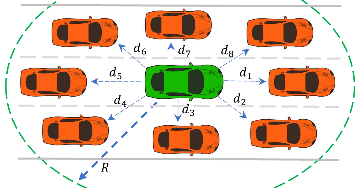
Figure 1: The distances between the AV (green vehicle) and each TV (red vehicles)

4.1.2 Action Space

The action space $\mathcal{A}$ includes the set of possible actions that the AV agent can take. Since the main goal is to avoid collisions by efficiently changing the lane, the action space includes three symbolic actions, called lane_keeping, left_lane_change, and right_lane_change which are converted to [0, 1, 2] in the DRL neural network, respectively. Unlike Baheri et al. (2020) and Wang et al. (2019), we removed $v_{x}$ from the action space since we employed a rule-based longitudinal velocity scheme to produce the favorable acceleration, creating a smooth driving.

4.1.3 Reward Function

We make use of a pre-defined reward function to help DRL to find the optimal policy. Reward function exerts a big impact on the training of DRL policy. Before introducing the reward structure, let’s assume the agent moves from the state $s$ to the next state $s^{\prime}$ by taking action $a$ at a given time step. The reward function for the AV is defined as follows:

$$R(s,a,s^{\prime})=w_{lc}r_{lc}(s,a)+w_{v}r_{v}(s,a)+w_{c}r_{c}(s,a)+w_{out}r_{out}(s,a)$$ (2)

where $r_{lc}(s,a)$, $r_{v}(s,a)$, $r_{c}(s,a)$, and $r_{out}(s,a)$ are the lane-change reward, velocity reward, collision reward, and off-road reward, respectively, and $w_{lc}$, $w_{v}$, $w_{c}$, and $w_{out}$ are the correspondent weights. To take the safety of passengers into account, the smoothness of the AV’s path on the road should be high. Therefore, the AV should not change the lane except for necessary times. That is why we devised the following lane-change reward:

$$r_{l}(s,a)=\begin{cases}-1&\text{if AV changed the lane}\\ 0&\text{otherwise}\\ \end{cases}$$ (3)

To make the agent agile, we must consider a velocity reward. We devised a reward function for the AV’s velocity in order to drive in the lanes with maximum allowed speed. Since we control the velocity of the AV using the rule-based methods, the AV does not have any control over the velocity. However, it can change the lane to find the maximum allowed velocity. Generally, the velocity reward is equal to $v_{x}$ with a correspondent weight, as $r_{v}(s,a)=v_{x}$. To avoid collision, the collision reward is defined as follows:

$$r_{c}(s,a)=\begin{cases}-(1-0.8\frac{x}{X})&\text{if collision occured}\\ 0&\text{otherwise}\\ \end{cases}$$ (4)

where $x$ is the longitudinal position of the point where a collision happens and $X$ is the total road length. The AV must not drive out of the legal lanes of the highway. Thus, as same as the collision reward, the lane deviation penalty reward function is given by:

$$r_{out}(s,a)=\begin{cases}-(1-0.8\frac{x}{X})&\text{if AV drives off the road}\\ 0&\text{otherwise}\\ \end{cases}$$ (5)

We have considered the weights for each reward subfunction through trial and error. Considering their importance, we assigned 5, 0.01, 100, and 100 to $w_{lc}$, $w_{v}$, $w_{c}$, and $w_{out}$, respectively.

After defining the environment components, we can define the governing rules for the highway driving to generate $\mathcal{A}^{safe}_{t}$, as presented in the following subsection.

4.2 SLP for AD

In order to extract $\mathcal{A}^{safe}_{t}$ for the AV in each step, an SLP uses all important information of the AV and TVs which received by the installed radar on the AV. We employ Prolog (Körner et al., 2022), as a symbolic logical programming language to define the desired safety rules in a highway environment. The useful data are vehicles’ IDs, lanes, dimensions, as well as longitudinal and lateral positions and velocities. Vehicles’ data is saved in each step and sent to the SLP core with the following fact clause:

$\verb|vehicle(ID,Lane,(P|_{x}\verb|,P|_{y}\verb|),(W,H),(V|_{x}\verb|,V|_{y}\verb|)).|$

where ID shows the identity code of a given vehicle, Lane is the vehicle lane, $\verb|(P|_{x}\verb|,P|_{y}\verb|)|$ are the logitudinal and lateral positions, $\verb|(V|_{x}\verb|,V|_{y}\verb|)|$ are the longitudinal and lateral velocities, and (W,H) are the length and width of the vehicle, respectively.

Afterward, we utilize human BK to shield unsafe actions from $\mathcal{A}$. Finding the target vehicles using the installed radar on the AV, the ralative positions of the TVs respect to the AV are described using their distance and the lanes. To do so, we divide the area around the AV to eight distinct sections; front, front_right, right, back_right, back, back_left, left, and front_left. This will assist us in finding the relative positions of each target vehicle in respect to the AV location. Knowledge of the relative positions of each TV helps us to find the busy sections around the AV, thereby making the decision-making process straight-forward. As an example, let’s consider this rule, ”If there is a TV in front of the AV and it has a similar lane to the AV lane, then the front of the AV is busy (front_is_busy).” We can show this rule using the following rule clause:

$\verb|front_is_busy:-|$

$\verb| lane(ego,Lane|_{1}\verb|), position_x(ego,P|_{x}^{1}\verb|),|$

$\verb| target_vehicle(Car), lane(Car,Lane|_{2}\verb|), position_x(Car,P|_{x}^{2}\verb|),|$

$\verb| Lane|_{1}\verb| is Lane|_{2}\verb|, direction(ego,Dir), distance(ego,Car,D), D>0,|$

$\verb| (Dir=right_to_left, P|_{x}^{2}\verb|<P|_{x}^{1}\verb|; Dir=left_to_right, P|_{x}^{2}\verb|>P|_{x}^{1}\verb|).|$

where ego and Car represent the AV’s and front TV’s ID, $\verb|Lane|_{1}$ and $\verb|Lane|_{2}$ indicate their lanes, and $\verb|P|_{x}^{1}$ and $\verb|P|_{x}^{2}$ indicate their longitudinal positions, respectively. Predicate target_vehicle(Car) identifies the TVs using the euclidean distance from the AV, and the AV identifies the front TV using the relative longitudinal position in each direction. Thus, front_is_busy is a predicate with boolean values to show when the front of the AV is busy. If a location is busy, then it is not free, as indicated in front_is_free:- not(front_is_busy). Similarly, we repeat the procedure for the rest of the sections around the AV to find the busy ones. When the AV knows about the busy and free sections, it can change the lane to the free lanes and avoid busy ones.

In the next step, a set of logical rules is applied to determine $\mathcal{A}^{safe}_{t}$. For example, the rule ”if there is no vehicle in the left sections, either keep your lane with a safe velocity or go to the left one,” or ”if the right and left sections are busy, then keep the lane” can be used to extract $\mathcal{A}^{safe}_{t}$ for lane changes. To implement the safety module, we have written an FOL program that consists of a set of rules that encode safety constraints. The following rule encodes the constraint that left_lane_change is safe only if going to the left section is valid (left_is_valid) and is safe (left_is_safe) at the same time, as shown in the following rule:

safe_actions(Action):-left_is_valid, left_is_safe, Action=left_lane_change.The predicate left_is_valid is unified with one if and only if the AV does not drive off the road by choosing the left_lane_change action. Likewise, the left_is_safe predicate is true when there is no TV in the left sections and the AV does not involve in collisions by taking the left_lane_change action. Similarly, if there is no vehicle in the right side of the AV (right_is_safe) and the right sections are valid (right_is_valid), then the right_lane_change action is safe, as shown in the following rule:

safe_actions(Action):-right_is_valid, right_is_safe, Action=right_lane_change.Furthermore, lane_keeping is always available for the autonomous vehicle to take. Since we design a velocity control scheme for the autonomous vehicle using an SLP in the next sections, the AV can take lane_keeping in each state and ensure avoiding collision with the front vehicle.

After generating all required rules, if the predicate safe_actions/1 succeeds, it means that the taken action is safe, and the Action variable is unified with the corresponding action. The safe_actions predicate returns each $a^{safe}_{t}$ seperately, but in order to find $\mathcal{A}^{safe}_{t}$, we need to backtrack (Ciatto et al., 2021) all individual safety rules and save their outputs to a list. This process can be performed using a built-in predicate named findall/3 which takes three arguments, including the Action variable, the safe_actions functor, and an orbitrary list name like Actions. Using the input arguments, this predicate will find all of the safe actions individually and save them to the Actions list.

4.3 DRLSL for AD

As shown in Fig. 2, once $\mathcal{A}^{safe}_{t}$ is determined using the FOL-based rules in the SLP core, we use PySwip library, as an interface between Prolog and Python, to connect the SLP core to the DRL agent. Thus, $\mathcal{A}^{safe}_{t}$ is passed to the DQN network as the available actions for the current state. When DQN agent employs symbolic logics (DQNSL), it chooses the best action from $\mathcal{A}^{safe}_{t}$ based on the $\epsilon$-greedy method, as shown in Algorithm 1. By restricting the entire action space to the $\mathcal{A}^{safe}_{t}$, we ensure that the DQN network learns only the safe actions and comply with the safety rules.

Integrating the SLP into DRL can lead to DRLSL, which considers safety constraints in addition to the policy of maximizing reward. The advantages of this approach include the ability to extract safe actions, which can reduce the risk of accidents and increase the reliability of the AD system. An SLP can also provide a transparent and interpretable framework for reasoning about safety, making it easier to verify and certify the system.

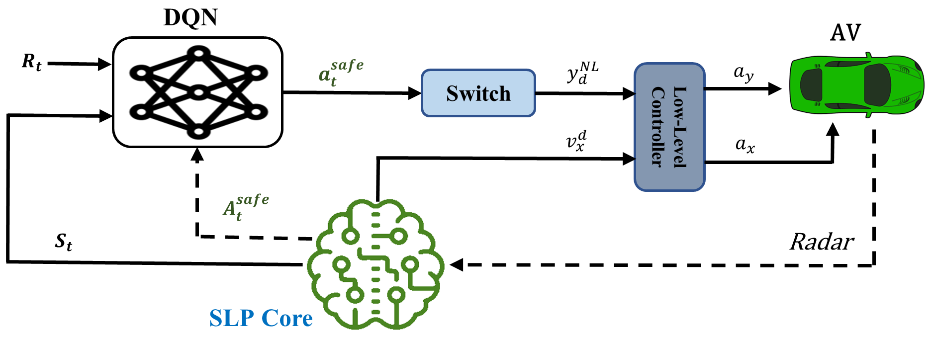
Figure 2: DQNSL using a SLP

It is worth noting that after finding $\mathcal{A}^{safe}_{t}$, DQNSL picks $a^{safe}_{t}$ from it. According to the taken action and the would-be lane, we find the lateral center of the next lane ($y^{NL}_{d}$). The process of finding the desired lateral center of each lane is performed using a Switch box, as indicated in Fig. 2. According to Fig. 3, for example, assume the AV is driving in the left-to-right direction and the middle lane (the fifth lane from top) and DQNSL commands to take the right_lane_change action. Thus, the sixth lane is the next lane, meaning that the $y^{NL}_{d}$ is $y^{6}_{d}$. Taking the $y^{6}_{d}$ as the desired output, a Proportional-Integral (PI) controller, as a low-level controller, produces a lateral acceleration $a_{y}$ to control the lateral position $y$ of the AV, as shown in Fig. 2.

5 Performance Evaluation

In this section, firstly, we describe the simulation settings and DRLSL agent’s network structure. Afterward, we discuss the longitudinal velocity control scheme. Finally, we elaborate upon the implementation of the proposed method and discuss the results.

5.1 Dataset

Numerous open-source platforms, including Carla (Dosovitskiy et al., 2017) and AirSim (Shah et al., 2018), exist to simulate traffic environments. However, it was difficult to implement simulated traffic based on actual data on these platforms. Our goal was to simulate a real-world agent by predicting drivers’ intentions, which made these platforms inappropriate. As a result, we created a Pygame-based traffic simulation environment (McGugan, 2007), as shown in Fig. 3.

Figure 3: Highway driving environment in Pygame (left-to-right direction). Green rectangle, red and white rectangles are AV, TVs, and other vehicles on the road, respectively.

Several studies (Ji et al., 2023; Chen et al., 2023; Tang et al., 2022) have examined highway driving by utilizing the NGSim (Yeo et al., 2008) and HighD (Krajewski et al., 2018) datasets. Both collections provide information regarding the lateral and longitudinal position, velocity, and acceleration of each vehicle on the road. The HighD dataset, in particular, is filmed using a drone camera that captures a 420-meter section of a German highway, offering accurate data even in situations where traffic is obstructed. The current research relies on the HighD dataset for both training and testing, using one of the most dense tracks for each stage of the study from a total of 60 tracks in the dataset, as depicted in Fig. 3. Although this method of studying traffic provides realistic results, it carries some limitations. Since we add a virtual AV to learn to drive efficiently among other vehicles, those vehicles are not aware the AV’s presence. In some situations, this leads to unavoidable accidents of whom the AV is not the cause. For example, when the AV is driving in a lane, another vehicle collides with it from back since the vehicle does not know the AV is on the road.

Accroding to the highD dataset, we assume an AV is driving on a two-directional, three-lane highway, as shown in Fig. 3. To clarify the position of each vehicle, we assign 1 to 6 to the highway lanes from top to buttom of Fig. 3. In the first three lanes, vehicles move in the right-to-left direction and in the rest, vehicles move in the left-to-right direction.

5.2 Network and Hyperparameters

Initially, we conducted assessments to identify hyperparameters that would ensure optimal and swift convergence. We determined the parameters after running preliminary tests. The network consisted of three fully connected layers, with the first two layers consisting of 256 nodes and the final layer consisting of three nodes to represent the action space. We employed the PyTorch library for neural network computations. Moreover, the ADAM algorithm, which is computationally efficient and rapidly converges, was used to optimize the networks. The discount factor was assigned a value of $\gamma=0.95$, while the learning rate was initially set as $\alpha_{i}=0.01$ and decays over each episode to reach the final value $\alpha_{e}=1e-4$. The experience replay memory $\mathcal{D}$ size is 100,000, and stochastic gradient descent batch size is 128. Except for the noisy networks, an epsilon-greedy exploration policy was implemented with a starting value of $\epsilon_{i}=0.1$ and decreasing to a minimum value of $\epsilon_{e}=0.001$. To stabilize the Q-network in the case of convergence, we updated the target network after 1,000 iterations. After describing the simulation settings, the defined reward function and the way we control $v_{x}$ to avoid collision with the front vehicle will be taken into account.

5.3 Longitudinal Velocity Control

In this section, we explain how the desired velocity of the AV is obtained in each state. We have written FOL-based rules for determining the longitudinal acceleration $a_{x}$ of the AV, which takes into account the current lane, maximum speed limit of the lane, the distance and speed of the front TV. The goals of the designed rules are collision avoidance with the front TV, making the driving smooth, as well as reducing the duration of driving along the track in the highway. The rules consider three scenarios; firstly, if there is no vehicle in front of the AV (front_is_free), then the desired velocity is set to the maximum speed limit of the current lane, reducing the time needed for moving along the highway and, at the same time, obeying the speed limit rules. Accordingly, $a_{x}$ is defined as following:

$$a_{x}=\frac{v_{max}-v_{x,AV}}{\Delta t}$$ (6)

where $\Delta t$, $v_{max}$, and $v_{x,AV}$ are the time step, the maximum allowed velocity in a given lane and the current velocity of the AV, respectively. As the second scenario, if there is a vehicle in front of the AV (front_is_busy), the desired velocity is calculated based on the distance and speed of that vehicle. In this case, we use the critical distance and actual distance to calculate the acceleration of the AV. If the distance is greater than the critical distance, $a_{x}$ is calculated using the following equation.

$$a_{x}=\frac{v^{2}_{x,TV}-v^{2}_{x,AV}}{2(D-C)}$$ (7)

where $v_{x,TV}$ is the longitudinal velocity of the front TV. Also, $D$ and $C$ are the actual distance and the critical distance between the AV and the TV. Here, we assume that $D$ is bigger than $C$. As the third scenario, when $D$ is lower than $C$, the AV must decelerate to avoid collision with the front TV, as shown in the following equation.

$$a_{x}=\frac{-v^{2}_{x,AV}}{2D}$$ (8)

After obtaining the desired acceleration, we update the desired velocity of the AV using $v_{x}^{d}=v_{x}+a_{x}\Delta t$ and after validating the velocity magnitude, it will be sent to a low-level controller, as shown in Fig. 2. Indeed, if the calculated velocity is greater than the maximum speed limit of the lane, the desired velocity is set to the maximum speed limit. Therefore, we make sure the AV follows the speed limit rule. Using a PI controller, as a low-level controller, helps to produce a continious and smooth $a_{x}$ and avoid collision with the front vehicle.

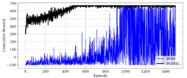
Figure 4: cumulative reward received by agents in each episode

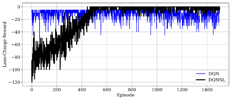
Figure 5: Lane-change reward per episode

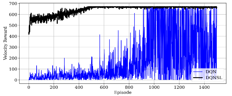
Figure 6: Velocity rewards received by agents

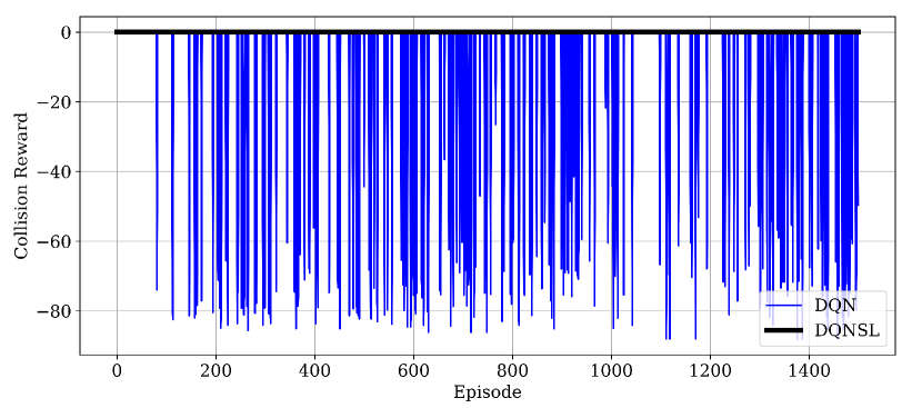
Figure 7: Collision rewards received by agents

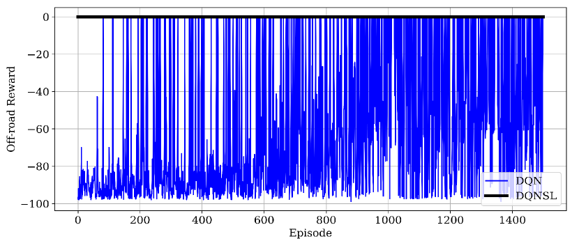
Figure 8: Off-road rewards received by agents

5.4 Results and Discussion

In this section, we present the results of our experiments using the proposed DQNSL approach. The experiments are divided to two main parts; training and test. Firstly, we evaluate the performance of the proposed method and compare the results of the DQNSL with those of DQN. We discuss the convergence of the reward function and the comparison of rewards between our method and the standard DQN algorithm. Additionally, we analyze the implications of our approach in terms of safety, rule adherence, and training efficiency. Then, we test the extracted RL models in different scenarios and evaluate each model performance.

5.4.1 Training

We trained both methods for 1,500 episodes using similar parameters for the reward function and the DQN network. Taking the advantage of the volocity control scheme, each agent was tasked with driving along an 840-meter track to reach the end of each episode. If a collision occurred or the agent deviated from the legal lanes, the episode was terminated. The results, as shown in Fig. 8, reveal that the DQNSL agent learns efficiently, while the DQN agent’s learning is highly unstable. This instability can be attributed to the fact that the DQN agent selects actions randomly from the entire action space, whereas the DQNSL agent selects actions only from the safe action set.

Furthermore, the reward results have multiple implications, particularly in terms of safety and reliability. The DQNSL agent consistently receives bigger rewards, indicating that it avoids unsafe actions such as collisions, lane violations, and dangerous maneuvers. On the other hand, during the initial stages of training, the DQN agent incurs significant negative rewards due to frequent lane violations and collisions.

Another notable difference is the speed of training. As observed in Fig. 8, the reward for the DQNSL agent converges after 500 episodes, whereas the DQN agent’s reward converges in an unstable manner after 970 episodes. The removal of unsafe actions plays a crucial role in this disparity. By constraining the action space and eliminating dangerous actions, we create a more favorable environment for the agent to discover the optimal policy. Restricting the dimensions of the action space simplifies the process of finding the best policy.

As mentioned in earlier sections, the reward function comprises four subfunctions: collision, off-road, lane change, and velocity rewards. We will now delve into each subfunction, compare the results, and discuss their implications. Figure 8 demonstrates that the DQNSL agent receives no penalties for collisions, indicating its successful avoidance of such incidents. Conversely, the DQN agent incurs an average penalty of -10.65 per episode. A similar trend can be observed for the off-road reward, as shown in Fig. 8. The DQN agent receives an average penalty of -60.1, while the DQNSL agent incurs no penalties since it remains within the legal lanes.

The lane change reward and velocity reward are the most important components of the DQNSL agent’s reward function, as the other rewards remain consistently at zero. As depicted in Fig. 8 and Fig. 8, the lane change reward and velocity exhibit convergence similar to the overall reward function, reaching optimal values at the same episode milestones. At the beginning of the learning process, the DQNSL agent receives negative rewards for lane changes as it explores safe state-action pairs by changing lanes. However, it gradually learns to avoid frequent lane changes and maintains a smoother trajectory. While the lane change reward continues to increase throughout the learning episodes, its negative value remains larger than that of the DQN agent. Since the DQN agent terminates episodes more quickly than the DQNSL agent, it does not have sufficient opportunities to engage in long maneuvers or lane changes.

Similarly, the DQNSL agent optimizes the velocity reward and reaches the maximum threshold within a given episode, as observed in Fig. 8. The DQNSL agent’s ability to regulate velocity enables it to achieve higher rewards compared to the DQN agent. The DQN agent, terminating episodes earlier, does not have the chance to fine-tune its velocity and consistently receives lower rewards.

In summary, our results demonstrate that the DQNSL approach significantly enhances safety during the exploration phase. The DQNSL agent outperforms the traditional DQN agent by avoiding unsafe actions and converging more quickly. The filtering of unsafe actions using SLP ensures a higher level of safety and facilitates a faster learning process for AVs in complex environments.

5.4.2 Test

In the test scenario, we conducted 50 episodes with a track length similar to the training scenario. However, unlike the training scenario, the test scenario featured a varying number of vehicles on the highway in each episode. Additionally, we deliberately excluded the safety module during testing to ensure fair comparison of results. According to Table 1, the findings demonstrate that both agents successfully learned to drive within the legal lanes. However, the DQN agent exhibited a significantly higher lane change frequency, averaging 5 lane changes per episode, which poses safety risks for the passengers. In contrast, the DQNSL model limited lane changes to an average of 1 time per episode, prioritizing a smoother driving experience while avoiding unnecessary lane changes.

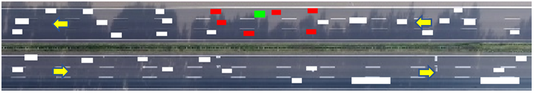
Figure 9: Right-to-left driving test scenario.

To compare the results of the velocity reward in the test scenarios, we assessed the performance of each agent by measuring the number of time steps required to reach the end of the track. A shorter time indicates a higher velocity reward. Table 1 shows that the DQNSL agent achieved this goal in 598 time steps on average, whereas the DQN agent required 670 time steps. Once again, the DQNSL agent outperformed the other agent, showcasing its efficiency in completing the task within a shorter duration.

We also examined the incidence of collisions across all episodes. As indicated in Table 1, the results revealed that the DQN agent collided with other vehicles on the road at a rate of 28%, while the collision rate for the DQNSL agent was reduced to 4%. It is worth noting that most of the collisions involving the DQNSL agent were unavoidable, as the other vehicles were unaware of the AV’s presence, thereby forcing it to take evasive maneuvers.

Table 1: Test results for 50 episodes

Direction	Left-to-Right		Right-to-Left
Agent	DQN	DQNSL	DQN	DQNSL
Lane changes	204	43	115	38
Collisions	14	2	5	3
Off road	0	0	33	0
Time step	657	592	684	603

Furthermore, we assessed the performance of both models when the autonomous vehicle traveled in the right-to-left direction, as shown in Fig. 9, in order to evaluate the generalizability of the defined rules on the highway. According to Table 1, the DQN agent struggled in this scenario, frequently veering out of the highway. In contrast, the DQNSL agent consistently remained within the confines of the highway, highlighting the effectiveness of the symbolic rules defined in the SLP core. The symbolic nature of these rules allows for easy generalization to new environments, enabling the seamless transfer and utilization of the defined rules in similar environments, ensuring broader applicability.

In summary, we have improved the safety of the DQN agent during the exploitation phase as well by eliminating dangerous actions from the set of possible actions during this phase. This enhancement brings DRL algorithms closer to the realities of AD systems. Moreover, we have shown that our method is able to perform well in the right-to-left driving scenario, indicating the generalizability of the symbolic rules which improves the transferability of the model to the new environments.

6 conclusion

In conclusion, this article proposed a novel approach for model-free deep reinforcement learning with symbolic logics (DRLSL) for safe autonomous driving. The main contribution of this approach is to ensure safety during the exploration phase of DRL by filtering out unsafe actions from the action set in a given state. The proposed method was evaluated on the HighD dataset, and the results showed a significant improvement in the safety level of the DRL algorithm. We trained the autonomous vehicle agent without any collisions, assisting the DRL agents to come to reality when training. Moreover, we significantly improved the stability and convergence speed of DRL during training. The result of the test scenarios indicated that our method is capable of driving with far less collision rates and lane violations. Moreover, in contrast to DRL only, DRLSL was able to drive in other side of the highway, placing emphasis on the generalizability of our algorithm. This approach has great potential to enhance the safety of autonomous driving systems, and it can be extended to other domains of DRL where safety is a critical concern.

References

- Achiam et al. (2017) Joshua Achiam, David Held, Aviv Tamar, and Pieter Abbeel. Constrained policy optimization. In International conference on machine learning, pp. 22–31. PMLR, 2017.
- Alshiekh et al. (2018) Mohammed Alshiekh, Roderick Bloem, Rüdiger Ehlers, Bettina Könighofer, Scott Niekum, and Ufuk Topcu. Safe reinforcement learning via shielding. In Proceedings of the AAAI Conference on Artificial Intelligence, volume 32, 2018.
- Baheri et al. (2020) Ali Baheri, Subramanya Nageshrao, H Eric Tseng, Ilya Kolmanovsky, Anouck Girard, and Dimitar Filev. Deep reinforcement learning with enhanced safety for autonomous highway driving. In 2020 IEEE Intelligent Vehicles Symposium (IV), pp. 1550–1555. IEEE, 2020.
- Belle (2020) Vaishak Belle. Symbolic logic meets machine learning: A brief survey in infinite domains. In Scalable Uncertainty Management: 14th International Conference, SUM 2020, Bozen-Bolzano, Italy, September 23–25, 2020, Proceedings 14, pp. 3–16. Springer, 2020.
- Calegari et al. (2020) Roberta Calegari, Giovanni Ciatto, Enrico Denti, and Andrea Omicini. Logic-based technologies for intelligent systems: State of the art and perspectives. Information, 11(3):167, 2020.
- Camacho et al. (2019) Alberto Camacho, Rodrigo Toro Icarte, Toryn Q Klassen, Richard Anthony Valenzano, and Sheila A McIlraith. Ltl and beyond: Formal languages for reward function specification in reinforcement learning. In IJCAI, volume 19, pp. 6065–6073, 2019.
- Chen et al. (2023) Jing Chen, Cong Zhao, Shengchuan Jiang, Xinyuan Zhang, Zhongxin Li, and Yuchuan Du. Safe, efficient, and comfortable autonomous driving based on cooperative vehicle infrastructure system. International journal of environmental research and public health, 20(1):893, 2023.
- Ciatto et al. (2021) Giovanni Ciatto, Roberta Calegari, and Andrea Omicini. Lazy stream manipulation in prolog via backtracking: The case of 2p-kt. In Logics in Artificial Intelligence: 17th European Conference, JELIA 2021, Virtual Event, May 17–20, 2021, Proceedings, pp. 407–420. Springer, 2021.
- Cropper & Dumančić (2022) Andrew Cropper and Sebastijan Dumančić. Inductive logic programming at 30: a new introduction. Journal of Artificial Intelligence Research, 74:765–850, 2022.
- De Giacomo et al. (2019) Giuseppe De Giacomo, Luca Iocchi, Marco Favorito, and Fabio Patrizi. Foundations for restraining bolts: Reinforcement learning with ltlf/ldlf restraining specifications. In Proceedings of the international conference on automated planning and scheduling, volume 29, pp. 128–136, 2019.
- De Raedt et al. (2019) Luc De Raedt, Robin Manhaeve, Sebastijan Dumancic, Thomas Demeester, and Angelika Kimmig. Neuro-symbolic= neural+ logical+ probabilistic. In NeSy’19@ IJCAI, the 14th International Workshop on Neural-Symbolic Learning and Reasoning, 2019.
- den Hengst et al. (2022) Floris den Hengst, Vincent François-Lavet, Mark Hoogendoorn, and Frank van Harmelen. Planning for potential: efficient safe reinforcement learning. Machine Learning, 111(6):2255–2274, 2022.
- Dong et al. (2019) Honghua Dong, Jiayuan Mao, Tian Lin, Chong Wang, Lihong Li, and Denny Zhou. Neural logic machines. arXiv preprint arXiv:1904.11694, 2019.
- Dosovitskiy et al. (2017) Alexey Dosovitskiy, German Ros, Felipe Codevilla, Antonio Lopez, and Vladlen Koltun. Carla: An open urban driving simulator. In Conference on robot learning, pp. 1–16. PMLR, 2017.
- Garcıa & Fernández (2015) Javier Garcıa and Fernando Fernández. A comprehensive survey on safe reinforcement learning. Journal of Machine Learning Research, 16(1):1437–1480, 2015.
- Gaur et al. (2022) Manas Gaur, Kalpa Gunaratna, Shreyansh Bhatt, and Amit Sheth. Knowledge-infused learning: A sweet spot in neuro-symbolic ai. IEEE Internet Computing, 26(4):5–11, 2022.
- Gu et al. (2022) Shangding Gu, Long Yang, Yali Du, Guang Chen, Florian Walter, Jun Wang, Yaodong Yang, and Alois Knoll. A review of safe reinforcement learning: Methods, theory and applications. arXiv preprint arXiv:2205.10330, 2022.
- Hasanbeig et al. (2019) Mohammadhosein Hasanbeig, Yiannis Kantaros, Alessandro Abate, Daniel Kroening, George J Pappas, and Insup Lee. Reinforcement learning for temporal logic control synthesis with probabilistic satisfaction guarantees. In 2019 IEEE 58th conference on decision and control (CDC), pp. 5338–5343. IEEE, 2019.
- Hazra & De Raedt (2023) Rishi Hazra and Luc De Raedt. Deep explainable relational reinforcement learning: A neuro-symbolic approach. arXiv preprint arXiv:2304.08349, 2023.
- Jansen et al. (2020) Nils Jansen, Bettina Könighofer, JSL Junges, AC Serban, and Roderick Bloem. Safe reinforcement learning using probabilistic shields. 2020.
- Ji et al. (2023) Kyoungtae Ji, Nan Li, Matko Orsag, and Kyoungseok Han. Hierarchical and game-theoretic decision-making for connected and automated vehicles in overtaking scenarios. Transportation research part C: emerging technologies, 150:104109, 2023.
- Jiang et al. (2021) Yuqian Jiang, Suda Bharadwaj, Bo Wu, Rishi Shah, Ufuk Topcu, and Peter Stone. Temporal-logic-based reward shaping for continuing reinforcement learning tasks. In Proceedings of the AAAI Conference on Artificial Intelligence, volume 35, pp. 7995–8003, 2021.
- Kimura et al. (2021a) Daiki Kimura, Subhajit Chaudhury, Akifumi Wachi, Ryosuke Kohita, Asim Munawar, Michiaki Tatsubori, and Alexander Gray. Reinforcement learning with external knowledge by using logical neural networks. arXiv preprint arXiv:2103.02363, 2021a.
- Kimura et al. (2021b) Daiki Kimura, Masaki Ono, Subhajit Chaudhury, Ryosuke Kohita, Akifumi Wachi, Don Joven Agravante, Michiaki Tatsubori, Asim Munawar, and Alexander Gray. Neuro-symbolic reinforcement learning with first-order logic. arXiv preprint arXiv:2110.10963, 2021b.
- Kiran et al. (2021) B Ravi Kiran, Ibrahim Sobh, Victor Talpaert, Patrick Mannion, Ahmad A Al Sallab, Senthil Yogamani, and Patrick Pérez. Deep reinforcement learning for autonomous driving: A survey. IEEE Transactions on Intelligent Transportation Systems, 23(6):4909–4926, 2021.
- Körner et al. (2022) Philipp Körner, Michael Leuschel, Joao Barbosa, Vitor Santos Costa, Verónica Dahl, Manuel V Hermenegildo, Jose F Morales, Jan Wielemaker, Daniel Diaz, Salvador Abreu, et al. Fifty years of prolog and beyond. Theory and Practice of Logic Programming, 22(6):776–858, 2022.
- Krajewski et al. (2018) Robert Krajewski, Julian Bock, Laurent Kloeker, and Lutz Eckstein. The highd dataset: A drone dataset of naturalistic vehicle trajectories on german highways for validation of highly automated driving systems. In 2018 21st International Conference on Intelligent Transportation Systems (ITSC), pp. 2118–2125. IEEE, 2018.
- Lillicrap et al. (2020) Timothy P Lillicrap, Adam Santoro, Luke Marris, Colin J Akerman, and Geoffrey Hinton. Backpropagation and the brain. Nature Reviews Neuroscience, 21(6):335–346, 2020.
- McGugan (2007) Will McGugan. Beginning game development with Python and Pygame: from novice to professional. Apress, 2007.
- Memarian et al. (2021) Farzan Memarian, Wonjoon Goo, Rudolf Lioutikov, Scott Niekum, and Ufuk Topcu. Self-supervised online reward shaping in sparse-reward environments. In 2021 IEEE/RSJ International Conference on Intelligent Robots and Systems (IROS), pp. 2369–2375. IEEE, 2021.
- Pham et al. (2018) Tu-Hoa Pham, Giovanni De Magistris, and Ryuki Tachibana. Optlayer-practical constrained optimization for deep reinforcement learning in the real world. In 2018 IEEE International Conference on Robotics and Automation (ICRA), pp. 6236–6243. IEEE, 2018.
- Riegel et al. (2020) Ryan Riegel, Alexander Gray, Francois Luus, Naweed Khan, Ndivhuwo Makondo, Ismail Yunus Akhalwaya, Haifeng Qian, Ronald Fagin, Francisco Barahona, Udit Sharma, et al. Logical neural networks. arXiv preprint arXiv:2006.13155, 2020.
- Sarker et al. (2021) Md Kamruzzaman Sarker, Lu Zhou, Aaron Eberhart, and Pascal Hitzler. Neuro-symbolic artificial intelligence. AI Communications, 34(3):197–209, 2021.
- Shah et al. (2018) Shital Shah, Debadeepta Dey, Chris Lovett, and Ashish Kapoor. Airsim: High-fidelity visual and physical simulation for autonomous vehicles. In Field and Service Robotics: Results of the 11th International Conference, pp. 621–635. Springer, 2018.
- Sutton & Barto (2018) Richard S Sutton and Andrew G Barto. Reinforcement learning: An introduction. MIT press, 2018.
- Tang et al. (2022) Xiaolin Tang, Kai Yang, Hong Wang, Jiahang Wu, Yechen Qin, Wenhao Yu, and Dongpu Cao. Prediction-uncertainty-aware decision-making for autonomous vehicles. IEEE Transactions on Intelligent Vehicles, 7(4):849–862, 2022.
- Tessler et al. (2018) Chen Tessler, Daniel J Mankowitz, and Shie Mannor. Reward constrained policy optimization. arXiv preprint arXiv:1805.11074, 2018.
- Wang et al. (2019) Junjie Wang, Qichao Zhang, Dongbin Zhao, and Yaran Chen. Lane change decision-making through deep reinforcement learning with rule-based constraints. In 2019 International Joint Conference on Neural Networks (IJCNN), pp. 1–6. IEEE, 2019.
- Xu et al. (2018) Jingyi Xu, Zilu Zhang, Tal Friedman, Yitao Liang, and Guy Broeck. A semantic loss function for deep learning with symbolic knowledge. In International conference on machine learning, pp. 5502–5511. PMLR, 2018.
- Yang et al. (2023) Wen-Chi Yang, Giuseppe Marra, Gavin Rens, and Luc De Raedt. Safe reinforcement learning via probabilistic logic shields. arXiv preprint arXiv:2303.03226, 2023.
- Yeo et al. (2008) Hwasoo Yeo, Alexander Skabardonis, John Halkias, James Colyar, and Vassili Alexiadis. Oversaturated freeway flow algorithm for use in next generation simulation. Transportation Research Record, 2088(1):68–79, 2008.
- Yu et al. (2023) Chao Yu, Xuejing Zheng, Hankz Hankui Zhuo, Hai Wan, and Weilin Luo. Reinforcement learning with knowledge representation and reasoning: A brief survey. arXiv preprint arXiv:2304.12090, 2023.
- Yu et al. (2021) Dongran Yu, Bo Yang, Dayou Liu, Hui Wang, and Shirui Pan. Recent advances in neural-symbolic systems: A survey. arXiv e-prints, pp. arXiv–2111, 2021.
- Zhang et al. (2023) Zheng Zhang, Levent Yilmaz, and Bo Liu. A critical review of inductive logic programming techniques for explainable ai. IEEE Transactions on Neural Networks and Learning Systems, 2023.