A log-linear model for non-stationary time series of counts

Abstract

We propose a new model for nonstationary integer-valued time series which is particularly suitable for data with a strong trend. In contrast to popular Poisson-INGARCH models, but in line with classical GARCH models, we propose to pick the conditional distributions from nearly scale invariant families where the mean absolute value and the standard deviation are of the same order of magnitude. As an important prerequisite for applications in statistics, we prove absolute regularity of the count process with exponentially decaying coefficients.

2020 Mathematics Subject Classification: Primary 60J10; secondary .
Keywords and Phrases: absolute regularity, count process, log-linear model, mixing, nonstationary process.
Short title: Log-linear count processes. version:

1. Motivation and introduction of the model

We propose a new model for time series of counts which is particularly appropriate for modeling explosive processes. So far, the literature on models for integer-valued time series is dominated by processes where the distribution of the count variables conditioned on the past is taken from the family of Poisson distributions, and where the intensities themselves are random and depend on lagged values of the count and the intensity variables; see e.g. Chapter 4 in Weiss (2018). While most of the results on statistical inference for these models are restricted to stationary time series, most of real life count data exhibit strong seasonal patterns and trends, see Figure 1. These features have to be incorporated into the model as simple detrending and deseasonalization is not feasible due to the discrete structure of the data.

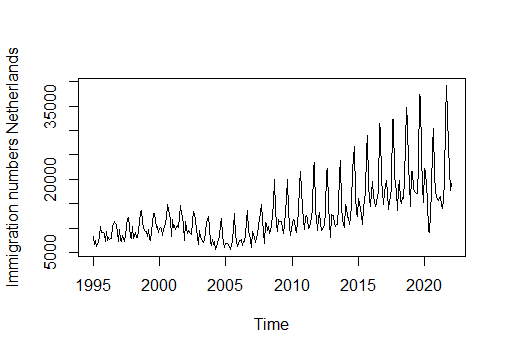
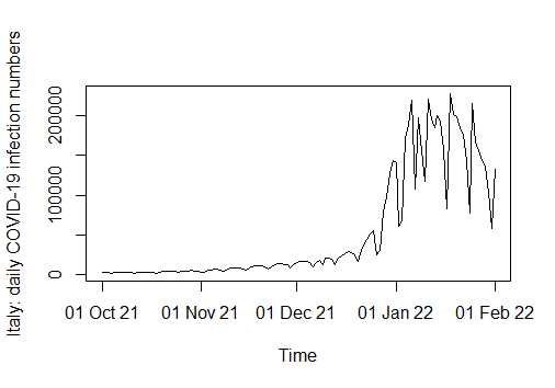
Figure 1. left: Monthly immigration numbers for the Netherlands with increasing trend and strongly increasing seasonality; right: daily COVID-19 infection numbers from Italy with explosive trend.

With a view towards a possible explosive behavior of processes to be modeled, we believe that it is natural that the expected values of the count variables are of the same order of magnitude as the respective standard deviations. This is in contrast to the family of Poisson distributions where, for $X\sim\mbox{Poi}(\sigma)$, $EX=\sigma$ but $\sqrt{\mathop{\rm var}\nolimits(X)}=\sqrt{\sigma}$, and so $\sqrt{\mathop{\rm var}\nolimits(X)}/EX$ tends to zero as $\sigma\to\infty$.

Note that overdispersion in the sense of $\mathop{\rm var}\nolimits(X_{t})=\eta EX_{t}$ for some $\eta>1$ can be incorporated in (log-)linear Poisson regression models by including exogeneous regressors, see e.g. Cameron and Trivedi (1986) and Xu et al. (2012). This approach is frequently used in various fields; e.g. in demography, health, and biology (as in Renshew and Haberman (2003), Powell et al. (2015), and Aagard, Lyons, and Thogmartin (2018)) and can be adapted to non-linear Poisson autoregressions: Suppose that

$$X_{t}\mid\sigma(\sigma_{0},X_{0},\ldots,\sigma_{t-1},X_{t-1})\,\sim\,\mbox{Poi}(\sigma_{t}\,Z_{t})\qquad\text{with }\quad\sigma_{t}\,=\,f(\sigma_{t-1},X_{t-1})$$

where $(Z_{t})_{t}$ is a sequence of i.i.d. random variables with mean $\mu_{z}$ and variance $\sigma_{z}^{2}\in(0,\infty)$ such that $Z_{t}$ is stochastically independent of $\sigma(\sigma_{0},X_{0},\ldots,\sigma_{t-1},X_{t-1})$. Then it follows from

$$E[X_{t}\mid\mathcal{\sigma}(\sigma_{0},X_{0},\ldots,\sigma_{t-1},X_{t-1})] = f(\sigma_{t-1},X_{t-1})\,\mu_{z}\quad\text{and}$$

$$\mathop{\rm var}\nolimits(X_{t}\mid\sigma(\sigma_{0},X_{0},\ldots,\sigma_{t-1},X_{t-1})) = f^{2}(\sigma_{t-1},X_{t-1})\,\sigma_{z}^{2}+f(\sigma_{t-1},X_{t-1})\,\mu_{z}.$$

that the degree of conditional dispersion can be changed adapting mean and variance of the exogenous regressors accordingly. Indeed, several well-known count time series models are special cases of these so-called mixed Poisson models. For instance, if the $Z_{t}$’s are binomial, then the conditional distribution of $X_{t}$ is a zero-inflated Poisson distribution and $Z_{t}$’s being Gamma distributed result in a negative binomial distributions, see e.g. Kremer et al. (2021) and Doukhan, Leucht, and Neumann (2022).

Here, we propose an alternative approach to assure that conditional expectation and variance of the same order of magnitude. We pick the conditional distributions from a family of (nearly) scale-invariant distributions. Candidates for such distributions can be found by discretizing scale-invariant continuous distributions. Let $Y$ be a non-negative random variable with a probability density $p$. Then we can define related integer-valued random variables $X_{\sigma}$ by setting

$$X_{\sigma}\,=\,\lfloor\sigma Y\rfloor,$$

i.e. $X_{\sigma}=k$ if and only if $\sigma Y\in[k,k+1)$. In what follows we denote the distribution of $X_{\sigma}$ by $P_{\sigma}$ and the corresponding probability mass function by $p_{\sigma}$. For example, if $Y$ is exponentially distributed with rate parameter $1$, then $\sigma Y$ is exponentially distributed with rate parameter $\sigma$ and $E[\sigma Y]=\sqrt{\mathop{\rm var}\nolimits(\sigma Y)}=\sigma$. We obtain for the corresponding integer-valued random variable $X_{\sigma}$ that

$$P_{\sigma}\big{(}\{k\}\big{)}\,=\,e^{-k/\sigma}\,-\,e^{-(k+1)/\sigma}\,=\,(1-p)^{k}\,p\qquad\forall k\in{\mathbb{N}}_{0},$$

where $p=1-e^{-1/\sigma}$. In this case, $X_{\sigma}$ has a geometric distribution with success parameter $p$. Furthermore, $EX_{\sigma}=(1-p)/p=e^{-1/\sigma}/(1-e^{-1/\sigma})$ and $\sqrt{\mathop{\rm var}\nolimits(X_{\sigma})}=\sqrt{(1-p)/p^{2}}=e^{-1/(2\sigma)}/(1-e^{-1/\sigma})$ are of the same order of magnitude as $\sigma\to\infty$. (This version of a geometric distribution has support ${\mathbb{N}}_{0}$ and describes the number of failures before the first success of independent Bernoulli trials with success parameter $p$.) Another example can be generated from the family of normal distributions. If $Y\sim N(0,\nu^{2})$, then $|Y|$ has a so-called half-normal distribution, and corresponding integer-valued random variables can be generated by setting $X_{\sigma}=\lfloor\sigma Y\rfloor$. In both cases, the families $(P_{\sigma})_{\sigma>0}$ satisfy the conditions imposed in this paper.

We impose a GARCH-type structure for the count process, i.e.

$$X_{t}\mid{\mathcal{F}}_{t-1}\,\sim\,P_{\sigma_{t}},$$ (1.1a)

where $${\mathcal{F}}_{s}=\sigma(\sigma_{0},X_{0},Z_{0},\ldots,\sigma_{s},X_{s},Z_{s}) \sigma_{t} \sigma_{t-1} X_{t-1} Z_{t-1} \sigma_{t}\,=\,f(\sigma_{t-1},X_{t-1})\,\cdot\,Z_{t-1}$$ and is a function of , , and an exogenous covariate which may describe e.g. seasonal effects or the effect of a changing environment. To be specific, we will assume that , which can be equivalently rewritten as

$$\ln(\sigma_{t})\,=\,\ln(f(\sigma_{t-1},X_{t-1}))\,+\,C_{t-1},$$ (1.1b)

where $C_{t}=\ln(Z_{t})$. To work with such processes it is necessary to have some probabilistic properties at our disposal. For classical GARCH processes, mixing properties have been known for a long time; see e.g. Boussama (1998) for linear and Carrasco and Chen (2002) and Francq and Zakoïan (2006) for nonlinear variants. These properties are typically stated for the bivariate process consisting of the observable and the state variables. In sharp contrast, for integer-valued GARCH, the state process $(\sigma_{t})_{t\in{\mathbb{N}}_{0}}$ is not mixing in general; see Remark 3 in Neumann (2011) for a counterexample. Moreover, mixing properties of classical GARCH processes can be deduced under weak moment conditions on the innovation distribution (see Francq and Zakoïan (2006)), while for Poisson-INGARCH time series all conditional moments given $\sigma_{t}$ exist. In contrast, here we require only $E[\ln^{+}(Y)]<\infty$ which means that only logarithmic conditional moments of the $X_{t}$ may exist.

In this paper we search for conditions that allow us to prove absolute regularity ($\beta$-mixing) of the count process $(X_{t})_{t\in{\mathbb{N}}_{0}}$. This will be done by a coupling approach described in greater detail in Section 2. To illustrate the usefulness of this result we discuss an application in statistics in Section 3. The proof of the main result is contained in Section 4 and the proof of asymptotic normality of a least squares estimator of a trend parameter is postponed to Section 5. Proofs of a few technical results are collected in a final Section 6.

2. Absolute regularity of the count process

Let $(\Omega,{\mathcal{A}},P)$ be a probability space and ${\mathcal{A}}_{1}$, ${\mathcal{A}}_{2}$ be two sub-$\sigma$-algebras of ${\mathcal{A}}$. Then the coefficient of absolute regularity is defined as

$$\beta({\mathcal{A}}_{1},{\mathcal{A}}_{2})\,=\,E\big{[}\sup\{|P(B\mid{\mathcal{A}}_{1})\,-\,P(B)|\colon\;\;B\in{\mathcal{A}}_{2}\}\big{]}.$$

For a process ${\mathbf{X}}=(X_{t})_{t\in{\mathbb{N}}_{0}}$ on $(\Omega,{\mathcal{F}},P)$, the coefficients of absolute regularity at the point $k$ are defined as

$$\beta^{X}(k,n)\,=\,\beta\big{(}\sigma(X_{0},X_{1},\ldots,X_{k}),\sigma(X_{k+n},X_{k+n+1},\ldots)\big{)}$$

and the (global) coefficients of absolute regularity as

$$\beta^{X}(n)\,=\,\sup\{\beta^{X}(k,n)\colon\;\;k\in{\mathbb{N}}_{0}\}.$$

The intended approach to prove absolute regularity is inspired by the fact that one can construct, on a suitable probability space $(\widetilde{\Omega},\widetilde{{\mathcal{F}}},\widetilde{P})$ two versions of the process $(X_{t})_{t\in{\mathbb{N}}_{0}}$, $({\widetilde{X}}_{t})_{t\in{\mathbb{N}}_{0}}$ and $({\widetilde{X}}_{t}^{\prime})_{t\in{\mathbb{N}}_{0}}$, such that $({\widetilde{X}}_{0},\ldots,{\widetilde{X}}_{k})$ and $({\widetilde{X}}_{0}^{\prime},\ldots,{\widetilde{X}}_{k}^{\prime})$ are independent and

$$\beta^{X}(k,n)\,=\,\widetilde{P}\left({\widetilde{X}}_{k+n+r}\neq{\widetilde{X}}_{k+n+r}^{\prime}\mbox{ for some }r\geq 0\right).$$

Since such an optimal coupling seems to be out of reach in our context we confine ourselves to construct a “reasonably good” coupling. Actually, if $({\widetilde{X}}_{t})_{t\in{\mathbb{N}}_{0}}$ and $({\widetilde{X}}_{t}^{\prime})_{t\in{\mathbb{N}}_{0}}$ defined on a common probability space $(\widetilde{\Omega},\widetilde{{\mathcal{F}}},\widetilde{P})$ are any two versions of $(X_{t})_{t\in{\mathbb{N}}_{0}}$ such that $({\widetilde{X}}_{0},\ldots,{\widetilde{X}}_{k})$ and $({\widetilde{X}}_{0}^{\prime},\ldots,{\widetilde{X}}_{k}^{\prime})$ are independent, then

$$\beta^{X}(k,n)$$ (2.1)

$$\leq \widetilde{E}\Big{[}\sup_{C\in\sigma({\mathcal{C}})}\big{\{}\big{|}\widetilde{P}\left(({\widetilde{X}}_{k+n},{\widetilde{X}}_{k+n+1},\ldots)\in C\mid{\widetilde{X}}_{0},\ldots,{\widetilde{X}}_{k}\right)$$

$$\qquad\qquad\qquad\,-\,\widetilde{P}\left(({\widetilde{X}}_{k+n}^{\prime},{\widetilde{X}}_{k+n+1}^{\prime},\ldots)\in C\mid{\widetilde{X}}_{0}^{\prime},\ldots,{\widetilde{X}}_{k}^{\prime}\right)\big{|}\big{\}}\Big{]}\qquad$$

$$\leq \widetilde{P}\left({\widetilde{X}}_{k+n+r}\neq{\widetilde{X}}_{k+n+r}^{\prime}\quad\mbox{for some }r\in{\mathbb{N}}_{0}\right)$$

$$= \widetilde{P}\left({\widetilde{X}}_{k+n}\neq{\widetilde{X}}_{k+n}^{\prime}\right)$$

$${}\,+\,\sum_{r=1}^{\infty}\widetilde{P}\left({\widetilde{X}}_{k+n+r}\neq{\widetilde{X}}_{k+n+r}^{\prime},{\widetilde{X}}_{k+n+r-1}={\widetilde{X}}_{k+n+r-1}^{\prime},\ldots,{\widetilde{X}}_{k+n}={\widetilde{X}}_{k+n}^{\prime}\right).$$

(In the second line of this display, $\sigma({\mathcal{C}})$ denotes the $\sigma$-algebra generated by the cylinder sets.) We construct on a suitable probability space $(\widetilde{\Omega},\widetilde{{\mathcal{F}}},\widetilde{P})$ two versions $\big{(}({\widetilde{\sigma}}_{t},{\widetilde{X}}_{t},{\widetilde{C}}_{t})\big{)}_{t\in{\mathbb{N}}_{0}}$ and $\big{(}({\widetilde{\sigma}}_{t}^{\prime},{\widetilde{X}}_{t}^{\prime},{\widetilde{C}}_{t}^{\prime})\big{)}_{t\in{\mathbb{N}}_{0}}$ of the process $\big{(}(\sigma_{t},X_{t},C_{t})\big{)}_{t\in{\mathbb{N}}_{0}}$ such that

$$\widetilde{P}\big{(}{\widetilde{X}}_{t}={\widetilde{X}}_{t}^{\prime}\mid{\widetilde{\sigma}}_{t},{\widetilde{\sigma}}_{t}^{\prime}\big{)}\,=\,\sum_{k=0}^{\infty}P_{{\widetilde{\sigma}}_{t}}(\{k\})\wedge P_{{\widetilde{\sigma}}_{t}^{\prime}}(\{k\})\,=\,1\,-\,d_{TV}\big{(}P_{{\widetilde{\sigma}}_{t}},P_{{\widetilde{\sigma}}_{t}^{\prime}}\big{)}.$$

Furthermore, if the density $p$ of $Y$ is nonincreasing on $[0,\infty)$ or differentiable everywhere on $(0,\infty)$ and $\int_{0}^{\infty}x|p^{\prime}(X)|\,dx<\infty$, then Lemma 6.1 shows that

$$d_{TV}\big{(}P_{\sigma}\,,\,P_{\sigma^{\prime}}\big{)}\,=\,O\big{(}|\ln(\sigma)\,-\,\ln(\sigma^{\prime})|\big{)}.$$

Hence, it is important to have the evolution of the process $\big{(}|\ln({\widetilde{\sigma}}_{t})-\ln({\widetilde{\sigma}}_{t}^{\prime})|\big{)}_{t\in{\mathbb{N}}_{0}}$ under control. Since $E\big{|}\ln(\lfloor\sigma Y\rfloor+1)-\ln(\lfloor\sigma^{\prime}Y\rfloor+1)\big{|}\leq\gamma\,|\ln(\sigma)-\ln(\sigma^{\prime})|$ for

$$\gamma\,:=\,\int_{0}^{\infty}\sup\{p(y)\colon\,y\geq x\}\,dx$$

(see Lemma 6.3 below) we suppose that the link function $f$ in (1.1b) satisfies the following contractive condition.

$$\big{|}\ln\big{(}f(\sigma,x)\big{)}\,-\,\ln\big{(}f(\sigma^{\prime},x^{\prime})\big{)}\big{|}$$ (2.2a)

$$\leq a\,|\ln(\sigma)\,-\,\ln(\sigma^{\prime})|\,+\,b\,|\ln(x+1)\,-\,\ln(x^{\prime}+1)|\qquad\forall\sigma,\sigma^{\prime}>0,x,x^{\prime}\in{\mathbb{N}}_{0},\qquad$$

where $$a,b\geq 0 a+b\gamma<1 C_{t} {\mathcal{F}}_{t-1} X_{t}$$ and . Furthermore, we assume that is independent of and , and that

$$M\,:=\,\sup_{t}E|C_{t}\,-\,EC_{t}|\,<\,\infty.$$ (2.2b)

Note that this includes the specification proposed in Fokianos and Tjøstheim (2011), where

$$\ln(\sigma_{t})\,=\,a\,\ln(\sigma_{t-1})\,+\,b\,\ln(X_{t-1}+1)\,+\,d\qquad\forall t\in{\mathbb{N}},$$

where the count variable $X_{t}$ given the past had a Poisson distribution with random intensity $\sigma_{t}$, and $d$ was a constant. In that case, for appropriately chosen values of the parameters $a$ and $b$, there exists a stationary process with such a dynamics.

Lemmas 4.1, 4.2, and 6.1 allow us to prove the following main result of this contribution.

Theorem 2.1.

Suppose that (1.1a), (1.1b), (2.2a), and (2.2b) are fulfilled, and let $E|\ln(\sigma_{0})|+E\ln^{+}(Y)<\infty$. We assume that the density $p\colon[0,\infty)\rightarrow[0,\infty)$ of $Y$ is either

• monotonously non-decreasing
  or

• everywhere differentiable.

In the former case we set $\gamma=\Gamma=1$ and in the latter $\gamma=\int_{0}^{\infty}\sup\{p(y)\colon\,y\geq x\}\,dx$ and $\Gamma=\big{(}1+\int_{0}^{\infty}x\,|p^{\prime}(x)|\,dx\big{)}/2$.

Then the count process $(X_{t})_{t\in{\mathbb{N}}_{0}}$ is absolutely regular ($\beta$-mixing), and the corresponding coefficients satisfy

$$\beta^{X}(n)\,\leq\,(a+b\gamma)^{n}\,\frac{\Gamma}{1-a}\,\Big{\{}2\,E|\ln(\sigma_{0})|\,+\,\frac{2b\,(\|p\|_{\infty}+E\ln^{+}(Y))\,+\,2M}{1-a-b}\Big{\}}.$$

Theorem 2.1 can serve as a basis for various statistical applications. For instance, confidence sets and statistical tests can be developed relying on Rio’s (1995) CLT for triangular arrays of nonstationary random variables; see Section 3 for details.

Remark 1.

The monotonicity assumption on $p$ is satisfied for instance if $Y$ is exponentially distributed or if it is half-normal. If $Y$ has a chi-square distribution with at least 3 degrees of freedom, then the corresponding density $p_{k}$ is unimodal with a mode at $k-2$. However it is differentiable everywhere on $(0,\infty)$ and

$$\int_{0}^{\infty}x\,|p_{k}^{\prime}(x)|\,dx = \int_{0}^{k-2}x\,p_{k}^{\prime}(x)\,dx\;-\;\int_{k-2}^{\infty}x\,p_{k}^{\prime}(x)\,dx$$

$$= 2(k-2)p_{k}(k-2)\,-\,\int_{0}^{k-2}p_{k}(x)\,dx\,+\,\int_{k-2}^{\infty}p_{k}(x)\,dx\,\leq\,\infty.$$

Hence, our conditions on the distribution of $Y$ are satisfied. Another example is given by the family of Cauchy distributions. Such a distribution has a density $p(x)=\pi\gamma/((x-\mu)^{2}+\gamma^{2})$ on ${\mathbb{R}}$, where $\mu\in{\mathbb{R}}$ is the location and $\gamma>0$ the scale parameter. If $Z$ follows such a distribution we would call the distribution of $Y=|Z|$ to be half-Cauchy. Such a distribution does not have finite moments of order greater than or equal to one, however, $E\ln^{+}(Y)$ is finite. $Y$ has a density $p(x)=\pi\gamma/((x-\mu)^{2}+\gamma^{2})+\pi\gamma/((x+\mu)^{2}+\gamma^{2})$ which is not non-increasing on $[0,\infty)$ if $|\mu|$ is large, however, it is decreasing on $[|\mu|,\infty)$. Again, our conditions are satisfied by this family of distributions.

3. An application in statistics

Suppose that we observe the random variables $X_{0},\ldots,X_{n}$ which follow a log-linear model similar to that proposed in Fokianos and Tjøstheim (2011). However, we include an increasing intercept term which causes a strong trend. To be specific, we assume that

$$\ln(\sigma_{t})\,=\,a\,\ln(\sigma_{t-1})\,+\,b\,\ln(X_{t-1}+1)\,+\,c\,\ln(t),$$

where $a\geq 0$, $b,c>0$, and $a+b\gamma<1$. We also assume that

$$X_{t}\mid{\mathcal{F}}_{t-1}\,\stackrel{{\scriptstyle d}}{{=}}\,\lfloor\sigma_{t}Y\rfloor.$$

Under mild regularity conditions we obtain that

$$E\ln(X_{t}+1)\,=\,\frac{c}{1-a-b}\ln(t)\,+\,O(1);$$ (3.1)

see Section 5 below. Hence, the parameter $\theta:=c/(1-a-b)$ characterizes the trend in the data. To estimate it, we may fit the regression model

$$\ln(X_{t}+1)\,=\,\theta\,\ln(t)\,+\,\varepsilon_{t},\qquad t=1,\ldots,n.$$

The ordinary least squares estimator is given as

$$\widehat{\theta}_{n}\,=\,\frac{\sum_{t=1}^{n}\ln(t)\,\ln(X_{t}+1)}{\sum_{t=1}^{n}\big{(}\ln(t)\big{)}^{2}}$$

and it is centered about the best projection $\bar{\theta}$ which is given as

$$\bar{\theta}\,=\,\mbox{arg}\,\min\sum_{t=1}^{n}E\big{|}\ln(X_{t}+1)\,-\,\theta\,\ln(t)\big{|}^{2}\,=\,\frac{\sum_{t=1}^{n}\ln(t)\,E\ln(X_{t}+1)}{\sum_{t=1}^{n}\big{(}\ln(t)\big{)}^{2}}.$$

To illustrate the dynamics of these models and the behavior of the empirical version of $\bar{\theta}$ we simulated trajectories (black) of samples of size $n=500$ with parameters chosen as $a=b=0.1$ and $c=2$ which give $\theta=2.5$, see Figure 2. The distribution of $Y$ is chosen to be either exponential (left) half-normal (right). The blue and red curves are given by $t\mapsto t^{\theta}$ and $t\mapsto t^{\widehat{\theta}}$, respectively, and can be viewed as approximations to the mean function $EX_{t}$.

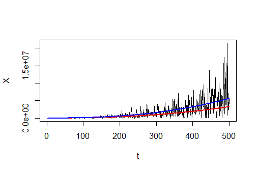
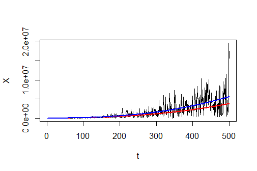
Figure 2. Simulated trajectories: left: $Y\sim Exp(1)$ ($\widehat{\theta}_{n}=2.41$), right: $Y\sim$ half-normal with $EY=1$ ($\widehat{\theta}=2.44$)

For the COVID-19 data from Italy, we estimate $\widehat{\theta}_{n}=2.48,$ see Figure 3.

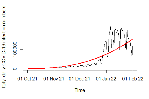
Figure 3. COVID-19 infection numbers with estimated trend curve.

Using the mixing property derived in Theorem 2.1 in conjunction with Rio’s (1995) central limit theorem for nonstationary and mixing random variables we can prove the following central limit theorem. In particular, it shows a non-standard rate of convergence of our estimator.

Proposition 3.1.

Suppose that the conditions of Theorem 2.1 are satisfied and

$$\ln(\sigma_{t})\,=\,a\,\ln(\sigma_{t-1})\,+\,b\,\ln(X_{t-1}+1)\,+\,c\,\ln(t),$$

where $a\geq 0$, $b,c>0$, and $a+b\gamma<1$. Moreover, assume that $\sigma_{0}\geq 1$ and $\|\ln(\sigma_{0})\|_{2+\delta}+\|\ln^{+}(Y)\|_{2+\delta}<\infty$ for some $\delta>0$. Then,

$$\sqrt{n}\,\ln(n)\,\big{(}\widehat{\theta}_{n}\,-\,\bar{\theta}\big{)}\,\stackrel{{\scriptstyle d}}{{\longrightarrow}}\,\mathcal{N}\left(0,\,\sigma^{2}\right),$$

where $\sigma^{2}=\mathop{\rm var}\nolimits\big{(}\ln(Y)\big{)}\,\Big{\{}\frac{b^{2}}{(1-(a+b))^{2}}\,+\,\frac{b}{a+b}\,\frac{1+(a+b)}{1-(a+b)}\Big{\}}$.

Remark 2.

Note that $\int_{0}^{1}|\ln(y)|^{2+\delta}p(y)\,dy<\infty$ if $\|p\|_{\infty}<\infty$, which implies that $E\big{[}|\ln(Y)|^{2+\delta}\big{]}\leq\|p\|_{\infty}\,\int_{0}^{1}|\ln(y)|^{2+\delta}\,dy+E\big{[}|\ln^{+}(Y)|^{2+\delta}\big{]}<\infty$. This means in particular that the variance of $\ln(Y)$ is finite under the above conditions.

4. Proof of Theorem 2.1

The proof of our main result is based on the following two lemmas.

Lemma 4.1.

Suppose that (1.1a), (1.1b), (2.2a), and (2.2b) are fulfilled, that the density $p$ of $Y$ is bounded, and let $E|\ln(\sigma_{0})|+E\ln^{+}(Y)<\infty$. Let $\big{(}({\widetilde{\sigma}}_{t},{\widetilde{X}}_{t},{\widetilde{C}}_{t})\big{)}_{t\in{\mathbb{N}}_{0}}$ and $\big{(}({\widetilde{\sigma}}_{t}^{\prime},{\widetilde{X}}_{t}^{\prime},{\widetilde{C}}_{t}^{\prime})\big{)}_{t\in{\mathbb{N}}_{0}}$ be independent versions of $\big{(}(\lambda_{t},X_{t},C_{t})\big{)}_{t\in{\mathbb{N}}_{0}}$ which are defined on a suitable probability space $\big{(}\widetilde{\Omega},\widetilde{{\mathcal{F}}},\widetilde{P}\big{)}$. Then

$$\sup_{k\in{\mathbb{N}}_{0}}\widetilde{E}\big{|}\ln({\widetilde{\sigma}}_{k})\,-\,\ln({\widetilde{\sigma}}_{k}^{\prime})\big{|}\,\leq\,2\,E|\ln(\sigma_{0})|\,+\,\frac{{2b\,(\|p\|_{\infty}+E\ln^{+}(Y))\,+\,2M}}{1-a-b}.$$

Proof.

It follows from (1.1b) and (2.2a) that

$$\big{|}\ln({\widetilde{\sigma}}_{t})\,-\,\ln({\widetilde{\sigma}}_{t}^{\prime})\big{|}$$

$$\leq a\,\big{|}\ln({\widetilde{\sigma}}_{t-1})\,-\,\ln({\widetilde{\sigma}}_{t-1}^{\prime})\big{|}\,+\,b\,\big{|}\ln({\widetilde{X}}_{t-1}+1)\,-\,\ln({\widetilde{X}}_{t-1}^{\prime}+1)\big{|}\,+\,\big{|}{\widetilde{C}}_{t-1}\,-\,{\widetilde{C}}_{t-1}^{\prime}\big{|}.$$

Note we obtain from Lemma 6.2 that $\widetilde{E}\big{(}|\ln({\widetilde{X}}_{t-1}+1)-\ln({\widetilde{\sigma}}_{t-1}+1)|\big{|}{\widetilde{\sigma}}_{t-1},{\widetilde{\sigma}}_{t-1}^{\prime}\big{)}=\widetilde{E}\big{(}|\ln({\widetilde{X}}_{t-1}+1)-\ln({\widetilde{\sigma}}_{t-1}+1)|\big{|}{\widetilde{\sigma}}_{t-1}\big{)}\leq\|p\|_{\infty}+E\ln^{+}(Y)$ and, analogously, $\widetilde{E}\big{(}|\ln({\widetilde{X}}_{t-1}^{\prime}+1)-\ln({\widetilde{\sigma}}_{t-1}^{\prime}+1)|\big{|}{\widetilde{\sigma}}_{t-1},{\widetilde{\sigma}}_{t-1}^{\prime}\big{)}\leq\|p\|_{\infty}+E\ln^{+}(Y)$. Therefore we obtain, for $t\geq 1$,

$$\widetilde{E}\Big{(}\big{|}\ln({\widetilde{\sigma}}_{t})\,-\,\ln({\widetilde{\sigma}}_{t}^{\prime})\big{|}\;\Big{|}\;{\widetilde{\sigma}}_{t-1},{\widetilde{\sigma}}_{t-1}^{\prime}\Big{)}$$

$$\leq a\,\big{|}\ln({\widetilde{\sigma}}_{t-1})\,-\,\ln({\widetilde{\sigma}}_{t-1}^{\prime})\big{|}\,+\,b\,\big{|}\ln({\widetilde{\sigma}}_{t-1}+1)\,-\,\ln({\widetilde{\sigma}}_{t-1}^{\prime}+1)\big{|}$$

$$\qquad+\,b\,\widetilde{E}\Big{(}\big{|}\ln({\widetilde{X}}_{t-1}+1)-\ln({\widetilde{\sigma}}_{t-1}+1)\big{|}\;\Big{|}\;{\widetilde{\sigma}}_{t-1},{\widetilde{\sigma}}_{t-1}^{\prime}\Big{)}$$

$$\qquad+\,b\,\widetilde{E}\Big{(}\big{|}\ln({\widetilde{X}}_{t-1}^{\prime}+1)-\ln({\widetilde{\sigma}}_{t-1}^{\prime}+1)\big{|}\;\Big{|}\;{\widetilde{\sigma}}_{t-1},{\widetilde{\sigma}}_{t-1}^{\prime}\Big{)}$$

$$\qquad+\,\widetilde{E}\Big{(}\big{|}{\widetilde{C}}_{t-1}\,-\,EC_{t-1}\big{|}\;\Big{|}\;{\widetilde{\sigma}}_{t-1},{\widetilde{\sigma}}_{t-1}^{\prime}\Big{)}\,+\,\widetilde{E}\Big{(}\big{|}{\widetilde{C}}_{t-1}^{\prime}\,-\,EC_{t-1}\big{|}\;\Big{|}\;{\widetilde{\sigma}}_{t-1},{\widetilde{\sigma}}_{t-1}^{\prime}\Big{)}$$

$$\leq (a+b)\,\big{|}\ln({\widetilde{\sigma}}_{t-1})\,-\,\ln({\widetilde{\sigma}}_{t-1}^{\prime})\big{|}\,+\,\bar{M},$$

where $\bar{M}=2b\,(\|p\|_{\infty}+E\ln^{+}(Y))+2M$. Taking expectation on both sides of this inequality we obtain that

$$\widetilde{E}\big{|}\ln({\widetilde{\sigma}}_{t})\,-\,\ln({\widetilde{\sigma}}_{t}^{\prime})\big{|}$$

$$\leq (a+b)\,\widetilde{E}\big{|}\ln({\widetilde{\sigma}}_{t-1})\,-\,\ln({\widetilde{\sigma}}_{t-1}^{\prime})\big{|}\;+\;\bar{M}$$

$$\leq (a+b)\,\Big{\{}(a+b)\,\widetilde{E}\big{|}\ln({\widetilde{\sigma}}_{t-2})\,-\,\ln({\widetilde{\sigma}}_{t-2}^{\prime})\big{|}\;+\;\bar{M}\Big{\}}\;+\;\bar{M}$$

$$\leq \,\ldots\,\leq\,(a+b)^{t}\;\widetilde{E}\big{|}\ln({\widetilde{\sigma}}_{0})\,-\,\ln({\widetilde{\sigma}}_{0}^{\prime})\big{|}\;+\;\bar{M}\,\big{\{}1\,+\,(a+b)\,+\,\cdots\,+\,(a+b)^{t-1}\big{\}}$$

$$\leq 2\,E|\ln(\sigma_{0})|\,+\,\frac{{\bar{M}}}{1-a-b}.$$

∎

Lemma 4.2.

Suppose that (1.1a), (2.2a), and (2.2b) are fulfilled, and let $E|\ln(\sigma_{0})|<\infty$. Furthermore, we assume that $p\colon[0,\infty)\rightarrow[0,\infty)$ is continuous and $\gamma:=\int_{0}^{\infty}\sup\{p(y)\colon\,y\geq x\}\,dx<\infty$.

Then there exist versions $\big{(}({\widetilde{\sigma}}_{t},{\widetilde{X}}_{t},{\widetilde{C}}_{t})\big{)}_{t\in{\mathbb{N}}_{0}}$ and $\big{(}({\widetilde{\sigma}}_{t}^{\prime},{\widetilde{X}}_{t}^{\prime},{\widetilde{C}}_{t-1}^{\prime})\big{)}_{t\in{\mathbb{N}}_{0}}$ of the process $\big{(}(\sigma_{t},X_{t},C_{t})\big{)}_{t\in{\mathbb{N}}_{0}}$ such that, for all $k,n\geq 0$,

(i) $$\quad\widetilde{E}\big{|}\ln({\widetilde{\sigma}}_{k+n})\,-\,\ln({\widetilde{\sigma}}_{k+n}^{\prime})\big{|}\,\leq\,(a+b\gamma)^{n}\,\widetilde{E}\big{|}\ln({\widetilde{\sigma}}_{k})\,-\,\ln({\widetilde{\sigma}}_{k}^{\prime})\big{|},$$

(ii) $$\quad\widetilde{E}\Big{[}\big{|}\ln({\widetilde{\sigma}}_{k+n+r})\,-\,\ln({\widetilde{\sigma}}_{k+n+r}^{\prime})\big{|}\,{\mathbbm{1}}\big{(}{\widetilde{X}}_{k+n}={\widetilde{X}}_{k+n}^{\prime},\ldots,{\widetilde{X}}_{k+n+r-1}={\widetilde{X}}_{k+n+r-1}^{\prime}\big{)}\Big{]}$$

$$\qquad\qquad\qquad\qquad\qquad\qquad\qquad\leq\,a^{r}\,(a+b\gamma)^{n}\,\widetilde{E}\big{|}\ln({\widetilde{\sigma}}_{k})\,-\,\ln({\widetilde{\sigma}}_{k}^{\prime})\big{|}\qquad\forall r\geq 1,$$

(iii) $$\quad\widetilde{P}\big{(}{\widetilde{X}}_{k+n+r}\neq{\widetilde{X}}_{k+n+r}^{\prime},{\widetilde{X}}_{k+n+r-1}={\widetilde{X}}_{k+n+r-1}^{\prime},\ldots,{\widetilde{X}}_{k+n}={\widetilde{X}}_{k+n}^{\prime}\big{)}$$

$$\qquad\leq\,\Gamma\,\widetilde{E}\Big{[}\big{|}\ln({\widetilde{\sigma}}_{k+n+r})\,-\,\ln({\widetilde{\sigma}}_{k+n+r}^{\prime})\big{|}\,{\mathbbm{1}}\big{(}{\widetilde{X}}_{k+n}={\widetilde{X}}_{k+n}^{\prime},\ldots,{\widetilde{X}}_{k+n+r-1}={\widetilde{X}}_{k+n+r-1}^{\prime}\big{)}\Big{]}\;\;\forall r\geq 0,$$

where $\Gamma=1$ if the density $p$ is non-increasing on $[0,\infty)$ and $\Gamma=\big{(}1+\int_{0}^{\infty}x|p^{\prime}(x)|\,dx\big{)}/2$ if $p$ is differentiable everywhere on $(0,\infty)$ with $\int_{0}^{\infty}x|p^{\prime}(x)|\,dx<\infty$.

Proof.

Let $t\geq k$. For given ${\widetilde{\sigma}}_{t}$ and ${\widetilde{\sigma}}_{t}^{\prime}$, we apply a maximal coupling of the respective random variables ${\widetilde{X}}_{t}$ and ${\widetilde{X}}_{t}^{\prime}$, i.e. ${\widetilde{X}}_{t}$ and ${\widetilde{X}}_{t}^{\prime}$ are defined such that

• $\widetilde{P}\big{(}{\widetilde{X}}_{t}=k\mid{\widetilde{\sigma}}_{t},{\widetilde{\sigma}}_{t}^{\prime}\big{)}\,=\,p_{{\widetilde{\sigma}}_{t}}(k)\quad\mbox{and}\quad\widetilde{P}\big{(}{\widetilde{X}}_{t}^{\prime}=k\mid{\widetilde{\sigma}}_{t},{\widetilde{\sigma}}_{t}^{\prime}\big{)}\,=\,p_{{\widetilde{\sigma}}_{t}^{\prime}}(k)\qquad\forall k\in{\mathbb{N}}_{0}$,

• $\widetilde{P}\big{(}{\widetilde{X}}_{t}={\widetilde{X}}_{t}^{\prime}\mid{\widetilde{\sigma}}_{t},{\widetilde{\sigma}}_{t}^{\prime}\big{)}\,=\,1\,-\,d_{TV}\big{(}P_{{\widetilde{\sigma}}_{t}},P_{{\widetilde{\sigma}}_{t}^{\prime}}\big{)}\,=\,\sum_{k=0}^{\infty}p_{{\widetilde{\sigma}}_{t}}(k)\wedge p_{{\widetilde{\sigma}}_{t}^{\prime}}(k)$.

(Note that our definition of the total variation norm differs from that in Lindvall (1992) by the factor 2.) Furthermore, and in contrast to the construction used for the proof of Theorem 5.2 in Lindvall (1992, Chapter I), we couple ${\widetilde{X}}_{t}$ and ${\widetilde{X}}_{t}^{\prime}$ such that ${\widetilde{X}}_{t}\geq{\widetilde{X}}_{t}^{\prime}$ holds with conditional probability 1 if ${\widetilde{\sigma}}_{t}\geq{\widetilde{\sigma}}_{t}^{\prime}$ and, vice versa, ${\widetilde{X}}_{t}\leq{\widetilde{X}}_{t}^{\prime}$ holds with conditional probability 1 if ${\widetilde{\sigma}}_{t}\leq{\widetilde{\sigma}}_{t}^{\prime}$. (This is possible since $\lfloor\sigma Y\rfloor$ is stochastically greater than $\lfloor\sigma^{\prime}Y\rfloor$ if $\sigma\geq\sigma^{\prime}$.) And finally, we choose the exogenous variables such that ${\widetilde{C}}_{t}={\widetilde{C}}_{t}^{\prime}$.

(i)  Let $k<t\leq k+n$. Since ${\widetilde{X}}_{t}-{\widetilde{X}}_{t}^{\prime}$ has the same sign as ${\widetilde{\sigma}}_{t}-{\widetilde{\sigma}}_{t}^{\prime}$, $\ln({\widetilde{X}}_{t}+1)-\ln({\widetilde{X}}_{t}^{\prime}+1)$ is either non-negative or non-positive with conditional probability 1, and we obtain by Lemma 6.3

$$\widetilde{E}\Big{(}\big{|}\ln({\widetilde{X}}_{t}+1)\,-\,\ln({\widetilde{X}}_{t}^{\prime}+1)\big{|}\;\Big{|}\;{\widetilde{\sigma}}_{t-1},{\widetilde{\sigma}}_{t-1}^{\prime}\Big{)} = \widetilde{E}\Big{|}\Big{(}\ln({\widetilde{\sigma}}_{t})\,-\,\ln({\widetilde{\sigma}}_{t}^{\prime})\;\Big{|}\;{\widetilde{\sigma}}_{t-1},{\widetilde{\sigma}}_{t-1}^{\prime}\Big{)}\Big{|}$$

$$\leq \gamma\,\big{|}\ln({\widetilde{\sigma}}_{t-1})\,-\,\ln({\widetilde{\sigma}}_{t-1}^{\prime})\big{|}.$$

This yields that

$$\widetilde{E}\Big{(}\big{|}\ln({\widetilde{\sigma}}_{t})\,-\,\ln({\widetilde{\sigma}}_{t}^{\prime})\big{|}\;\Big{|}\;{\widetilde{\sigma}}_{t-1},{\widetilde{\sigma}}_{t-1}^{\prime}\Big{)}\,\leq\,(a+b\gamma)\,\big{|}\ln({\widetilde{\sigma}}_{t-1})\,-\,\ln({\widetilde{\sigma}}_{t-1}^{\prime})\big{|}.$$

Taking expectation on both sides of this inequality, and using the resulting inequality $n$ times we obtain

$$\widetilde{E}\big{|}\ln({\widetilde{\sigma}}_{k+n})\,-\,\ln({\widetilde{\sigma}}_{k+n}^{\prime})\big{|}\,\leq\,(a+b\gamma)^{n}\,\widetilde{E}\big{|}\ln({\widetilde{\sigma}}_{k})\,-\,\ln({\widetilde{\sigma}}_{k}^{\prime})\big{|}.$$

(ii)  Let now $t=k+n+r>k+n$. Then we obtain immediately

$$\big{|}\ln({\widetilde{\sigma}}_{t})\,-\,\ln({\widetilde{\sigma}}_{t}^{\prime})\big{|}\,{\mathbbm{1}}\big{(}{\widetilde{X}}_{k+n}={\widetilde{X}}_{k+n}^{\prime},\ldots,{\widetilde{X}}_{t-1}={\widetilde{X}}_{t-1}^{\prime}\big{)}$$

$$\leq a\,\big{|}\ln({\widetilde{\sigma}}_{t-1})\,-\,\ln({\widetilde{\sigma}}_{t-1}^{\prime})\big{|}\,{\mathbbm{1}}\big{(}{\widetilde{X}}_{k+n}={\widetilde{X}}_{k+n}^{\prime},\ldots,{\widetilde{X}}_{t-2}={\widetilde{X}}_{t-2}^{\prime}\big{)}$$

$$\leq \cdots\,\leq\,a^{r}\,\big{|}\ln({\widetilde{\sigma}}_{k+n})\,-\,\ln({\widetilde{\sigma}}_{k+n}^{\prime})\big{|},$$

which yields (ii). Statement (iii) follows from Lemma 6.1. ∎

Now we are in a position to prove our main result.

Proof of Theorem 2.1.

Let $\big{(}({\widetilde{\sigma}}_{t},{\widetilde{X}}_{t},{\widetilde{C}}_{t})\big{)}_{t\in{\mathbb{N}}_{0}}$ and $\big{(}({\widetilde{\sigma}}_{t}^{\prime},{\widetilde{X}}_{t}^{\prime},{\widetilde{C}}_{t}^{\prime})\big{)}_{t\in{\mathbb{N}}_{0}}$ be two versions of the process $\big{(}(\sigma_{t},X_{t},C_{t})\big{)}_{t\in{\mathbb{N}}_{0}}$, where $({\widetilde{\sigma}}_{0},{\widetilde{X}}_{0},{\widetilde{C}}_{0},\ldots,{\widetilde{\sigma}}_{k-1},{\widetilde{X}}_{k-1},{\widetilde{C}}_{k-1},{\widetilde{\sigma}}_{k},{\widetilde{X}}_{k})$ and $({\widetilde{\sigma}}_{0}^{\prime},{\widetilde{X}}_{0}^{\prime},{\widetilde{C}}_{0}^{\prime},\ldots,{\widetilde{\sigma}}_{k-1}^{\prime},{\widetilde{X}}_{k-1}^{\prime},{\widetilde{C}}_{k-1}^{\prime},{\widetilde{\sigma}}_{k}^{\prime},{\widetilde{X}}_{k}^{\prime})$ are independent, and where ${\widetilde{C}}_{k},{\widetilde{\sigma}}_{k+1},{\widetilde{X}}_{k+1},{\widetilde{\sigma}}_{k+2},{\widetilde{X}}_{k+2},\ldots$ are coupled with their respective counterparts ${\widetilde{C}}_{k}^{\prime},{\widetilde{\sigma}}_{k+1}^{\prime},{\widetilde{X}}_{k+1}^{\prime},{\widetilde{\sigma}}_{k+2}^{\prime},{\widetilde{X}}_{k+2}^{\prime},\ldots$ as described in the proof of Lemma 4.2. Then we obtain from (2.1) and Lemmas 4.1 and 4.2 that

$$\beta^{X}(k,n)$$

$$\leq \widetilde{P}\left({\widetilde{X}}_{k+n}\neq{\widetilde{X}}_{k+n}^{\prime}\right)$$

$${}\,+\,\sum_{r=1}^{\infty}\widetilde{P}\left({\widetilde{X}}_{k+n+r}\neq{\widetilde{X}}_{k+n+r}^{\prime},{\widetilde{X}}_{k+n+r-1}={\widetilde{X}}_{k+n+r-1}^{\prime},\ldots,{\widetilde{X}}_{k+n}={\widetilde{X}}_{k+n}^{\prime}\right)$$

$$\leq \Gamma\,\sum_{r=0}^{\infty}a^{r}\,(a+b\gamma)^{n}\,\big{\{}2\,E\big{|}\ln(\sigma_{0})\big{|}\,+\,\frac{{2b\,(\|p\|_{\infty}+E\ln^{+}(Y))\,+\,2M}}{1-a-b}\big{\}}.$$

∎

5. Proof of Proposition 3.1

The following lemma is a consequence of a CLT in Rio (1995) and it serves as a basis for the proof of Proposition 3.1.

Lemma 5.1.

Suppose that $(X_{t,n})_{t=1,\dots n},\;n\in{\mathbb{N}},$ is a triangular array of centered random variables with $\sup_{t\leq n}(\|X_{t,n}\|_{2+\delta})=O(n^{-1/2})$ for some $\delta>0$, where $\|X_{t,n}\|_{q}:=(E|X_{t,n}|^{q})^{1/q}$. Further assume that the array is absolutely regular with exponentially decaying mixing coefficients $\beta_{(n)}(k)\leq\rho_{k}$ for some $\rho<1$. If additionally $V_{n,n}:=\mathop{\rm var}\nolimits(\sum_{t=1}^{n}X_{t,n})$ satisfies $\liminf_{n\to\infty}V_{n,n}>0$, then

$$\sum_{t=1}^{n}\frac{X_{t,n}}{V_{n,n}^{1/2}}\,\stackrel{{\scriptstyle d}}{{\longrightarrow}}\,Z\sim\mathcal{N}(0,1).$$

Proof of Lemma 5.1.

We apply Corollary 1 in Rio (1995). To this end, we validate conditions (a) and (b) therein. Assumption (a) reads

$$\limsup_{n\to\infty}\max_{i\leq n}\frac{\mathop{\rm var}\nolimits(\sum_{t=1}^{i}X_{t,n})}{V_{n,n}}\,<\,\infty.$$

In view of our assumption $\liminf_{n\to\infty}V_{n,n}>0$, it suffices to show that

$$\limsup_{n\in{\mathbb{N}}}\sum_{s,t=1}^{n}\left|\mathop{\rm cov}\nolimits({X_{s,n}}\,,\,{X_{t,n}})\right|\,\leq\,C.$$ (5.1)

Recall that the $\beta$-mixing coefficients serve as an upper bound for the $\alpha$-mixing coefficients. By the covariance inequality for $\alpha$-mixing random variables (see e.g. Doukhan (1994, Thm. 3, Sect. 1.2.2)) we obtain

$$\left|\mathop{\rm cov}\nolimits({X_{s,n}}\,,\,{X_{t,n}})\right|\,\leq\,8\,\alpha_{(n)}^{X}(|s-t|)^{(2+\delta)/\delta}\,\|X_{s,n}\|_{2+\delta}\,\|X_{t,n}\|_{2+\delta}$$

which then gives (5.1) under our moment conditions by the exponential decay of the strong mixing coefficients.

It remains to check (b) in Corollary 1 in Rio (1995), that is

$$\sum_{t=1}^{n}\int_{0}^{1}\,\alpha_{(n)}^{-1}\left(\frac{x}{2}\right)\,Q_{t,n}^{2}(x)\,\min\left\{1\,,\,\alpha_{(n)}^{-1}\left(\frac{x}{2}\right)\,Q_{t,n}(x)\,\right\}\,dx\mathop{\longrightarrow}\limits_{n\to\infty}0.$$ (5.2)

Here, $Q_{t,n}$ denotes the inverse of the survival function $z\mapsto P(|X_{t,n}|\,>\,z\,V_{n,n}^{1/2})$ and $\alpha_{(n)}^{-1}$ denotes the inverse of $z\mapsto\alpha(\lfloor z\rfloor)$. First, note that $\alpha_{(n)}^{-1}(x/2)\leq C_{1}-C_{2}\,\ln(x)$ for some $C_{1},\,C_{2}\in(0,\infty)$ in view of the exponential decay of the mixing coefficients. Second, we obtain by Markov’s inequality

$$P(|X_{t,n}|\,>\,z\,V_{n,n}^{1/2})\,\leq\,\frac{E|X_{t,n}|^{2+\delta}}{z^{2+\delta}\,V_{n,n}^{(2+\delta)/2}}$$

which leads to

$$Q_{t,n}(x)\leq x^{-1/(2+\delta)}\left(\frac{\|X_{t,n}\|_{2+\delta}}{V_{n,n}^{1/2}}\right).$$

From this, and using the rough estimate $\min\left\{1,\alpha_{(n)}^{-1}\left(\frac{x}{2}\right)Q_{t,n}(x)\right\}\leq\alpha_{(n)}^{-\delta/2}\left(\frac{x}{2}\right)Q_{t,n}^{\delta/2}(x)$, we can deduce that the r.h.s. of (5.2) can be bounded from above by

$$\widetilde{C}\,\int_{0}^{1}\,|\ln(x)|^{1+\delta/2}\,x^{-(2+\delta/2)/(2+\delta)}\,dx\,\cdot\,\sum_{t=1}^{n}\left(\frac{\|X_{t,n}\|_{2+\delta}}{V_{n,n}^{1/2}}\right)^{2+\delta/2}$$

which tends to zero as $\sup_{t\leq n}(\|X_{t,n}\|_{2+\delta})=O(n^{-1/2})$. ∎

Before we turn to the proof of Proposition 3.1 we derive a few useful approximations. Since $\sigma_{0}\geq 1$ and $\ln(\sigma_{t})\geq a\ln(\sigma_{t-1})\,+\,c\,\ln(t)$ we see inductively that under the conditions of Proposition 3.1

$$\sigma_{t}\,\geq\,t^{c}\qquad\forall t\geq 1.$$ (5.3)

In what follows we shall get rid of the cumbersome terms $\ln(X_{t}+1)$. Note that the vector $(X_{0},\ldots,X_{n})$ has the same distribution as $(\lfloor\sigma_{0}Y_{0}\rfloor,\ldots,\lfloor\sigma_{n}Y_{n}\rfloor)$, where $Y_{t}$ has the same distribution as $Y$ and is independent of $\sigma_{0},\ldots,\sigma_{t},Y_{0},\ldots,Y_{t-1}$. To simplify the representation we suppose that $X_{t}=\lfloor\sigma_{t}Y_{t}\rfloor$.

Since

$$\ln(\sigma_{t}Y_{t})\leq\ln(X_{t}+1)\leq\ln(\sigma_{t}Y_{t}+1)\leq\ln(\sigma_{t}(Y_{t}+1/t^{c}))$$

we obtain

$$\ln\big{(}X_{t}+1\big{)}\,-\,\ln\big{(}\sigma_{t}Y_{t}\big{)}\,\leq\,\ln\big{(}\sigma_{t}(Y_{t}+1/t^{c})\big{)}\,-\,\ln\big{(}\sigma_{t}Y_{t}\big{)}$$

and hence, for $\rho\leq 2+\delta$,

$$E\big{|}\ln\big{(}X_{t}+1\big{)}\,-\,\ln\big{(}\sigma_{t}Y_{t}\big{)}\big{|}^{\rho} \leq E\big{|}\ln\big{(}\sigma_{t}(Y_{t}+1/t^{c})\big{)}\,-\,\ln\big{(}\sigma_{t}Y_{t}\big{)}\big{|}^{\rho}$$ (5.4)

$$= E\big{|}\ln\big{(}(Y_{t}+1/t^{c})\big{)}\,-\,\ln\big{(}Y_{t}\big{)}\big{|}^{\rho}\mathop{\longrightarrow}\limits_{t\to\infty}0.\qquad$$

The above representation allows us to represent $\ln(\sigma_{t})$ in a suitable form:

$$\ln(\sigma_{t}) = (a+b)\,\ln(\sigma_{t-1})\,+\,b\,\ln(Y_{t-1})\,+\,b\,\big{[}\ln(X_{t-1}+1)-\ln(\sigma_{t-1}Y_{t-1})\big{]}\,+\,c\,\ln(t)$$ (5.5)

$$= (a+b)\,\Big{\{}(a+b)\,\ln(\sigma_{t-2})\,+\,b\,\ln(Y_{t-2})\,+\,b\,\big{[}\ln(X_{t-2}+1)-\ln(\sigma_{t-2}Y_{t-2})\big{]}\,+\,c\,\ln(t-1)\Big{\}}$$

$$\quad{}\,+\,b\,\ln(Y_{t-1})\,+\,b\,\big{[}\ln(X_{t-1}+1)-\ln(\sigma_{t-1}Y_{t-1})\big{]}\,+\,c\,\ln(t)$$

$$= \ldots\,=\,(a+b)^{t}\,\ln(\sigma_{0})$$

$$\qquad\,+\,b\,\sum_{s=1}^{t}(a+b)^{s-1}\,\ln(Y_{t-s})$$

$$\qquad\,+\,b\,\sum_{s=1}^{t}(a+b)^{s-1}\,\big{[}\ln(X_{t-s}+1)\,-\,\ln(\sigma_{t-s}Y_{t-s})\big{]}$$

$$\qquad\,+\,c\,\Big{\{}\sum_{s=0}^{t-1}(a+b)^{s}\,\ln(t-s)\,-\,\frac{1}{1-a-b}\,\ln(t)\Big{\}}$$

$$\qquad\,+\,\frac{c}{1-a-b}\,\ln(t).$$

The first four terms on the right-hand side are stochastically bounded, and the fifth one is dominating.

Now we are in a position to approximate the covariance structure of $\ln(X_{t}+1)$. Since it follows from (5.4) that $\big{\|}\ln(X_{t-s}+1)-\ln(\sigma_{t-s}Y_{t-s})\big{\|}_{2}\mathop{\longrightarrow}\limits_{t\to\infty}0$ we obtain by Minkowski’s inequality

$$\Big{\|}b\,\sum_{s=1}^{t}(a+b)^{s-1}\,\big{[}\ln(X_{t-s}+1)-\ln(\sigma_{t-s}Y_{t-s})\big{]}\Big{\|}_{2}\,\leq\,b\,\sum_{s=1}^{t}(a+b)^{s-1}\,\big{\|}\ln(X_{t-s}+1)-\ln(\sigma_{t-s}Y_{t-s})\big{\|}_{2}\mathop{\longrightarrow}\limits_{t\to\infty}0.$$

This means that the limits of the covariances arise from the terms in the fourth from last row in (5.5):

$$\mathop{\rm cov}\nolimits\big{(}\ln(\sigma_{t}),\ln(\sigma_{t-u})\big{)}\mathop{\longrightarrow}\limits_{t\to\infty}\mathop{\rm var}\nolimits(\ln(Y))\,b^{2}\,\frac{(a+b)^{u}}{1\,-\,(a+b)^{2}}.$$ (5.6)

This implies

$$\mathop{\rm var}\nolimits\big{(}\ln(X_{t}+1)\big{)} \mathop{\longrightarrow}\limits_{t\to\infty} \lim_{t\to\infty}\mathop{\rm var}\nolimits\big{(}\ln(\sigma_{t})+\ln(Y_{t})\big{)}$$ (5.7)

$$= \lim_{t\to\infty}\mathop{\rm var}\nolimits\big{(}\ln(\sigma_{t})\big{)}\quad+\quad\mathop{\rm var}\nolimits\big{(}\ln(Y)\big{)}$$

$$= \mathop{\rm var}\nolimits\big{(}\ln(Y)\big{)}\,\Big{\{}\frac{b^{2}}{1-(a+b)^{2}}\,+\,1\Big{\}}$$

and, for $u\geq 1$,

$$\mathop{\rm cov}\nolimits\big{(}\ln(X_{t}+1),\ln(X_{t-u}+1)\big{)} \mathop{\longrightarrow}\limits_{t\to\infty} \lim_{t\to\infty}\mathop{\rm cov}\nolimits\big{(}\ln(\sigma_{t}),\ln(\sigma_{t-u})\big{)}\,+\,\lim_{t\to\infty}\mathop{\rm cov}\nolimits\big{(}\ln(\sigma_{t}),\ln(Y_{t-u})\big{)}$$ (5.8)

$$= \mathop{\rm var}\nolimits\big{(}\ln(Y)\big{)}\,\Big{\{}\frac{b^{2}\,(a+b)^{u}}{1-(a+b)^{2}}\,+\,b\,(a+b)^{u-1}\Big{\}}.$$

In the subsequent proof, (5.7) and (5.8) allow us to identify $\lim_{n\to\infty}V_{n,n}$.

Proof of Propostion 3.1.

Let $J_{t,n}=\frac{{\ln(t)}}{\sqrt{n}\,\ln(n)}\,\left(\ln(X_{t}+1)-\,E\ln(X_{t}+1)\right)$. By Lemma 6.4

$$\sum_{t=1}^{n}\ln^{2}(t)/(n\,\ln^{2}(n))\mathop{\longrightarrow}\limits_{n\to\infty}1.$$

Therefore, it remains to verify

$$\sum_{t=1}^{n}J_{t,n}\,\stackrel{{\scriptstyle d}}{{\longrightarrow}}\,Z\sim\mathcal{N}(0,\sigma^{2}).$$

To this end, we apply Lemma 5.1 with $X_{t,n}:=J_{t,n}$. Note that we obtain

$$\sup_{t\leq n}\|J_{t,n}\|_{2+\delta} \leq O(n^{-1/2})\,\sup_{t\leq n,\,n\in{\mathbb{N}}}\|\ln(X_{t}+1)-\,E\ln(X_{t}+1)\|_{2+\delta}$$

$$\leq O(n^{-1/2})\,\sup_{t\leq n,\,n\in{\mathbb{N}}}\Big{[}\|\ln(X_{t}+1)-\,\ln(\sigma_{t}\,Y_{t})\|_{2+\delta}$$

$$\qquad{}+\|\ln(\sigma_{t}\,Y_{t})-\,E\ln(\sigma_{t}\,Y_{t})\|_{2+\delta}+\|E[\ln(\sigma_{t}\,Y_{t})-\,\ln(X_{t}+1)]\|_{2+\delta}\Big{]}.$$

Uniform boundedness of the first and the last summand can be deduced from (5.4). Uniform boundedness of the middle term follows from Lemma 6.2 together with (5.5) since the latter gives

$$\ln(\sigma_{t})-\,E\ln(\sigma_{t})$$

$$= (a+b)^{t}\,\left[\ln(\sigma_{0})-E\ln(\sigma_{0})\right]$$

$$\quad\,+\,\sum_{s=1}^{t}(a+b)^{s-1}\,b\,\big{\{}\big{[}\ln(X_{t-s}+1)\,-\,\ln(\sigma_{t-s})\big{]}-E\big{[}\ln(X_{t-s}+1)\,-\,\ln(\sigma_{t-s})\big{]}\big{\}}.$$

It remains to derive $\liminf_{n\to\infty}V_{n,n}$. To this end, recall that we can deduce from the $\beta$-mixing property and (5) that $\sup_{t}|\mathop{\rm cov}\nolimits(\ln(X_{t}+1),\ln(X_{t+h}+1))|\leq C\,\rho^{|h|}$ for some $\rho\in(0,1)$. Hence, Lebesgue’s theorem, Cauchy’s limit theorem, Lemma 6.4 and (5.8) give

$$\lim_{n\to\infty}V_{n,n} = \sum_{h\in{\mathbb{Z}}}\lim_{n\to\infty}\frac{1}{n}\sum_{t=1}^{n}\,\frac{\ln(t+h)\,\ln(t)}{\ln^{2}(n)}\,\mathop{\rm cov}\nolimits(\ln(X_{t}+1),\ln(X_{t+h}+1))\,{\mathbbm{1}}_{1\leq t+h\leq n}$$

$$= \mathop{\rm var}\nolimits\big{(}\ln(Y)\big{)}\,\sum_{h\in{\mathbb{Z}}}\Big{\{}\frac{b^{2}\,(a+b)^{|h|}}{1-(a+b)^{2}}\,+\,b\,(a+b)^{|h|-1}\Big{\}}$$

$$= \mathop{\rm var}\nolimits\big{(}\ln(Y)\big{)}\,\Big{\{}\frac{b^{2}}{(1-(a+b))^{2}}\,+\,\frac{b}{a+b}\,\frac{1+(a+b)}{1-(a+b)}\Big{\}}\,>\,0.$$

∎

6. A few auxiliary results

In this section we collect a few technical results which contribute to the proof of our main result.

Lemma 6.1.

Suppose that $Y$ is a non-negative random variable with a density $p$.

• If $p$ is monotonously non-increasing on $[0,\infty)$, then

  $$d_{TV}\big{(}P^{\lfloor\sigma Y\rfloor},P^{\lfloor\sigma^{\prime}Y\rfloor}\big{)}\,\leq\,\big{|}\ln(\sigma)\,-\,\ln(\sigma^{\prime})\big{|}\qquad\forall\sigma,\sigma^{\prime}>0.$$

• If $p$ is everywhere differentiable on $(0,\infty)$ and $\int_{0}^{\infty}x|p^{\prime}(x)|\,dx<\infty$, then

  $$d_{TV}\big{(}P^{\lfloor\sigma Y\rfloor},P^{\lfloor\sigma^{\prime}Y\rfloor}\big{)}\,\leq\,\big{|}\ln(\sigma)\,-\,\ln(\sigma^{\prime})\big{|}\;\Big{\{}1\,+\,\int_{0}^{\infty}x|p^{\prime}(x)|\,dx\Big{\}}/2.\qquad\forall\sigma,\sigma^{\prime}>0.$$

Proof.

Note that the total variation distance $d_{TV}\big{(}P_{\sigma},P_{\sigma^{\prime}}\big{)}=(1/2)\sum_{k=0}^{\infty}|P_{\sigma}(\{k\})-P_{\sigma^{\prime}}(\{k\})|$ between $P_{\sigma}$ and $P_{\sigma^{\prime}}$ can be estimated by

$$d_{TV}\big{(}P_{\sigma},P_{\sigma^{\prime}}\big{)} = 1\,-\,\sum_{k=0}^{\infty}P_{\sigma}(\{k\})\wedge P_{\sigma^{\prime}}(\{k\})$$ (6.1)

$$\leq 1\,-\,\int_{0}^{\infty}\frac{1}{\sigma}p(x/\sigma)\wedge\frac{1}{\sigma^{\prime}}p(x/\sigma^{\prime})\,dx$$

$$= \frac{1}{2}\int_{0}^{\infty}\big{|}\frac{1}{\sigma}p\big{(}\frac{x}{\sigma}\big{)}\,-\,\frac{1}{\sigma^{\prime}}p\big{(}\frac{x}{\sigma^{\prime}}\big{)}\big{|}\,dx,$$

which is just the total variation distance between the distributions of $\sigma Y$ and $\sigma^{\prime}Y$.

Let $\sigma<\sigma^{\prime}$. If $p$ is non-decreasing on $[0,\infty)$, then

$$1\,-\,\int_{0}^{\infty}\frac{1}{\sigma}p(x/\sigma)\wedge\frac{1}{\sigma^{\prime}}p(x/\sigma^{\prime})\,dx \leq 1\,-\,\int_{0}^{\infty}\frac{1}{\sigma^{\prime}}\,p\big{(}\frac{x}{\sigma}\big{)}\,dx$$

$$= 1\,-\,\frac{\sigma}{\sigma^{\prime}}\,\leq\,\int_{\sigma}^{\sigma^{\prime}}\frac{1}{x}\,dx\,=\,\ln(\sigma^{\prime})\,-\,\ln(\sigma).$$

If $p$ is everywhere differentiable on $(0,\infty)$ and $\int_{0}^{\infty}x|p^{\prime}(x)|\,dx<\infty$, then

$$\frac{1}{2}\int_{0}^{\infty}\big{|}\frac{1}{\sigma}p\big{(}\frac{x}{\sigma}\big{)}\,-\,\frac{1}{\sigma^{\prime}}p\big{(}\frac{x}{\sigma^{\prime}}\big{)}\big{|}\,dx \leq \frac{1}{2}\int_{0}^{\infty}\int_{\sigma}^{\sigma^{\prime}}\Big{|}\frac{\partial}{\partial u}\Big{(}\frac{1}{u}p\big{(}\frac{x}{u}\big{)}\Big{)}\Big{|}\,du\,dx$$

$$\leq \frac{1}{2}\int_{0}^{\infty}\int_{\sigma}^{\sigma^{\prime}}\frac{1}{u^{2}}p\big{(}\frac{x}{u}\big{)}\,+\,\frac{x}{u^{2}}\big{|}p^{\prime}\big{(}\frac{x}{u}\big{)}\big{|}\,du\,dx$$

$$= \frac{1}{2}\,\int_{\sigma}^{\sigma^{\prime}}\frac{1}{u}\bigg{\{}\int_{0}^{\infty}\frac{1}{u}p\big{(}\frac{x}{u}\big{)}\,+\,\frac{x}{u}\big{|}p^{\prime}\big{(}\frac{x}{u}\big{)}\big{|}\,dx\bigg{\}}\,du$$

$$= \frac{\ln(\sigma^{\prime})\,-\,\ln(\sigma)}{2}\Big{\{}1\,+\,\int_{0}^{\infty}x\big{|}p^{\prime}(x)\big{|}\,dx\Big{\}},$$

which completes the proof. ∎

Lemma 6.2.

Suppose that $Y$ is a non-negative random variable with a bounded density $p$ and $E[\ln^{+}(Y)]<\infty$. Then

$$E\big{|}\ln(\lfloor\sigma Y\rfloor+1)\,-\,\ln(\sigma+1)\big{|}\,\leq\,\|p\|_{\infty}\,+\,E[\ln^{+}(Y)]\qquad\forall\sigma>0.$$

Proof.

Using

$$\sum_{k=0}^{\lfloor\sigma\rfloor}\big{(}\ln(\sigma+1)\,-\,\ln(k+1)\big{)} = \big{(}\lfloor\sigma\rfloor+1\big{)}\,\ln(\sigma+1)\,-\,\sum_{k=1}^{\lfloor\sigma\rfloor}\ln(k+1)$$

$$\leq \big{(}\lfloor\sigma\rfloor+1\big{)}\,\ln(\sigma+1)\,-\,\int_{1}^{\lfloor\sigma\rfloor+1}\ln(y)\,dy$$

$$= \big{(}\lfloor\sigma\rfloor+1\big{)}\,\ln(\sigma+1)\,-\,\big{[}x\ln(x)\,-\,x\big{]}_{1}^{\lfloor\sigma\rfloor+1}$$

$$= \big{(}\lfloor\sigma\rfloor+1\big{)}\,\underbrace{\big{(}\ln(\sigma+1)\,-\,\ln(\lfloor\sigma\rfloor+1)\big{)}}_{\leq\,(\sigma-\lfloor\sigma\rfloor)/(\lfloor\sigma\rfloor+1)}\,+\,\lfloor\sigma\rfloor$$

$$\leq \sigma$$

we obtain that

$$E\big{[}|\ln(\lfloor\sigma Y\rfloor+1)\,-\,\ln(\sigma+1)|\;{\mathbbm{1}}(\lfloor\sigma Y\rfloor\leq\sigma)\big{]}$$

$$= \sum_{k=0}^{\lfloor\sigma\rfloor}\big{(}\ln(\sigma+1)\,-\,\ln(k+1)\big{)}\,P\big{(}\sigma Y\in[k,k+1)\big{)}\,\leq\,\|p\|_{\infty}.$$

Furthermore, we have that

$$E\big{[}|\ln(\lfloor\sigma Y\rfloor+1)\,-\,\ln(\sigma+1)|\;{\mathbbm{1}}(\lfloor\sigma Y\rfloor>\sigma)\big{]}$$

$$\leq E\big{[}(\ln(\sigma Y+1)\,-\,\ln(\sigma+1))\;{\mathbbm{1}}(Y\geq 1)\big{]}$$

$$\leq E\big{[}(\ln(\sigma Y)\,-\,\ln(\sigma))\;{\mathbbm{1}}(Y\geq 1)\big{]}$$

$$= E\big{[}\ln^{+}(Y)],$$

which completes the proof. ∎

Lemma 6.3.

Suppose that $Y$ is a non-negative random variable with a continuous probability density $p$ satisfying $\gamma:=\int_{0}^{\infty}\sup\{p(y)\colon\,y\geq x\}\,dx<\infty$. Then the function $\sigma\mapsto E\ln(\lfloor\sigma Y\rfloor+1)$ is differentiable. and

$$\frac{d}{d\sigma}E\ln\big{(}\lfloor\sigma Y\rfloor\,+\,1\big{)}\,\leq\,\frac{\gamma}{\sigma}\qquad\forall\sigma>0.$$

(If $g$ is monotonously non-increasing, then $\gamma=1$.)

Proof.

First note that

$$E\ln\big{(}\lfloor\sigma Y\rfloor\,+\,1\big{)}\,=\,\sum_{k=1}^{\infty}\big{(}\ln(k+1)\,-\,\ln(k)\big{)}P\big{(}\lfloor\sigma Y\rfloor\geq k\big{)}\,=\,\sum_{k=1}^{\infty}\big{(}\ln(k+1)\,-\,\ln(k)\big{)}P\big{(}\sigma Y\geq k\big{)}.$$

To prove differentiability we consider corresponding difference quotients. Let $g(x):=\sup\{p(y)\colon\,y\geq x\}$. For $0<\epsilon<\sigma$, we have that

$$\frac{P\big{(}(\sigma+\epsilon)Y\geq k\big{)}\,-\,P\big{(}\sigma Y\geq k\big{)}}{\epsilon} = \frac{1}{\epsilon}\,\int_{k/(\sigma+\epsilon)}^{k/\sigma}p(y)\,dy$$

$$\leq \frac{1}{\epsilon}\,k\big{(}\frac{1}{\sigma}\,-\,\frac{1}{\sigma+\epsilon}\big{)}\,g\big{(}\frac{k}{\sigma+\epsilon}\big{)}$$

$$\leq \frac{k}{\sigma^{2}}\,g\big{(}\frac{k}{2\sigma}\big{)}\,\leq\,\frac{k}{\sigma}\,\int_{k-1}^{k}\frac{1}{\sigma}g\big{(}\frac{y}{2\sigma}\big{)}\,dy\,=:\,h_{1}(k),$$

and, for $-\sigma/2<\epsilon<0$, we obtain that

$$\frac{P\big{(}(\sigma+\epsilon)Y\geq k\big{)}\,-\,P\big{(}\sigma Y\geq k\big{)}}{\epsilon} = -\frac{1}{\epsilon}\,\int_{k/\sigma}^{k/(\sigma+\epsilon)}p(y)\,dy$$

$$\leq \frac{1}{-\epsilon}\,k\big{(}\frac{1}{\sigma+\epsilon}\,-\,\frac{1}{\sigma}\big{)}\,g\big{(}\frac{k}{\sigma}\big{)}$$

$$\leq \frac{k}{\sigma^{2}/2}\,g\big{(}\frac{k}{\sigma}\big{)}\,\leq\,\frac{k}{\sigma}\,\int_{k-1}^{k}\frac{1}{\sigma/2}\,g\big{(}\frac{y}{\sigma}\big{)}\,dy\,=:\,h_{2}(k).$$

In both cases, the corresponding quantities $h_{1}(k)$ and $h_{2}(k)$ do not depend on the value of $\epsilon$, and we obtain that

$$\sum_{k=1}^{\infty}\underbrace{\big{(}\ln(k+1)\,-\,\ln(k)\big{)}}_{\leq\,1/k}h_{i}(k)\,\leq\,\frac{2}{\sigma}\,\int_{0}^{\infty}g(y)\,dy\,<\,\infty,$$

which allows us to invoke Lebesgue’s theorem on dominated convergence. Since $p$ is continuous we have

$$\lim_{\epsilon\to 0}\frac{P\big{(}(\sigma+\epsilon)Y\geq k\big{)}\,-\,P\big{(}\sigma Y\geq k\big{)}}{\epsilon}\,=\,\frac{k}{\sigma^{2}}\,p\big{(}\frac{k}{\sigma}\big{)},$$

which implies that

$$\frac{d}{d\sigma}E\ln\big{(}\lfloor\sigma Y\rfloor\,+\,1\big{)} = \sum_{k=1}^{\infty}\underbrace{k\,\big{(}\ln(k+1)\,-\,\ln(k)\big{)}}_{\leq\,1}\;\frac{1}{\sigma^{2}}p\big{(}\frac{k}{\sigma}\big{)}$$

$$\leq \frac{1}{\sigma}\sum_{k=1}^{\infty}\int_{k-1}^{k}\frac{1}{\sigma}g(y/\sigma)\,dx\,\leq\,\frac{\gamma}{\sigma}.$$

∎

Lemma 6.4.

It holds $\sum_{t=1}^{n}\big{(}\ln(t)\big{)}^{2}\,=\,n\,\big{(}\ln(n)\big{)}^{2}\,+\,O\big{(}n\,\ln(n)\big{)}$.

Proof.

We have that

$$\sum_{t=1}^{n}\big{(}\ln(t)\big{)}^{2} = \sum_{t=2}^{n}\big{(}(\ln(t))^{2}-(\ln(t-1))^{2}\big{)}\,+\,\cdots\,+\,\big{(}(\ln(2))^{2}-(\ln(1))^{2}\big{)}$$

$$= \sum_{s=2}^{n}(n-s+1)\,\big{(}(\ln(s))^{2}-(\ln(s-1))^{2}\big{)}$$

$$= n\,\big{(}\ln(n)\big{)}^{2}\quad-\quad\sum_{s=2}^{n}(s-1)\,\big{(}\ln(s)-\ln(s-1)\big{)}\,\big{(}\ln(s)+\ln(s-1)\big{)}.$$

Since $\ln(s)-\ln(s-1)\leq 1/(s-1)$ for $s\geq 2$ we obtain

$$\sum_{s=2}^{n}(s-1)\,\big{(}\ln(s)-\ln(s-1)\big{)}\,\big{(}\ln(s)+\ln(s-1)\big{)}\,\leq\,2\,\sum_{t=1}^{n}\ln(t)\,=\,O\big{(}n\,\ln(n)\big{)},$$

which completes the proof. ∎

Acknowledgment​​ .

This work was funded by Project “EcoDep” PSI-AAP2020 – 0000000013.

References

- (1)
- Aagard, Lyons, and Thogmartin (2018) Aagard, K., Lyons, J. E., and Thogmartin, W. E. (2018). Accounting for surveyor effort in large-scale monitoring programs. Journal of Fish and Wildlife Management 9, 459 – 466.
- Boussama (1998) Boussama, F. (1998). Ergodicité, mélange et estimation dans les modèles GARCH. PhD thesis, Université Paris 7.
- Cameron and Trivedi (1986) Cameron, A. C. and Trivedi, P. K. (1986). Econometric models based on count data: comparisons and applications of some estimators and tests. Journal of Applied Econometrics 1, 29–53.
- Carrasco and Chen (2002) Carrasco, M. and Chen, X. (2002). Mixing and moment properties of various GARCH and stochastic volatility models. Econometric Theory 18, 17–39.
- Doukhan (1994) Doukhan, P. (1994). Mixing: Properties and Examples. Lecture Notes in Statistics 85, Springer, New York.
- Doukhan, Leucht, and Neumann (2022) Doukhan, P., Leucht, A., and Neumann, M. H. (2022). Mixing properties of non-stationary INGARCH(1,1) processes. Bernoulli 28, 663–688.
- Fokianos and Tjøstheim (2011) Fokianos, K. and Tjøstheim, D. (2011). Log-linear Poisson autoregression. Journal of Multivariate Analysis 102, 563–578.
- Francq and Zakoïan (2006) Francq, C. and Zakoïan, J.-M. (2006). Mixing properties of a general class of GARCH(1,1) models without moment assumptions on the observed process. Econometric Theory 22, 815–834.
- Kremer et al. (2021) Kremer, C., Torneri, A., Boesmans, S. et al. (2021). Quantifying superspreading for COVID-19 using Poisson mixture distributions. Scientific Reports 11, 14107.
- Lindvall (1992) Lindvall, T. (1992). Lectures on the Coupling Method. Wiley, New York.
- Neumann (2011) Neumann, M. H. (2011). Absolute regularity and ergodicity of Poisson count processes. Bernoulli 17, 1268–1284.
- Powell et al. (2015) Powell, H., Krall, J. R., Wang, Y., Bell, M. L., and Peng, R. D. (2015). Ambient Coarse Particulate Matter and Hospital Admissions in the Medicare Cohort Air Pollution Study, 1999-2010. Environmental Health Perspectives 123:11
- Renshew and Haberman (2003) Renshaw, A. E. and Haberman, S. (2003). Lee-Carter mortality forecasting: a parallel generalized linear modelling approach for England and Wales. Journal of the Royal Statistical Society, Series C (Applied Statistics) 52, 119–137.
- Rio (1995) Rio, E. (1995). About the Lindeberg method for strongly mixing sequences. ESIAM: Probability and Statistics 1, 33–61.
- Weiss (2010) Weiss, C. H. (2010). The INARCH(1) model for overdispersed time series of counts. Communications in Statistics - Simulation and Computation 39(6), 1269–1291.
- Weiss (2018) Weiss, C. H. (2018). An Introduction to Discrete-Valued Time Series. Wiley, Hoboken, NJ.
- Xu et al. (2012) Xu, H.-Y., Xie, M., Goe, T. N., and Fu, X. (2012). A model for integer-valued time series with conditional overdispersion. Computational Statistics & Data Analysis 56, 4229–4242.