Properties of the Line-of-Sight Velocity Field in the Hot and X-ray Emitting Circumgalactic Medium of Nearby Simulated Disk Galaxies

John A. ZuHone Center for Astrophysics

|

Harvard & Smithsonian, 60 Garden St. Cambridge, MA 02138, USA Gerrit Schellenberger Center for Astrophysics

|

Harvard & Smithsonian, 60 Garden St. Cambridge, MA 02138, USA Anna Ogorzalek NASA Goddard Space Flight Center, Code 662, Greenbelt, MD 20771, USA Department of Astronomy, University of Maryland, College Park, MD 20742, USA Benjamin D. Oppenheimer University of Colorado, Boulder, 2000 Colorado Ave, Boulder, CO 80305, Boulder, CO 80305, USA Jonathan Stern School of Physics & Astronomy, Tel Aviv University, Tel Aviv 69978, Israel Ákos Bogdán Center for Astrophysics

|

Harvard & Smithsonian, 60 Garden St. Cambridge, MA 02138, USA Nhut Truong NASA Goddard Space Flight Center, Code 662, Greenbelt, MD 20771, USA Center for Space Sciences and Technology, University of Maryland, Baltimore County, MD 21250, USA Max-Planck-Institut für Astronomie, Königstuhl 17, D-69117 Heidelberg, Germany Maxim Markevitch NASA Goddard Space Flight Center, Code 662, Greenbelt, MD 20771, USA Annalisa Pillepich Max-Planck-Institut für Astronomie, Königstuhl 17, D-69117 Heidelberg, Germany Dylan Nelson Universität Heidelberg, Zentrum für Astronomie, Institut für Theoretische Astrophysik, 69120 Heidelberg, Germany Joseph N. Burchett New Mexico State University, Department of Astronomy, Las Cruces, NM 88001, USA Ildar Khabibullin Universitäts-Sternwarte, Fakultät für Physik, Ludwig-Maximilians-Universität München, Scheinerstr.1, 81679 München, Germany Space Research Institute (IKI), Profsoyuznaya 84/32, Moscow 117997, Russia Max Planck Institute for Astrophysics, Karl-Schwarzschild-Str. 1, D-85741 Garching, Germany Caroline A. Kilbourne NASA Goddard Space Flight Center, Code 662, Greenbelt, MD 20771, USA Ralph P. Kraft Center for Astrophysics

|

Harvard & Smithsonian, 60 Garden St. Cambridge, MA 02138, USA Paul E. J. Nulsen Center for Astrophysics

|

Harvard & Smithsonian, 60 Garden St. Cambridge, MA 02138, USA ICRAR, University of Western Australia, 35 Stirling Hwy, Crawley, WA 6009, Australia Sylvain Veilleux Department of Astronomy, University of Maryland, College Park, MD 20742, USA Mark Vogelsberger Department of Physics, Massachusetts Institute of Technology, Cambridge, MA 02139, USA Q. Daniel Wang University of Massachusetts Amherst, Amherst, MA 01003, USA Irina Zhuravleva Department of Astronomy & Astrophysics University of Chicago, Chicago, IL 60637, USA

Abstract

The hot, X-ray-emitting phase of the circumgalactic medium in galaxies is believed to be the reservoir of baryons from which gas flows onto the central galaxy and into which feedback from AGN and stars inject mass, momentum, energy, and metals. These effects shape the velocity fields of the hot gas, which can be observed by X-ray IFUs via the Doppler shifting and broadening of emission lines. In this work, we analyze the gas kinematics of the hot circumgalactic medium of Milky Way-mass disk galaxies from the TNG50 simulation, and produce synthetic observations to determine how future instruments can probe this velocity structure. We find that the hot phase is often characterized by outflows outward from the disk driven by feedback processes, radial inflows near the galactic plane, and rotation, though in other cases the velocity field is more disorganized and turbulent. With a spectral resolution of $\sim$ 1 eV, fast and hot outflows ( $\sim$ 200-500 km s^-1) can be measured using both line shifts and widths, depending on the orientation of the galaxy on the sky. The rotation velocity of the hot phase ( $\sim$ 100-200 km s^-1) can be measured using line shifts in edge-on galaxies, and is slower than that of colder gas phases but similar to stellar rotation velocities. By contrast, the slow inflows ( $\sim$ 50-100 km s^-1) are difficult to measure in projection with these other components. We find that the velocity measured is sensitive to which emission lines are used. Measuring these flows will help constrain theories of how the gas in these galaxies forms and evolves.

^†^†software: AstroPy (Astropy Collaboration et al., 2013, 2018), CIAO (Fruscione et al., 2006), emcee (Foreman-Mackey et al., 2013), Matplotlib (Hunter, 2007), NumPy (Harris et al., 2020), pyXSIM (ZuHone & Hallman, 2016), schwimmbad (Price-Whelan & Foreman-Mackey, 2017), Sherpa (Burke et al., 2020), SOXS (ZuHone et al., 2023), XSPEC (Arnaud, 1996), yt (Turk et al., 2011)

1 Introduction

The circumgalactic medium (CGM) is the gas within the dark matter (DM) halos of galaxies, at distances from the center in between the disc/stellar halo/interstellar medium and the virial radius, and is believed to be the reservoir of low-density gas populated by inflows from the intergalactic medium (IGM) between galactic halos, which can cool and condense into the galactic halo (Tumlinson et al., 2017). As star formation, evolution, and death enrich and transform the ISM gas, feedback from supernovae and active galactic nuclei (AGN) inject mass, momentum, energy, and metals back into the CGM (Rupke et al., 2019; Burchett et al., 2021), which alters its thermodynamic, kinematic, and chemical properties. Ultimately, these processes regulate the growth and quenching of galaxies, making the CGM one of the primary drivers of galaxy evolution as a whole. However, despite representing a large mass and volume of material, the low density of the CGM makes it difficult to observe in emission.

The CGM is multiphase, and the cool ( $T\lesssim 10^{5}$ K) and warm ( $10^{5}$ K $\lesssim T<10^{6}$ K) phases of the CGM in $z<1$ galaxies can be probed via emission and absorption lines of hydrogen and metals in the UV (Bertone et al., 2013; Bordoloi et al., 2011, 2014; Burchett et al., 2016, 2019; Churchill et al., 2013; Johnson et al., 2015; Nielsen et al., 2013; Tumlinson et al., 2011, 2013; Werk et al., 2013, 2014, 2016). Observations of the CGM in the UV absorption lines of background quasar spectra have been performed by Hubble’s Cosmic Origins Spectrograph (COS) (e.g. Tumlinson et al., 2013; Stocke et al., 2013; Johnson et al., 2015), and have shown that most of the baryons associated with galaxies are likely in the CGM (Stocke et al., 2013; Werk et al., 2014) and that most of the metals released by stars are in the CGM as well (Peeples et al., 2014; Prochaska et al., 2017).

The hot phase ( $T\gtrsim 10^{6}$ K) of the CGM, which is expected to be dominant in galaxies with halos more massive than $\sim 10^{12}$ M_⊙, can only be probed via X-ray observations. In emission, the brightest X-ray signatures of the CGM are to be found in the lines of metal ions such as O VII, O VIII, Fe XVII, and Ne IX, all of which have rest-frame energies in the 0.5-1.0 keV ( $\sim$ 12-25 Å) band. For galaxies that are nearby and thus the easiest to detect and study, their redshifted emission lines are in the same band as the Milky Way’s (MW) own CGM, which shines brightly in the same emission lines (McCammon et al., 2002). The CGM must also be distinguished from other sources of X-ray emission in galaxies, such as the hot ISM, AGN, and X-ray binaries. Some detections in emission of individual galaxies have been made (Anderson & Bregman, 2011; Humphrey et al., 2011; Bogdán et al., 2013, 2017; Das et al., 2019, 2020; Li et al., 2017), and stacking analyses of galaxies from surveys can reveal the general properties of the X-ray emitting CGM (Anderson et al., 2013, 2015; Li et al., 2018; Chadayammuri et al., 2022; Comparat et al., 2022). These studies have been able to constrain the amount of hot gas present in the CGM, as well as the average temperature to a certain extent.

The main obstacle to more detailed studies of the hot CGM in X-ray emission is a lack of spectral resolution. The CCD imaging arrays aboard previous and current X-ray telescopes, including Chandra, XMM-Newton, Suzaku, and eROSITA, have spectral resolutions of $\sim$ 100 eV ( $R\sim 10$ at 1 keV), which is far too coarse to resolve individual emission lines. For these instruments, the lines from the CGM not only blend with each other, but they blend into and are overwhelmed by the lines in the MW foreground emission. The diffraction gratings on these observatories have the requisite spectral resolution, but for extended sources such as the CGM, the dispersed spectrum on the CCDs is convolved with the spatial distribution of the emission from the source, smearing out spectral features. Gratings observations also lack the effective area required to detect the faint emission from the CGM.

In order to map the CGM at the required spectral resolutions, we require an integral field unit (IFU) instrument in the X-ray band, which is a capability that can be provided by a microcalorimeter. Microcalorimeters detect X-ray photons and measure their energies by sensing the heat generated when they are absorbed and thermalized. To achieve the energy resolutions of $\sim$ 1-5 eV required for line emission studies in X-rays, microcalorimeters must be kept at extremely low temperatures. The capability of microcalorimeters to resolve detailed thermodynamic, kinematic, and chemical properties of hot space plasmas was demonstrated most recently by the observations of the Perseus cluster of galaxies taken by the Soft X-ray Spectrometer (SXS) microcalorimeter on board the Hitomi spacecraft (Hitomi Collaboration et al., 2016, 2017, 2018a, 2018b, 2018c, 2018d). Unfortunately, the Hitomi spacecraft was lost shortly after this observation, but will be followed up by the launch of an essentially identical instrument on the XRISM spacecraft (XRISM Science Team, 2020).

Other planned and proposed microcalorimeter instruments include the X-ray Integral Field Unit (X-IFU) on Athena (Barret et al., 2016, 2018), the Lynx X-ray Microcalorimeter (LXM) on Lynx (Bandler et al., 2019), Hot Universe Baryon Surveyor (HUBS) (Cui et al., 2020), and Line Emission Mapper (LEM) (Kraft et al., 2023). Of these, HUBS and LEM have the necessary large field of view of studying the CGM (widths of 1 degree and 0.5 degree, respectively), so that the hot gas of the entire galaxy could be imaged in a single pointing in the case of nearby systems. The proposed angular resolution of $\sim$ 10 arcseconds for LEM is necessary to resolve the emission from bright background AGN point sources which can contaminate the CGM signal.

The same high spectral resolution of X-ray IFUs that will enable more detailed study of the hot CGM’s thermodynamic and chemical properties using emission lines will also make it possible to measure the velocity of the hot gas via the Doppler shifting and broadening of these same lines. Determining the kinematic properties of the hot CGM is essential to understanding its physics. Measuring its bulk (or mean) velocities via line shifts can help determine the nature of feedback from AGN and supernovae, as well as determining if there is any significant rotation in the hot phase and how it compares to other phases in the gas, as well as the rotation of the stellar disk. Line broadening measurements can probe gas turbulence, but may also reveal a complex of bulk flows at different velocities projected along a common sight line (see ZuHone et al., 2016, for an analysis of this phenomenon at the galaxy cluster scale). To make predictions for future observations of the velocity field of the hot CGM, we can use hydrodynamical simulations of the CGM in galaxies in the cosmological context that also have models for feedback from AGN and stars.

We have almost no observational constraints on the velocity of the hot CGM. Tangential motion of the hot phase of the MW CGM has been observed by Hodges-Kluck et al. (2016) using O VII absorption line measurements against bright background AGNs with XMM-Newton, and it was found to be comparable to the rotation velocity of the stellar disk. Simulations of the hot CGM indicate the presence of a complex combination of motions: rotation/tangential motions, turbulence, outflows, and inflows. Oppenheimer (2018) and Huscher et al. (2021) have shown that the hot CGM of low- $z$ galaxies is primarily supported against gravity by tangential motions in the inner regions (within $\sim$ 50 kpc), while in high- $z$ galaxies the hot gas is primarily outflowing. These simulations also found that these tangential motions are primarily in the form of coherent rotation for the cold gas, while for the hot gas there is a combination of coherent rotation and uncorrelated motions. DeFelippis et al. (2020) showed that the inner hot CGM of disk galaxies from the TNG100 simulation has rotation similar to the stars and the ISM for galaxies with high angular momentum. Hafen et al. (2022) found that the inner hot CGM in disk galaxies from the FIRE simulation is largely supported by thermal pressure with a slow inflow component. The rotation velocity increases inward, reaching values comparable to stars at the disk edge, as in the idealized hot inflow solution described in Stern et al. (2020, 2023). Given the lack of observational constraints, the results of simulations in this area depend strongly on the specific implementations of the underlying astrophysical processes, especially feedback. This motivates the need for future X-ray observations to confront the simulations.

Some investigations of this type have already been carried out or are in progress. Nelson et al. (2023) investigated the possibility that resonant scattering of O VIIr emission line photons could boost the CGM signal from this line to be significantly brighter than the intrinsic emission alone, using galaxies from the the Illustris TNG50-1 (hereafter TNG50) simulations. Bogdan et al. (2023) showed using mock LEM observations of galaxies from the Magneticum simulations that O VII and O VIII absoprtion lines can be detected at very large radius. Comparisons between galaxies from IllustrisTNG, SIMBA, and EAGLE demonstrate that emission lines from oxygen and iron in the X-ray band can be used to distinguish between different models of AGN feedback and determine the role of feedback from supernovae and black holes in regulating star formation (Truong et al., submitted). Finally, an analysis by Schellenberger et al. (in preparation)of the CGM from galaxies in the IllustrisTNG, SIMBA, and EAGLE simulations (using mock X-ray observations very similar to what will be employed in this work) demonstrated that using spectroscopically resolved emission lines the CGM can be traced out to large radii, and maps of temperature, velocity, and abundance ratios can be produced.

Milky Way and M31-like disk galaxies in the TNG50 simulation have complex CGM structure (Ramesh et al., 2023a, b), in part due to fast outflows driven by feedback processes (Nelson et al., 2019a) that produce bubble-like features in X-ray morphology similar to the eROSITA bubbles in the MW (Pillepich et al., 2019). These are associated with velocities directed away from the disk in the several hundreds to thousands of km s^-1. Consequently, Truong et al. (2021, using the TNG50 simulation) and Nica et al. (2022, using the EAGLE simulation) showed that strong outflows in the CGM of disk galaxies produce anisotropic signatures in the X-ray in terms of surface brightness (SB), temperature, and metallicity. Anisotropies are also expected due to rotational support in the hot gas, as shown by the idealized hot rotating CGM models of Sormani et al. (2018) and Stern et al. (2023).

In this work, we analyze the thermodynamic and kinematic properties of the hot CGM plasma from disk galaxies in the TNG50 simulation. These galaxies are part of the sample chosen by Pillepich et al. (2021) for possessing large bubbles driven by feedback processes, and our small subsample is chosen from those that have large outflow velocities. We first focus on projected quantities which would be observable in X-rays or derived from such observations, such as surface brightness, temperature, line-of-sight velocity, and line-of-sight velocity dispersion. We also examine the general properties of the velocity field of the hot gas in comparison to the warm and cold phases and to the stellar disk. These will show what features to expect from high spectral resolution X-ray observations of the CGM and the physical processes that produce them. We then follow up with synthetic microcalorimeter observations of the CGM, to determine to what extent these properties would be discernible by an instrument with capabilities such as LEM.

This paper is organized as follows. In Section 2 we describe briefly the properties of the TNG50 simulation and the galaxies that were selected for study, as well as the procedure for determining the X-ray emission from the CGM of these galaxies and simulating observations. In Section 3 we present the properties of the X-ray emission from the CGM and the results of the synthetic observation study. In Section 4 we discuss the results and present our conclusions. As in the TNG50 simulation, we assume a flat $\Lambda$ CDM cosmology with $h$ = 0.6774, $\Omega_{m}$ = 0.3089, and $\Omega_{\Lambda}$ = 0.6911, consistent with the Planck 2015 (Planck Collaboration et al., 2016) results. Unless otherwise noted, all error bars refer to 1- $\sigma$ uncertainties.

2 Methods

2.1 Simulation: TNG50

Table 1: Properties of TNG50 Galaxies

Galaxy #	subhalo ID	$r_{200c}$	$r_{500c}$	$M_{200c}$	$M_{500c}$	$M_{*}{}$	$M_{\rm{gas,hot}}{}^{b}$	$M_{\rm{gas,warm/cold}}{}^{b}$	SFR^a
		(kpc)	(kpc)	( $10^{12}M_{\odot}$ )	( $10^{12}M_{\odot}$ )	( $10^{10}M_{\odot}$ )	( $10^{10}M_{\odot}$ )	( $10^{10}M_{\odot}$ )	(M_⊙ yr^-1)
1	372754	350	237	4.58	3.56	15.37	9.33	1.93	1.67
2	414917	297	202	2.80	2.19	14.42	7.19	1.89	0.43
3	502995	220	151	1.13	0.92	7.64	2.12	6.34	7.53
4	535410	216	149	1.07	0.89	6.22	2.73	2.55	1.19
5	571454	195	135	0.79	0.65	4.33	0.23	0.33	0.01
6	572328	190	134	0.73	0.63	4.22	1.02	1.03	0.0

Columns are as follows: (1) Galaxy number; (2) TNG50 subhalo ID; (3-4) Radii corresponding to enclosed average densities of 200 and 500 times the critical density; (5-6) Masses corresponding to enclosed average densities of 200 and 500 times the critical density; (7) Stellar mass within a radius of 30 kpc; (8) Gas mass in the hot phase within $r_{200c}$ ; (9) Gas mass in the warm and cold phases within $r_{200c}$ ; (10) Star formation rate of the galaxy within a radius of 30 kpc.

The galaxies we examine in this work were selected from the TNG50 simulation (Nelson et al., 2019a; Pillepich et al., 2019), a magnetohydrodynamics (MHD) cosmological simulation in a cube $\sim$ 50 comoving Mpc on a side with periodic boundaries, and a successor to the original Illustris simulations (Vogelsberger et al., 2014a, b).¹¹1The IllustrisTNG simulations, including TNG50, are publicly available at www.tng-project.org/data (Nelson et al., 2019b). The simulation size and mass resolution is optimized for studies of galaxy formation and evolution (for a technical review of galaxy formation studies in cosmological simulations see Vogelsberger et al., 2020). The simulations are performed with the AREPO code (Springel, 2010), which combines a TreePM gravity solver with a quasi-Lagrangian, Voronoi- and moving-mesh based method for the fluid dynamics. The calculations include prescriptions for the evolution of magnetic fields (Pakmor & Springel, 2013), gas cooling and heating, star formation and evolution, metal enrichment, feedback from supernovae, and for the creation, growth, and feedback of supermassive black holes (SMBHs) (Weinberger et al., 2017; Pillepich et al., 2018). The gas mass resolution of TNG50 is $m_{\rm gas}=8.5\times 10^{4}$ M_⊙, which is sufficient to resolve the multiphase structure of the CGM for the galaxies considered here (the gas in each galaxy contains $\sim$ 10⁵-10⁶ particles).

The original sample from TNG50 from which our galaxies originate was presented in Pillepich et al. (2021) and was selected to represent MW/M31-type galaxies: having a stellar mass of $M_{*}(<30~{}{\rm kpc})=10^{10.5}-10^{11.2}M_{\odot}$ , having a disk-like stellar morphology, having no other massive galaxy with $M_{*}>10^{10.5}M_{\odot}$ within 500 kpc, and that the mass of their host halo is limited to $M_{200c}<10^{13}M_{\odot}$ (to avoid galaxies sitting in massive groups or clusters). All galaxies were selected from the $z=0$ snapshot. From this sample, we have selected 6 galaxies to focus on in this work. Their properties are listed in Table 1. As shown in Pillepich et al. (2021), these galaxies have powerful outflows driven by AGN and stellar feedback, launching giant overpressurized bubbles and shell features perpendicular to the disk in opposite directions. Our small sample contains galaxies with particularly fast outflows, as defined in Pillepich et al. (2021, see in particular their Section 4.3 and Figure 8).

For all of the subsequent analysis, the coordinates and velocities of the particles and cells from each galaxy have undergone a coordinate transformation such that the origin for each is the potential minimum of the galaxy, and the $z$ -axis of the new Cartesian coordinate system points in the direction of the normalized spin axis of the galaxy’s disk. This axis is determined by computing the total angular momentum vector of the star particles within a sphere of radius 15 kpc centered on the galaxy’s potential minimum. The direction of the $x$ is chosen to be perpendicular to the $z$ -axis, but otherwise arbitrarily, and the direction of the $y$ -axis is then determined to give the axes a right-handed orientation. The rest frame of the particles and cells is determined by computing the mass-weighted mean velocity of the star particles from the same spherical region and subtracting this velocity from the velocities of all of the particles and cells (the results are not particularly sensitive to the choice of radius for the spherical region).

For the purposes of this paper, we make a distinction throughout between gas cells which we designate as “hot” with $T\geq 5\times 10^{5}$ K, and those we designate as “warm/cold” with $T<5\times 10^{5}$ K. The boundary value of $T=5\times 10^{5}$ K corresponds to $kT\sim 0.04$ keV, which in terms of photon energy is a rough boundary between the extreme UV and X-ray bands and is also close to the typical lower energy range of X-ray detectors. Since our main focus is the hot X-ray-emitting gas in this work, we do not distinguish further between warm and cold phases.

2.2 X-ray Emission and Mock Observations

For modeling the X-ray emission from the CGM, we assume collisional ionization equilibrium (CIE) and use Astrophysical Plasma Emission Code (APEC Smith et al., 2001, version 3.0.9). This approximation is valid for the temperatures and densities that we are examining in this work, since we are focusing on measuring the velocities within the inner $\sim$ 200 kpc of the halo where we expect the effects of hot outflows and rotation to be most significant. We verify that the only regions for which the assumption of CIE can make a significant difference to the emitted SB are at radii larger than those of interest to us in this work. The elemental abundance ratio table assumed for the emission model is from Anders & Grevesse (1989).

The pyXSIM code (ZuHone & Hallman, 2016) is also used in this work to produce synthetic X-ray observations from the CGM of the galaxies. The galaxies are placed at a redshift of $z=0.01$ , at which the radius of $r_{500c}$ for our galaxies fits roughly within a half-degree wide field of view on the sky (at an angular diameter distance of $\sim$ 44 Mpc), and at which the emission lines from the source we are interested in detecting are sufficiently redshifted away from the bright MW foreground lines. Using the APEC emission model described above, we generate a cosmologically redshifted spectrum for each X-ray-emitting gas cell in the galaxy, which are chosen by including only non-star-forming gas cells with $T>3\times 10^{5}$ K and $\rho<5\times 10^{-25}$ g cm^-3 (a value of the density close to the star formation density threshold in the TNG simulations). In each galaxy, there is also a small set of isolated gas cells which are abnormally bright in X-rays–these typically have extreme values of cooling time and/or thermal pressure, and on this basis are excluded from the analysis to improve visualizations, but we do not find that leaving them in changes any of our conclusions. Inputs to these spectra include the electron and proton number densities, temperatures, and metallicities (assuming relative abundances from Anders & Grevesse, 1989) of the cells. We then use each spectrum to generate an initial sample of photons with specified values of exposure time $t_{\rm exp}$ = 1 Ms and telescope collecting area $A$ = 0.5 m². The value for $A$ is energy-independent and is only used to ensure that the initial sample of photons that will be drawn from in the instrument simulation step is large.

For each mock observation, the positions of this photon sample are projected onto the sky plane along a chosen sight line, and the energies of the photons are Doppler-shifted using the component of the gas cell velocity along the sight line. We use the Tübingen/Boulder neutral absorption model TBabs (Wilms et al., 2000) with a hydrogen column density of $N_{H}=1.8\times 10^{20}$ cm^-2 (matching the value for the MW foreground from McCammon et al., 2002, see below) to remove a random subset of photons that will be absorbed by neutral gas in the MW. This creates a large initial random sample of photons for each galaxy and each sight line that will be later used by the instrument simulator to draw subsamples of photons to create “observed” X-ray events.

This step is carried out by the SOXS code²²2https://hea-www.cfa.harvard.edu/soxs (ZuHone et al., 2023), which takes the set of photons produced by pyXSIM and passes them through an instrument model to produce observed X-ray “events.” This includes convolving with the energy-dependent effective area (auxiliary response file or “ARF”) of the combined telescope and instrument, convolving with the response matrix (“RMF”) that converts photon energies into spectral channels, and scattering of photon positions by the telescope PSF. For this work, we use an instrument model with capabilities similar to the LEM probe concept, with a field of view of 32 arcminutes, 0.9 eV spectral resolution, and an effective area of $\sim$ 0.2 m² in the 0.5-2.0 keV ( $\sim$ 6-25 Å) band (Kraft et al., 2023).

Refer to caption — Figure 1: Projections of various quantities from galaxy 1, viewed edge-on (upper panels) and face-on (lower panels) with respect to the galactic plane. For each set, top row from left: Stellar mass density, X-ray SB in the 0.5-1.0 keV band, emission-weighted gas temperature. Bottom row from left: emission-weighted gas mean velocity, emission-weighted gas velocity dispersion. Each panel is 32’ on a side, or $\sim$ 407 kpc for the given redshift and cosmology. Hot outflows are evident in SB and temperature, which are associated with fast mean velocities and velocity dispersions near the center. The hot gas is also rotating, as seen in the edge-on projection.

SOXS also includes events from background and foreground models³³3More details about the background models in SOXS can be found at http://hea-www.cfa.harvard.edu/soxs/users_guide/background.html.. For the non-X-ray particle background (NXB), a constant value of 4 counts s^-1 keV^-1 deg^-2 is assumed. For the cosmic X-ray background (CXB), we include resolved point sources with numbers and fluxes determined by a $\log{N}-\log{S}$ distribution from Lehmer et al. (2012). For the Galactic foreground, we assume a model with two APEC (Smith et al., 2001) components, one absorbed and thermally broadened for the “hot halo” (using the same absorption model and value for $N_{H}$ as above) and another (unabsorbed) for the “Local Hot Bubble”, taken from McCammon et al. (2002, their Table 3). We add to this another absorbed and thermally broadened APEC component for the hot halo with $kT=0.7$ keV ( $T\approx 8.1\times 10^{6}$ K), $Z$ = 1 Z_⊙, and a normalization parameter roughly 0.12 $\times$ that of the first hot halo component, suggested by Halosat observations (Bluem et al., 2022).⁴⁴4Evidence for a such a hot component was also found in eROSITA observations by Ponti et al. (2022). Each galaxy and the included background and foreground emission is exposed for 1 Ms by the SOXS instrument simulator.

The used astrophysical background model does not include contribution of the line emission coming from the heliospheric solar wind charge exchange (SWCX; see Kuntz, 2019, for a recent review). This background component originates from the interaction of the ionized particles of the Solar wind with the flow of neutral ISM through the heliosphere. It is time-variable and much harder to predict and model, but one might expect it affecting mostly the O VII triplet, especially its forbidden component, and higher energy lines as well but to a smaller degree (cf. a recent measurement by Ponti et al., 2022, made with eROSITA operating at the L2 point, so most closely corresponding to conditions for the future Athena and LEM missions). To the zeroth order, the presence of this component would correspond to a moderate enhancement of the Galactic OVII line emission, which should not significantly affect the results presented here.

3 Results

3.1 Maps of Projected Quantities from the Simulations

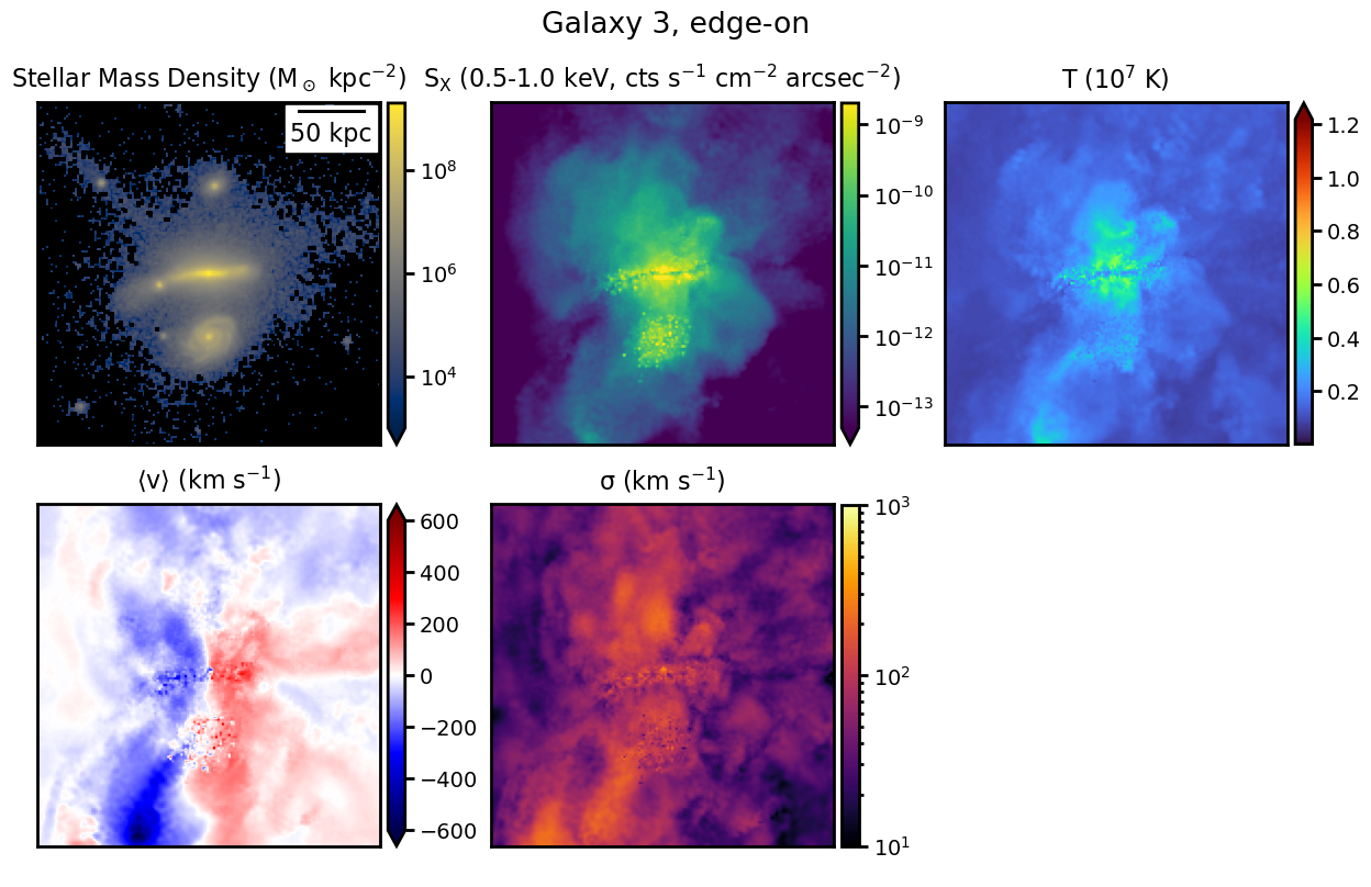
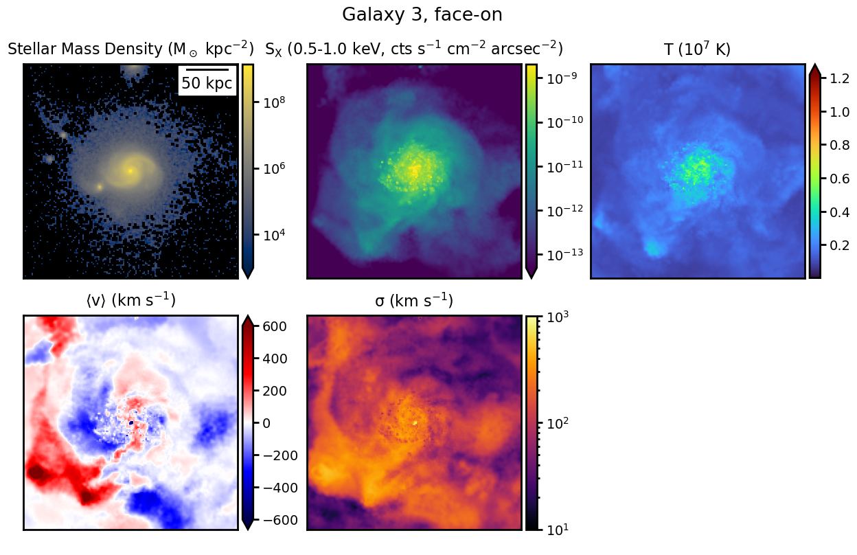
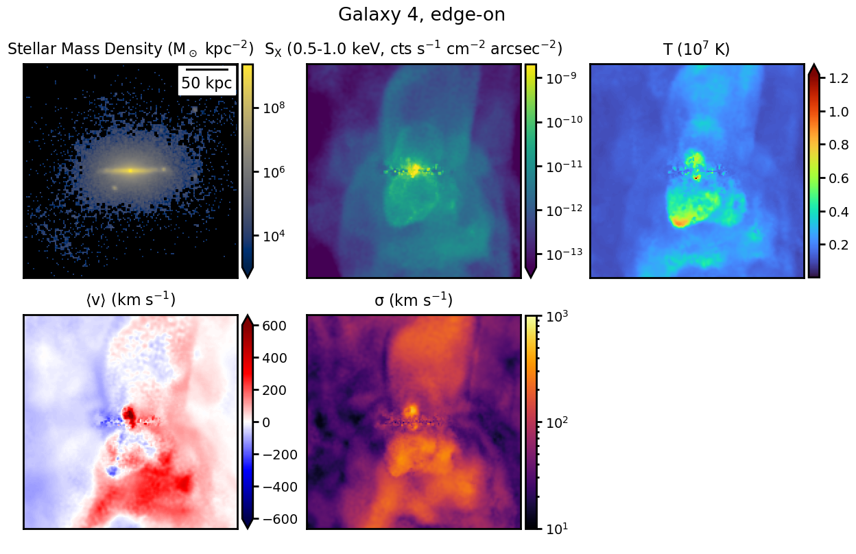
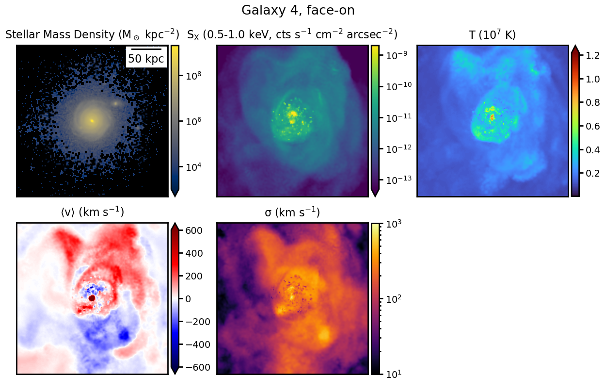
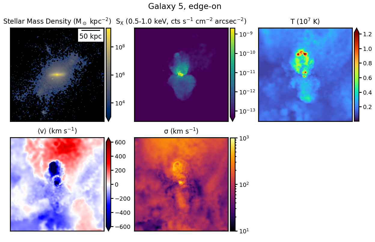
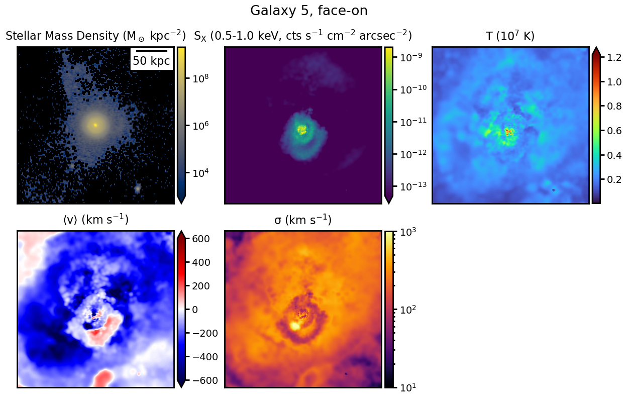
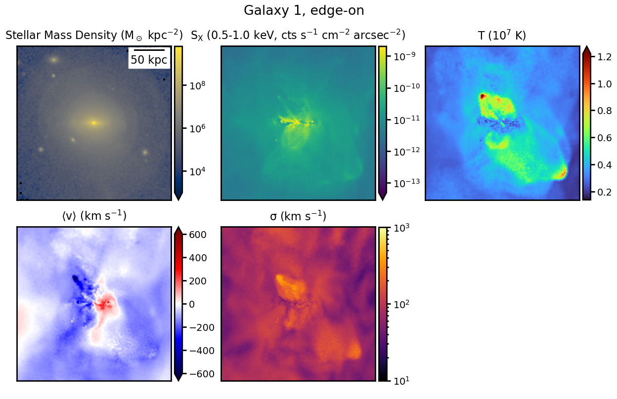
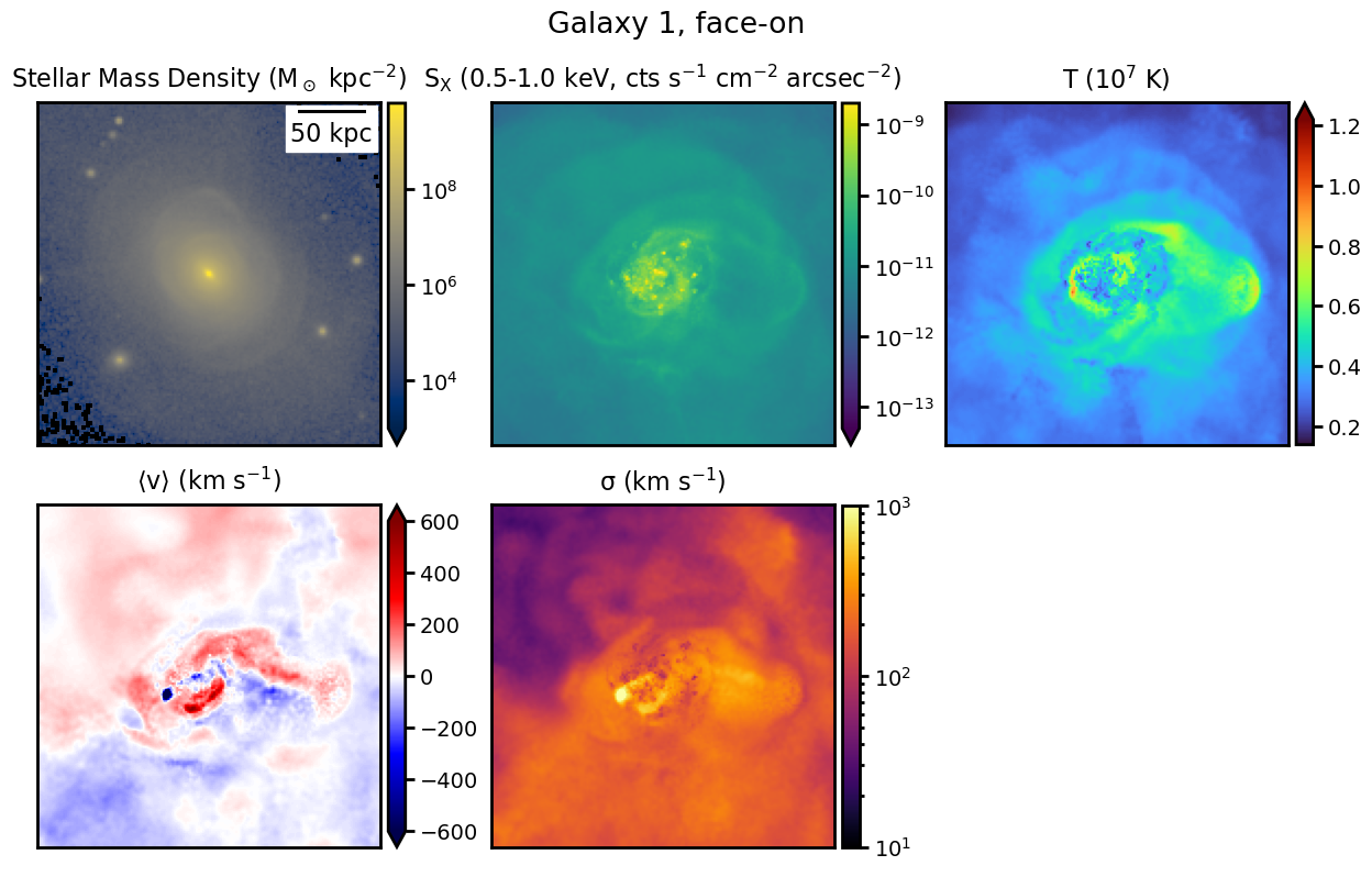
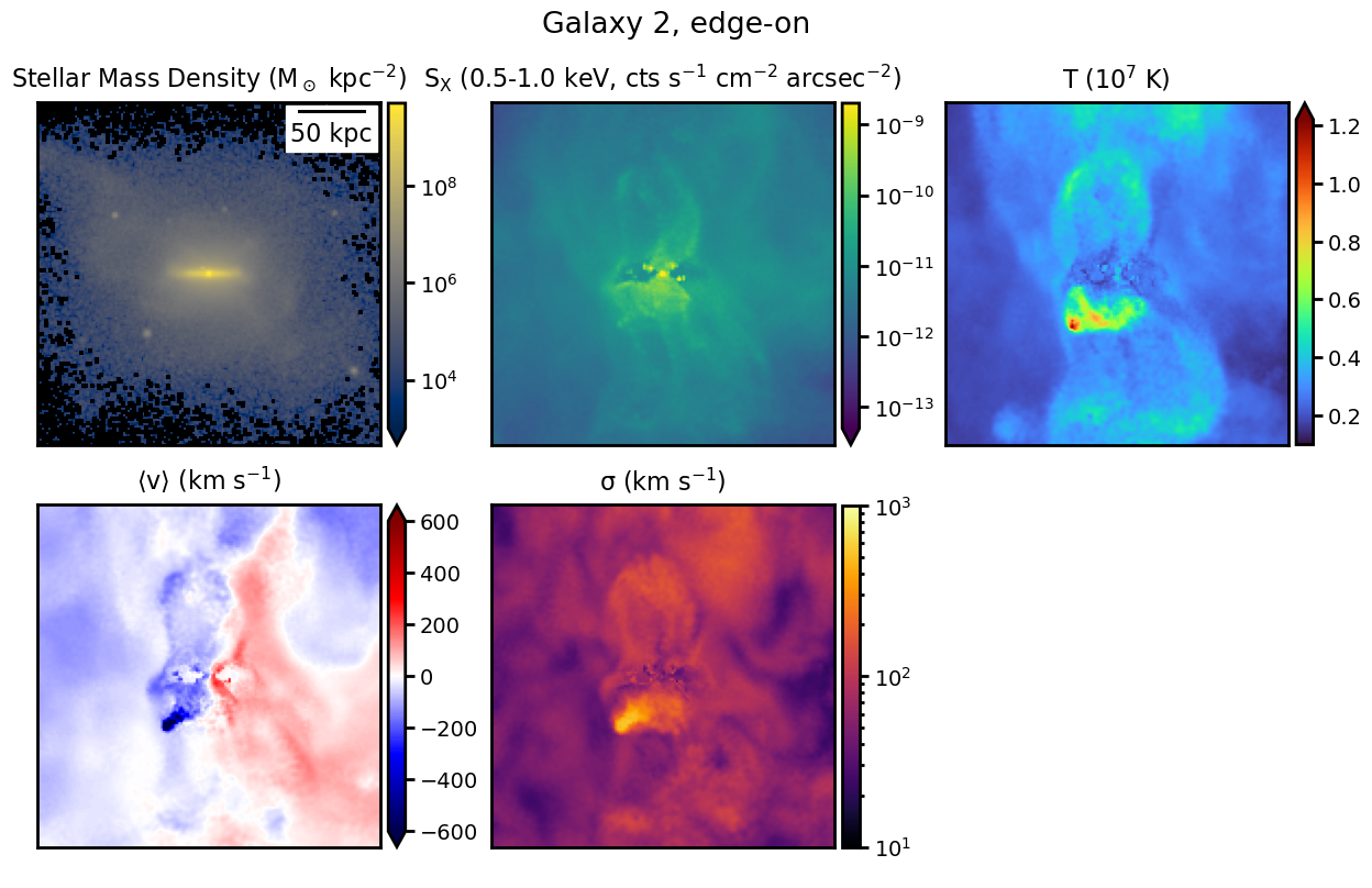
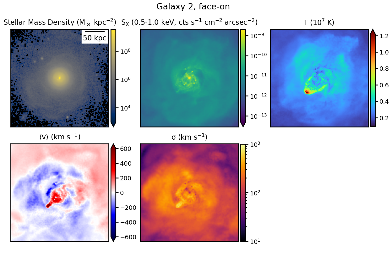
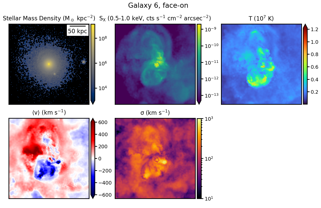
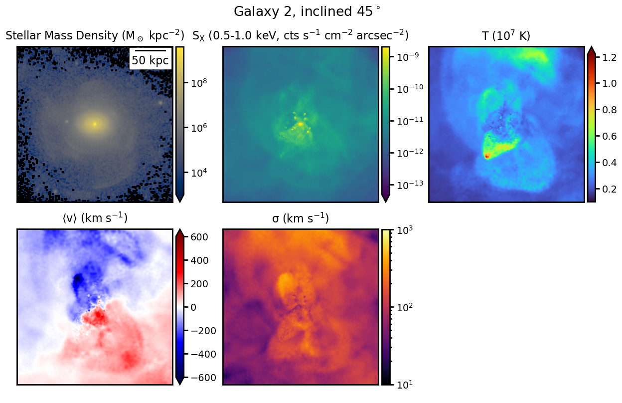
For three of the disk galaxies, we make projected maps of several quantities along the line of sight, which are shown in Figures 1-3. Each galaxy is projected along “edge-on” and “face-on” sight lines, defined with respect to the stellar disk. The top-left panel of each sight line of these figures shows projected stellar mass density. The stellar streams observed in both galaxies at large radii indicate past or ongoing merging activity with satellites.

The other four panels in each figure show projected quantities associated with the X-ray emitting gas. The top-center panels of each sight line of Figures 1-3 show X-ray SB in the 0.5-1.0 keV band, which spans the prominent emission lines for the hot CGM as noted in Section 1. In the edge-on projections (upper panels of Figures 1-3), there are clear indications in the SB maps of outflows perpendicular to the galactic disk, inflating cavities and entraining dense gas in their wake. The face-on projections (lower panels of Figures 1-3), do not show any such axisymmetry in their SB maps (as expected), but instead show roughly concentric edges along various directions, likely generated from the expansion of the outflowing gas perpendicular to the disk axis or from satellite merger activity.

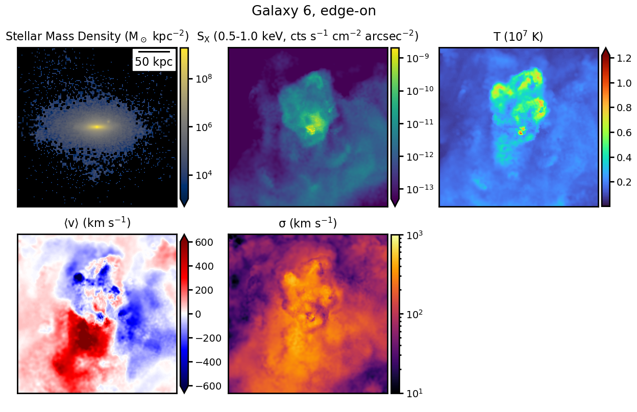
Much stronger indications of the nature of the various X-ray features can be seen in the projected temperature and velocity maps (which are weighted by the X-ray SB in the 0.5-1.0 keV band). Outflows are clearly associated with regions of higher temperature (top-right panels of Figures 1-3). Most of the hot CGM has a projected temperature of $T\sim 3.5-4.6\times 10^{6}$ K ( $\sim 0.3-0.4$ keV), whereas the regions associated with the outflows and bubbles in the SB maps range from $T\sim 5.8-11.6\times 10^{6}$ K ( $\sim 0.5-1.0$ keV).

The bottom-left panels of Figures 1-3 show the line-of-sight bulk velocity. In the edge-on projections of Figures 1 and 2 for galaxies 1 and 2, the mean velocity maps show clear signs of rotation of the CGM in the inner $r\sim 50$ kpc for both galaxies. Rotation speeds measure up to $\sim$ 200-300 km s^-1. Outside of this radius, the bulk flows do not tend to follow a clear pattern of rotation, and any measured velocities can be radial (whether inflowing or outflowing) or tangential. On the other hand, galaxy 6 (Figure 3) does not show a clear rotation pattern in the emission-weighted line-of-sight velocity map in the edge-on projection, instead exhibiting a complex pattern of velocities. Interestingly, it also does not show a symmetric pattern of outflows on either side of the galactic disk in the SB map, indicating that the hot outflow is not simply directed perpendicular to the disk in this particular case. The face-on projections of each galaxy show a complex pattern of mean velocities in both directions near the center of the galaxy, ranging from -600—600 km s^-1, indicating that though the majority of the flow is outward away from the disk, it is complex enough that in projection different sides of the galaxy may dominate in emission at particular spatial locations. At larger projected radii, the mean velocities are smaller, at $\sim$ -200—200 km s^-1.

The line-of-sight velocity dispersion maps are shown in the bottom-center panels of Figures 1-3. In the edge-on projections, velocity dispersions of $\sim$ 200-1000 km s^-1 are seen primarily in the regions dominated by the outflows. These correspond primarily to the expansion of bubbles and outflow regions along the sight line and not typically to regions of increased turbulence. In the face-on projections, the whole inner $r\lesssim 100$ kpc region has projected velocity dispersions of $\sim$ 300-1000 km s^-1, primarily due to the directed hot outflows on either side of the disk. This too is very patchy, reflecting the complexity of the outflows as seen in projection. Outside of these regions, the velocity dispersion is much smaller, around $\sigma\sim 100-200$ km s^-1. We will see later (Section 3.2) that the faster velocities (both mean and dispersion) near the center are associated with outflows, while the slower velocities at larger projected radii are associated with inflows.

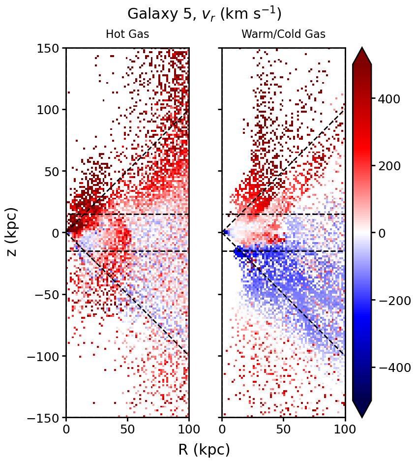
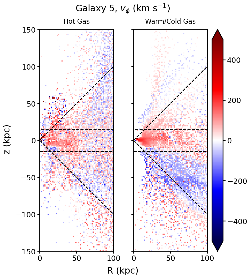
Projected maps in the face-on and edge-on directions for the other three galaxies (3, 4, and 5) are presented in Figures 21, 24, and 27 in Appendix A. In general, these maps show similar features in the different projections to galaxies 1, 2, and 6.

3.2 Velocity Profiles

In this Section, we further examine the properties of the CGM velocity field, focusing on outflows, inflows, and rotation. For this purpose, we adopt a cylindrical coordinate system where the vertical $z$ -axis is perpendicular to the disk, and the radial $R$ and angular $\phi$ directions define planes parallel to the disk. The origin of the coordinate system is defined to be at the center of the galaxy, where in particular $z=0$ defines the galactic plane. Note that in the following we will also refer to the coordinate $r=\sqrt{R^{2}+z^{2}}$ , which is the radial coordinate in the spherical coordinate system, as it is easier to distinguish inflows and outflows in this coordinate.

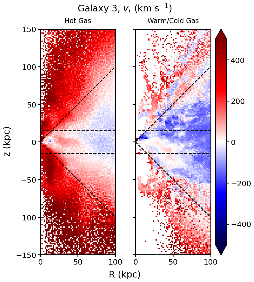
3.2.1 2D Velocity Profiles

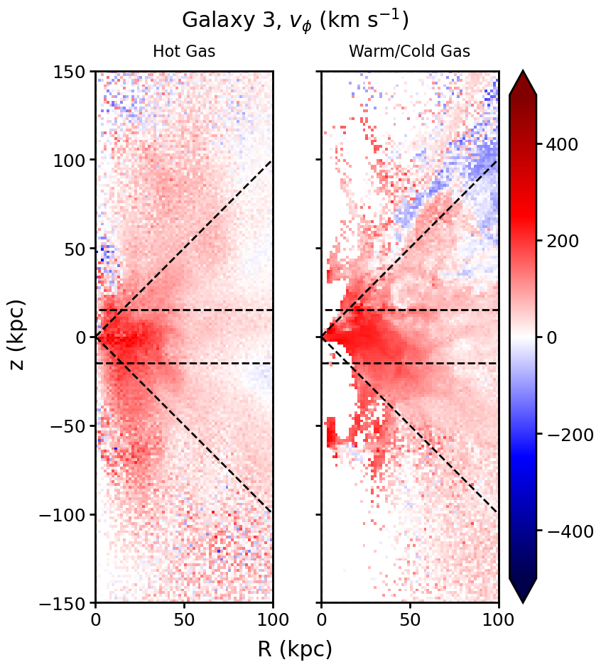
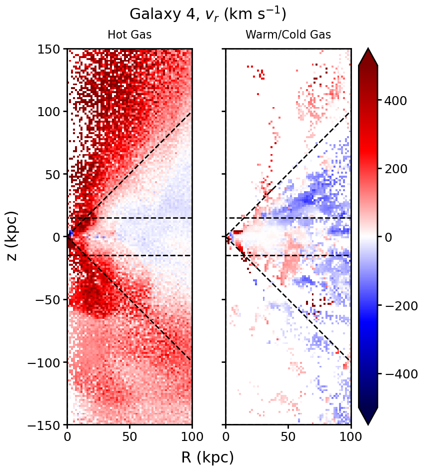
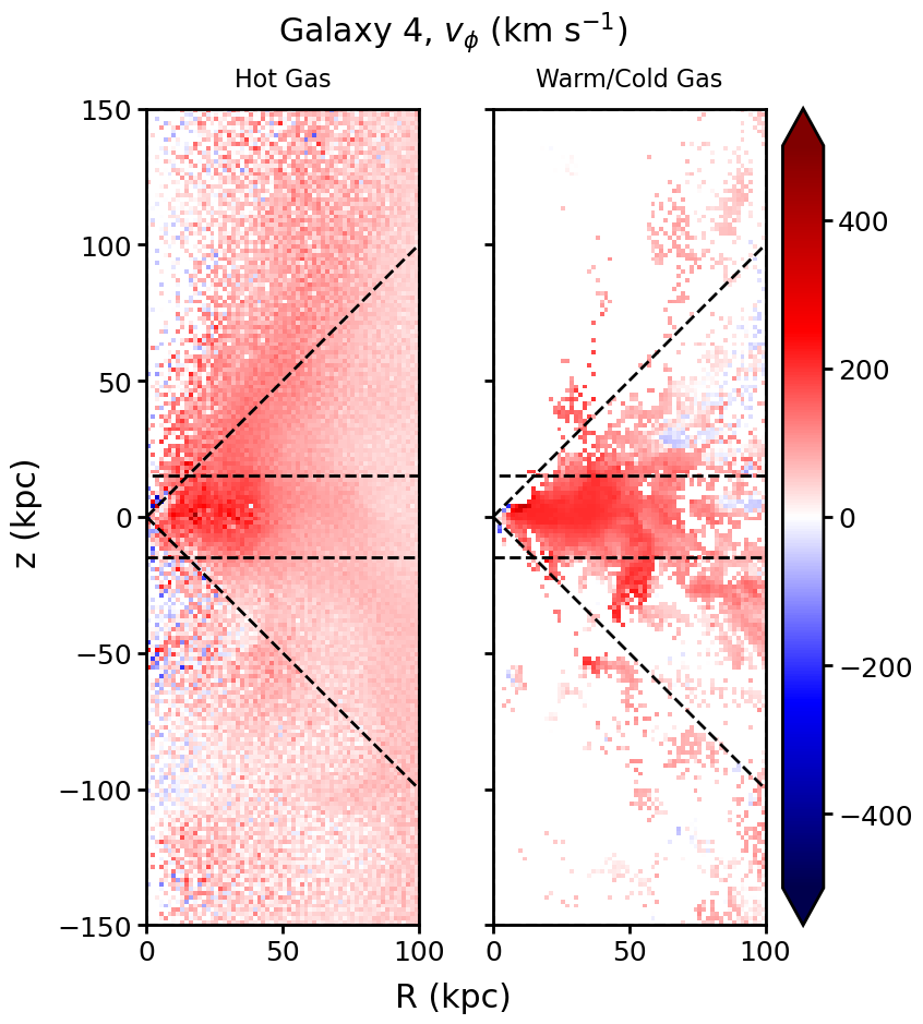
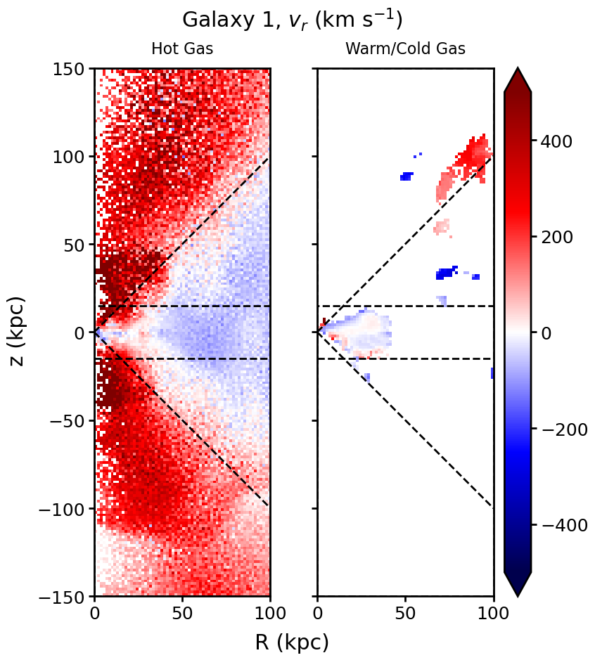
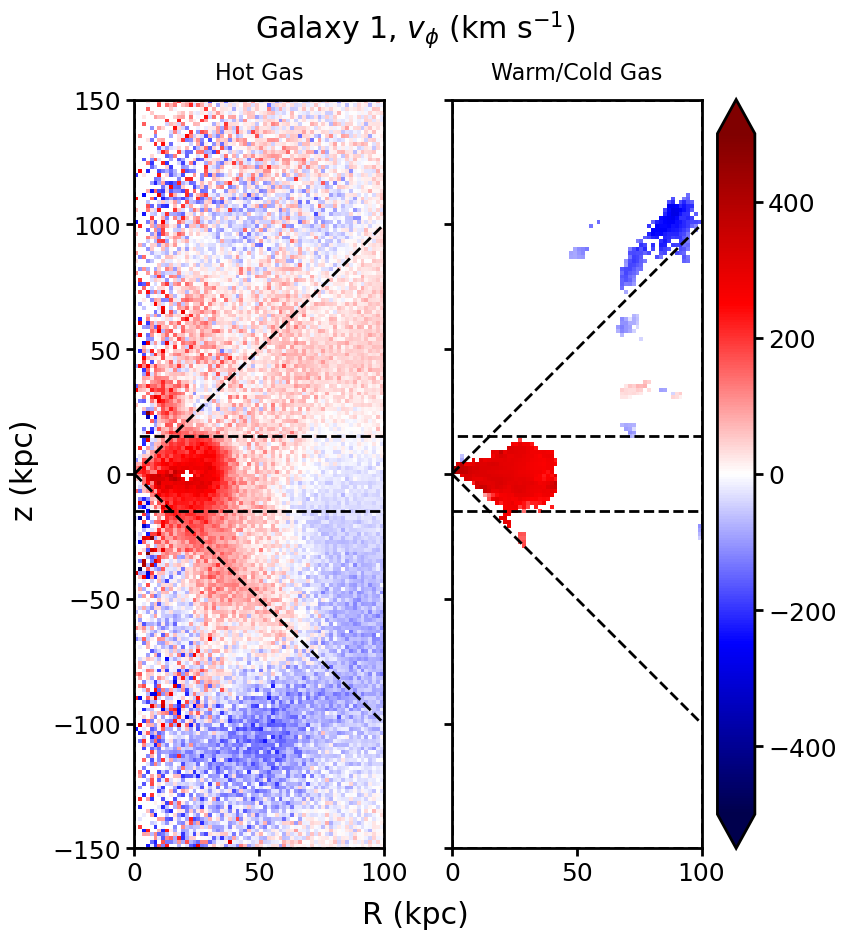
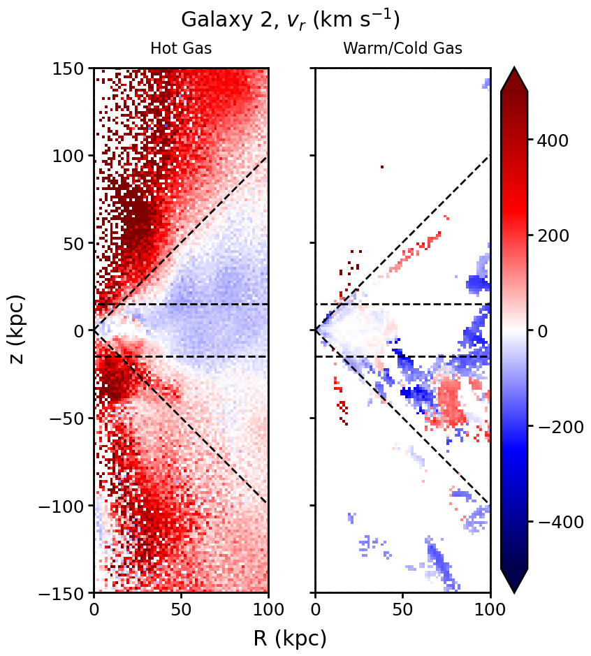
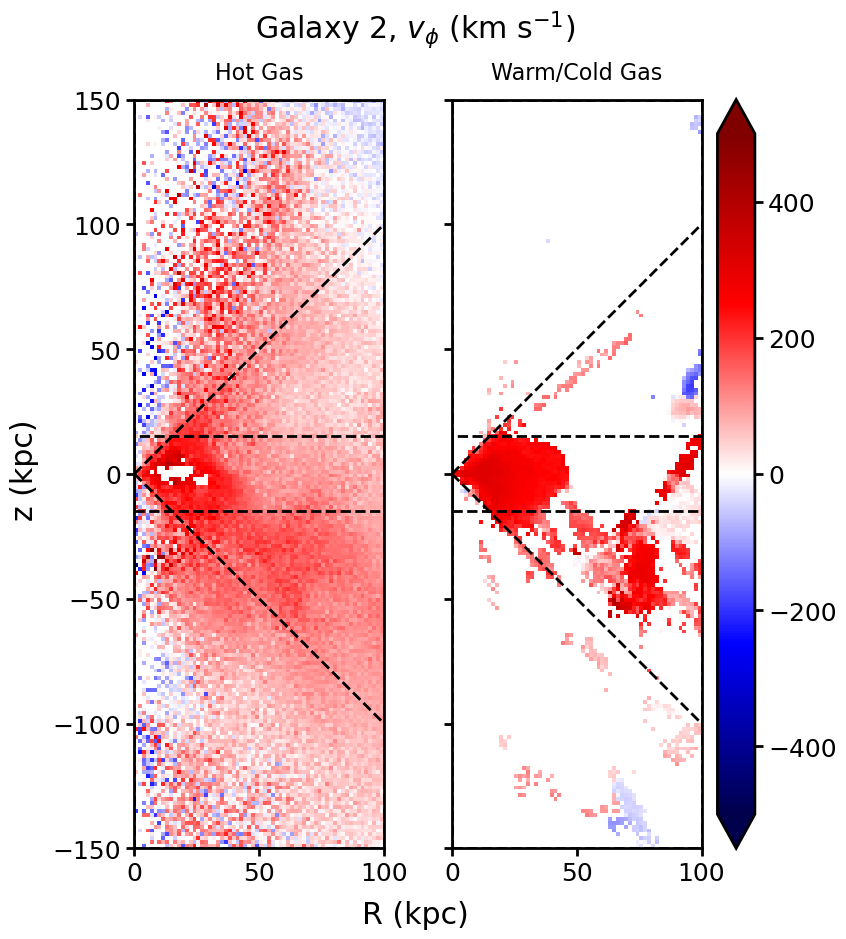
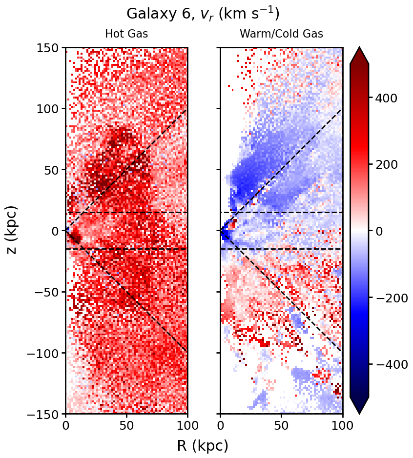
Figures 4-6 show 2D profiles of the mass-weighted velocity in the spherical- $r$ direction (left sub-panels), representing inflows and outflows, and the cylindrical- $\phi$ direction (right sub-panels), representing rotation and general tangential motions. The profiles are a function of $z$ and $R$ and are azimuthally averaged over the $\phi$ -direction, for both the “hot” ( $T\geq 5\times 10^{5}$ K) and “warm/cold” ( $T<5\times 10^{5}$ K) gas phases in both galaxies.

The left panels of Figures 4-6 show the azimuthally averaged mass-weighted spherical radial velocity $v_{r}$ for galaxies 1, 2, and 6. Galaxies 1 and 2 (Figures 4 and 5) display a straightforward geometry – in conical regions above and below the disk plane at $z=0$ , aligned with the $z$ -axis and with an opening angle of approximately 45^∘, the hot phase (left sub-panels) flows outward at speeds of $\sim$ 400-500 km s^-1 or more. These regions are dominated by feedback. The hot gas flows in this direction will be most easily observed in face-on disk galaxies, though the morphological features in X-ray SB and temperature which accompany these flows will of course be observed most easily in edge-on disk galaxies. This basic structure in SB and temperature in TNG50 galaxies was previously described in detail in Truong et al. (2021).

Outside of these conical regions, closer to the galactic plane, the hot phase is mostly slowly inflowing with a velocity of $\sim$ 100 km s^-1. In these two galaxies, there is not a significant amount of gas in the warm/cold phase, but it is largely confined to the volume away from the conical hot outflow regions and is mostly inflowing at velocities of $\sim$ 200-300 km s^-1. Galaxy 6 (Figure 6), however, is quite different. Essentially all of the hot phase is flowing radially outward at velocities of $\sim$ 300-500 km s^-1, and the warm/cold phase, which makes up a larger fraction of the mass of the CGM in this galaxy than galaxies 1 and 2, is mostly inflowing above the galactic plane and mostly outflowing below it, with similar speeds.

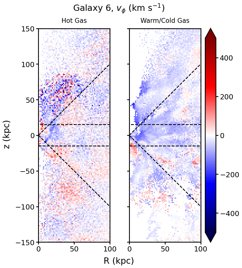
The right panels of Figures 4-6 show the azimuthally averaged mass-weighted velocity in the $\phi$ -direction. In galaxies 1 and 2, the hot phase (left sub-panels) shows coherent rotation of the CGM within a cylindrical radius of at least $\sim$ 50 kpc and a height above the disk out to $\sim$ 75 kpc, though for Galaxy 2 it extends somewhat further out. The majority of the warm/cold phase (right sub-panels) rotates in a disk of $\sim$ 50 kpc radius and $\sim$ 20-30 kpc thickness near the center, with other parts of the cold gas phase at large radii largely co-rotating with the hot phase. The rotation of the gas will obviously be most easily observed in edge-on disk galaxies. The hot phase in Galaxy 6 shows far less coherent rotation and instead is moving mostly randomly in the azimuthal direction, and very slowly with speeds of $\sim$ 50 km s^-1. The warm/cold phase has a more coherent rotation (though counter to the direction of rotation of the stars, see Section 3.2.2), with speeds of $\sim$ 100-200 km s^-1.

In summary, galaxies 1 and 2 are very similar, showing coherent hot outflows directed above and below the disk that push hot gas outward in the $R$ and $z$ -directions in conically-shaped regions on either side of the galaxy (as shown previously by Nelson et al., 2019a; Pillepich et al., 2021; Truong et al., 2021), while hot gas flows slowly inward closer to the galactic plane. Both galaxies also show coherent rotation of both phases, albeit at slightly different velocities (this will be explored more in Section 3.2.2). Galaxy 6 does not have any coherent rotation of the hot phase, and does not have any significant amount of gas which is inflowing. This is consistent with the disturbed appearance of the velocity field in the maps in Figure 3 in Section 3.1. Phase plots for the other three galaxies in the sample (3, 4, and 5) are shown in Figures 22, 25, and 28 in Appendix A. Galaxies 3 and 4 appear very similar to galaxies 1 and 2, whereas galaxy 5 appears more disturbed.

3.2.2 1D Velocity Profiles

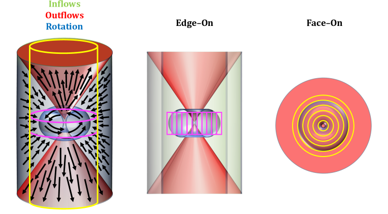
How are the properties of the velocity field seen in the 2D profiles in the previous Section and the properties of the velocity field in projection seen in the maps in Section 3.1 connected? To illustrate this, and to motivate the discussion in this and the following Sections, in Figure 7 we show a schematic representation of the major components of the velocity field for the galaxies in our sample (1-4) which have clearly distinguished regions of inflow (light green), outflow (light red), and rotation (light blue), shown in the left image with vectors indicating the directions of flow in the different regions. Given the cylindrical geometry, and the fact that X-ray spectra must be extracted over regions large enough to contain a statistically significant number of X-ray counts, two natural choices for regions to analyze the X-ray emission in cylindrical radial profiles in two different projections are also shown. The small magenta cylinder would be a logical choice for studying the radial profile of the rotation curve of the galaxy in the edge-on projection using line shifts, in which it would appear as a rectangular region (center image), where the smaller inset rectangles represent the radial bins and the regions from which spectra would be extracted. In addition to rotation in the inner hot CGM, in these regions the radial inflows in the outer regions would also have velocity components along the sight line, fully aligned with it at the very center and decreasing with projected radius. Assuming cylindrical symmetry, the radial inflow would produce a small line broadening, strongest near the center. In the face-on projection (right image), the larger yellow cylinder would represent measuring radial profiles in a set of circular annuli, which will probe the fast outflows near the center but also the slower inflows in the outer regions. Again assuming symmetry, both the outflows and the inflows would produce line broadening.

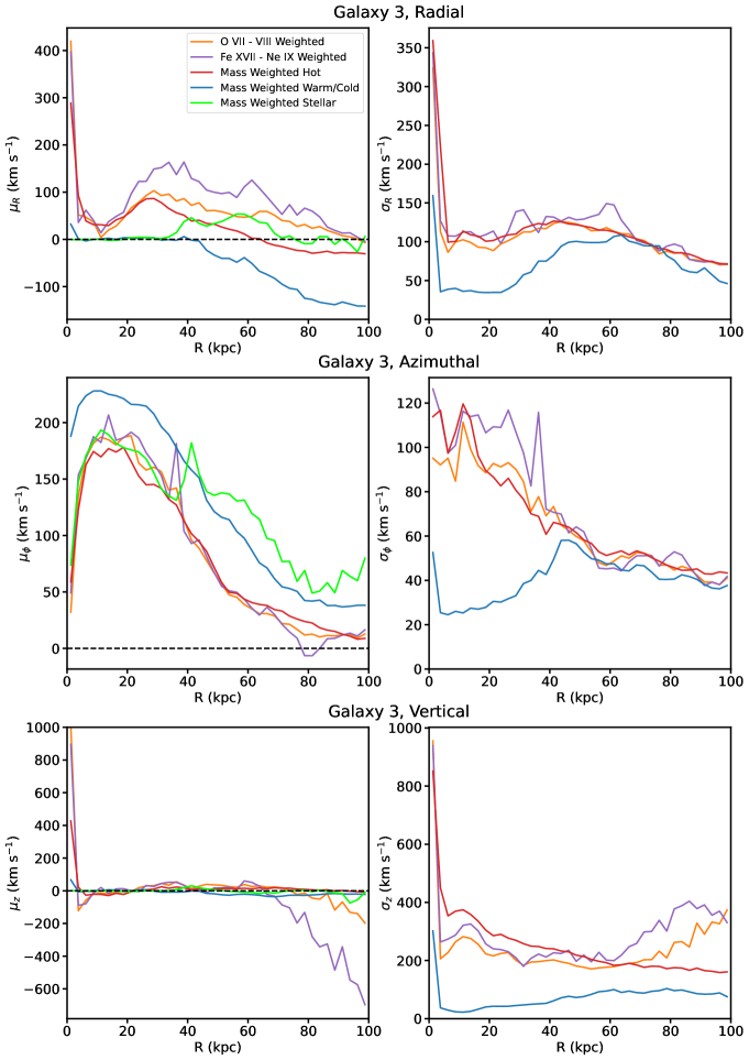
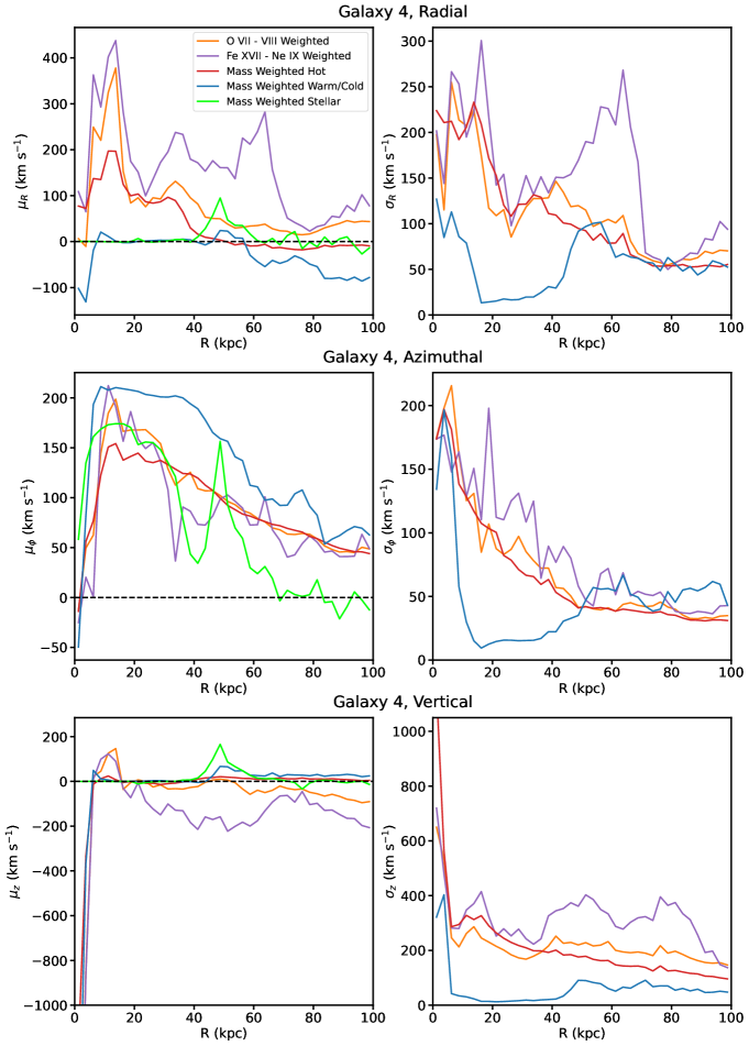
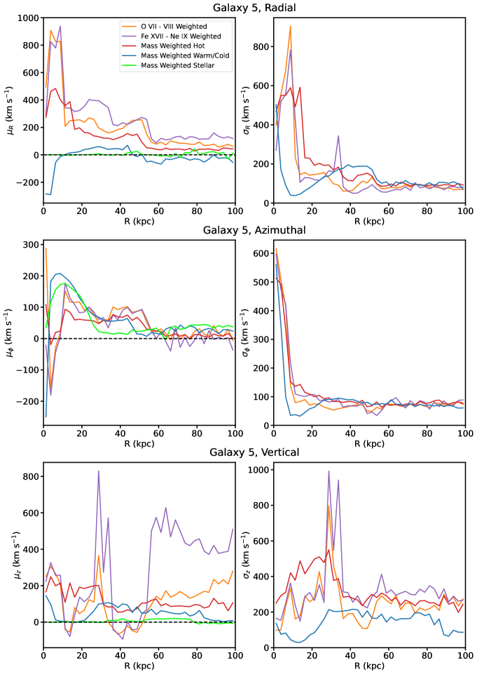
Motivated by these considerations, in this Section we produce azimuthally and height-averaged 1D profiles of the first two moments of the velocity field along the three coordinate directions $R$ , $\phi$ , and $z$ in the cylindrical coordinate system, as a function of cylindrical radius $R$ from the center of the galaxy. We also compare the profiles of the gas velocities to those from the stars. In what follows, for the $R$ and $\phi$ directions we extract 1D velocity profiles for the gas and stars (which will be viewed in edge-on projections) from a thin cylinder with a half-height of 30 kpc and radius of 100 kpc (represented by the magenta cylinder in Figure 7 and shown with dashed lines in Figures 4-5). For the $z$ -direction, we extract 1D velocity profiles (which will be viewed in the face-on projection) from a cylinder of the same radius but a half-height of 1000 kpc, which corresponds to a long cylinder with the axis projected along the line of sight (corresponding to the yellow cylinder in Figure 7).

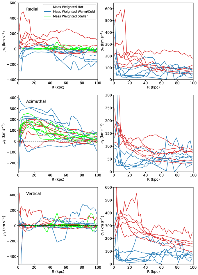
We first show mass-weighted velocity profiles of the stars (green), hot gas (red), and warm/cold gas (blue) for all six galaxies in Figure 8. The top panels of Figure 8 show the mean velocity (left) and the velocity dispersion (right) in the $R$ -direction. In this direction, a complication from the geometrical considerations discussed above immediately arises. For the galaxies with coherent hot outflows, the top and bottom of the thin cylinder used to extract the profiles (30 kpc away from the galactic plane) intersects with the boundary of this outflow at a radius of roughly $\sim$ 30-50 kpc (see Figures 4-5). Within this radius, the hot phase is outflowing with an average velocity $\mu_{R}\sim+50-200$ km s^-1. Outside of this region, the hot gas is either outflowing with a similar velocity, or inflowing with $\mu_{R}\sim-50-100$ km s^-1, depending on whether this phase has the simple outflow/inflow structure, which is the case for galaxies 1, 2, 3, and 4. The warm/cool phase gas, regardless of radius, is mostly inflowing with an average velocity of $\mu_{R}\sim-100-300$ km s^-1. The velocity dispersion in the radial direction is typically larger for the hot phase, with $\sigma_{R}\sim 100-500$ km s^-1, than the warm/cold gas, which has $\sigma_{R}\sim 50-100$ km s^-1.

The middle panels of Figure 8 show the same profiles for the $\phi$ -component of the velocity. The middle-left panel shows the mean $\phi$ -velocity–essentially the rotation curves of the different phases. Though there is a clear spread, in general the rotational speed of the cold gas is faster than the hot gas within a radius of $\sim$ 50-kpc, with the former rotating at $\sim$ 200-400 km s^-1 and the latter rotating at $\sim$ 50-200 km s^-1. The stellar disks are rotating at $\sim$ 100-200 km s^-1. The middle-right panel shows that the $\phi$ -velocity dispersions within $\sim$ 50 kpc for the hot gas are slightly higher than the cold gas– $\sim$ 100-150 km s^-1 versus $\sim$ 50-100 km s^-1, respectively. The lack of complete rotational support for the hot CGM in these TNG50 galaxies is consistent with previous results from other works (Oppenheimer, 2018; Huscher et al., 2021; Hafen et al., 2022). We also note the fact that there is more angular momentum in the warm/cold gas than the stars, in agreement with previous studies (e.g. Oppenheimer, 2018) and shown to be common to simulations of galaxy formation by Stewart et al. (2017), arising at least in part from cold, high-angular-momentum streams of infalling gas.

The bottom panels show the same profiles in the $z$ -direction, which would be seen if a galaxy were viewed face-on. The mean $z$ -velocity profile hews very closely to zero for nearly all of the profiles. This is expected if the outflows are nearly equal and opposite on either side of the disk in galaxies observed face-on. Exceptions to this are most prominent in the very center ( $r\lesssim 10-20$ kpc), where the volumes of the radial annuli are small enough that the average can dominated by a few cells with high velocity (see also the bottom-left panels of Figures 1-3 in Section 3.1, which show large velocity shifts near the center). Deviations from zero velocity mean are more pronounced in the warm/cold phase, which is sometimes dominated by large and coherent parcels of gas (see the phase plots in Section 3.2.1). The $z$ -velocity dispersion profiles show a clear separation between the hot phase and the warm/cold phase–the former has velocity dispersions within $\sim$ 40 kpc of $\sim$ 300-500 km s^-1, and the latter has very low dispersions of $\lesssim$ 100 km s^-1, with one outlier curve with a dispersion of $\sim$ 200 km s^-1 (galaxy 5) over almost the entire radial range. The high dispersions in the hot phase come from the oppositely directed outflows on either side of the galaxy.

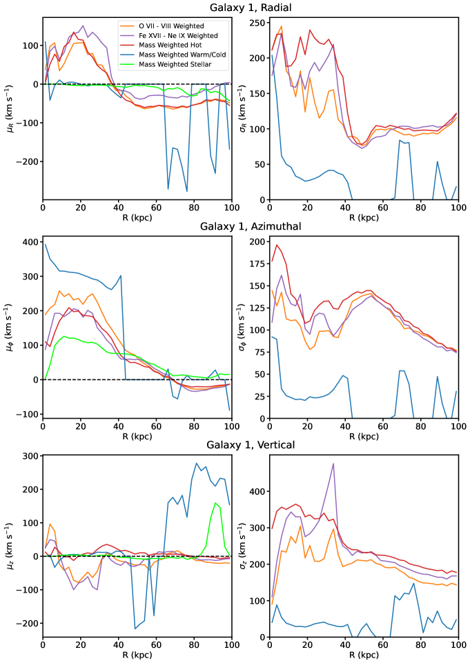
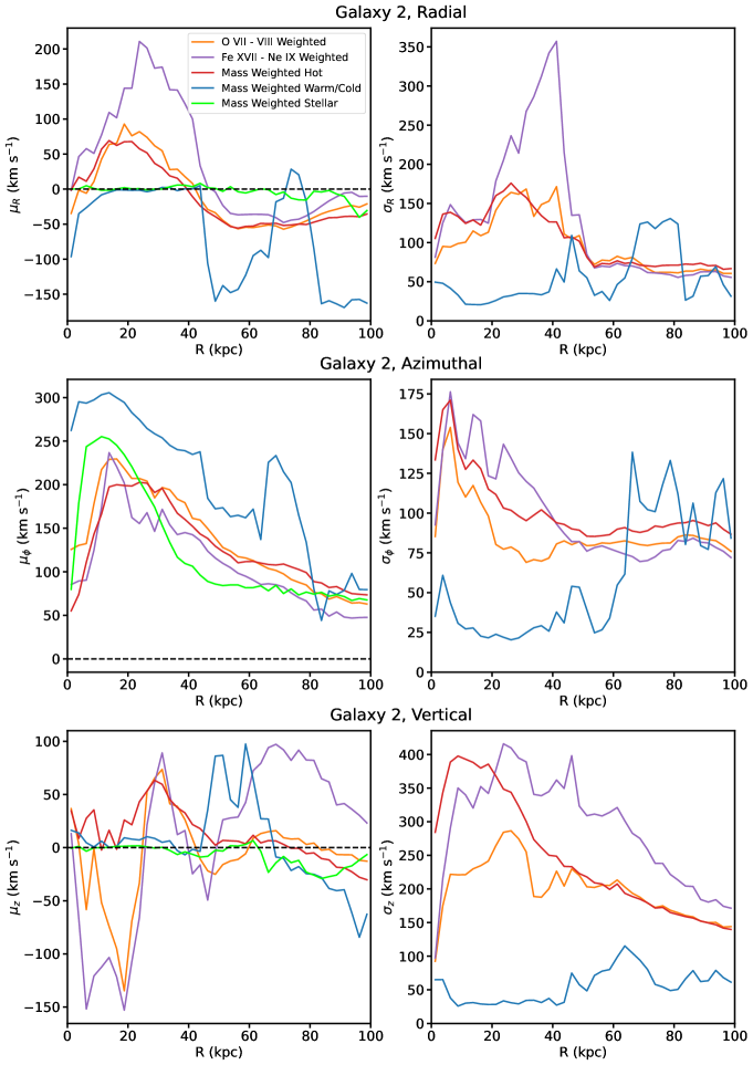
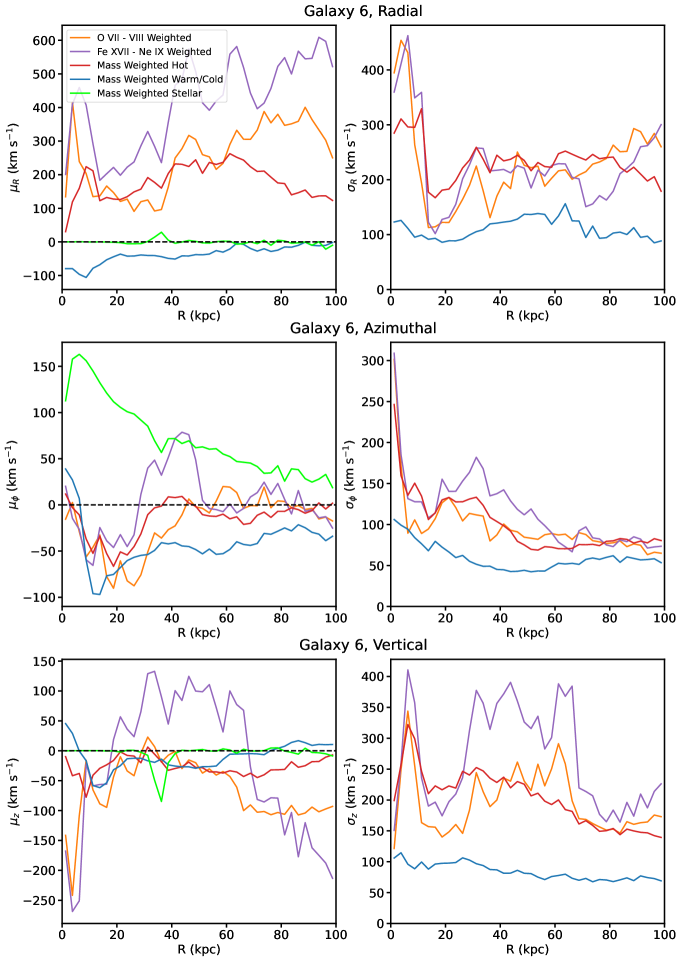
We now briefly look in more detail at the 1D velocity profiles of the individual galaxies. These are shown for galaxies 1, 2, and 6 in Figures 9-11. Here, we also show the velocity profiles for the hot gas weighted by the X-ray emission in specific source-frame bands around prominent emission lines in the CGM: O VII and O VIII (0.558-0.656 keV band, orange lines), and Fe XVII and Ne IX (0.723-0.924 keV band, purple lines). These weightings are significant since they correspond more closely to what X-ray microcalorimeter instruments will be able to measure. The arrangement of the panels in Figures 9-11 is the same as in Figure 8.

In the top panels of each figure, we show the first and second moments of the $R$ -component of the velocity. For galaxies 1 and 2 (Figures 9 and 10), the hot gas is outflowing within $\sim$ 50 kpc with a velocity up to $\sim$ 100-200 km s^-1, depending on the weighting used. For example, in galaxy 2 the hotter gas probed by the higher-energy emission lines of Fe XVIII and Ne IX is moving faster than both the cooler hot phase probed by the lower-energy O emission lines, as well as the gas probed by the mass weighting. At these inner radii, this is indicative of the hot, outflowing gas from the central SMBH. The warm/cold phase in this region has essentially zero radial velocity. Beyond this radius in these two galaxies, the hot gas is inflowing at $\sim$ -50-100 km s^-1, with slightly slower speeds for the phase weighted by the Fe VIII-Ne IX emission. Parcels of warm/cold gas are also inflowing at these radii with higher velocities near $\sim$ 150-300 km s^-1. Galaxy 6 is very different in that the hot gas is strongly outflowing at all radii with velocities of $\sim$ 100-400 km s^-1 depending on the weighting. The cold phase is inflowing at all radii, especially near the center, with velocity up to $\sim$ 100 km s^-1.

In the $\phi$ -direction (middle panels of Figures 9-11), the mean and dispersion of the velocity between the different weightings for the gas are all more similar for galaxies 1 and 2. This is expected, since the azimuthal direction is least affected by the hot outflow. Galaxy 6 is once again seen to be quite different from the other two–both its warm/cold and hot phases are counter-rotating in the direction of the stars.

The bottom panels of each figure shows the moments of the $z$ -component of velocity. We note again (as seen in Figure 8) that in this projection the mass-weighted mean velocities of both the hot and warm/cold phases are close to zero (as expected), and that the mass-weighted velocity dispersion is higher for the hot phase. In the emission-weighted profiles, the absolute value of the mean $z$ -velocity can be significant in places, up to $\sim$ 150 km s^-1. Similar to the $R$ -component, the velocity dispersion in the $z$ -direction weighted by the Fe XVIII and Ne IX lines can be noticeably higher than that weighted by the O lines. Similar trends between the profiles are seen in the other three galaxies (3, 4, and 5), as seen in Figures 23, 26, and 29 in Appendix A.

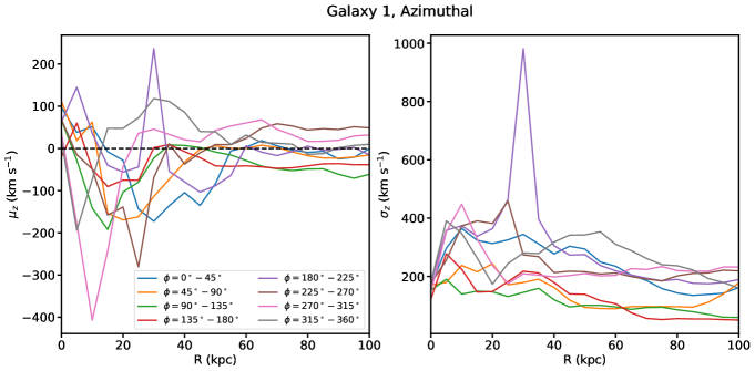
As already noted, azimuthally averaged profiles such as these are motivated not only by the geometry but also by the number of X-ray counts available for an observation. This immediately introduces a complicating factor–the mean and the standard deviation of the velocity in such a large region may either arise from the velocity distribution along the sight line or from the velocity distribution across the sky plane within the region. To check for this effect, we plot profiles of the velocity in the $z$ -direction for Galaxy 1 in the face-on projection in 8 different azimuthal sectors of width 45^∘ each in Figure 12 (to be compared to the top panels of Figure 9.) This figure clearly shows that there is an effect on both the measured velocity mean and dispersion from the azimuthal averaging (which can also be predicted from the bottom panels of Figure 1). This should be taken into consideration when interpreting the results of the azimuthally averaged profiles, and mitigated by splitting into subregions if there are enough counts to do so.

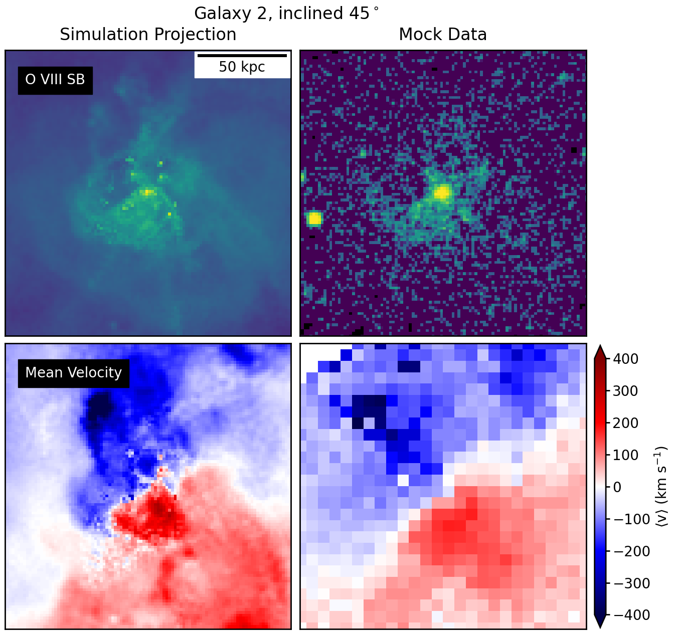
3.3 Off-Axis Projections

Of course, most galaxies will not be inclined either perfectly edge-on or face-on to our sight line. In off-axis projections, components of the velocity field from both the rotating CGM and the hot outflows will be observable together. In the two projections we have examined so far, the outflow velocities could not be easily measured via line shifts, either because they were mainly out of the sight line in the edge-on case, or in the face-on case the oppositely directed outflows largely canceled out the overall line shift. In the case of an off-axis projection, these outflow velocities could be measured, and if the inclination angle can be constrained from the stellar disk the total outflow velocity may be estimated.

Figure 13 shows maps of the same quantities as shown in Section 3.1, except along a sight line 45^∘ away from both the edge-on and face-on projections, for galaxy 2, to give an example. The most intriguing of these images are the projected mean velocity maps (bottom-left panels for each galaxy). The outflow velocities on either side of the galaxy are clearly seen, and can be spatially matched with features in X-ray SB (top-middle panel for each galaxy) showing outflows and cavities. The pattern of the velocity field in the map is also twisted from a purely vertical dipole, showing the effect of both CGM rotation and outflows in the same projection.

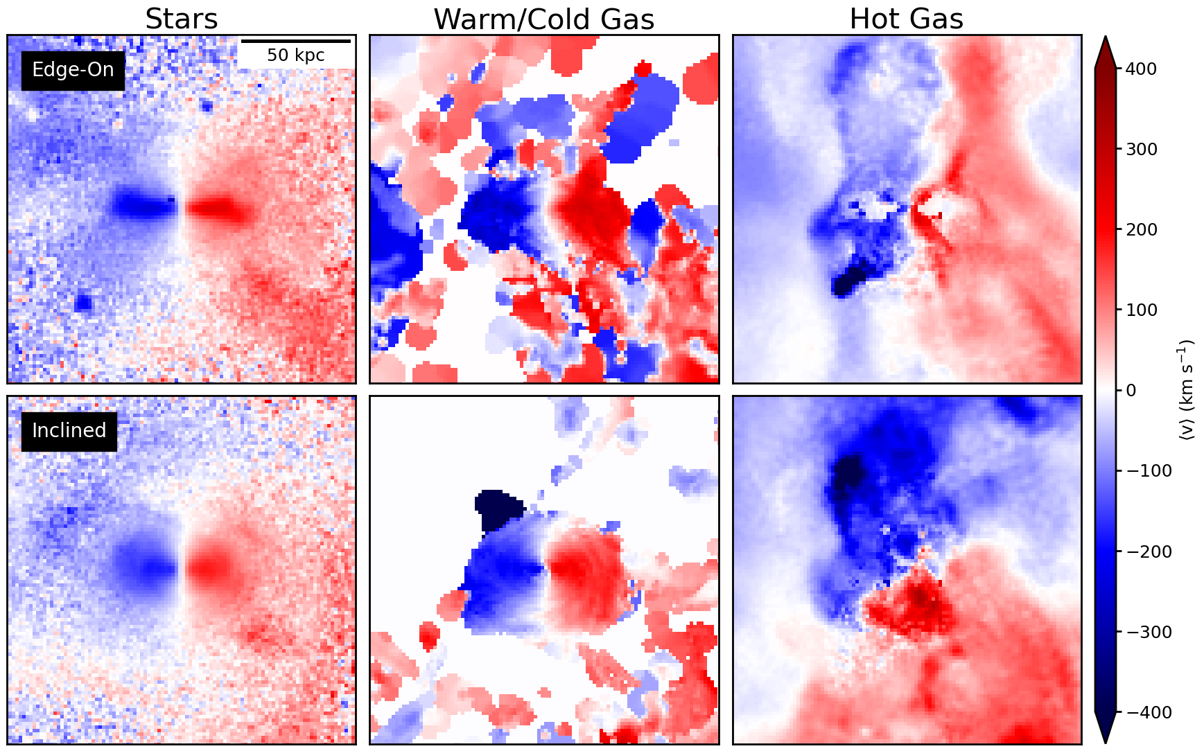
This last effect is particularly interesting, as it reveals how the different baryonic phases can have very different kinematic properties. Figure 14 shows line-of-sight mean velocity maps for the stars and warm/cold and hot gas phases, for both the edge-on and inclined projections. In the edge-on projection, the stars and both gas phases show a common rotation pattern in the inner $\sim$ 30 kpc region of the galaxy, though they may rotate at slightly different speeds as noted in Section 3.2. In the inclined projection, though the stars and warm/cold gas show the same axis of rotation as before, the velocity pattern of the CGM is tiltled with respect to both due to the hot outflow signature combined with the rotation signature. This is an intriguing prediction which can only be tested with an X-ray microcalorimeter.

3.4 Mock X-ray Observations

In this Section, we produce synthetic X-ray observations of galaxies 1 and 2 using the procedure described in Section 2.2, using a model with instrument characteristics similar to LEM (Kraft et al., 2023). In the spectral analysis that follows, the brightest $\sim$ 50-100 CXB point sources have been identified using wavdetect (Freeman et al., 2002) and removed.

3.4.1 Velocity Maps from Spectral Fitting

If statistics permit, X-ray IFUs will be most useful in producing maps of projected quantities from model fits to spectra. To demonstrate this, we carry out such a procedure on two of our model event files to produce maps of line-of-sight mean velocity. This analysis is carried out using the CIAO (Fruscione et al., 2006) and Sherpa packages (Burke et al., 2020).

We first extract a spectrum from a region by removing all emission within a radius of 12.5’ from the galaxy center. We fit this spectrum to a combined model for the MW foreground (apec + TBabs*(bapec+bapec), where TBabs is the same foreground absorption model described in Section 2.2, and bapec is an APEC CIE model with thermal line broadening), one power-law component for the (unresolved) CXB, and another for the NXB.

With the background determined, we proceed to produce the velocity map. We then bin the counts images in the O VIIf⁵⁵5Only the O VII forbidden line is sufficiently redshifted away from the MW foreground lines at $z=0.01$ to be used for this purpose., O VIII, and Fe XVII lines (defined by narrow bands around the line centroids at $z=0.01$ with width 3 eV) into 30” pixels (twice the size of the pixels in the simulated instrument). Each of these larger pixels is the center of a circular region where the radius is expanded until it reaches a SNR of 7, where the maximum allowed radius of each circle is 4.5’ (18 pixels). Spectra are extracted from these regions, and grouped so that there is at least one count in each energy bin of the spectra.

Each circular region is then fit to a single-component TBabs*bapec model for the source, with the parameters for the model components corresponding to the MW foreground and the NXB frozen to the values obtained from the background-only fit (rescaled by area), and the normalization of the CXB component free to vary to account for the variable CXB contributions in each localized circular region. We fit each spectrum in 8 eV bands around the O VII, O VIII, and Fe XVII lines. For the source model, the temperature, redshift, line width, and normalization parameters are free to vary. The hydrogen column density for foreground galactic absorption is fixed to $N_{H}=1.8\times 10^{20}$ cm^-2, and the abundance parameter is fixed to $Z=0.3~{}Z_{\odot}$ , assuming Anders & Grevesse (1989) relative abundances. These parameters are fixed given the narrow spectral bands we use in the fits; neither of them will be well-constrained by the fit and the measurement of the line shift is not sensitive to their value in any case. We fit by minimizing the Cash statistic Cash (1979). Once a best fit for a region is found, we refine it by running a Markov Chain Monte Carlo (MCMC) analysis with 2500 steps.

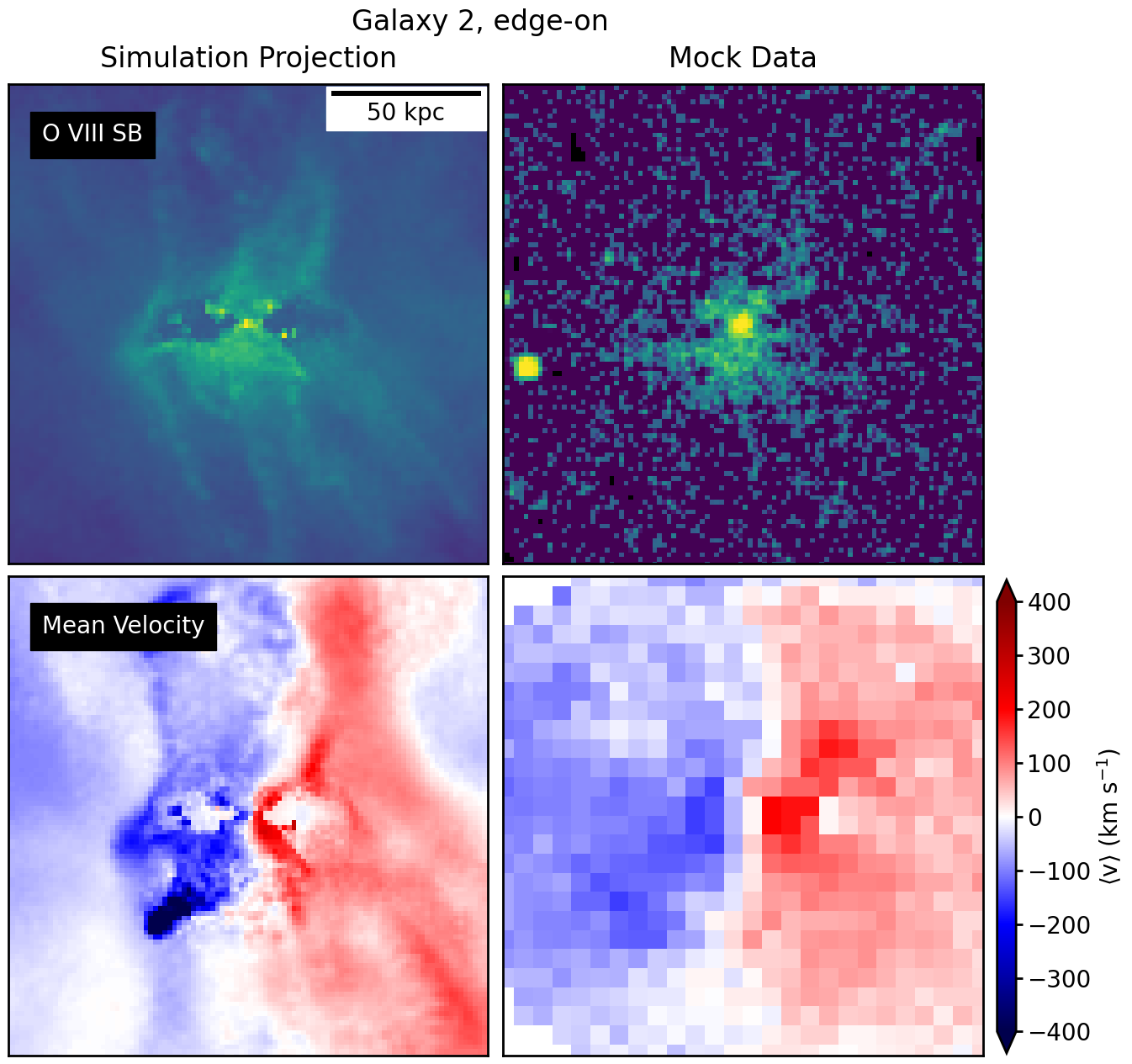
Figure 15 shows the result of this procedure on the observation of galaxy 2 with the sight line facing edge-on (left subpanels) and inclined 45^∘ to the plane of the galactic disk (right subpanels). The top subpanels show maps of SB in the O VIII line, with the idealized SB map projected from the simulation in the top-left subpanels and the counts map from the mock observation in the top-right subpanels. The bottom subpanels show the line-of-sight mean velocity, computed from the simulation by weighting by the emission in the 0.5-1 keV band (bottom-left subpanels), and produced from the fitted line centroid as described above (bottom-right subpanels). Typical uncertainties on the mean velocity from the fits are $\pm 20-30$ km s^-1. There is remarkable agreement between the simulated and fitted velocity maps, with the model fits reproducing the overall shape of the velocity distribution as well as the magnitude of the velocity in either direction. The absolute values of the most extreme values of the idealized map are slightly underestimated due to the fact that they appear in small regions with faint emission that do not contribute greatly to the spectra in their respective circular regions. The reproduction of the general features in the map demonstrates that an X-ray IFU with $\sim$ 1 eV spectral resolution will be able to map the velocity field of the CGM to sufficient detail to observe the effects of rotation and outflows.

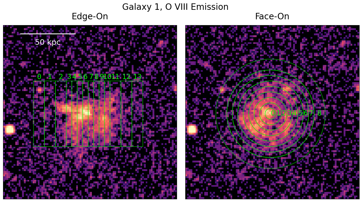
3.4.2 Velocity Distributions in Regions from Spectral Fitting

Figure 16 shows a 1 Ms exposure of galaxy 1 in the face-on and edge-on projections, where the plotted events have been restricted to the 0.646-0.649 keV band, which bounds the redshifted O VIII line at z = 0.01. As noted in Section 2.2, all backgrounds are included in this image. Also overlaid on the two panels in Figure 16 are numbered regions from which spectra are extracted for fitting to emission models for the analysis in Section 3.4.2. In the edge-on image (left panel), the regions are made of rectangles so that the velocity profile of the CGM can be measured across the disk. In the face-on image, the regions are made of annuli, reflecting the approximate cylindrical symmetry along this sight line.

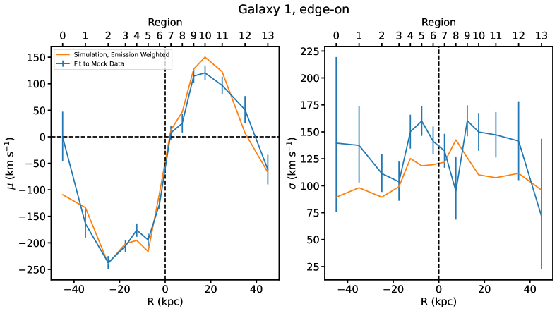
We extract spectra from the regions shown in Figure 16 and fit them using XSPEC (Arnaud, 1996). In each region, we model the CGM emission using a single TBabs*bapec component, where the hydrogen column density for foreground galactic absorption and the metallicity parameters are fixed as above, and the temperature, redshift, velocity broadening, and normalization parameters are free to vary. For the galactic foreground emission, we assume the model given in Section 2.2, holding all parameters fixed except an overall constant normalization which is free to vary. A power-law component is included to model the CXB, with its photon index and normalization parameters free to vary. Finally, the normalization of the constant particle background component is also free to vary. We fit within the 0.64-0.83 keV band (covering the O VIII and Fe XVII lines), and use the Cash (Cash, 1979) statistic for minimization.

The result is shown in Figure 17, where the blue lines show the mean (left panel) and standard deviation (right panel) of the velocity as determined from the spectral fitting, and the orange lines show the same quantities projected directly from the simulation weighted by the X-ray emission in the 0.5-1.0 keV band. The shape of the mean velocity measurements clearly shows the rotation curve, and is in excellent agreement with the simulation projection and broad agreement with the azimuthally averaged curve of the same quantity in the middle-left panel of Figure 9. The measured velocity dispersion is also in broad agreement with the simulation projection. For the reasons discussed in Section 3.2.2, this quantity will be dominated by the oppositely directed radial ( $R$ ) inflows near the center of the galaxy, while at larger projected radius the contribution of differences along the azimuthal ( $\phi$ ) direction will become more important. The numbers measured here are consistent with those from the 1D radial profiles in the top-right and middle-right panels of Figure 9.

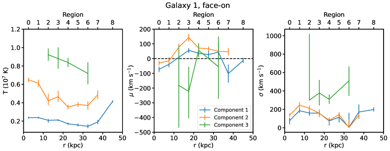
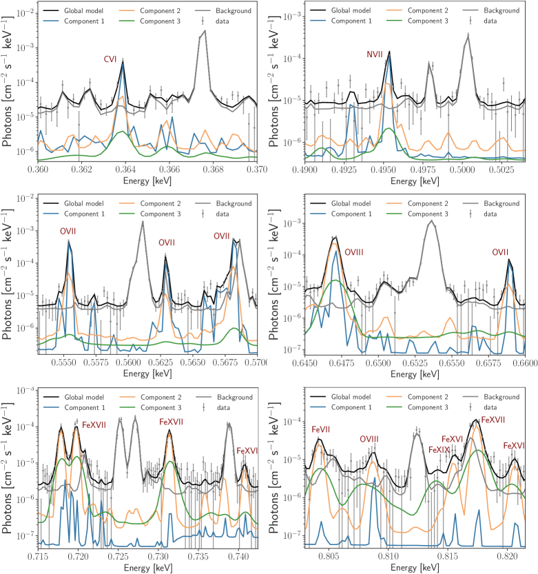
For the face-on projection, the story is somewhat different. In this case, where we project along the $z$ -axis of the cylinder, there is a complex distribution of outflows and inflows with different temperatures and velocities. As we have already seen (Figure 12), azimuthally averaging within an annular region also combines different phases in a non-trivial way. We find for many of the annular regions shown in Figure 16 that a single thermal emission model component does not adequately represent the observed emission from the CGM within them. To this end, we have fit these 9 regions with multiple components to attempt to capture multiple temperature and velocity components in the hot gas from both the outflows and the inflows, which we would predict to be observed especially along this sight line from the results of Sections 3.1 and 3.2. For these fits, we have successively added additional bapec components until no more components were statistically required. In order to make sure we can also correctly detect and characterize weaker emission components, we used the whole energy range (0.3-2 keV) and kept background parameters free to vary in this part of the analysis. This kind of deep, multi-component analysis will only be possible with microcalorimeter-quality data.

The results are shown in Figure 18, for which all regions are numbered for reference back to Figures 16. The left panel shows the fitted gas temperature for each region, for fits with 1, 2, and/or 3 bapec components. Not all of the annular regions were well-fit by a second or a third component—only regions where a new component was statistically required are shown. It can be seen that there are three distinct gas temperatures recovered by the fits (left panel)—the dominant Component 1 is at $T\sim 2.3\times 10^{6}$ K, ( $\sim 0.2$ keV), with Component 2 at $T\sim 4.6-5.8\times 10^{6}$ K ( $\sim 0.4-0.5$ keV), and Component 3 at $T\sim 7.0-9.3\times 10^{6}$ K ( $\sim 0.6-0.8$ keV). The mean velocities for these three components are shown in the center panel, with Components 1 and 2 averaging around zero velocity with a range of $\sim-100-100$ km s^-1. Component 3, which is the hottest gas, has mean velocities as high as $\sim-200$ km s^-1 near a radius of $\sim$ 10-20 kpc, but these values are also more uncertain. The right panel shows the velocity dispersion for each component, which is $\sim$ 100-200 km s^-1 for Components 1 and 2, and $\sim$ 400 km s^-1 for Component 3, but again these latter values are more uncertain. The lower values of the mean and dispersion at lower temperature (Components 1 and 2) are consistent with the fact that the slower inflows are cooler, and the higher values for both of these quantities of Component 3 are consistent with the fact that this component is associated with the hot outflowing gas that we have seen in the previous sections, especially Figure 9, which showed the same for the velocity profiles weighted by the higher energy band, which is more sensitive to hotter gas. The spectra for Region 4 in the 0.3-2 keV band, with the best-fit model overlaid with three components, are shown in Figure 19.

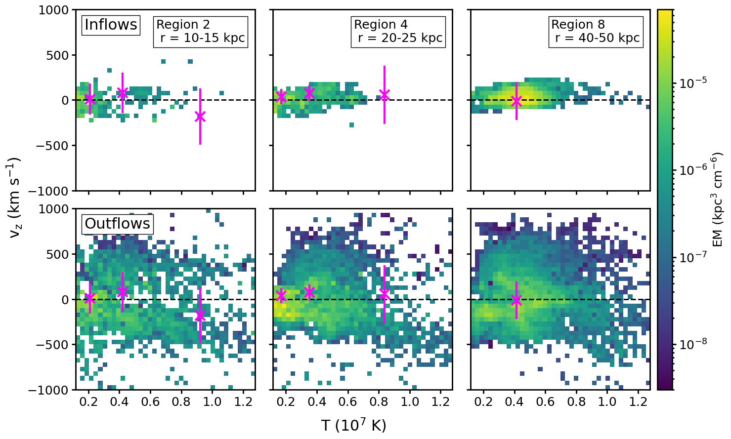
To further examine the consistency of the fitted values with the data from the simulation, we show in Figure 20 the phase space of temperature vs. line-of-sight velocity for 3 of the cylindrical annuli corresponding to the numbered face-on regions shown in the right panel of Figure 16. The top panels only show gas which is inflowing with $v_{r}<0$ and the bottom panels only show gas which is outflowing with $v_{r}>0$ (see also Section 3.2.1). The colormap indicates summed emission measure at each point, with yellow indicating the highest values. For each region, the general trend is for the phase space to be most concentrated at temperatures of $T\sim 3-6\times 10^{6}$ K ( $\sim 0.25-0.5$ keV), where the spread of velocities is also the lowest. As we move to higher temperatures, the spread of velocities increases, though the phase space is less populated in these regions.

Overplotted on each phase space panel are magenta points indicating the position of the fitted temperature and mean velocity from the bapec components shown in Figure 18, whereas the vertical error bars on each point indicate the velocity dispersion. For all of the panels, the coldest magenta point (Component 1 from Figure 18) is usually consistent with the highest emission measures in the region. We can also see from the top row of panels that this component is also consistent with inflowing gas, especially Region 8, which is at large radius and the gas with the highest emission measure should be near the disk and thus inflowing. However, there is also outflowing gas in these regions in projection (bottom row of panels) at the same velocity/temperature phase, so the distinction is not always clear-cut. Where present, Components 2 and 3 also appear generally consistent with the data, though once again there are larger uncertainties. These temperatures, especially Component 3, are hotter and are more consistent with the outflowing gas. This particular analysis relied on combinations of single temperature models, but it is likely that better models accounting for the temperature and velocity distributions in a more general way will need to be developed to properly model calorimeter-quality data in the future.

4 Summary

The hot, X-ray-emitting phase of the CGM has so far eluded detailed study, even for nearby galaxies, due to the brightness of the MW’s own CGM and the lack of X-ray instruments with sufficient spectral resolution to distinguish between the emission lines of the latter and the former. In disk galaxies with mass greater than or equal to the MW, the hot phase will be dominant. In the coming decades, determining the properties of this phase of the CGM will be crucial to the further development of our understanding the processes of galaxy formation and evolution. If our own galaxy is any indication, many of these galaxies may be expected to possess hot outflows (such as evidenced by the cavities seen in the eROSITA all-sky survey) and rotational motions in their CGM. Only X-ray IFUs will be able to map the velocity field of these galaxies to observe these processes in action.

Using a small selection of disk galaxies from the TNG50 simulation which were already shown to have cavities, we have shown that the CGM of such galaxies can exhibit velocities representing gas outflows, inflows, and rotation that can be mapped by microcalorimeter instruments of the future. Our main conclusions are as follows:

•

A number of the TNG50 galaxies examined in this sample (1-4) have a simple geometrical structure in the hot phase of the CGM, comprised of oppositely directed hot and fast outflows in conical regions on either side of the disk, coherent rotation in the inner hot CGM (within $\sim$ 50 kpc), and slower inflows of hot gas ( $\sim 100-150$ km s^-1) close to the galactic plane at larger radii. When viewed exactly edge-on, line shift maps exhibit the rotation curve clearly, with velocities of $\sim 100-200$ km s^-1. Hot outflows can also be seen edge-on in line shift ( $\sim 400-600$ km s^-1) if they are not launched exactly in the plane of the sky, and the expansion of the outflow along the sight line can be seen in line broadening measurements ( $\sim 200-400$ km s^-1). When viewed exactly face-on, line shift maps of the hot CGM of the same galaxies show a turbulent line-of-sight velocity structure with mean velocities of $\sim\pm 200-500$ km s^-1, and velocity dispersions of $\sim 300-1000$ km s^-1 within $\sim$ 50-100 kpc of the galactic center, and $\sim$ 100-200 km s^-1 at larger radii.
•

The hot CGM of these galaxies rotates in the same direction as the stellar disk and has a similar rotation speed ( $\sim 100-200$ km s^-1), but is slower than the colder CGM and ISM ( $\sim 200-400$ km s^-1). Conversely, the velocity dispersion in the azimuthal direction of the hot phase is greater ( $\sigma_{\phi}\sim$ 100-150 km s^-1) than the warm/cold phase ( $\sigma_{\phi}\sim$ 50-100 km s^-1). Outside of the rotation and outflow regions and closer to the disk, both phases of gas are inflowing, the hot phase at $\sim 100-150$ km s^-1 and the warm/cold phase at $\sim 100-300$ km s^-1.
•

If viewed face-on, the mean line-of-sight velocity in these galaxies azimuthally averages out to zero (assuming as we did in this work that the velocities are measured with respect to the center-of-mass frame). The velocity dispersion in this direction averages out to $\sigma\sim 200-500$ km s^-1 within $\sim$ 50-100 kpc and $\sigma\sim 100-200$ km s^-1 at larger radii. This structure is indicative of a complex pattern of flows that nevertheless when averaged over the azimuthal direction is composed of conically-shaped outflows away from the disk near the center and inflows at larger projected radii. We find that the velocity dispersion that is obtained is sensitive to which emission lines are used, since these probe different gas phases from each other and from the mass-weighted average.
•

Not all of the TNG galaxies we investigated display coherent rotation or inflow patterns in the hot CGM (in particular galaxies 5 and 6). These galaxies appear to have strong outflows not entirely aligned with the rotation axis of the stellar disk that may have disrupted the rotation and inflow of the hot CGM. These two galaxies are also the lowest-mass galaxies in our sample, and thus have less CGM gas in the hot phase which is more easily disrupted by feedback processes. Determining the precise reasons for the differences in the CGM velocity structure of these galaxies will require future work.
•

For X-ray observations, using regions larger than the angular resolution of the detector will often be necessary to obtain sufficient counts to measure the line centroid shift and broadening. This will not only measure velocity differences along the sight line, but also across the sky plane within the region, which also contributes to the measured centroid shift and broadening. We find that these contributions can be as significant to the overall measurement. To separate out these effects, splitting up the regions as finely as count rate statistics allow may be necessary.
•

When our galaxies are viewed at an angle inclined away from the disk, signs of both rotation and hot outflows are observed, the latter of which will be especially prominent in line shift measurements ( $\sim\pm 200-500$ km s^-1) in regions of X-ray SB which show evidence of cavities and bubbles. The combination of these effects produce a velocity pattern in our simulated galaxies that is distinct from the stellar and ISM velocity patterns, as the velocity fields of the latter two are dominated by rotation.
•

We produced mock X-ray microcalorimeter observations of galaxy 2 and used a spectral fitting technique to produce maps of the mean velocity field along two sight lines; edge-on and tilted 45^∘ to the rotation axis of the stellar disk. In both cases we are able to reproduce the features of the mean velocity field of the simulation to high-accuracy, enabling us to determine the properties of the rotation curve and the hot outflows.
•

We produced similar mock observations of galaxy 1 along the edge-on and face-on sightlines. We then selected regions in each projection to measure the first two moments of the velocity field by extracting spectra from these regions and fitting thermal emission models to them. We find that in the edge-on projection that the mean and standard deviation of the velocity are well-fit by a single thermal emission model, enabling us to measure the rotation curve of the CGM from line shifts and estimate the inflow velocity using line widths. In the face-on projection, the different phases of the gas have different velocities, and thus we require multiple thermal emission components to reproduce their properties. We find that the lower-temperature hot phase is consistent with lower velocity dispersions, and the higher-temperature gas is consistent with higher velocity dispersions. The former may be consistent with inflows (especially at large projected radii), whereas the latter is consistent with outflows, but projection effects make unambiguous identification of these two different phases difficult.

Our results show that future microcalorimeter observations of the hot CGM of galaxies will be able to measure the temperature and velocity fields of the gas, and determine if the hot CGM has the main structures we identified in this work: inflows, outflows, and rotation, or if is dominated by a chaotic and turbulent flow like two of the galaxies in our sample. Detecting hot outflows and measuring their velocities will help determine the mass and energy fluxes of these outflows, and thus their impact on the evolution of the galaxy and its environment. Measuring the rotation and inflow velocities of the hot CGM, especially in comparison to measurements of the cooler phase in the UV, will help determine how gas accretes from the CGM onto the galaxy itself in its different temperature phases and drives its evolution.

This analysis could be extended in a number of ways. The spectral analysis of the mock observations in this work merely scratched the surface of what is possible. The closest analog to studies of the hot halos of galaxies are their more massive counterparts in groups and clusters of galaxies in the intragroup and intracluster media. These are much brighter in X-rays and hence easier to study. In the era of Chandra, XMM-Newton, Suzaku, NuSTAR, and now eROSITA, spectral analysis of these extended sources has been largely limited to the $\sim$ 100 eV resolution of the imaging instruments on these telescopes. This prevents analysis of the velocity field in groups and clusters, and limits the ability to distinguish between different gas phases of different temperatures and compositions. This latter issue has not been a major limitation for most studies of the hot gas in groups and clusters, since for most applications it is well-approximated by a single-temperature phase over relevant spatial regions. However, this is not the case for the CGM, and to characterize it adequately we will need microcalorimeter instruments that can resolve the velocity field and the different gas phases. Extensions of the work presented here should focus on improvements to the process of extracting and fitting spectra to decompose the emission into these multiple thermodynamic and kinematic components, which will likely require more sophisticated statistical methods than have been required for spectra with CCD-like energy resolution, and/or machine learning techniques.

We have also only used disk galaxies from the TNG simulations, which prescribe particular modes of AGN and stellar feedback. It would be instructive to perform similar analyses on other simulated galaxies, including from cosmological simulations such as EAGLE (Schaye et al., 2015; Crain et al., 2015), SIMBA (Davé et al., 2019), FIRE (Hopkins et al., 2018, 2023), Magneticum (Biffi et al., 2013), ChaNGa (Sanchez et al., 2019), and FOGGIE (Peeples et al., 2019), or idealized simulations (Fielding et al., 2017; Schneider & Robertson, 2018; Stern et al., 2023).

JAZ, AB, PEJN, and RPK are funded by the Chandra X-ray Center, which is operated by the Smithsonian Astrophysical Observatory for and on behalf of NASA under contract NAS8-03060. JS was supported by the Israel Science Foundation (grant No. 2584/21). DN acknowledges funding from the Deutsche Forschungsgemeinschaft (DFG) through an Emmy Noether Research Group (grant number NE 2441/1-1). IK acknowledges support by the COMPLEX project from the European Research Council (ERC) under the European Union’s Horizon 2020 research and innovation program grant agreement ERC-2019-AdG 882679. This material is based upon work supported by NASA under award number 80GSFC21M0002. The TNG50 simulation was run with compute time granted by the Gauss Centre for Supercomputing (GCS) under Large-Scale Projects GCS-DWAR on the GCS share of the supercomputer Hazel Hen at the High Performance Computing Center Stuttgart (HLRS).

References

Anders & Grevesse (1989) Anders, E., & Grevesse, N. 1989, Geochim. Cosmochim. Acta, 53, 197, doi: 10.1016/0016-7037(89)90286-X
Anderson & Bregman (2011) Anderson, M. E., & Bregman, J. N. 2011, ApJ, 737, 22, doi: 10.1088/0004-637X/737/1/22
Anderson et al. (2013) Anderson, M. E., Bregman, J. N., & Dai, X. 2013, ApJ, 762, 106, doi: 10.1088/0004-637X/762/2/106
Anderson et al. (2015) Anderson, M. E., Gaspari, M., White, S. D. M., Wang, W., & Dai, X. 2015, MNRAS, 449, 3806, doi: 10.1093/mnras/stv437
Arnaud (1996) Arnaud, K. A. 1996, in Astronomical Society of the Pacific Conference Series, Vol. 101, Astronomical Data Analysis Software and Systems V, ed. G. H. Jacoby & J. Barnes, 17
Astropy Collaboration et al. (2013) Astropy Collaboration, Robitaille, T. P., Tollerud, E. J., et al. 2013, A&A, 558, A33, doi: 10.1051/0004-6361/201322068
Astropy Collaboration et al. (2018) Astropy Collaboration, Price-Whelan, A. M., Sipőcz, B. M., et al. 2018, AJ, 156, 123, doi: 10.3847/1538-3881/aabc4f
Bandler et al. (2019) Bandler, S. R., Chervenak, J. A., Datesman, A. M., et al. 2019, Journal of Astronomical Telescopes, Instruments, and Systems, 5, 021017, doi: 10.1117/1.JATIS.5.2.021017
Barret et al. (2016) Barret, D., Lam Trong, T., den Herder, J.-W., et al. 2016, in Society of Photo-Optical Instrumentation Engineers (SPIE) Conference Series, Vol. 9905, Space Telescopes and Instrumentation 2016: Ultraviolet to Gamma Ray, ed. J.-W. A. den Herder, T. Takahashi, & M. Bautz, 99052F, doi: 10.1117/12.2232432
Barret et al. (2018) Barret, D., Lam Trong, T., den Herder, J.-W., et al. 2018, in Society of Photo-Optical Instrumentation Engineers (SPIE) Conference Series, Vol. 10699, Space Telescopes and Instrumentation 2018: Ultraviolet to Gamma Ray, ed. J.-W. A. den Herder, S. Nikzad, & K. Nakazawa, 106991G, doi: 10.1117/12.2312409
Bertone et al. (2013) Bertone, S., Aguirre, A., & Schaye, J. 2013, MNRAS, 430, 3292, doi: 10.1093/mnras/stt131
Biffi et al. (2013) Biffi, V., Dolag, K., & Böhringer, H. 2013, MNRAS, 428, 1395, doi: 10.1093/mnras/sts120
Bluem et al. (2022) Bluem, J., Kaaret, P., Kuntz, K. D., et al. 2022, ApJ, 936, 72, doi: 10.3847/1538-4357/ac8662
Bogdán et al. (2017) Bogdán, Á., Bourdin, H., Forman, W. R., et al. 2017, ApJ, 850, 98, doi: 10.3847/1538-4357/aa9523
Bogdán et al. (2013) Bogdán, Á., Forman, W. R., Kraft, R. P., & Jones, C. 2013, ApJ, 772, 98, doi: 10.1088/0004-637X/772/2/98
Bogdan et al. (2023) Bogdan, A., Khabibullin, I., Kovacs, O., et al. 2023, arXiv e-prints, arXiv:2306.05449, doi: 10.48550/arXiv.2306.05449
Bordoloi et al. (2011) Bordoloi, R., Lilly, S. J., Knobel, C., et al. 2011, ApJ, 743, 10, doi: 10.1088/0004-637X/743/1/10
Bordoloi et al. (2014) Bordoloi, R., Tumlinson, J., Werk, J. K., et al. 2014, ApJ, 796, 136, doi: 10.1088/0004-637X/796/2/136
Burchett et al. (2021) Burchett, J. N., Rubin, K. H. R., Prochaska, J. X., et al. 2021, ApJ, 909, 151, doi: 10.3847/1538-4357/abd4e0
Burchett et al. (2016) Burchett, J. N., Tripp, T. M., Bordoloi, R., et al. 2016, ApJ, 832, 124
Burchett et al. (2019) Burchett, J. N., Tripp, T. M., Prochaska, J. X., et al. 2019, ApJ, 877, L20, doi: 10.3847/2041-8213/ab1f7f
Burke et al. (2020) Burke, D., Laurino, O., Wmclaugh, et al. 2020, sherpa/sherpa: Sherpa 4.12.1, 4.12.1, Zenodo, Zenodo, doi: 10.5281/zenodo.3944985
Cash (1979) Cash, W. 1979, ApJ, 228, 939, doi: 10.1086/156922
Chadayammuri et al. (2022) Chadayammuri, U., Bogdán, Á., Oppenheimer, B. D., et al. 2022, ApJ, 936, L15, doi: 10.3847/2041-8213/ac8936
Churchill et al. (2013) Churchill, C. W., Trujillo-Gomez, S., Nielsen, N. M., & Kacprzak, G. G. 2013, ApJ, 779, 87, doi: 10.1088/0004-637X/779/1/87
Comparat et al. (2022) Comparat, J., Truong, N., Merloni, A., et al. 2022, A&A, 666, A156, doi: 10.1051/0004-6361/202243101
Crain et al. (2015) Crain, R. A., Schaye, J., Bower, R. G., et al. 2015, MNRAS, 450, 1937, doi: 10.1093/mnras/stv725
Cui et al. (2020) Cui, W., Bregman, J. N., Bruijn, M. P., et al. 2020, in Society of Photo-Optical Instrumentation Engineers (SPIE) Conference Series, Vol. 11444, Space Telescopes and Instrumentation 2020: Ultraviolet to Gamma Ray, ed. J.-W. A. den Herder, S. Nikzad, & K. Nakazawa, 114442S, doi: 10.1117/12.2560871
Das et al. (2020) Das, S., Mathur, S., & Gupta, A. 2020, ApJ, 897, 63, doi: 10.3847/1538-4357/ab93d2
Das et al. (2019) Das, S., Mathur, S., Gupta, A., et al. 2019, ApJ, 885, 108, doi: 10.3847/1538-4357/ab48df
Davé et al. (2019) Davé, R., Anglés-Alcázar, D., Narayanan, D., et al. 2019, MNRAS, 486, 2827, doi: 10.1093/mnras/stz937
DeFelippis et al. (2020) DeFelippis, D., Genel, S., Bryan, G. L., et al. 2020, ApJ, 895, 17, doi: 10.3847/1538-4357/ab8a4a
Fielding et al. (2017) Fielding, D., Quataert, E., McCourt, M., & Thompson, T. A. 2017, MNRAS, 466, 3810, doi: 10.1093/mnras/stw3326
Foreman-Mackey et al. (2013) Foreman-Mackey, D., Hogg, D. W., Lang, D., & Goodman, J. 2013, PASP, 125, 306, doi: 10.1086/670067
Freeman et al. (2002) Freeman, P. E., Kashyap, V., Rosner, R., & Lamb, D. Q. 2002, ApJS, 138, 185, doi: 10.1086/324017
Fruscione et al. (2006) Fruscione, A., McDowell, J. C., Allen, G. E., et al. 2006, in Society of Photo-Optical Instrumentation Engineers (SPIE) Conference Series, Vol. 6270, Observatory Operations: Strategies, Processes, and Systems, ed. D. R. Silva & R. E. Doxsey, 62701V, doi: 10.1117/12.671760
Hafen et al. (2022) Hafen, Z., Stern, J., Bullock, J., et al. 2022, MNRAS, 514, 5056, doi: 10.1093/mnras/stac1603
Harris et al. (2020) Harris, C. R., Millman, K. J., van der Walt, S. J., et al. 2020, Nature, 585, 357, doi: 10.1038/s41586-020-2649-2
Hitomi Collaboration et al. (2016) Hitomi Collaboration, Aharonian, F., Akamatsu, H., et al. 2016, Nature, 535, 117, doi: 10.1038/nature18627
Hitomi Collaboration et al. (2017) —. 2017, Nature, 551, 478, doi: 10.1038/nature24301
Hitomi Collaboration et al. (2018a) —. 2018a, PASJ, 70, 9, doi: 10.1093/pasj/psx138
Hitomi Collaboration et al. (2018b) —. 2018b, PASJ, 70, 10, doi: 10.1093/pasj/psx127
Hitomi Collaboration et al. (2018c) —. 2018c, PASJ, 70, 10, doi: 10.1093/pasj/psx127
Hitomi Collaboration et al. (2018d) —. 2018d, PASJ, 70, 12, doi: 10.1093/pasj/psx156
Hodges-Kluck et al. (2016) Hodges-Kluck, E. J., Miller, M. J., & Bregman, J. N. 2016, ApJ, 822, 21, doi: 10.3847/0004-637X/822/1/21
Hopkins et al. (2018) Hopkins, P. F., Wetzel, A., Kereš, D., et al. 2018, MNRAS, 480, 800, doi: 10.1093/mnras/sty1690
Hopkins et al. (2023) Hopkins, P. F., Wetzel, A., Wheeler, C., et al. 2023, MNRAS, 519, 3154, doi: 10.1093/mnras/stac3489
Humphrey et al. (2011) Humphrey, P. J., Buote, D. A., Canizares, C. R., Fabian, A. C., & Miller, J. M. 2011, ApJ, 729, 53, doi: 10.1088/0004-637X/729/1/53
Hunter (2007) Hunter, J. D. 2007, Computing in Science & Engineering, 9, 90, doi: 10.1109/MCSE.2007.55
Huscher et al. (2021) Huscher, E., Oppenheimer, B. D., Lonardi, A., et al. 2021, MNRAS, 500, 1476, doi: 10.1093/mnras/staa3203
Johnson et al. (2015) Johnson, S. D., Chen, H.-W., & Mulchaey, J. S. 2015, MNRAS, 449, 3263, doi: 10.1093/mnras/stv553
Kraft et al. (2023) Kraft, R., Markevitch, M., Kilbourne, C., et al. 2023, Line Emission Mapper (LEM): Probing the physics of cosmic ecosystems. https://arxiv.org/abs/2211.09827
Kuntz (2019) Kuntz, K. D. 2019, A&A Rev., 27, 1, doi: 10.1007/s00159-018-0114-0
Lehmer et al. (2012) Lehmer, B. D., Xue, Y. Q., Brandt, W. N., et al. 2012, ApJ, 752, 46, doi: 10.1088/0004-637X/752/1/46
Li et al. (2018) Li, J.-T., Bregman, J. N., Wang, Q. D., Crain, R. A., & Anderson, M. E. 2018, ApJ, 855, L24, doi: 10.3847/2041-8213/aab2af
Li et al. (2017) Li, J.-T., Bregman, J. N., Wang, Q. D., et al. 2017, ApJS, 233, 20, doi: 10.3847/1538-4365/aa96fc
McCammon et al. (2002) McCammon, D., Almy, R., Apodaca, E., et al. 2002, ApJ, 576, 188, doi: 10.1086/341727
Nelson et al. (2019a) Nelson, D., Pillepich, A., Springel, V., et al. 2019a, MNRAS, 490, 3234, doi: 10.1093/mnras/stz2306
Nelson et al. (2019b) Nelson, D., Springel, V., Pillepich, A., et al. 2019b, Computational Astrophysics and Cosmology, 6, 2, doi: 10.1186/s40668-019-0028-x
Nelson et al. (2023) Nelson, D., Byrohl, C., Ogorzalek, A., et al. 2023, MNRAS, 522, 3665, doi: 10.1093/mnras/stad1195
Nica et al. (2022) Nica, A., Oppenheimer, B. D., Crain, R. A., et al. 2022, MNRAS, 517, 1958, doi: 10.1093/mnras/stac2020
Nielsen et al. (2013) Nielsen, N. M., Churchill, C. W., Kacprzak, G. G., & Murphy, M. T. 2013, ApJ, 776, 114, doi: 10.1088/0004-637X/776/2/114
Oppenheimer (2018) Oppenheimer, B. D. 2018, MNRAS, 480, 2963, doi: 10.1093/mnras/sty1918
Pakmor & Springel (2013) Pakmor, R., & Springel, V. 2013, MNRAS, 432, 176, doi: 10.1093/mnras/stt428
Peeples et al. (2014) Peeples, M. S., Werk, J. K., Tumlinson, J., et al. 2014, ApJ, 786, 54, doi: 10.1088/0004-637X/786/1/54
Peeples et al. (2019) Peeples, M. S., Corlies, L., Tumlinson, J., et al. 2019, ApJ, 873, 129, doi: 10.3847/1538-4357/ab0654
Pillepich et al. (2021) Pillepich, A., Nelson, D., Truong, N., et al. 2021, MNRAS, 508, 4667, doi: 10.1093/mnras/stab2779
Pillepich et al. (2018) Pillepich, A., Springel, V., Nelson, D., et al. 2018, MNRAS, 473, 4077, doi: 10.1093/mnras/stx2656
Pillepich et al. (2019) Pillepich, A., Nelson, D., Springel, V., et al. 2019, MNRAS, 490, 3196, doi: 10.1093/mnras/stz2338
Planck Collaboration et al. (2016) Planck Collaboration, Ade, P. A. R., Aghanim, N., et al. 2016, A&A, 594, A13, doi: 10.1051/0004-6361/201525830
Ponti et al. (2022) Ponti, G., Zheng, X., Locatelli, N., et al. 2022, arXiv e-prints, arXiv:2210.03133, doi: 10.48550/arXiv.2210.03133
Price-Whelan & Foreman-Mackey (2017) Price-Whelan, A. M., & Foreman-Mackey, D. 2017, The Journal of Open Source Software, 2, doi: 10.21105/joss.00357
Prochaska et al. (2017) Prochaska, J. X., Werk, J. K., Worseck, G., et al. 2017, ApJ, 837, 169, doi: 10.3847/1538-4357/aa6007
Ramesh et al. (2023a) Ramesh, R., Nelson, D., & Pillepich, A. 2023a, MNRAS, 518, 5754, doi: 10.1093/mnras/stac3524
Ramesh et al. (2023b) —. 2023b, MNRAS, 522, 1535, doi: 10.1093/mnras/stad951
Rupke et al. (2019) Rupke, D. S. N., Coil, A., Geach, J. E., et al. 2019, Nature, 574, 643, doi: 10.1038/s41586-019-1686-1
Sanchez et al. (2019) Sanchez, N. N., Werk, J. K., Tremmel, M., et al. 2019, ApJ, 882, 8, doi: 10.3847/1538-4357/ab3045
Schaye et al. (2015) Schaye, J., Crain, R. A., Bower, R. G., et al. 2015, MNRAS, 446, 521, doi: 10.1093/mnras/stu2058
Schneider & Robertson (2018) Schneider, E. E., & Robertson, B. E. 2018, ApJ, 860, 135, doi: 10.3847/1538-4357/aac329
Smith et al. (2001) Smith, R. K., Brickhouse, N. S., Liedahl, D. A., & Raymond, J. C. 2001, ApJ, 556, L91, doi: 10.1086/322992
Sormani et al. (2018) Sormani, M. C., Sobacchi, E., Pezzulli, G., Binney, J., & Klessen, R. S. 2018, MNRAS, 481, 3370, doi: 10.1093/mnras/sty2500
Springel (2010) Springel, V. 2010, MNRAS, 401, 791, doi: 10.1111/j.1365-2966.2009.15715.x
Stern et al. (2020) Stern, J., Fielding, D., Faucher-Giguère, C.-A., & Quataert, E. 2020, MNRAS, 492, 6042, doi: 10.1093/mnras/staa198
Stern et al. (2023) Stern, J., Fielding, D., Hafen, Z., et al. 2023, arXiv e-prints, arXiv:2306.00092, doi: 10.48550/arXiv.2306.00092
Stewart et al. (2017) Stewart, K. R., Maller, A. H., Oñorbe, J., et al. 2017, ApJ, 843, 47, doi: 10.3847/1538-4357/aa6dff
Stocke et al. (2013) Stocke, J. T., Keeney, B. A., Danforth, C. W., et al. 2013, ApJ, 763, 148, doi: 10.1088/0004-637X/763/2/148
Truong et al. (2021) Truong, N., Pillepich, A., Nelson, D., Werner, N., & Hernquist, L. 2021, MNRAS, 508, 1563, doi: 10.1093/mnras/stab2638
Tumlinson et al. (2017) Tumlinson, J., Peeples, M. S., & Werk, J. K. 2017, ARA&A, 55, 389, doi: 10.1146/annurev-astro-091916-055240
Tumlinson et al. (2011) Tumlinson, J., Thom, C., Werk, J. K., et al. 2011, Science, 334, 948, doi: 10.1126/science.1209840
Tumlinson et al. (2013) —. 2013, ApJ, 777, 59, doi: 10.1088/0004-637X/777/1/59
Turk et al. (2011) Turk, M. J., Smith, B. D., Oishi, J. S., et al. 2011, ApJS, 192, 9, doi: 10.1088/0067-0049/192/1/9
Vogelsberger et al. (2020) Vogelsberger, M., Marinacci, F., Torrey, P., & Puchwein, E. 2020, Nature Reviews Physics, 2, 42, doi: 10.1038/s42254-019-0127-2
Vogelsberger et al. (2014a) Vogelsberger, M., Genel, S., Springel, V., et al. 2014a, Nature, 509, 177, doi: 10.1038/nature13316
Vogelsberger et al. (2014b) —. 2014b, MNRAS, 444, 1518, doi: 10.1093/mnras/stu1536
Weinberger et al. (2017) Weinberger, R., Springel, V., Hernquist, L., et al. 2017, MNRAS, 465, 3291, doi: 10.1093/mnras/stw2944
Werk et al. (2013) Werk, J. K., Prochaska, J. X., Thom, C., et al. 2013, ApJS, 204, 17
Werk et al. (2014) Werk, J. K., Prochaska, J. X., Tumlinson, J., et al. 2014, ApJ, 792, 8, doi: 10.1088/0004-637X/792/1/8
Werk et al. (2016) Werk, J. K., Prochaska, J. X., Cantalupo, S., et al. 2016, ApJ, 833, 54, doi: 10.3847/1538-4357/833/1/54
Wilms et al. (2000) Wilms, J., Allen, A., & McCray, R. 2000, ApJ, 542, 914, doi: 10.1086/317016
XRISM Science Team (2020) XRISM Science Team. 2020, arXiv e-prints, arXiv:2003.04962, doi: 10.48550/arXiv.2003.04962
ZuHone & Hallman (2016) ZuHone, J. A., & Hallman, E. J. 2016, pyXSIM: Synthetic X-ray observations generator, Astrophysics Source Code Library, record ascl:1608.002. http://ascl.net/1608.002
ZuHone et al. (2016) ZuHone, J. A., Miller, E. D., Simionescu, A., & Bautz, M. W. 2016, ApJ, 821, 6, doi: 10.3847/0004-637X/821/1/6
ZuHone et al. (2023) ZuHone, J. A., Vikhlinin, A., Tremblay, G. R., et al. 2023, SOXS: Simulated Observations of X-ray Sources, Astrophysics Source Code Library, record ascl:2301.024. http://ascl.net/2301.024

Appendix A Plots for Galaxies 3, 4, and 5

This appendix shows the main figures for galaxies 3, 4, and 5, mentioned previously in Section 3. These galaxies are lower-mass and not as bright in X-rays as galaxies 1 and 2 (though galaxy 6 is the lowest-mass galaxy in our sample). In general, galaxies 3 and 4 are very similar to 1 and 2 in the sense that they have the same general pattern of inflows, outflows, and rotation. Galaxy 5 is similar to galaxy 6 in the sense that it has an outflow that is not symmetric on either side of the disk and its velocity field appears more turbulent.