Mapping the imprints of stellar and AGN feedback in the circumgalactic medium with X-ray microcalorimeters

Abstract

The Astro2020 Decadal Survey has identified the mapping of the circumgalactic medium (CGM, gaseous plasma around galaxies) as a key objective. We explore the prospects for characterizing the CGM in and around nearby galaxy halos with future large grasp X-ray microcalorimeters. We create realistic mock observations from hydrodynamical simulations (EAGLE, IllustrisTNG, and Simba) that demonstrate a wide range of potential measurements, which will address the open questions in galaxy formation and evolution. By including all background and foreground components in our mock observations, we show why it is impossible to perform these measurements with current instruments, such as X-ray CCDs, and only microcalorimeters will allow us to distinguish the faint CGM emission from the bright Milky Way (MW) foreground emission lines.

We find that individual halos of MW mass can, on average, be traced out to large radii, around R₅₀₀, and for larger galaxies even out to R₂₀₀, using the O VII, O VIII, or Fe XVII emission lines. Furthermore, we show that emission line ratios for individual halos can reveal the radial temperature structure. Substructure measurements show that it will be possible to relate azimuthal variations to the feedback mode of the galaxy. We demonstrate the ability to construct temperature, velocity, and abundance ratio maps from spectral fitting for individual galaxy halos, which reveal rotation features, AGN outbursts, and enrichment.

tablenum SIXtablenum

1 Introduction

Structure formation models predict that galaxies reside in massive dark matter halos and are embedded in large-scale gaseous halos, the circumgalactic medium (CGM). The CGM plays a crucial role in the evolution of galaxies as gas flows through the CGM and regulates galaxy growth over cosmic time. To establish a comprehensive picture of the formation and evolution of galaxies, it is essential to probe the interplay between the stellar body, the supermassive black hole (SMBH), and the large-scale CGM. While the stellar component and SMBHs of galaxies have been the subject of a wide range of studies over the past decades, our knowledge about the CGM remains very limited, which poses major gaps in our understanding of galaxy formation and evolution. The importance of the CGM is highlighted by the fact that it plays a role on a wide range of spatial scales from small-scale processes (e.g. galactic winds driven by supernovae) to the largest scales of galaxies (e.g. accretion of gas from large scale structure filaments).

Theoretical and observational studies hint that the CGM has a complex and multi-phase structure. In Milky Way-type and more massive galaxies, the dominant phases of the CGM have characteristic temperatures of millions of degrees and are predominantly observable at X-ray wavelengths (e.g., Crain et al., 2010; van de Voort & Schaye, 2013; Nelson et al., 2018a; Wijers & Schaye, 2022). Indeed, in the well-established picture of structure formation, dark matter halos accrete baryonic matter, which is thermalized in an accretion shock (White & Rees, 1978; White & Frenk, 1991). The characteristic temperature is determined by the gravitational potential of the galaxies and reaches X-ray temperatures ($\gtrsim 10^{6}$ K) for Milky Way-type galaxies. Since the cooling time of the hot gas is much longer than the dynamical time, the CGM is expected to be quasi-static and should be observable around galaxies in the present-day universe.

Because the importance of studying the X-ray emitting large-scale gaseous component of galaxies was recognized decades ago, all major X-ray observatories attempted to explore this component. Studies of elliptical (or quiescent) galaxies achieved significant success in the early days of X-ray astronomy (Nulsen et al., 1984; O’Sullivan et al., 2001). Observations of massive ellipticals with the Einstein and ROSAT observatories revealed the presence of gaseous X-ray halos that extend beyond the optical extent of galaxies (Forman et al., 1985; Trinchieri & Fabbiano, 1985; Mathews, 1990; Mathews & Brighenti, 2003). These observations not only revealed the ubiquity of the gaseous halos, but allowed characterizations of the physical properties of the X-ray gas, and measurements of its mass within various radii. Follow-up observations with XMM-Newton and Chandra played a major role in further probing the gaseous emission around a larger sample of nearby massive elliptical galaxies (Anderson & Bregman, 2011; Bogdán et al., 2013a, 2015; Goulding et al., 2016; Bogdán et al., 2017; Li et al., 2018). Thanks to the sub-arcsecond angular resolution of Chandra, it became possible to clearly resolve and separate point-like sources, such as low-mass X-ray binaries and AGN, from the truly diffuse gaseous emission (Bogdán & Gilfanov, 2011). This allowed more detailed studies of the X-ray-emitting interstellar medium and the larger-scale CGM. However, a major hindrance to studying elliptical galaxies is that the dominant fraction of galaxies explored by Chandra and XMM-Newton reside in rich environments, such as galaxy groups or galaxy clusters. The presence of these group and cluster atmospheres makes it virtually impossible to differentiate the CGM component of the galaxy from the large-scale group or cluster emission. Because the group or cluster atmosphere will dominate the overall emission beyond the optical radius, it becomes impossible to separate these components from each other and determine their relative contributions. Additionally, the gaseous component around quiescent galaxies is likely a mix of the infalling primordial gas onto the dark matter halos and the ejected gas from evolved stars, which was shock heated to the kinetic temperature of the galaxy. Due to quenching mechanisms, most quiescent galaxies reside in galaxy groups and clusters, which are not ideal targets to probe the primordial gas.

As opposed to their quiescent counterparts, star-forming galaxies provide the ideal framework to probe the gas originating from the primordial infall. The main advantage of disk (or star-forming) galaxies is their environment. While quiescent galaxies form through mergers, which happen at a higher likelihood in rich environments, due to the higher galaxy density, a substantial fraction of star-forming galaxies will preferentially reside in relatively isolated environments. The CGM around disk galaxies was also probed in a wide range of observations. Using ROSAT observations, the X-ray gas around disk galaxies remained undetected (Benson et al., 2000). However, this posed a challenge to galaxy formation models that predicted bright enough gaseous halos to be observed around nearby disk galaxies (White & Frenk, 1991; Crain et al., 2010; Vogelsberger et al., 2020). Revising these models and involving efficient feedback from AGN drastically decreased the predicted X-ray luminosity of the X-ray CGM, implying that non-detection by ROSAT was consistent with theoretical models. More sensitive observations with Chandra and XMM-Newton led to the detection of the CGM around isolated massive disk galaxies (e.g., Wang et al., 2001; Li et al., 2006, 2007; Crain et al., 2010). Most notably, the CGM of two massive galaxies, NGC 1961 and NGC 6753, was detected and characterized out to about $50-60$ kpc radius, which corresponds to about $0.15r_{\rm 200}$, where $r_{\rm 200}$ is the radius within which the density is 200 times the critical density of the Universe, and we consider it to be the virial radius of the galaxies. These studies not only detected the gas, but also measured the basic properties of the CGM, such as the temperature and abundance, and established simple thermodynamic profiles (Anderson & Bregman, 2011; Bogdán et al., 2013a; Anderson et al., 2015; Bogdán et al., 2017). Following these detections, the CGM of other disk galaxies was also explored albeit to a much lesser extent due to the lower signal-to-noise ratios of these galaxies (Dai et al., 2012; Bogdán et al., 2013b; Li et al., 2017). Despite these successes, however, it is important to realize that all these detections explored massive galaxies (few $\times 10^{11}\ \rm{M_{\odot}}$ in stellar mass), while the CGM emission around Milky Way-type galaxies remains undetected.

The main challenge in detecting the extended CGM of external galaxies is due to the hot gas residing in our own Milky Way. Specifically, our Solar system is surrounded by the local hot bubble (LHB), which has a characteristic temperature of $kT\approx$0.1\text{\,}\mathrm{k}\mathrm{e}\mathrm{V}$$ (McCammon et al., 2002; Das et al., 2019a). On the larger scales, the Milky Way also hosts an extended hot component with a characteristic temperature of $\sim$0.2\text{\,}\mathrm{k}\mathrm{e}\mathrm{V}$$ (McCammon et al., 2002; Das et al., 2019a). These gas temperatures are comparable to those expected from other external galaxies and, since both the Milky Way and the other galaxies exhibit the same thermal emission component, the emission signal from the low-surface brightness CGM of external galaxies can be orders of magnitude below the Milky Way foreground emission. Because the X-ray emission from the Milky Way foreground is present in every sightline and this component cannot be differentiated at CCD resolution ($\sim 50-100$ eV), its contribution cannot be easily removed from the CGM component of other galaxies. A direct consequence of this is that even future telescopes with larger collecting areas with CCD-like instruments will be limited by the foreground emission and thus cannot probe the large-scale CGM. To achieve a transformative result in exploring the extended CGM, we must utilize high spectral resolution spectroscopy to spectroscopically differentiate the emission lines from the Milky Way foreground from those emitted by the external galaxies. We emphasize that mapping the CGM is essential in order to learn about its distribution, enrichment, and thermodynamic structure, which is not feasible with dispersive (grating) spectroscopy.

Recent advances in technology allow us to take this transformative step. The development of high spectral resolution X-ray Integral Field Units (IFUs) provides the much-needed edge over traditional CCD-like instruments. Notably, X-ray IFUs can simultaneously provide traditional images with good spatial resolution and very high, $1-2$ eV, spectral resolution across the array. In this work, we explore how utilizing the new technology of X-ray IFUs can drastically change our understanding of galaxy formation. We assume capabilities similar to the Line Emission Mapper (LEM) Probe mission concept (Kraft et al., 2022). The LEM concept is designed to have a large field-of-view ($\gtrsim$900\text{\,}\mathrm{a}\mathrm{r}\mathrm{c}\mathrm{m}\mathrm{i}\mathrm{n}^{2}$$), state-of-the-art X-ray microcalorimeter with 1 eV spectral resolution in the central array, and 2 eV spectral resolution across the field-of-view. The single-instrument telescope is planned to have $2500\text{\,}\mathrm{c}\mathrm{m}^{2}$ collecting area at $1\text{\,}\mathrm{k}\mathrm{e}\mathrm{V}$ energy. Overall, the spectral resolution of LEM surpasses that of CCD-like instruments by $50-100$ times, allowing us to spectrally separate the Milky Way foreground lines and the emission lines from the CGM of external galaxies.

Modern cosmological hydrodynamical simulations are able to model the detailed distribution of the hot CGM (e.g., Cen & Ostriker, 1999, 2000). The divergence among these simulations is chiefly driven by the difference in modelling baryonic physics, most notably the modelling of feedback processes, such as those driven by star formation activities or accretion onto SMBHs (see e.g. Vogelsberger et al., 2020 for a recent review). Intrinsic limitations due to the finite resolution of these simulations require sub-resolution models, which add uncertainties to the results. Sub-resolution feedback effects are implemented to mimic net effects of AGN feedback, but depend on the numerical implementation. The simulations of the IllustrisTNG project, for example, switch from thermal to kinetic feedback mode, depending on the chosen thresold of the AGN accretion rate (Weinberger et al., 2017; Vogelsberger et al., 2020). Other simulations, such as EAGLE, use only the thermal AGN feedback channel to reheat the gas (Schaye et al., 2015). Thus, simulations are significantly diverse in predicting the CGM properties (e.g., X-ray line emission profiles, see van de Voort & Schaye, 2013; Wijers & Schaye, 2022, Truong et al. 2023). Therefore, probing the hot phases of the CGM is essential to understand how feedback processes operate on galactic scales, and future observations will constrain models by comparison of observations with simulations.

In this work, we utilize three modern hydrodynamical structure formation simulations, IllustrisTNG, EAGLE, and Simba, to demonstrate that LEM will provide an unprecedented view into the formation and evolution of galaxies. In section 2 we describe the hydrodynamical simulations and the setup of the mock observations. We show the surface brightness profiles of 4 bright emission lines for galaxy subsamples selected by halo mass and star formation rate in section 3. We also quantify the level of substructure and present 2D maps of the temperature and element abundance ratios inferred from a spectral analysis. Section 4 discusses the results.

2 Methods

Here we describe our methodology for the analysis of microcalorimeter mock observations.

2.1 An X-ray Probe microcalorimeter with large grasp

There are currently several missions and mission concepts with a microcalorimeter, such as Athena X-IFU (Barret et al., 2013, 2018, 2023), the X-Ray Imaging and Spectroscopy Mission (XRISM, Terada et al., 2021), the Hot Universe Baryon Surveyor (HUBS, Zhang et al., 2022), and the Line Emission Mapper (LEM, Kraft et al., 2022). However, the CGM can be best probed by a large area, large field of view instrument (i.e., large grasp, which is the product of the field of view and collecting area), with the characteristics of LEM, a probe concept designed for the X-ray detection of the faint emission lines of the CGM with unprecedented spectral resolution. The spatial resolution (half-power diameter, HPD) of $10\text{\,}\arcsec$ will be utilized through a dithering pattern, similar to Chandra, and will allow the separation and exclusion of bright point sources to resolve the structure of the CGM. We assume a collecting area of $2500\text{\,}\mathrm{c}\mathrm{m}^{2}$ at $1\text{\,}\mathrm{k}\mathrm{e}\mathrm{V}$ ($1600\text{\,}\mathrm{c}\mathrm{m}^{2}$ at $0.5\text{\,}\mathrm{k}\mathrm{e}\mathrm{V}$) and a bandpass from 0.2 to 2 keV, which is ideal to map nearby galaxies (see Kraft et al., 2022). Through its large grasp and $12\text{\,}\mathrm{e}\mathrm{V}$ resolution, it is far superior to any other high spectral resolution instrument for surveying the CGM emission. We emphasize that the spectral resolution will at least provide the ability to disentangle the redshifted line emission, namely C VI, O VII, O VIII, Fe XVII, from the bright foreground line emission of our Milky Way, i.e. a few eV depending on the redshift.

Although the LEM concept includes a high-resolution (1 eV) central array, we only consider the energy resolution of the main array (2 eV), since the angular sizes of objects considered here exceed the FoV of the central array and require the full field of view. A galaxy with similar stellar mass as our Milky Way will reach about $R_{500}=$165\text{\,}\mathrm{k}\mathrm{p}\mathrm{c}$$, which corresponds to $13\text{\,}\mathrm{a}\mathrm{r}\mathrm{c}\mathrm{m}\mathrm{i}\mathrm{n}$ at $z=0.01$. Therefore, we conservatively only consider a 2 eV resolution throughout the field of view. For larger and brighter galaxies with about twice the Milky Way stellar mass at a slightly larger distance ($z=0.035$), we are able to trace the CGM even beyond $R_{500}$.

2.2 Mock observations of hydro-dynamical cosmological simulations

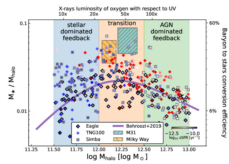
Figure 1: Stellar mass fraction as a function of the halo mass in central galaxies. The blue, orange and green shaded halo mass bins represent the three feedback regimes that we explore, and select subsamples of galaxies. The baryon to stars conversion efficiency on the right y-axis assumes a cosmic baryon of $f_{\rm b}=0.17$. The top axis indicates the fraction the X-ray emitting oxygen ions (O VII, O VIII) with respect to O VI, which is dominant in the UV (as predicted by Nelson et al. (2018a). The purple line shows the predictions from Behroozi et al. (2019) for $z=0$ and central galaxies only.

2.2.1 Simulations

Our galaxy selection from the cosmological simulations follows clear criteria. We focus here on three state-of-the-art simulations, TNG100 of the IllustrisTNG project (Vogelsberger et al., 2014a, b; Pillepich et al., 2017a; Weinberger et al., 2017; Naiman et al., 2018; Nelson et al., 2018b; Pillepich et al., 2017b, 2018; Springel et al., 2018; Marinacci et al., 2018; Nelson et al., 2019a, b; Pillepich et al., 2019, with $\sim$110.7\text{\,}\mathrm{c}\mathrm{M}\mathrm{p}\mathrm{c}$$ box size (comoving coordinates), and a baryon mass $m_{\rm baryon}=$1.4\text{\times}{10}^{6}\text{\,}\mathrm{M}_{\odot}$$), EAGLE-Ref-L100N1504 (EAGLE, Crain et al., 2015; McAlpine et al., 2016; Schaller et al., 2015; Schaye et al., 2015; Wijers & Schaye, 2022, with $\sim$100\text{\,}\mathrm{M}\mathrm{p}\mathrm{c}$$ box size, and a baryon mass $m_{\rm baryon}=$1.81\text{\times}{10}^{6}\text{\,}\mathrm{M}_{\odot}$$), and Simba 100Mpc (Simba, Hopkins, 2015; Davé et al., 2019, with $\sim$147\text{\,}\mathrm{M}\mathrm{p}\mathrm{c}$$ box size, and a baryon mass $m_{\rm baryon}=$1.82\text{\times}{10}^{7}\text{\,}\mathrm{M}_{\odot}$$), which all have similar volumes and cosmological parameters, are tuned to reproduce observed stellar properties, but vary in hydrodynamic codes and modules for galaxy formation, including AGN feedback prescriptions (e.g., Davies et al., 2019a, b; Zinger et al., 2020; Truong et al., 2021; Byrohl & Nelson, 2022; Donnari et al., 2021). All three simulations trace the evolution of gas, stellar, dark matter, and SMBH particles over a large redshift range. Gas heating and cooling processes are included, as well as star formation and stellar evolution, and various feedback processes (AGN, SNe, stellar winds). The implementation of the AGN feedback is significantly different in the three simulations, emphasizing the need for a detailed comparison of observables that can trace the feedback mechanisms. In order to understand the impact of stellar-driven and AGN feedback on the CGM, and how it can be traced with a large grasp microcalorimeter, we subdivide simulated galaxies into halo mass bins based on the $M_{200}$ (the total mass within 200 times the critical density of the Universe at the redshift of the galaxy).

2.2.2 Samples

We select galaxies with M₂₀₀ from $10^{11.5}$ to $1\text{\times}{10}^{12}\text{\,}\mathrm{M}_{\odot}$ as our low mass sample (Fig. 2 and Tab. 1). In this mass range, the stellar mass fraction increases with halo mass, which means more and more gas is converted into stars indicating strong stellar feedback (see e.g., Behroozi et al., 2010; Moster et al., 2010; Harrison, 2017; Behroozi et al., 2019 and references therein). Galaxies in the low mass sample are characterized by lower central black hole masses (around $7\text{\times}{10}^{7}\text{\,}\mathrm{M}_{\odot}$ in TNG100), and a high specific star formation rate (${\rm sSFR}\sim$6\text{\times}{10}^{-11}\text{\,}\mathrm{y}\mathrm{r}^{-1}$$ for instance in the case of EAGLE), which are not representative of the typical galaxy across the three samples.

In simulations and observations a peak of the stellar mass fraction of non-satellite galaxies is observed around the Milky Way halo mass and stellar mass fraction (Schödel et al., 2002; Licquia & Newman, 2015; Posti & Helmi, 2019; Donnari et al., 2021; Mitchell & Schaye, 2022; Ayromlou et al., 2022), and the M31 regime (Tamm et al., 2012; Rahmani et al., 2016; Al-Baidhany et al., 2020; Carlesi et al., 2022), which we also indicated in Fig. 1. Ramesh et al. (2022) characterize the multiphase CGM based on TNG50 of IllustrisTNG, and find MW/M31 analogs in the simulation. This transition is poorly understood and only a detailed analysis of the CGM will reveal the driving mechanism of this feedback mode change. Galaxies in the mass range from M${}_{200}=10^{12}$ to $10^{12.5}\,$\mathrm{M}_{\odot}$$ form our medium mass sample (Fig. 2 and Tab. 1), and generally are not clearly dominated by either one feedback mechanism. The impact of both stellar and AGN feedback on the CGM should be visible in these galaxies, which have significantly more massive central AGNs (on average three times as massive as in the low mass sample), and three times lower specific star formation rate.

Our high mass sample consists of halo masses from M${}_{200}=10^{12.5}$ to $10^{13}\,$\mathrm{M}_{\odot}$$ (Fig. 2 and Tab. 1), and is generally dominated by AGN feedback, while star formation and stellar feedback become less and less important. The central black hole masses are on average a factor of 2.3 larger than in the medium mass sample, while the specific star formation decreases by a factor of 2.

From each simulation, TNG100, EAGLE, and Simba, we select 40 galaxies for each of the three samples. We also exclude any galaxy that is a non-central galaxy of the dark matter halo, e.g., a member galaxy of a cluster that evolves very differently due to an early onset of quenching by the surrounding ICM. The galaxies have been selected to be uniformly distributed in $\log M_{200}$. Our samples are summarized in Table 1, and we describe all the individual galaxies in more detail in Table 1, and show the galaxy properties, including halo and stellar mass, star formation rate, and black hole mass in Fig. 2.

Table 1: Galaxy halos samples for tracing and mapping the CGM emission.

Simulation		Illustris TNG			EAGLE			Simba
box		TNG100			Ref-L0100N1504			100 Mpc/h
		low	medium	high	low	medium	high	low	medium	high
Sample size		40	40	40	40	40	40	40	40	40
log10 M200	median	11.79	12.29	12.73	11.72	12.26	12.76	11.76	12.21	12.73
$[\log_{10}{\rm M_{\odot}}]$	25%	11.65	12.17	12.63	11.63	12.15	12.64	11.63	12.15	12.58
	75%	11.92	12.39	12.89	11.84	12.35	12.88	11.87	12.35	12.87
log10 M⋆	median	10.15	10.77	11.06	9.91	10.52	10.93	10.07	10.72	10.95
$[\log_{10}{\rm M_{\odot}}]$	25%	9.94	10.71	10.95	9.64	10.41	10.80	9.96	10.60	10.74
	75%	10.32	10.85	11.11	10.09	10.65	10.97	10.21	10.84	11.05
log10 SFR	median	-0.01	-3.95	-1.36	-0.32	0.03	0.15	0.22	0.61	0.33
$[{\rm M_{\odot}}\,{\rm yr^{-1}}]$	25%	-0.34	-5.00	-5.00	-0.51	-0.61	-0.93	0.11	0.34	0.18
	75%	0.13	-0.71	-0.41	-0.12	0.32	0.50	0.33	0.78	0.66
log10 MBH	median	7.73	8.33	8.68	6.33	7.46	8.14	7.38	7.94	8.43
$[\log_{10}{\rm M_{\odot}}]$	25%	7.50	8.22	8.53	6.09	7.17	7.96	7.18	7.62	8.25
	75%	7.99	8.43	8.75	6.67	7.69	8.31	7.57	8.07	8.62
R500	median	123	175	242	116	170	250	117	166	238
$[{\rm kpc}]$	25%	110	163	222	105	158	225	107	154	218
	75%	135	193	274	125	184	272	126	183	264
$[{\rm arcmin}]$	median	9.96	14.21	5.78	9.42	13.84	5.97	9.54	13.47	5.68

Note. — For each quantity, the halo mass M₂₀₀, the stellar mass within 30 kpc M_⋆, the halo star formation rate (SFR), the SMBH mass M_BH, and the characteristic radius R₅₀₀, we show the median value of the sample, as well as the 25^th and 75^th percentiles. To calculate R₅₀₀ in arcmin, we place the high mass samples at $z=0.035$, while the low and medium mass samples are at $z=0.01$.

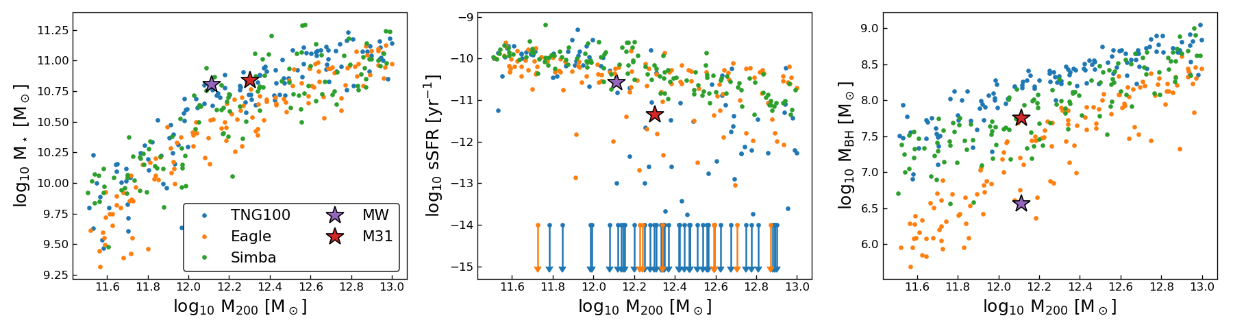
Figure 2: Properties of the galaxies in the three samples (low/medium/high mass) for each of the three simulations (TNG100 in blue, EAGLE in orange, Simba in green). The x-axis of each of the three panels is the halo mass M₂₀₀ in log₁₀. The left panel shows the stellar mass dependence M_⋆, similar to what is shown in 1. We also highlight the location of the Milky Way (purple star), and M31 (red star). The middle panel illustrates the specific star formation rate, sSFR in units of $\mathrm{y}\mathrm{r}^{-1}$, clearly decreasing with increasing halo mass. The right panel shows the SMBH mass dependence, clearly indicating a different trend between the simulations, where EAGLE produces lower mass black holes than TNG100.

2.2.3 Mock X-ray observations

We produce mock observations from the hydro simulations using pyXSIM (see ZuHone & Hallman, 2016), which creates large photon samples from the 3D simulations. We create mock observations from a high spectral resolution imaging instrument assuming a Gaussian PSF with 10 arcsec FWHM using SOXS. We use a detector size of $128\times 128$ pixels with $15\text{\,}\arcsec$ per pixel, yielding a FoV of $$32\text{\,}\mathrm{\SIUnitSymbolArcminute}$\times$32\text{\,}\mathrm{\SIUnitSymbolArcminute}$$. The spectral bandpass covered is 0.2 to 2 keV, with 2 eV FWHM resolution. The X-ray emission is modelled from each emitting, non-star-forming gas cell with $T>$3\text{\times}{10}^{5}\text{\,}\mathrm{K}$$ and $\rho<$5\text{\times}{10}^{-25}\text{\,}\mathrm{c}\mathrm{m}^{-3}$$ (a value of the density close to the star formation density threshold in the TNG simulations). In each galaxy, there is also a small set of isolated gas cells which are abnormally bright in X-rays–these typically have extreme values of cooling time and/or thermal pressure, and on this basis are excluded from the analysis to improve visualizations, but we do not find that leaving them in changes any of our conclusions (see ZuHone et al. submitted, for more details).

The plasma emission of the hot gas surrounding the galaxy is based on the Cloudy emission code (Ferland et al., 2017), and includes the effect of resonant scattering from the CXB, which enhances the O VIIr line (Chakraborty et al., 2020a, 2022). An extensive description is provided in Churazov et al. (2001); Khabibullin & Churazov (2019). In contrast to other emission models, such as APEC/AtomDB (Foster et al., 2012, 2018), we utilize a density-dependent model, that is sensitive to the photo-ionization state of the gas at densities $\lesssim$1\text{\times}{10}^{-4}\text{\,}\mathrm{c}\mathrm{m}^{-3}$$ (see, e.g., Bogdan et al., 2023). We updated the code with respect to Khabibullin & Churazov (2019) to include the latest version of Cloudy, and ensured that the intrinsic resolution matches the sub-eV requirements of a microcalorimeter. The various metal species are independent of each other, allowing a consistent modelling of gas with arbitrary metal abundance patterns.

However, we neglect the effects of resonant scattering from the hot ISM gas in the galaxy (Nelson et al., 2023). We place the low and medium mass samples at a nearby redshift of $z=0.01$, which separates the forbidden O VII line, the C VI line, the O VIII line and the 725 and 739 eV Fe XVII lines from the MW foreground. However, the O VII resonance line is blended with the MW foreground forbidden line. The size of these halos (R₅₀₀) fits well within the assumed field of view of the detector. However, since galaxies in the high mass sample are too large to fit them in the 32x32 arcmin field of view, we chose $z=0.035$ for this sample. This allows us to include the resonance line of O VII, but blends the 739 eV Fe XVII line with MW foreground (see Fig. 3).

The Galactic foreground emission is assumed to consist of a thermal component for the local hot bubble (LHB, temperature $0.1\text{\,}\mathrm{k}\mathrm{e}\mathrm{V}$, McCammon et al., 2002), an absorbed thermal model to account for Galactic halo emission (GHE, temperature of $0.23\text{\,}\mathrm{k}\mathrm{e}\mathrm{V}$, McCammon et al., 2002, and a velocity broadening of $100\text{\,}\mathrm{k}\mathrm{m}\,\mathrm{s}^{-1}$), and the North Polar Spur or hotter halo component (NPS, temperature $0.7\text{\,}\mathrm{k}\mathrm{e}\mathrm{V}$, see Das et al. (2019b); Bluem et al. (2022), also broadened by $100\text{\,}\mathrm{k}\mathrm{m}\,\mathrm{s}^{-1}$). Each thermal component is implemented with the APEC model (Foster et al., 2018) with solar abundances (Anders & Grevesse, 1989), and the absorption with the tbabs model (Wilms et al., 2000) with a hydrogen column density to $1.8\text{\times}{10}^{20}\text{\,}\mathrm{c}\mathrm{m}^{-2}$. The normalizations are $\mathcal{N}_{\rm LHB}=$1.7\text{\times}{10}^{-6}\text{\,}\mathrm{c}\mathrm{m}^{-5}\,\mathrm{a}\mathrm{r}\mathrm{c}\mathrm{m}\mathrm{i}\mathrm{n}^{-2}$$ for the LHB, and $\mathcal{N}_{\rm GHE}=0.43\,\mathcal{N}_{\rm LHB}$ for the GHE, and $\mathcal{N}_{\rm NPS}=0.05\,\mathcal{N}_{\rm LHB}$ for the NPS. The spatial distributions are flat in the mock event files.

The astrophysical background contains unresolved X-ray point sources, mostly distant AGNs (cosmic X-ray background, CXB). On average, the flux distribution of a source follows a powerlaw $S_{\nu}\propto\nu^{-2}$ (De Luca & Molendi, 2004; Hickox & Markevitch, 2006), and the $\log N-\log S$ distribution from Lehmer et al. (2012). The average powerlaw normalization is $4.1\text{\times}{10}^{-7}\text{\,}\mathrm{p}\mathrm{h}\mathrm{t}\,\mathrm{s}^{-1}\,\mathrm{k}\mathrm{e}\mathrm{V}^{-1}\,\mathrm{c}\mathrm{m}^{-2}$ after excising the brightest 50 point sources from the event file, which make up half of the total CXB flux (and about 3% of the FoV area).

Considerations on the particle background based on Athena X-IFU (Barret et al., 2013, 2018) studies showed that a spectral component due to Galactic cosmic rays will be a factor of 30 to 60 lower than the second lowest component, the CXB. We included a conservative estimate on the residual particle background, after anti-coincidence filtering, of $1\text{\,}\mathrm{c}\mathrm{t}\mathrm{s}\,\mathrm{s}^{-1}\,\mathrm{k}\mathrm{e}\mathrm{V}^{-1}$ for the field of view. The particle background is assumed to have a flat spectrum and no spatial features. Our mock event files include all the above-mentioned components and simulate a 1 Ms observation.

2.3 Analysis

The analysis of the mock event files relies partly on existing software, such as CIAO, but most routines are re-implemented in python using astropy (The Astropy Collaboration et al., 2013, 2018), and the scipy packages.

2.3.1 Preparation

Our simulated mock event files use coordinates that reflect the physical pixels of the LEM detector array with $15\text{\,}\mathrm{a}\mathrm{r}\mathrm{c}\mathrm{s}\mathrm{e}\mathrm{c}$ width and height. However, the optics and mirror assembly of LEM reach a spatial resolution of $10\text{\,}\mathrm{a}\mathrm{r}\mathrm{c}\mathrm{s}\mathrm{e}\mathrm{c}$, which will be utilized through Lissajous-dithering. Therefore, we oversample the detector pixels by a factor of 2 for all images that are produced, also internally, e.g. for point source detection. To start the analysis of the simulated event files, we visually inspect the images and spectra around the O VII(f) emission line. The exact spectral location of the peak of the line emission is specified, in order to center the extraction region for line surface brightness profiles later on. Then we define the emission weighted center using the emission around the O VII(f) line ($\pm$2\text{\,}\mathrm{e}\mathrm{V}$$), which is typically within a few pixels of the center of the FoV.

2.3.2 Point sources

Following these initial tasks, we use the wavdetect algorithm included in the CIAO 4.14 package (Fruscione et al., 2006) to detect point sources from the CXB in the observation, and in the corresponding background file. Since the point sources are expected to have a continuum powerlaw spectrum, we use a broad band image, $250950\text{\,}\mathrm{e}\mathrm{V}$ for the detection. While several hundred point sources are typically detected, we select the 50 most significant and brightest sources, which contribute about 50% to the total CXB flux, but only about 2-3 % of the detector area. The least significant of the top 50 sources is still detected at $100\sigma$. An example of the detected sources can be seen in the top left panel of Fig. 4. The area of these 50 point sources is masked out in the observation and background event file for the following analysis steps. More details on the point source contribution is given in section A.

2.3.3 Surface brightness profiles

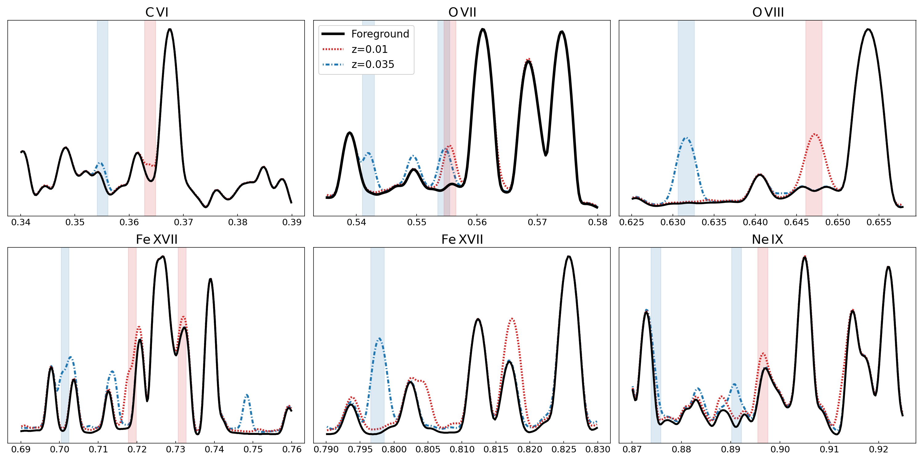
Figure 3: Spectral windows that are used for the surface brightness extraction. The x-axes of the panels are in keV, and the y-axis is flux in arbitrary units. The black lines show a spectral model of the total background, i.e. Milky Way foreground, and CXB emission. We show the CGM emission with a thermal model at $0.2\text{\,}\mathrm{k}\mathrm{e}\mathrm{V}$, marked by the blue and red lines for $z=0.035$ and $z=0.01$, respectively. The small windows marked by the colored bars are used to distinguish the CGM from the foreground emission. Note that the 826 eV line of Fe XVII is only used for the high mass/high redshift galaxies.

For our radial surface brightness profiles we extract the counts in the mock event files with respect to the center of the galaxy halo. We define the center as the emission-weighted peak in the O VII(f) image. Counts are extracted in a narrow 2 eV spectral window centered at the redshifted line energies ($367.49\text{\,}\mathrm{e}\mathrm{V}$ for C VI, $560.97\text{\,}\mathrm{e}\mathrm{V}$ for O VII(f), $574.04\text{\,}\mathrm{e}\mathrm{V}$ for O VII(r), $653.72\text{\,}\mathrm{e}\mathrm{V}$ for O VIII, and $$725.09\text{\,}\mathrm{e}\mathrm{V}$,$727.00\text{\,}\mathrm{e}\mathrm{V}$,$739.02\text{\,}\mathrm{e}\mathrm{V}$,$825.75\text{\,}\mathrm{e}\mathrm{V}$$ for Fe XVII. The 2 eV spectral window is the optimal width in terms of signal-to-noise, and it includes 76% of the line counts. The area of the 50 brightest point sources is masked.

Figure 3 shows the redshifted spectral extraction with respect to the foreground emission for several interesting line windows considered here. The red shaded regions correspond to the extraction for the nearby ($z=0.01$) galaxies, the blue shaded regions to the more distant ($z=0.035$) galaxies. For the case of O VII, we can use the forbidden and resonant lines at $z=0.035$, while for the nearby galaxies at $z=0.01$, we only use the forbidden line. In the case of Fe XVII, we can use three lines, the 725 eV, 727eV and the 739 eV lines at lower redshift, while at $z=0.035$, we extract the 725 eV, 727 eV and the 826 eV lines.

We note that we compute the radial bin size adaptively, where we require the bins to have a minimum signal-to-noise ratio of 3, and also require the source-to-background ratio in each bin to be at least 10%, to not be dominated by statistical or systematic uncertainties. We estimate the background counts based on a simulated blank field observation with only foreground and CXB background components, where we repeat the same steps that were performed for the CGM observation, namely the point source detection, as this field has a different realization of the CXB point sources (see details in section A.2). The background counts are estimated from the whole field of view (minus the excised point sources) to reduce the uncertainty in the background. Since this background estimate assumes a field of view averaged residual CXB contribution (point sources that are fainter than the 50 brightest that are excluded), we introduce a scaling factor to the background counts in each annulus, based on the broad band emission ($\pm$200\text{\,}\mathrm{e}\mathrm{V}$$ around the line) of the continuum CXB sources (see appendix A.2).

The individual profiles are then interpolated if needed, and a median profile (of all the galaxies in the sample) is created at fixed fractions of R₅₀₀. The scatter (68.3%) at each radii between the ensembles of profiles represents the galaxy-to-galaxy scatter.

2.3.4 Structural clumping in the gas

While the radial surface brightness profiles demonstrate LEM’s ability to detect the CGM to large distances, it does not quantify the level of substructure present in the gas at a given radius, and how well LEM can detect this. It is expected that different feedback mechanisms leave imprints in the CGM. Stellar feedback is able to push out gas from the inner region near the disk to larger radii and cause an anisotropic distribution, especially within intermediate radii ($\sim 0.5R_{500}$). A very dominant AGN will have a major impact on the gas distribution in the halo. After several feedback cycles, it is expected that the gas distribution gets smoothed by the impact of the AGN.

To capture this information in our mock observations, we derive the ratio of the average squared density to the square of the average density (e.g., Nagai & Lau, 2011), which characterizes the azimuthal asymmetry and clumpiness in the X-ray gas. We trace this quantity observationally by calculating the median emission line surface brightness profile over small sectors $S(r)_{\rm median}$, and compare it to the average surface brightness $S(r)_{\rm mean}$:

$$\mathcal{C}(r)=\frac{\langle\rho^{2}\rangle}{\langle\rho\rangle^{2}}\approx\frac{S_{\rm mean}(r)}{S_{\rm median}(r)}~{}.$$ (1)

$\mathcal{C}(r)$, where $\rho$ is the gas density, also referred to in the literature as the emissivity bias (Eckert et al., 2015). Typical values from observations range from 1, meaning no azimuthal asymmetry or substructure, to about 2 at large radii. Emission from a single line is more prone to vary, due to temperature variations in the gas. We calculate $\mathcal{C}$ in annuli of width $0.25R_{500}$ from stacked images of the O VII(f), the O VIII, C VI, and the Fe XVII 725 eV line. Therefore, we combine the signal from the three emission lines, which also increases the signal to noise. We trace the substructure out to a radius of $R_{500}$ (4 radial bins), while using 8 sectors (45 deg each). We then stack the $\mathcal{C}$ profiles for galaxies to derive the median profile. We notice that especially for lower mass halos, the scatter in $\mathcal{C}$ is substantial. Since we are only interested in the type of galaxy where $\mathcal{C}$ is significantly larger than 1, we use the range of $\mathcal{C}$ values in the 50^th to 75^th percentile as a diagnostic.

2.3.5 Spectral analysis

We can use the signal of the various emissions lines to constrain the CGM temperature. The model fitting of small spectral windows around the emission lines allows us to extract even more information from the CGM observations, such as the relative line-of-sight velocity, and the abundance ratio, which gives further insights on gas motion, outflows, enrichment history, and re-heating processes. We utilize this technique to make spectral maps.

For the spectral mapping, we extract 8 eV windows of the spectrum from circular regions based on the brightness distribution of the three lines, O VII(f), O VIII, and Fe XVII, through an adaptive binning technique (see O’Sullivan et al., 2013; Kim et al., 2019), which we briefly describe here: At every pixel of the combined line image, we derive a radius at which we reach a threshold signal to noise. This radius can be different for neighboring pixels. The spectral extraction region for each pixel is given by the determined radius. As a consequence, the spectra of neighboring pixels are not independent, and we will oversample the map. We use a signal-to-noise of 10 as a threshold parameter (which is sufficient given the emission line takes only a small portion of the 8 eV wide spectral window), and we do not include pixels if the radius has to be larger than $7\text{\,}\mathrm{\SIUnitSymbolArcminute}$.

We assume the foreground model and CXB models are not known apriori, and constrain their parameters through spectral fitting of a separate background spectrum. This background spectrum is extracted from the same observation, using a region outside the central $15\text{\,}\mathrm{\SIUnitSymbolArcminute}$ radius, and masking extended bright regions within $R_{500}$. We apply the mask that has been determined for removing the point sources in the background observation. This leaves about 30% of the detector area for the background spectrum, which is enough to measure all parameters (temperatures and normalizations) with high precision. The spectral extraction is done using the CIAO tools dmextract, and dmgroup to have a grouped spectrum file with at least one count per bin.

For the spectral fitting, we use Sherpa (Freeman et al., 2001; Burke et al., 2020), which is distributed with CIAO, and also provides the Xspec models, such as APEC and tbabs (Arnaud, 1996; Foster et al., 2012). We model the background emission with two absorbed APEC models (including thermal and velocity broadening with a velocity of $100\text{\,}\mathrm{k}\mathrm{m}\,\mathrm{s}^{-1}$, and one unabsorbed APEC model plus one absorbed power low to fit the background components in the mock observations (see section 2.2). We also add CGM components, but we are mostly interested in constraining the background and foreground model parameters with this outer region where the background dominates. We are able to reproduce the input background parameters within 2% relative accuracy. We save the best-fit values of the temperatures and normalizations for the next steps.

We then determine the extraction region for spectra through adaptive binning. During the spectral fitting, we use the previously determined background parameters and freeze these values (the normalizations are scaled by the ratio of region size to the background region). These foreground parameters are well determined from a large extraction area (statistical uncertainties on a percent level). We only leave the CXB powerlaw normalization free to vary, since each spectral region can contain a slightly different population of CXB sources, while the CXB normalization from the background spectrum is just the average over a larger area. We also include a Gaussian smoothing (gsmooth, with $\alpha=1$) of the CGM components to account for any broadening of the lines. Our CGM emission model consists of 19 absorbed components: The individual elements C, N, O, Ne, Mg, Si, S, Fe, plus a model for all other elements, one component for each element that includes the effect of resonant scatter of the cosmic microwave background (Ferland et al., 2017; Khabibullin & Churazov, 2019), and one component for the emission in plasma without metals. The normalization of the resonant scattered components is frozen to half the normalization of the corresponding element, since we removed about half the flux from CXB emission through the point source masking. Each of the CGM components has a temperature, redshift, and intrinsic hydrogen column density (for the photo-ionization), and all parameters are linked, so there is effectively only a single temperature plasma component.

We use Cash statistics (Cash, 1979) for the fitting of the input spectrum and select several spectral windows:

• Carbon: The lowest energy window from $33.4\text{\,}\mathrm{\SIUnitSymbolAngstrom}$ to $34.1\text{\,}\mathrm{\SIUnitSymbolAngstrom}$ ($363.5\text{\,}\mathrm{e}\mathrm{V}$ to $371.5\text{\,}\mathrm{e}\mathrm{V}$) contains the C VI line which peaks at $1.28\text{\times}{10}^{6}\text{\,}\mathrm{K}$ ($0.11\text{\,}\mathrm{k}\mathrm{e}\mathrm{V}$) temperature, but also significant emission from N and other metals.

• Nitrogen: Emission around the N VII line (peak temperature of $1.97\text{\times}{10}^{6}\text{\,}\mathrm{K}$, or $0.17\text{\,}\mathrm{k}\mathrm{e}\mathrm{V}$), with the window ranging from $24.6\text{\,}\mathrm{\SIUnitSymbolAngstrom}$ to $25\text{\,}\mathrm{\SIUnitSymbolAngstrom}$ ($496\text{\,}\mathrm{e}\mathrm{V}$ to $505\text{\,}\mathrm{e}\mathrm{V}$), also contains emission from C and other metals.

• Oxygen (2 windows): The O VII triplet (from $21.4\text{\,}\mathrm{\SIUnitSymbolAngstrom}$ to $22.3\text{\,}\mathrm{\SIUnitSymbolAngstrom}$ ($557\text{\,}\mathrm{e}\mathrm{V}$ to $579\text{\,}\mathrm{e}\mathrm{V}$), and O VIII $18.8\text{\,}\mathrm{\SIUnitSymbolAngstrom}$ to $19.1\text{\,}\mathrm{\SIUnitSymbolAngstrom}$ ($650\text{\,}\mathrm{e}\mathrm{V}$ to $658\text{\,}\mathrm{e}\mathrm{V}$) lines peak at $1.97\text{\times}{10}^{6}\text{\,}\mathrm{K}$ ($0.17\text{\,}\mathrm{k}\mathrm{e}\mathrm{V}$) and $3.13\text{\times}{10}^{6}\text{\,}\mathrm{K}$ ($0.27\text{\,}\mathrm{k}\mathrm{e}\mathrm{V}$), respectively. Of the O VII triplets, the forbidden line is very interesting, since it is not blended with the foreground lines in our low redshift samples. O VIII is dominant at higher temperatures and can help to constrain the temperatures in the regions.

• Iron: The Fe XVII complex window from $16.7\text{\,}\mathrm{\SIUnitSymbolAngstrom}$ to $17.2\text{\,}\mathrm{\SIUnitSymbolAngstrom}$ ($721\text{\,}\mathrm{e}\mathrm{V}$ to $743\text{\,}\mathrm{e}\mathrm{V}$) is very bright, peaks at a temperature of $5\text{\times}{10}^{6}\text{\,}\mathrm{K}$ ($0.43\text{\,}\mathrm{k}\mathrm{e}\mathrm{V}$), and contains several weaker transitions of other elements, such as O VII.

• Neon: The Ne IX triplet window from $13.4\text{\,}\mathrm{\SIUnitSymbolAngstrom}$ to $13.8\text{\,}\mathrm{\SIUnitSymbolAngstrom}$ ($901\text{\,}\mathrm{e}\mathrm{V}$ to $926\text{\,}\mathrm{e}\mathrm{V}$) is not very bright and only visible in some galaxies. The peak temperature is $3.95\text{\times}{10}^{6}\text{\,}\mathrm{K}$ ($0.34\text{\,}\mathrm{k}\mathrm{e}\mathrm{V}$).

Note that all the windows are redshifted according to the true (simulated) redshift of the galaxy. Unconstrained parameters are frozen to a default value. The reduced $\chi^{2}$ are typically very close to 1. After the best-fit parameters are found, we use the MCMC sampling method integrated into Sherpa to find the parameter uncertainties using the Metropolis Hastings algorithm.

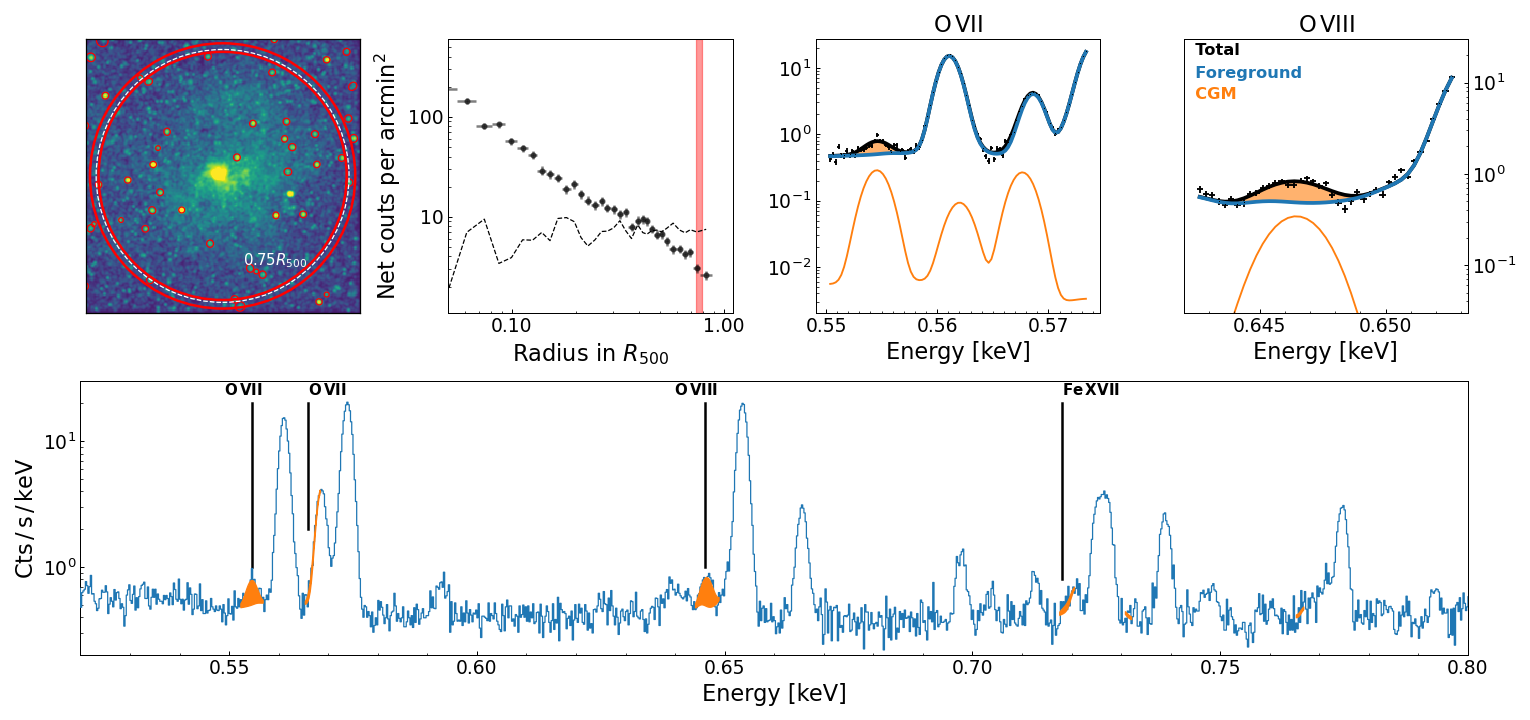
Figure 4: Example for a $10^{11.18}\,$\mathrm{M}_{\odot}$$ stellar mass galaxy with $R_{500}=$243\text{\,}\mathrm{k}\mathrm{p}\mathrm{c}$$ (TNG50, ID 358608, at $z=0.01$). A map of the narrow band O VIII emission (including background/foreground) is shown in the top left panel, where all the detected point sources are marked by small red circles, and the extraction region used for the other panels is shown as a large red annulus around the $0.75\,$\mathrm{R}_{500}$$ marker. A surface brightness profile of the O VIII line is shown in second to right top panel, and the spectral region of both, the O VII and  VIII emission including the Milky Way foreground, in the two top left panels. A wider spectrum is shown in the bottom panel, with the CGM emission in excess of the foreground/background emission as the orange shaded area.

3 Results

The results of our analysis laid out in the following sections demonstrate the extraordinary capabilities of LEM for detecting and characterizing the CGM emission. As an example, we show in Figure 4 the line emission image, surface brightness profile and spectral extraction regions for a TNG100 galaxy at the upper mass end ($\log_{10}M_{\star}/M_{\odot}=11.18$, and $R_{500}=$243\text{\,}\mathrm{k}\mathrm{p}\mathrm{c}$$) placed at $z=0.01$. The top left panel shows the stacked O VII, O VIII, and Fe XVII image which fills the LEM field of view. The top right panel shows the surface brightness profile, and the background level (dashed line). At the red extraction region around $0.75R_{500}$ and $1\text{\,}\mathrm{\SIUnitSymbolArcminute}$ width, the CGM emission still reaches 50% of the background. The bottom panel of Fig. 4 shows the overall spectrum from 544 to $800\text{\,}\mathrm{e}\mathrm{V}$ with the prominent CGM emission lines indicated. The two middle panels show closeups of the O VII and O VIII windows with the foreground model overplotted in blue, and the CGM model in orange.

In the following, we systematically analyze the two samples for each of the three simulations.

3.1 Line surface brightness profiles

We extract surface brightness profiles of 4 important emission line windows, C VI, O VII(f), O VIII, and Fe XVII, which peak at different plasma temperatures ($0.11\text{\,}\mathrm{k}\mathrm{e}\mathrm{V}$, $0.17\text{\,}\mathrm{k}\mathrm{e}\mathrm{V}$, $0.27\text{\,}\mathrm{k}\mathrm{e}\mathrm{V}$, and $0.43\text{\,}\mathrm{k}\mathrm{e}\mathrm{V}$, respectively). The profiles are extracted in a $2\text{\,}\mathrm{e}\mathrm{V}$ window around the redshifted line energy, which minimizes the contamination with foreground lines from the MW. We extract a profile of a simulated background/foreground observation in the same fashion and subtract this from the observation of the CGM.

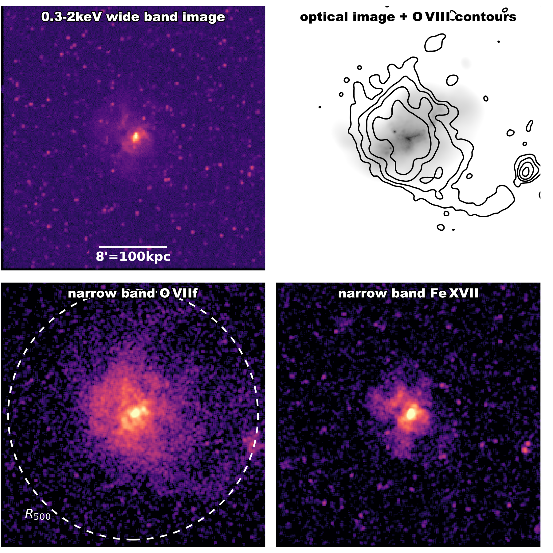
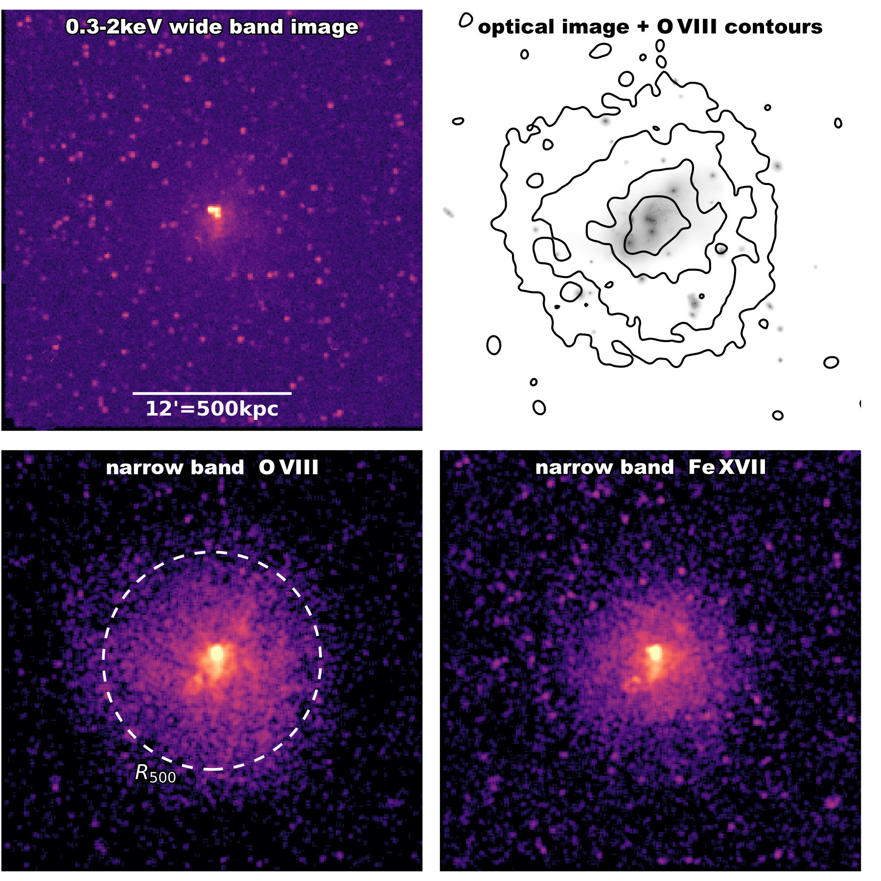
Figure 5: Illustrating the capabilities of a LEM-like mission for mapping the CGM: Left: Galaxy halo of the size of the Milky Way at z=0.01 (TNG100, ID 417281). Right: High mass galaxy at z=0.035 (TNG100, ID 292921). The 4 panels in each image show the broad band image similar to a CCD resolution instrument (top left), the optical r-band image with O VIII contours (top right), the O VII(f) or O VIII image with R₅₀₀ indicated (bottom left), and the Fe XVII image (bottom right).

Figure 3 shows the spectra of a single temperature plasma at $z=0.01$ (blue) and $z=0.035$ (red). The spectra contain the foreground emission, which we show also without the redshifted CGM (only foreground) as black lines. It is clear that already at redshift $z=0.01$, the CGM line emission is well separated from the foreground lines.

Each of the low, medium, and high mass samples contain 40 galaxies, while the former two have the galaxies at $z=0.01$, and the latter at $z=0.035$. More details on the individual galaxies, such as stellar mas, gas mass, and black hole mass, are given in Tables 1, 2, 3, and 4.

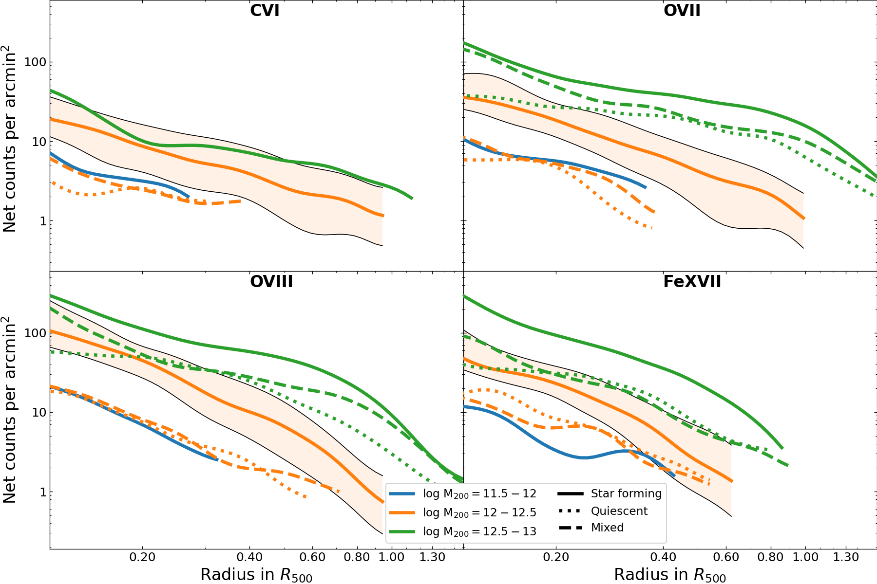
Figure 6: Median profiles of the CGM emission from the EAGLE galaxies, binned by halo mass ($M_{200}$). The solid, dotted, and dashed lines correspond to star-forming, quiescent, and mixed subsamples, respectively. Blue, orange, and green curves show the low, medium, and high mass galaxy halos, respectively. The orange shaded region represents the 68% scatter, shown only for star-forming medium mass galaxies for visibility purposes.

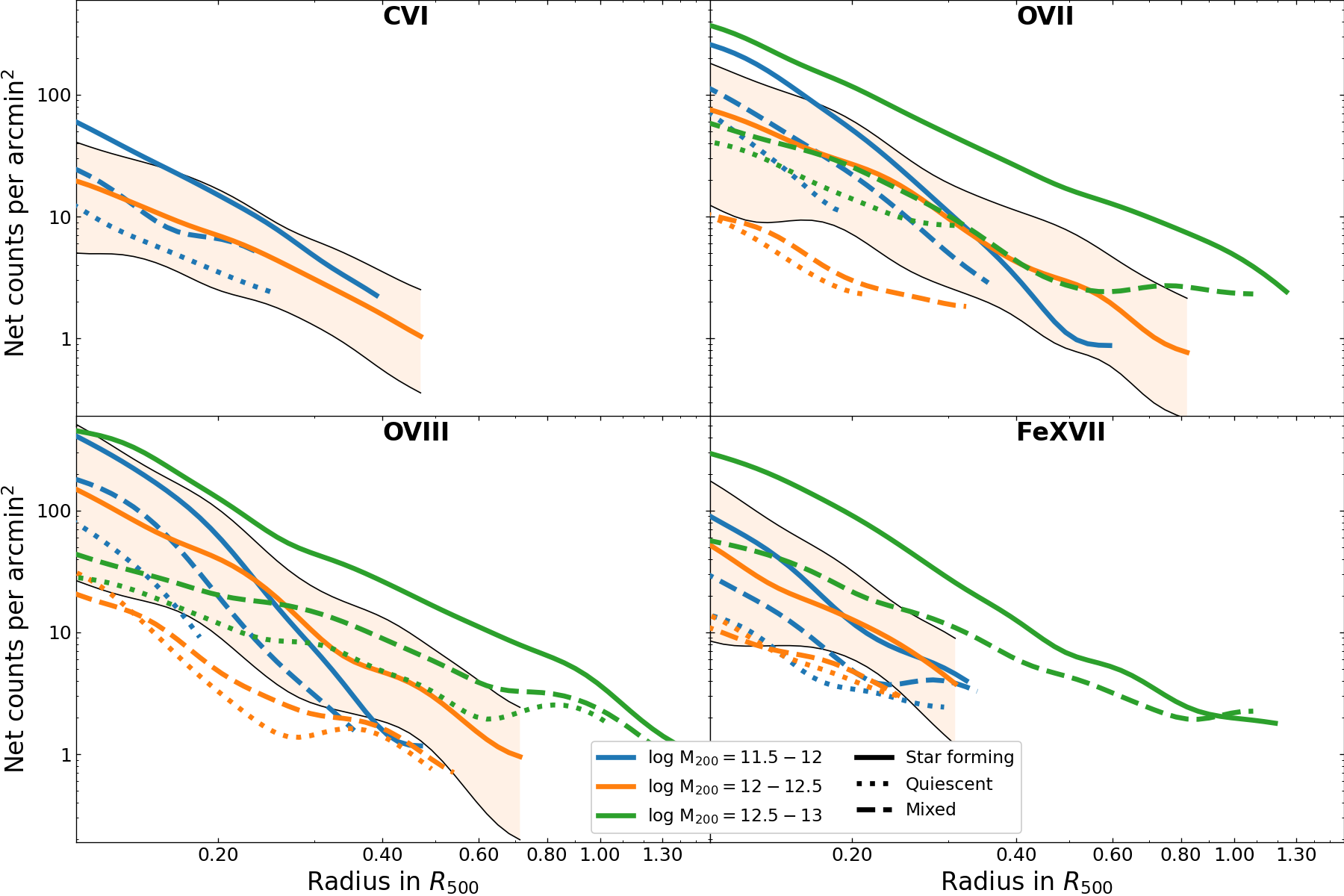
Figure 7: As Fig. 6, but for TNG100 galaxy halos.

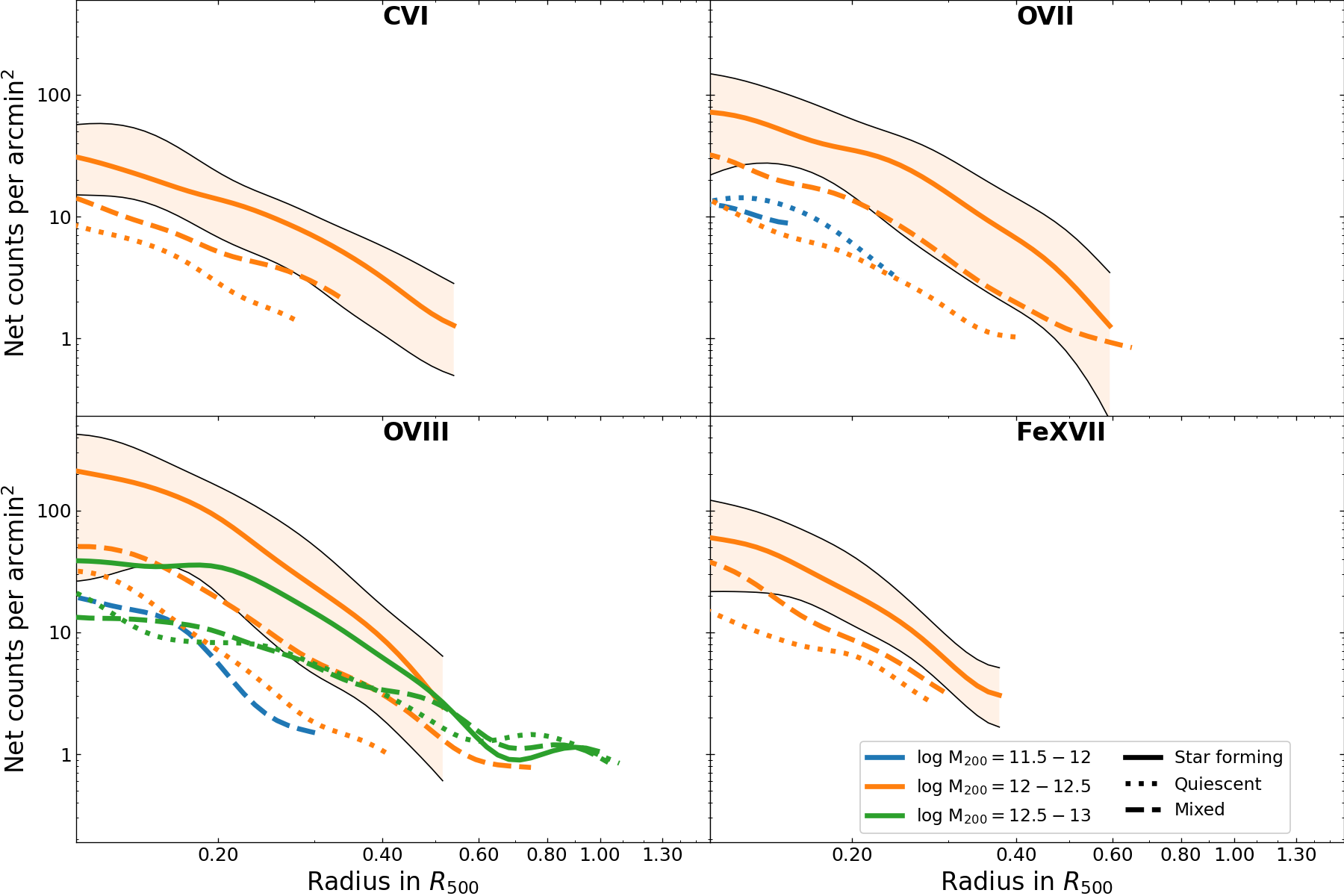
Figure 8: As Fig. 6 but for Simba galaxy halos.

We analyze the median profile with the radius scaled by R₅₀₀. Each of the three mass-defined samples is subdivided into thirds based on the star formation rate. We conservatively consider CGM detection if the measured signal is at least 10% of the background, and the signal-to-noise of each extracted radial bin is at least 3. We show these profiles in Figs. 6, 7, and 8 for EAGLE, TNG100, and Simba, respectively. The low-mass, medium-mass, and high-mass samples are shown in blue, orange, and green, respectively. The subsamples are shown in solid, dotted, and dashed lines for the top, lowest, and intermediate thirds, respectively. Therefore, each line is the median profile of 13 or 14 galaxies. We note that the star formation subsample is defined by percentiles of the galaxies in the sample, and therefore does not necessarily reflect globally star-forming or quiescent galaxies. The typical 68% scatter is shown for the star-forming, medium mass sample as the orange region.

We detect the C VI, O VII, O VIII, and Fe XVII lines in emission in all simulations. Based on the galaxy mass, all simulations detect the CGM emission out to R₅₀₀. Simba is clearly the faintest. However, there is significant scatter between the galaxies of a single simulation, and between the different simulations. O VIII can be detected out R₂₀₀ ($1.5R_{500}$) for the more massive galaxies in TNG100 and EAGLE. The O VIII line is the brightest, with the highest number of counts and a relatively low background, followed by O VII and Fe XVII. While C VI can be detected in most galaxies, it is very weak in Simba. For the oxygen and carbon, TNG100 and EAGLE are comparable, but TNG100 typically has a steeper shape, leading to a smaller detection radius. Especially for galaxies in the low and medium mass sample (blue, orange), TNG100 has a clear trend that galaxies with higher star formation are also brighter (solid line above dashed line, and the dotted line is lowest). This has also been pointed out, e.g., by Oppenheimer et al. (2020). The lowest mass galaxies with little star formation appear very faint in EAGLE. However, for the medium mass sample, we only partially find the same trend with star formation rate (solid line highest, but dotted and dashed lines comparable). For the high mass sample, we find in both, TNG100 and EAGLE, that at larger radii close to $R_{500}$ the brightness is independent of star formation (see also Oppenheimer et al., 2020).

The medium mass sample shows oxygen and iron emission at about 0.6 to $1\,R_{500}$ in both simulations, EAGLE and TNG. For C VI we find a big difference between EAGLE and TNG100, where in EAGLE carbon is detected out to $0.8\,R_{500}$, and in TNG100 only to about $0.3\,R_{500}$. The visibility of the high mass galaxies placed at $z=0.035$ is not limited by the field of view, and can therefore can be traced far beyond R₅₀₀ as in the case of O VII (both resonant and forbidden line combined, see Fig. 3) and O VIII. We also can detect Fe XVII in both, EAGLE and TNG100, nearly to R₅₀₀, depending on the star formation rate. C VI was not detected in the high mass TNG100 galaxies, but it is very clearly visible in EAGLE.

Clearly, Fe XVII is detected best in EAGLE, likely because some of the galaxy halos are hotter. The difference in the visibility of C VI between EAGLE and TNG100 at higher halo masses is not explained by the higher EAGLE CGM temperatures, but possibly by a different metal composition, as carbon is produced also by AGB stars. Comparing the scatter between the galaxy halos of a given sample, we notice a slightly larger scatter among TNG100 galaxies. The scatter of the CGM profiles between the Simba galaxies can only be measured at smaller radii.

3.2 Emission line ratios

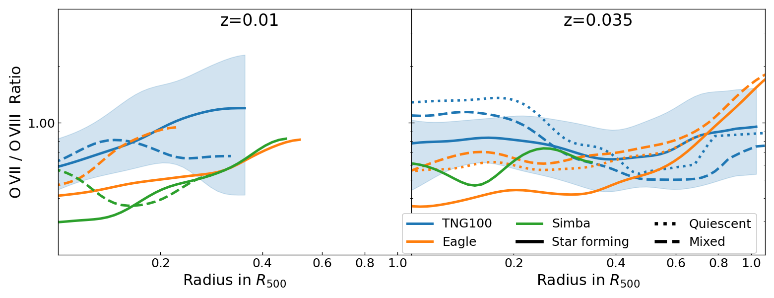
Figure 9: The O VII to O VIII line ratios for the low and medium mass samples (left), and high mass samples at larger redshift (right). As in the profile plots, the solid, dotted, and dashed lines correspond to star-forming, quiescent, and mixed subsamples, respectively, while the orange curves show EAGLE galaxies, the blue curves TNG100, and the green curves Simba. The blue shaded region represents the 68% scatter, shown only for star-forming TNG100 galaxies for visibility purposes.

If the hot gas in and around galaxies is not isothermal, we expect the shape of emission line profiles that are sensitive to different gas temperatures, to reflect this. In the case of the same element (e.g., oxygen) the line ratio, e.g., O VII and O VIII, is proportional to the gas temperature. At large radii with low gas densities, photo-ionization becomes important and changes the line ratios. When comparing the emission lines of different elements (e.g., C VI and Fe XVII), the conclusions are less clear, since not only the temperature changes in the gas, but the enrichment mechanism: SNIa contribute significantly to the abundance of iron, but not to that of carbon or oxygen. We note that we only include galaxy halos simulated with TNG100 and EAGLE here.

Figure 9 shows the O VII to O VIII line ratio for the same samples that were shown in section 3.1. Looking at the nearby galaxies in Fig. 9 (left), we notice a systematic offset between star-forming TNG100 and EAGLE galaxies, where the EAGLE ratios are always below the TNG100 ones. This indicates that the EAGLE galaxy halos are systematically hotter within the covered radius $<0.5R_{500}$ (see also Truong et al. submitted). For the mixed star forming/quiescent galaxies (the quiescent ones alone did not provide enough statistics), we find comparable line ratios within the scatter of the samples (compare e.g., Truong et al. submitted). Unfortunately, statistics only allow us to derive line ratios to about $0.4\,R_{500}$, until which we see a rising line ratio, indicating a hotter core and cooler outer regions (Fig. 9). For the high mass galaxy halos (Fig. 9, right), we see a similar trend of star-forming galaxies being hotter in TNG100 (lower O VII to O VIII ratio). TNG100 halos appear almost isothermal (constant line ratio), while EAGLE galaxies have an increasing line ratio toward the outer regions, and become even steeper beyond $0.6\,R_{500}$. At these large radii, the difference between star-forming and quiescent galaxies appears to vanish: The impact of star formation is most prominent in the core. In principle, we need to include the effects of photo-ionization in our interpretation of line ratios at large radii, since at very low plasma densities the assumption of collisional ionization equilibrium (CIE) is no longer applicable. However, simulating several line ratios with fixed plasma temperature and only changing the density showed that above a density of $3\text{\times}{10}^{-5}\text{\,}\mathrm{c}\mathrm{m}^{-2}$ the changes in the ratio are less than 5-6%. Densities within $R_{500}$ are expected to be larger than that (e.g., Bogdán et al., 2013b). We note that in dense regions with column densities above ${10}^{21}\text{\,}\mathrm{c}\mathrm{m}^{-2}$, the O VII to O VIII ratio will be affected by electron scattering escape (Chakraborty et al., 2020b).

3.3 Substructure in the CGM emission

In order to analyze the substructure that can be detected in the mock observations, we apply the method introduced in section 2.3.4. The clumping factor, $\mathcal{C}$, is calculated for the TNG100 and EAGLE halos in all three mass samples.

As pointed out before, a clumping factor of 1 means that there was no clumping detected, and observations have shown that it can raise typically up to 2 at $R_{500}$. This can be associated with the substructure in the outskirts being accreted. For clusters Eckert et al. (2013, 2015); Zhuravleva et al. (2015) have observed very low clumping factor values, even at $R_{500}$, while Simionescu et al. (2011) found higher values for the Perseus cluster.

Since the calculation of the clumping factor of a single emission line, like the O VII, could bias the results due to the sensitivity to temperature changes in the CGM, we use the stacked signal of the O VII, O VIII, and Fe XVII lines. The combined samples cover a wide range of galaxy halos in terms of mass, star formation rate, or temperature. Therefore, we divided the sample into galaxies with a central SMBH below the median SMBH mass, and the ones above, shown in Fig. 10 as dark shaded and light shaded regions.

We find an interesting trend for the black hole mass distinction: We do not see any difference in EAGLE for different SMBH masses (all values outside the core are within 1 to 1.1, see Fig. 10 right). However, galaxies in TNG100 show a dichotomy (Fig. 10 left), as we find systematically higher $\mathcal{C}$ for lower SMBH masses outside $0.4R_{500}$, while massive SMBHs show a very similar trend between EAGLE and TNG100. Simba galaxy halos are generally fainter and statistical uncertainties are larger, but lower mass SMBH appear similar to the trend in TNG100, as they have higher $\mathcal{C}$, but less significant. This trend found for the TNG100 galaxy halos is consistent with simulations by Rasia et al. (2014); Planelles et al. (2014, 2017), in which they argue that SNe and especially AGN feedback can smooth out the gas distribution. While TNG100 and Simba have efficient AGN feedback that can push out the gas and increase the kinematics, EAGLE can pressurize the gas more efficiently. It should be noted that the numerical schemes, hydrodynamic solvers, and sub-grid physics, especially of feedback in the simulations suites are different, which will impact the gas distributions. A Smoothed Particle Hydrodynamics (SPH) simulation will also produce a smoothed gas distribution (e.g., Rasia et al., 2014).

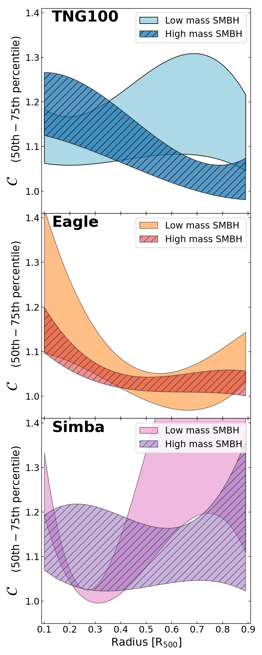
Figure 10: Azimuthal asymmetry as a function of radius, parameterized by the clumping factor $\mathcal{C}$ (defined in section 2.3.4). We show the 50^th to 75^th percentile of the sample to illustrate the galaxy halos among the sample with high substructure, which are different in TNG100 (left) and EAGLE (right). The darker, shaded area is for higher mass black holes in the galaxy sample, while the lighter shaded area shows low mass black holes.

3.4 Spectral analysis

The detectability of CGM emission lines with LEM out to large radii offers the opportunity to not only derive one-dimensional profiles, but, to map the emission out to R₅₀₀, and measure temperatures, line-of-sight velocities, and abundance ratios. We described our spectral fitting approach in section 2.3.5, and apply it here to two galaxies selected from TNG50 of the IllustrisTNG project (Nelson et al., 2019a; Pillepich et al., 2019). With the smaller box size, the TNG50 simulation has higher resolution with respect to TNG100 (used for the profiles). Since we do not want to select a large number of galaxies, but rather study two examples in more detail, a larger simulation box won’t provide any advantage.

We explore two galaxy halos in more detail: The first galaxy (358608) has a halo mass of $10^{12.7}\,$\mathrm{M}_{\odot}$$, which would place it in our high mass sample. It has a relatively high stellar mass of $10^{11.18}\,$\mathrm{M}_{\odot}$$, and a high star formation rate, $3.87\text{\,}\mathrm{M}_{\odot}\,\mathrm{y}\mathrm{r}^{-1}$. With a mass of $10^{8.64}\,$\mathrm{M}_{\odot}$$ its central SMBH is relatively dominant, and we expect both AGN and stellar feedback to be present here. $R_{500}=$242\text{\,}\mathrm{k}\mathrm{p}\mathrm{c}$$ exceeds slightly the LEM FoV at $z=0.01$, which yields $19.7\text{\,}\mathrm{\SIUnitSymbolArcminute}$. Figure 11 a) shows the observed (i.e., including background and foreground treatment) O VIII emission: We see a bright core and extended CGM emission out to the edge of the field of view ($16\text{\,}\mathrm{\SIUnitSymbolArcminute}$ radius or $195\text{\,}\mathrm{k}\mathrm{p}\mathrm{c}$). Brighter filaments extend to the north (forming a rim around a lower surface brightness region), and south-east, perpendicular to the galactic disk, which is edge-on and oriented south-west to north-east (see the optical r-band image tracing the stellar population in Fig. 11 b ). The optical image also shows a smaller structure, about 100 kpc to the west, which is a smaller galaxy. It also has an X-ray counterpart in the O VIII image. The X-ray brightness in the simulation (Fig. 11 c) shows the “true” distribution of the hot gas, which is very filamentary. The temperature map of this system (Fig. 11 d) is derived from the relative line strengths of the O VII(f), O VIII, and Fe XVII lines, and will be most sensitive to trace temperature between 0.15 and 0.45 keV. The typical statistical uncertainties vary between $0.03\text{\,}\mathrm{k}\mathrm{e}\mathrm{V}$ and $0.005\text{\,}\mathrm{k}\mathrm{e}\mathrm{V}$, so relative uncertainties range between 1% and 10% (see Fig. 11 d). Comparing this observed temperature map with the idealized, emission weighted temperature (0.5-1 keV band) derived from the simulation (Fig 11 f), we can reproduce the brighter parts to the north of the core and the south-east. The emission weighted temperature is even higher in these regions, mostly because the lines that we used from our mock observation to probe the gas temperature are not sensitive enough to the hotter gas components. We note that a mass weighted temperature will be biased toward high mass, low temperature gas cells, and therefore be lower than the emission weighted temperature, which more closely reflects our measured quantity in the mock observations.

The velocity map (Fig. 11 g ) reveals a split between east and west, with an average difference between the two sides of about $300\text{\,}\mathrm{k}\mathrm{m}\,\mathrm{s}^{-1}$. As this is most pronounced in the central region, it can be explained by the rotation of the disk. The higher velocity gas (red region southeast of the core) is likely an outflow, since it overlaps with the hotter regions. The predicted, emission weighted velocity map from the simulation (Fig. 11 i) confirms this, as it shows structures that are very consistent: The central rotation of the disk, the higher velocity part to the south-east, and the large scale velocity structure of the hot gas. A subsequent paper (ZuHone et al. submitted) will analyze the velocity structure of simulated galaxy halos in great detail. The statistical uncertainty mainly depends on the number of counts in a line. With our adaptive binning described in section 2.3.5, we get a velocity uncertainty of about 25 to $45\text{\,}\mathrm{k}\mathrm{m}\,\mathrm{s}^{-1}$ in the brighter central regions, and about $80\text{\,}\mathrm{k}\mathrm{m}\,\mathrm{s}^{-1}$ in the lower surface brightness region north-east of the center. We assumed conservatively a 2 eV response across the field of view.

We also show the observed oxygen-to-iron ratio (Fig. 11 j). This abundance ratio is sensitive to the enrichment history, mainly the supernovae SNIa versus core-collapsed supernovae (Mernier et al., 2020). We find typical values in the central region $[\rm O/Fe]=-0.3$ ($Z_{\rm O}/Z_{\rm Fe}=0.5$), and values closer to $[\rm O/Fe]=0$ ($Z_{\rm O}/Z_{\rm Fe}=1$) and above, in the outer regions. This is consistent with the predicted O/Fe brightness from the simulation (Fig. 11 l), which shows the center and outflows to be more Fe-rich. For galaxy clusters and groups, the oxygen abundance has been found to be flat, while iron is centrally peaked Werner et al., 2006; Mernier et al., 2017; Vogelsberger et al., 2018, which leads to an increasing O/Fe profile. A similar trend can be expected for galaxies (Geisler et al., 2007; Segers et al., 2016; Matthee & Schaye, 2018). Some regions, especially in the south-east, have very high oxygen abundances, up to 2.5. Typical uncertainties range from 10-20% in the center to 70% in the faintest regions.

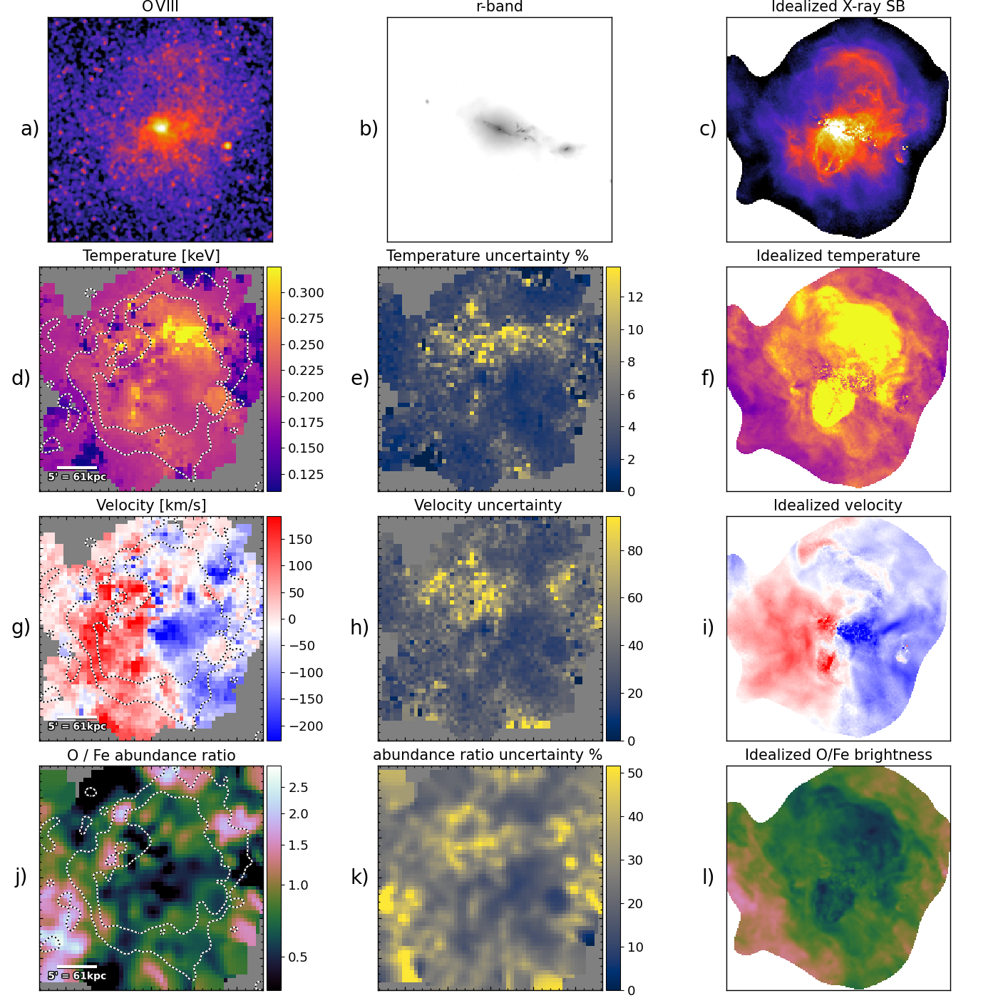
Figure 11: Spectral map of galaxy 358608 from TNG50 (for details see text), showing observed O VIII surface brightness (a), and the predicted optical r-band signal (b), the simulated X-ray brightness (c), the observed temperature in keV (c, and error map d) from a simultaneous fit to O VII, O VIII, and Fe XVII lines), the emission weighted temperature from the simulation (f), the observed average line velocity shift in $\mathrm{k}\mathrm{m}\,\mathrm{s}^{-1}$ (g, and error map h), the predicted, emission weighted LOS velocity in the simulation (i), the observed O/Fe abundance ratio (g, and error map h), and the predicted O/Fe brightness ratio in the simulation (l).

The second galaxy (467415) that we map in detail is also selected from TNG50, but with a lower halo mass of $10^{12.32}\,$\mathrm{M}_{\odot}$$, which would place it in the medium mass sample. The stellar mass, $10^{10.94}\,$\mathrm{M}_{\odot}$$ is relatively high for its size, and the star formation of $8.9\text{\,}\mathrm{M}_{\odot}\,\mathrm{y}\mathrm{r}^{1-}$ might still dominate its halo environment. Also, its SMBH mass is at the higher end with $10^{8.33}\,$\mathrm{M}_{\odot}$$, which makes this another interesting target to study the effects of stellar and AGN feedback. The radius, $R_{500}=$183\text{\,}\mathrm{k}\mathrm{p}\mathrm{c}$$, is within the LEM field of view at $z=0.01$. The observed O VIII emission (Fig. 12 a) is brightest in the center, but extends out to almost 100 kpc, and some filaments beyond that. The distribution is not azimuthally uniform, but seems to be aligned along filaments, mainly to the south-east, the north, and a narrow region to the west. The r-band contours in Fig. 12 b show one single galaxy at the center, and some much smaller and fainter structures to the south, possibly small satellite galaxies. Figure 12 c displays the X-ray surface brightness in the simulation.

The observed temperature map (Fig. 12 d, and the error map e) shows the hottest emission ($\sim$0.3\text{\,}\mathrm{k}\mathrm{e}\mathrm{V}$$) near the center of the galaxy, while the temperature in the outer filaments drops to $0.18\text{\,}\mathrm{k}\mathrm{e}\mathrm{V}$. We identify slightly hotter structures, extending from the south-east to the north-west, while the north-east to south-west axis has cooler gas. The uncertainties are again in the 1% to 10% range. The temperatures are broadly consistent with emission weighted temperature in the simulation (Fig 12 f).

The velocity (Fig. 12 g, and the error map h) ranges from $250\text{\,}\mathrm{k}\mathrm{m}\,\mathrm{s}^{-1}$ in the south-east to $-250\text{\,}\mathrm{k}\mathrm{m}\,\mathrm{s}^{-1}$ in the north-west, outside the stellar disk. These are even higher velocities than the within first, more massive galaxy. This coincides with the hotter regions in the temperature map, and is consistent with the predicted velocity from the simulation (Fig. 12 i). Along the faint, low-temperature regions in the south-west and north-east, the velocities are lower than the surrounding. Statistical uncertainties are similar to the other galaxy, ranging from 20 to $80\text{\,}\mathrm{k}\mathrm{m}\,\mathrm{s}^{-1}$.

Lastly, the oxygen-iron map (Fig. 12 j, and the error map k) has typical values between 0.5 and 1, but also several small regions exceed 1 by far (statistical uncertainties are between 20% and 70%). It is consistent with the predicted O/Fe brightness in the simulation (Fig. 12 l), where the iron rich gas is again in the center and along the high velocity, high temperature trajectory from the south-east to slightly north of the core.

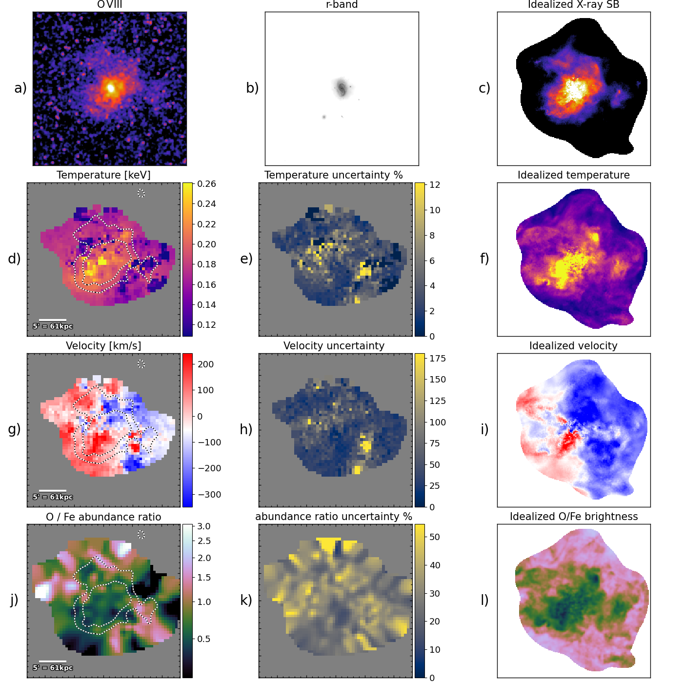
Figure 12: As for Fig. 11, but for the lower mass galaxy from TNG50 (ID 467415, details in the text).

The level of detail that is revealed in these spectral maps is unprecedented for galaxy-sized halos. Typical spectral maps from CCD based detectors (e.g., Chandra or XMM-Newton) can only reach large radii (e.g., R₅₀₀) for galaxy clusters and massive galaxy groups, however, without any line-of-sight velocity information.

4 Discussion

4.1 Tracing the CGM with X-ray microcalorimeters

The extended gaseous halos around MW-like galaxies are predicted by simulations, and have been detected in stacked broad-band images. Constraining their extent, brightness profile, azimuthal distribution, and enrichment with various elements for individual galaxies will allow us to distinguish between simulation models and ultimately understand the changing feedback processes of galaxies on various scales. The X-ray continuum emission of these galaxies is very faint, but the bright emission lines, namely O VII, O VIII, and Fe XVII, are clearly detectable over the local background and foreground. Selecting a narrow $\sim$2\text{\,}\mathrm{e}\mathrm{V}$$ energy band around these lines results in a high signal to noise detection with LEM, in a 1 Ms exposure of a $z=0.01$ galaxy, and even allows the mapping of these galaxy halos. Only focusing on emission lines and not having the continuum information will still allow the majority of science questions to be answered: How is the hot gas distributed, and what are the relative metal abundances (e.g., wrt iron). Only the degeneracy between metallicity and density cannot be broken.

The faint CGM line emission around individual, nearby spiral and elliptical galaxies cannot be detected and mapped with current X-ray CCD instruments due to the bright Milky-Way foreground emission. Even state-of-the-art DEPFET detectors such as the Athena/WFI (Meidinger et al., 2017) with its $\sim$80\text{\,}\mathrm{e}\mathrm{V}$$ energy resolution will not be able to distinguish the CGM emission lines from the much brighter foreground. A galaxy redshift of at least $0.12$ is necessary to shift the O VIII line from the foreground, which will also reduce the apparent size of the galaxy to about $1\text{\,}\mathrm{a}\mathrm{r}\mathrm{c}\mathrm{m}\mathrm{i}\mathrm{n}$, and the total flux to about 8% with respect to a galaxy at redshift $0.01$.

The development of microcalorimeters marks the start of a new epoch in X-ray astronomy, reaching unprecedented energy resolution, while spatially resolving the structure of the source. The currently planned Athena/X-IFU instrument (Barret et al., 2018) will have a large effective area and good spatial resolution. However the field-of-view of $\sim 5\times 5$\mathrm{a}\mathrm{r}\mathrm{c}\mathrm{m}\mathrm{i}\mathrm{n}^{2}$$ (before reformulation) is clearly not sufficient to observe the extended CGM of nearby galaxies. At $z=0.01$ a Milky-Way-sized galaxy has $R_{500}\approx 15\arcmin$, and therefore requires about 30 pointings. Moving to a higher redshift and utilizing Athena’s large effective area can reduce the required amount of observing time to a factor of 5-10 times what a LEM-like mission would need. Galaxies at $z\gg 0.01$ will also not offer the same amount of structure that can be resolved. Since simulations predict variance between galaxies, also based e.g., on the star formation rate, one would like to cover a medium-sized sample of 10 to 20 galaxies.

The X-Ray Imaging and Spectroscopy Mission (XRISM, Tashiro et al., 2018 expected to be launched in 2023) will also have a microcalorimeter onboard. However, its field-of-view is limited to only $$3\text{\,}\mathrm{\SIUnitSymbolArcminute}$\times$3\text{\,}\mathrm{\SIUnitSymbolArcminute}$$, the effective area is about 10-15 times smaller than LEM, and together with the arcmin spatial resolution and only $6\times 6$ pixels, it will not be able to map the extended CGM.

Other mission concepts with a large effective area microcalorimeter include the Line Emission Mapper (Kraft et al., 2022), and HUBS (Zhang et al., 2022). While HUBS does not have enough spatial resolution to map the structure, and distinguish X-ray point sources in the field, LEM is clearly optimized to the CGM science by having sufficient energy resolution ($2\text{\,}\mathrm{e}\mathrm{V}$), a large effective area similar to XMM-Newton, a $10\text{\,}\mathrm{a}\mathrm{r}\mathrm{c}\mathrm{s}\mathrm{e}\mathrm{c}$ PSF, and a large field-of-view of $\sim$900\text{\,}\mathrm{a}\mathrm{r}\mathrm{c}\mathrm{m}\mathrm{i}\mathrm{n}^{2}$$, allowing one to map nearby galaxies in a single pointing. In contrast to typical X-ray observations of faint, diffuse sources, the instrumental background level plays only a minor role when using a narrow energy band of a microcalorimeter: The requirement for Athena/X-IFU is to reach an internal particle background level of $5\text{\times}{10}^{-3}\text{\,}\mathrm{c}\mathrm{t}\mathrm{s}\,\mathrm{s}^{-1}\,\mathrm{c}\mathrm{m}^{-2}\,\mathrm{k}\mathrm{e}\mathrm{V}^{-1}$ (Lotti et al., 2021). This should be achieved through a graded anti-coincidence shield, while the background is predicted to be about an order of magnitude higher without the shielding. For our results, we assumed a constant particle background level in the soft band of $8.6\text{\times}{10}^{-2}\text{\,}\mathrm{c}\mathrm{t}\mathrm{s}\,\mathrm{s}^{-1}\,\mathrm{c}\mathrm{m}^{-2}\,\mathrm{k}\mathrm{e}\mathrm{v}^{-1}$, which is more than 15 times higher the Athena requirement. The foreground emission however, scales with the effective area of the mirror. In the case of LEM, it will be the dominant background component, and even at the foreground continuum around the O VIII line, the particle background is still below all other components (foreground and CXB).

4.2 Model distinction

We have demonstrated that a LEM-like microcalorimeter will be able to detect the CGM of MW-mass galaxies to large radii $\sim R_{500}$, even in low mass galaxies below the “transition” regime (Fig. 1). Long exposure times with CCD instruments such as Chandra ACIS or XMM-Newton EPIC spent on individual massive galaxies have revealed only the innermost part of the CGM, and at best give us a vague idea of the temperature structure, especially if they are not in an ongoing starburst phase. Bogdán et al. (2013a) used Chandra to image NGC 266, a massive (M${}_{200}\approx$8\text{\times}{10}^{12}\text{\,}\mathrm{M}_{\odot}$$), nearby galaxy, and detected the CGM out to about 60 kpc, which is about 20% of R₅₀₀. Bogdán et al. (2017) used XMM-Newton to detect and characterize the CGM around the massive galaxy NGC 6753, which has a virial mass of ${10}^{13}\text{\,}\mathrm{M}_{\odot}$. The authors could reliably make a detection out to 50 kpc, before background systematics made any conclusions impossible. This is about 17% of R₅₀₀. These exceptional cases demonstrate, that only with massive efforts, we are currently able to explore up to 1% of the volume that the CGM fills out to R₅₀₀, and this only for the most massive, hand-picked galaxies, which are at the high mass end. Our mock observations show that with a large grasp microcalorimeter we can not only detect these type of galaxies out to R₂₀₀ in individual lines, such as O VIII, but also map their dynamical, thermal, and chemical abundance. These galaxies are expected to be dominated by AGN feedback, which we see as outbursts in the velocity map or the O/Fe ratio map. Features in the abundance ratio map, such as high O/Fe ratios maybe indicative of strong early feedback or a recent starburst, whereas a high abundance of metals from AGB winds, such as carbon and nitrogen may be evidence for efficient gas entrainment from the ISM in SNe-driven winds (e.g., Nomoto et al., 2006; Das et al., 2019b; Carr et al., 2023).

A LEM-like instrument will explore unknown territory by also mapping galaxies of much lower mass, down to M${}_{200}\approx$3\text{\times}{10}^{11}\text{\,}\mathrm{M}_{\odot}$$, which has not been done so far. In this regime, we do not expect AGNs to be important in the feedback cycle, while stellar winds are expected to enrich and reheat the CGM.

The details of the transition from stellar to AGN feedback are largely not understood and are implemented ad-hoc in simulations to match some observational constraints, such as stellar scaling relations ($M-\sigma$, $M_{\star}-M_{\rm halo}$, galaxy morphologies, quiescent fractions as a function of stellar mass, and SFR$-z$ relations). Many measurements can be conducted that will lead to a new understanding of the processes within the CGM: Central regions, where a spectral continuum of the CGM emission can be measured, allowing us to constrain the absolute metal abundance, and at larger radii, the steepening of the X-ray line emission to distinguish the contribution from SN feedback, as seen, e.g., between EAGLE and TNG100, where TNG100 produces centrally peaked profiles with a steeper decrease in surface brightness. Measurements of the X-ray luminosities, surface brightness profiles, temperature distributions that relate to the outflow energies, will allow one to distinguish if feedback is instantaneously stopping a cooling flow, if the cumulative effect from preventing gas phases to cool, or if the gas is ejected from the the disk (Davies et al., 2019b; Truong et al., 2020; Terrazas et al., 2020; Oppenheimer et al., 2020). With a few assumptions such as a metallicity profile, a total gas mass can be derived. Supplementary observations such as Sunyaev-Zeldovich (SZ, e.g., Wu et al., 2020; Bregman et al., 2022; Moser et al., 2022), or fast radio bursts (FRB, e.g., Ravi, 2019; Macquart et al., 2020; Wu & McQuinn, 2023) will also help to derive the gas mass. The impact of the central AGN will be observed in the range of azimuthal asymmetry observed in the CGM emission.

Chadayammuri et al. (2022) and Comparat et al. (2022) have demonstrated through stacking of optically detected galaxies in the eROSITA Final Equatorial Depth Survey (eFEDS) that the X-ray bright CGM exists even in low mass galaxies. Based on these results, simulations such as EAGLE and TNG100 are likely underestimating the surface brightness, especially in the low mass regime (see, e.g., the $2.5\text{\times}{10}^{10}\text{\,}\mathrm{M}_{\odot}$ stellar mass bin in Fig. 4 of Chadayammuri et al., 2022, which is a factor of 3-5 above the simulation predictions). Furthermore, the dichotomy between star forming galaxies being brighter in simulations with respect to quiescent galaxies, might not be true, at least not to the extent that it is predicted. Quiescent galaxies with little to no star formation tend to have massive and dominant AGNs, and are well-suited to understand the AGN cycles. These results cast doubt on the validity of the Simba CGM profiles, as Simba appears to drive gas to too large radii, making the galaxy halos fainter than observed by Chadayammuri et al. (2022). However, stacking cannot replace systematic analyses of individual galaxies as it might be biased by a few bright objects. Simba also appears to be too X-ray faint, compared to low-mass groups (Robson & Davé, 2020), as the energy output from the bipolar jets evacuates the halos.

4.3 Observing strategies

In the previous sections we demonstrated that a LEM-like mission with a large grasp microcalorimeter will be able to map nearby galaxies over a wide range of mass, star formation rate, and black hole mass. We argued that an instrument such as the Athena X-IFU will not be able to dedicate enough observing time to this science area. However, even an observatory such as LEM will not be able to spend 1 Ms on 120 galaxies that we assumed to have observations available (40 in each of the three mass samples).

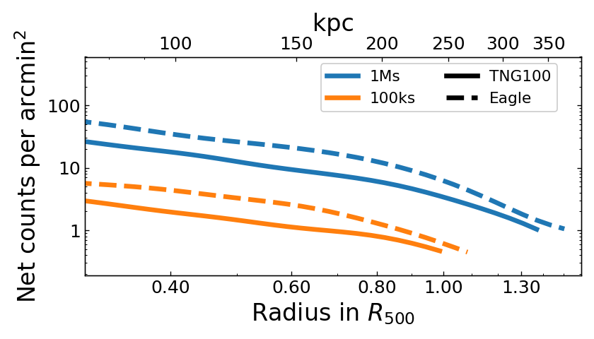
Figure 13: LEM median O VIII surface brightness profile of the total high mass sample of EAGLE (dashed lines) and TNG100 (solid lines) for two simulated exposure times, 1 Ms (blue), and 100 ks (orange).

We test the impact on constraining the line surface brightness distribution with shorter observations (Fig. 13), and found that even with 100 ks per galaxy, a LEM-like mission will be able to map the O VIII emission out to R₅₀₀, in both EAGLE and TNG100 simulated galaxies. In an observing plan for a LEM-like mission, fainter galaxies will take up significantly more observing time, especially in the crucial transition regime of Milky Way mass galaxies. Having 10 low, 10 medium, and 10 high mass galaxies, where each galaxy is observed by 1 Ms with the exception of the high mass halos (100 ks), one can achieve such an ambitious program within about 20 Ms, which is a typical directed science program for a probe class mission. While the trend of the average properties (e.g., O VIII brightness) in each mass bin is important, the dispersion around the median, also will be important to understand. Therefore, galaxies should be selected to cover a range of properties that might shape the CGM, such as the stellar mass $M_{\star}$ at a given halo mass, the star formation rate, and the mass of the supermassive black hole.

We also tested whether dedicated background observations are necessary, or whether surface brightness profiles can be extracted using a model of the foreground and background emission. This model can be fit to the same observation in an outer region, and then constrain the expected background plus foreground counts in each annulus at the CGM line spectral window. This method achieves comparable results, and reduces the overhead, but requires a good model of the foreground spectrum.

5 Summary

Mapping the X-ray emission of the hot circumgalactic medium (CGM) is the key to understanding the evolution of galaxies from smaller galaxies with star formation driven feedback, to larger, quiescent galaxies. Milky Way mass galaxies appear to be at the transition point between these regimes. However, the current generation of X-ray instruments are unable to capture the emission from the hot CGM, that is dominant in the soft X-ray band, and distinguish it from the bright Milky Way foreground. We demonstrate that a high spectral resolution microcalorimeter with a large field of view and large effective area cannot only detect the CGM line emission to R₅₀₀, but also can map the individual physical properties such as temperature and velocity. A mission designed to study the hot CGM, similar to the Line Emission Mapper probe concept, will transform all fields of astrophysics (Kraft et al., 2022).

We created realistic mock observations, based on hydrodynamical simulations from EAGLE, IllustrisTNG, and Simba, for a large effective area instrument with 2 eV spectral resolution, and a $$32\text{\,}\mathrm{\SIUnitSymbolArcminute}$\times$32\text{\,}\mathrm{\SIUnitSymbolArcminute}$$ FoV. We included all background and foreground components in these mock observations. The galaxies span a mass range from $\log M_{200}[M_{\odot}]=11.5-13$, and have been divided into three samples, based on their halo mass to represent the dominating feedback regime. For the mock observations, the low and medium mass galaxies (up to $\log M_{200}[M_{\odot}]\leq 12.5$) are placed at $z=0.01$, while the high mass galaxies are at $z=0.035$, and an exposure time of $1\text{\,}\mathrm{M}\mathrm{s}$ is used. For each galaxy we constrain the surface brightness profile of the O VII(f), O VIII, Fe XVII (725 and 729 eV), and C VI. For galaxies at $z=0.035$ we also include the O VII(r) and the Fe XVII (826 eV) lines, but have to omit the Fe XVII (729 eV) line, since it is blended with the Milky Way foreground. Our findings are summarized as follows:

• The median galaxy surface brightness profile for Milky Way sized galaxies at $z=0.01$ can be traced to R₅₀₀, which is typically $170\text{\,}\mathrm{k}\mathrm{p}\mathrm{c}$ or $14\text{\,}\mathrm{\SIUnitSymbolArcminute}$.

• The CGM in more massive galaxy halos up to $\log M_{200}=13$ at $z=0.035$ can be measured out to R₂₀₀. Even for the lowest mass halos (down to $\log M_{200}=11.5$ we typically will measure CGM emission out to $\sim 0.5R_{500}$.

• The O VIII emission line is brightest in most cases, followed by O VII and Fe XVII.

• Subdividing the galaxy samples by star formation rate reveals that star forming TNG100 galaxies are brighter in the core.

• There is significant scatter in the CGM brightness due to galaxy-to-galaxy variation. Also the different simulations produce slightly different CGM luminosities at a given mass scale, where EAGLE galaxies are brightest, especially at higher masses, and Simba galaxies are typically the faintest, due to the strong AGN feedback expelling the gas.

We demonstrate that the O VII to O VIII line ratio in the mock observations can be used as a temperature tracer out to R₅₀₀ for more massive galaxies at $z=0.035$, and to $0.5R_{500}$ for the less massive galaxies at $z=0.01$. We find that EAGLE galaxies are hotter in the center compared to TNG100, while having similar line ratios to TNG100 at large radii.

We are able to map the substructure of galaxies out to R₅₀₀ through by quantifying the azimuthal asymmetry. Interestingly, we find that TNG100 and Simba galaxies with a smaller SMBH reach high values of substructure beyond $0.4R_{500}$, while EAGLE galaxies do not show that level of clumping. For massive SMBHs, all simulations predict lower CGM clumping factors. This observable appears to be crucial to understand the mechanisms of AGN feedback, as it directly points to the efficiency of the AGN to pressurize the CGM gas.

Finally, we test the 2D properties of the gaseous halos around galaxies with spectral maps of properties, such as the temperature, the line-of-sight velocity, and the O/Fe ratio. Together, these quantities can be used to pin-point signatures of AGN feedback, such as the AGN duty cycle, or energy output.

Appendix A Analysis details

The analysis of simulated microcalorimeter observations of nearby galaxies resembles the traditional X-ray analysis. However, a few details have been altered to take advantage of the high spectral resolution. We describe this here in more detail.

A.1 Point source removal

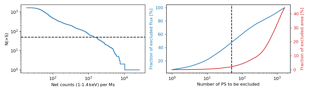
Figure 14: Removal of point sources in the observation. Left: Cumulative number counts as a function of flux (in net counts). Right: The blue line represents the fraction of excised flux in point sources as a function of the number of point sources (highest flux sources first), and the red line shows, for the same number of excised point sources, the area fraction that is masked.

The point sources in the simulated event files are detected through wavdetect in the $11.4\text{\,}\mathrm{k}\mathrm{e}\mathrm{V}$ band, where only CXB and NXB dominate. At softer energies the Galactic emission will dominate, and at higher energies the particle background will dilute the CXB signal due to the decrease in effective area. We show in Fig. 14 (left) the distribution of cumulative number counts as a function of the threshold flux $S$ (in net source counts within a 1 Ms observation). The distribution is consistent with the expected trend based on the Chandra observations by Lehmer et al. (2012), where a broken powerlaw is found for distant AGNs and galaxies. If we excise the 50 brightest sources (Fig. 14 right) we remove about 50% of the total flux in point sources, while only removing about 2% of the detector area. For the 100 brightest sources we would remove more than 4% of the area and 60% of the flux, and if we removed 250 sources, we would excise 75% of the flux and almost 10% of the total detector area.

A.2 Surface brightness extraction

In order to trace the emission lines (such as O VIII) in a narrow band out to large radii, it is important to quantify the background precisely. While the MW foreground should be greatly reduced, due to the redshift, the exact level of the background is still crucial, when we want to make a detection with a signal that is only 10% of the total background level. We separate the background components into MW foreground (Local Hot Bubble - LHB, Galactic Halo Emission - GHE, and North Polar Spur - NPS), the unresolved/un-removed point source contribution from distant AGNs and galaxies (Cosmic X-ray Background - CXB), and the interaction of charged particles (galactic cosmic rays) with the detector and/or the satellite (producing secondary particles, such as fluorescent X-rays or electrons), which is not focused by the mirrors (Non X-ray Background - NXB). The modeling of these components in our simulated X-ray observations has been described in section 2.2.

To estimate the background counts in a narrow band at the redshifted CGM line, we take a blank field observation without a science target, and spatially close to the observation of each nearby galaxy of interest. We assume that the MW foreground emission does not vary within the FoV of our observation, and is also consistent with the MW foreground in the blank field observation. The same assumption is made for the NXB, although its contribution is less important at the emission lines of interest. Our focus is set on the CXB contribution to the total background, as it is different not only between the blank field and the galaxy observation, but also varies slightly from each extraction region (annulus) of the surface brightness profile. Therefore, we include a CXB correction factor to the blank field background counts, that is determined from the hard band (e.g., $11.4\text{\,}\mathrm{k}\mathrm{e}\mathrm{V}$), where the MW component is insignificant.

We label the extracted total counts (CGM and total background) in a narrow line band and small extraction region within our observation as ${\rm cts}^{\rm Obs}_{\rm line}$. We define the counts in the broad band and the blank field observation (Bkg) accordingly,

$${\rm cts}^{\rm Obs}_{\rm line} = {\rm CGM}^{\rm Obs}_{\rm line}+{\rm MW}^{\rm Obs}_{\rm line}+{\rm CXB}^{\rm Obs}_{\rm line}+{\rm NXB}^{\rm Obs}_{\rm line}={\rm CGM}^{\rm Obs}_{\rm line}+\mathcal{B}^{\rm Obs}_{\rm line}$$ (A1)

$${\rm cts}^{\rm Obs}_{\rm broad} = {\rm CGM}^{\rm Obs}_{\rm broad}+{\rm MW}^{\rm Obs}_{\rm broad}+{\rm CXB}^{\rm Obs}_{\rm broad}+{\rm NXB}^{\rm Obs}_{\rm broad}={\rm CGM}^{\rm Obs}_{\rm broad}+\mathcal{B}^{\rm Obs}_{\rm broad}$$ (A2)

$${\rm cts}^{\rm Bkg}_{\rm line} = {\rm MW}^{\rm Bkg}_{\rm line}+{\rm CXB}^{\rm Bkg}_{\rm line}+{\rm NXB}^{\rm Bkg}_{\rm line}=\mathcal{B}^{\rm Bkg}_{\rm line}$$ (A3)

$${\rm cts}^{\rm Bkg}_{\rm broad} = {\rm MW}^{\rm Bkg}_{\rm broad}+{\rm CXB}^{\rm Bkg}_{\rm broad}+{\rm NXB}^{\rm Bkg}_{\rm broad}=\mathcal{B}^{\rm Bkg}_{\rm broad}~{}.$$ (A4)

Note that the MW and NXB components scale between the observation and blank field region only with the area (the observing time has already been taken into account), and in the broad band, the CGM component has no real contribution. We utilize a broad band above 1 keV (e.g., $11.4\text{\,}\mathrm{k}\mathrm{e}\mathrm{V}$, see Fig. 15), to estimate the difference in the CXB between our extraction region in the observation and the total blank field (whole FoV).

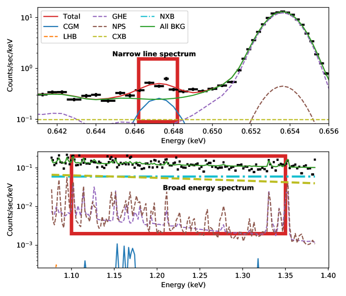
Figure 15: Narrow and broad bands to estimate the CXB scaling of the total background.

We derive a scaling factor,

$$f_{\rm broad}=\frac{{\rm cts}^{\rm Obs}_{\rm broad}}{f_{A}\times\mathcal{B}^{\rm Bkg}_{\rm broad}}~{},$$ (A5)

where $f_{A}$ is the ratio of the extraction area of the observation and the background. $f_{\rm broad}$ is typically close to one, especially if the extraction region in the observation is large (outer annuli). In order to minimize Poisson noise, we estimate the narrow line band background from the entire blank field observation and scale it by the area and $f_{\rm broad}$. We tested this method with a randomly chosen galaxy halo from TNG100 (ID 419061), and define 7 radial bins of $0.15R_{500}$ width to reach an outer radius of $1.05R_{500}$. In each of these regions, we extracted the spectrum from the observation, and fitted it with the model components (see, e.g., Fig. 15), so we have a precise knowledge of background components and the CGM emission. From the fitted model components, we are able to calculate the precise total background in each annulus $\mathcal{B^{\rm Obs}_{\rm line}}$, as well as the CGM counts ${\rm CGM}^{\rm Obs}_{\rm line}$, and make a comparison with the corrected blank field background estimate, $\mathcal{B}^{\rm Bkg}_{\rm line}\times f_{\rm broad}$. We find that the difference in counts between the actual background ,$\mathcal{B^{\rm Obs}_{\rm line}}$ , and the blank field predicted background is always much less than 1% of the CGM counts in each annulus (reaching 0.5% around R₅₀₀). Therefore, we employ this method of scaling the blank field by the broad band CXB contribution to estimate the background. Deriving the background from the spectral fit is computationally expensive and not feasible for each galaxy and extraction region.

In order to define statistically significant radial bins of the surface brightness profile, we require a minimum signal to noise ratio of 3. The signal is directly calculated from the measured ${\rm cts}^{\rm Obs}_{\rm line}$ minus the background estimate $\mathcal{B}^{\rm Bkg}_{\rm line}\times f_{\rm broad}$. The noise is assumed to be

$${\rm Noise}=\sqrt{{\rm cts}^{\rm Obs}_{\rm line}+\mathcal{B}^{\rm Obs}_{\rm line}\times(1-f_{\rm broad})+0.1\times\mathcal{B}^{\rm Obs}_{\rm line}}~{},$$ (A6)

where we account for systematic uncertainties in the background, as well as uncertainties in the CXB contribution.

We also tested the impact of MW foreground uncertainties on the narrow line counts. With the typical uncertainties of the foreground model fitting (using only the narrow lines of C VI, O VII, O VIII, and Fe XVII) in the temperature, e.g., of the LHB, we find a difference in background counts of less than 1% of the CGM counts.

Appendix B List of simulated galaxy halos

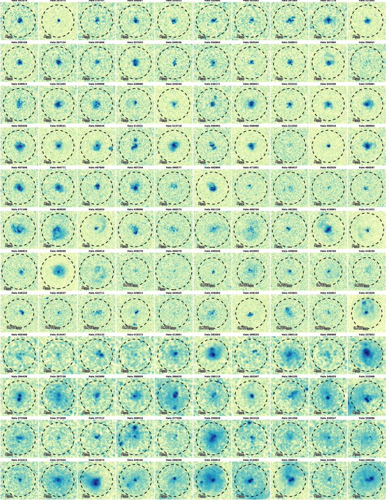
Figure 16: Stacked O VII(f) and O VIII images of the TNG100 galaxy halos.

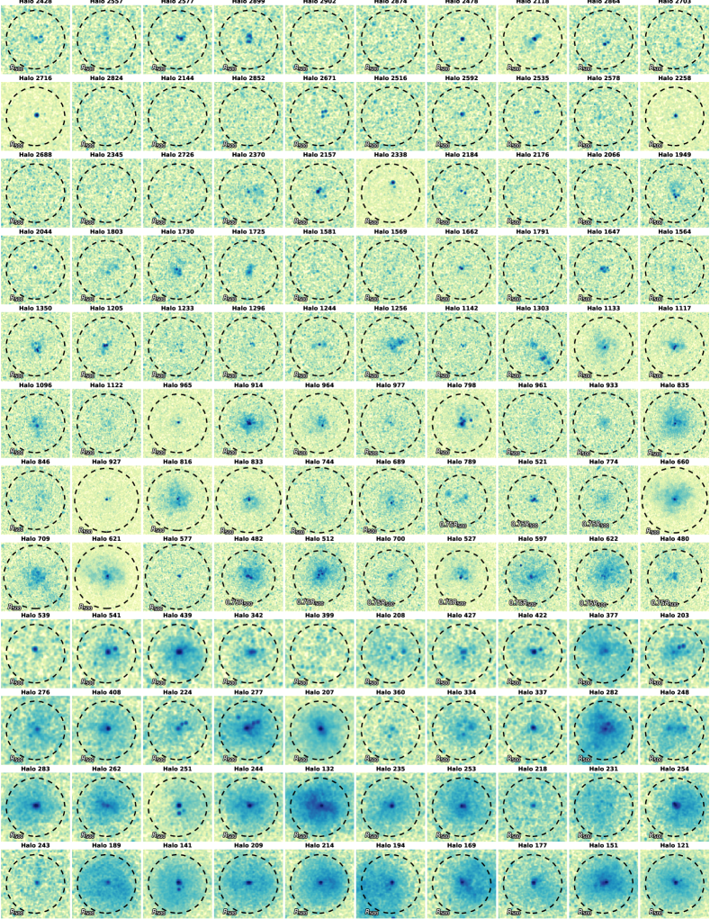
Figure 17: Stacked O VII(f) and O VIII images of the EAGLE galaxy halos.

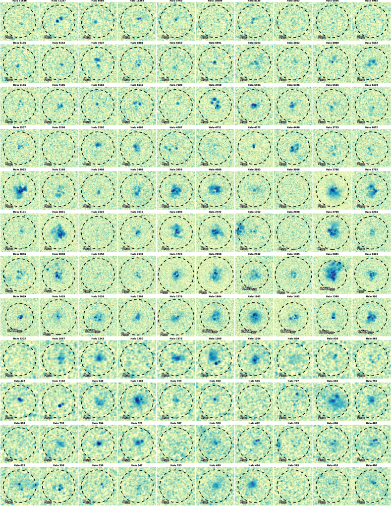
Figure 18: Stacked O VII(f) and O VIII images of the Simba galaxy halos.

Tables 2, 3, and 4 list all the simulated galaxy halos that are used for the line surface brightness profiles, the line ratios, and the azimuthal substructure test. As described in section 2.2, we use three simulation suits, TNG100, EAGLE (100 Mpc box) and Simba (100 Mpc box), and subselect from each 120 galaxies. These galaxies are equally divided into a low mass sample $\log_{10}M_{200}/M_{\odot}=11.5-12$, a medium mass sample $\log_{10}M_{200}/M_{\odot}=12-12.5$, and a high mass sample $\log_{10}M_{200}/M_{\odot}=12.5-13$. In Figs. 16, 17, and 18, we show stacked O VII and  OVIII images for each of the galaxies, including instrumental background, foreground emission, and CXB (see section 2).

Table 2: IllustrisTNG halos

Halo	M⋆	M200	MBH	SFR	R500		Halo	M⋆	M500	MBH	SFR	R500
	$\mathrm{1}\mathrm{0}^{10}\mathrm{M}_{\odot}$	$\mathrm{1}\mathrm{0}^{12}\mathrm{M}_{\odot}$	$\mathrm{1}\mathrm{0}^{8}\mathrm{M}_{\odot}$	$\mathrm{M}_{\odot}\,\mathrm{y}\mathrm{r}^{-1}$	kpc			$\mathrm{1}\mathrm{0}^{10}\mathrm{M}_{\odot}$	$\mathrm{1}\mathrm{0}^{12}\mathrm{M}_{\odot}$	$\mathrm{1}\mathrm{0}^{8}\mathrm{M}_{\odot}$	$\mathrm{M}_{\odot}\,\mathrm{y}\mathrm{r}^{-1}$	kpc
TNG100 low mass sample
582879	0.63	0.33	0.32	0.487	99		541402	1.27	0.64	0.54	1.189	123
539812	1.56	0.63	0.62	0.418	125		581475	1.71	0.34	0.86	0.076	102
513718	3.71	0.95	1.25	2.564	142		530171	0.98	0.75	0.22	1.217	125
509402	3.21	0.96	1.08	0.507	142		489863	1.99	0.99	0.79	4.143	130
505030	2.49	0.84	0.54	2.334	138		513262	3.98	0.97	1.89	0.000	142
557923	1.31	0.49	0.34	1.372	114		512631	0.44	0.93	0.19	0.667	143
562983	0.29	0.38	0.09	0.466	94		509468	4.90	0.96	1.01	4.559	144
551694	1.04	0.49	0.41	0.967	111		567124	1.01	0.47	0.57	1.141	113
537893	1.24	0.44	0.53	1.357	110		525081	1.77	0.84	0.88	6.793	135
524295	2.99	0.82	0.98	2.155	135		539998	2.16	0.66	1.01	0.534	127
562544	0.52	0.51	0.23	0.479	116		528531	1.43	0.86	0.81	1.569	141
555033	0.77	0.37	0.36	0.623	103		554843	0.41	0.50	0.13	0.402	109
556431	2.02	0.61	1.35	0.000	122		505616	4.03	0.98	1.66	0.000	145
538080	3.26	0.70	1.35	0.000	129		523231	2.35	0.81	0.78	1.281	135
559158	1.43	0.45	0.50	1.081	106		558021	1.10	0.52	0.32	1.231	116
520230	1.68	0.73	0.53	0.885	130		465921	0.91	0.78	0.39	1.842	127
506526	2.07	0.89	1.17	1.163	134		505680	0.34	0.38	0.08	0.403	87
578707	0.43	0.34	0.30	0.449	99		567178	1.42	0.44	0.29	1.512	112
589067	1.00	0.35	0.59	0.306	103		567085	0.63	0.41	0.22	0.970	107
547892	1.76	0.58	1.06	1.285	121		549236	0.67	0.50	0.31	0.774	110
TNG100 medium mass halos
497646	4.90	1.09	0.91	2.781	149		497800	4.45	1.20	1.56	0.000	156
487244	6.27	1.20	1.56	2.622	155		490577	6.15	1.30	1.50	0.005	160
421835	7.19	3.10	1.69	0.177	208		419061	3.76	1.92	1.01	5.303	164
460273	6.27	1.79	2.39	0.005	175		484427	5.20	1.38	1.90	0.000	157
422831	6.59	2.97	2.70	0.000	203		449034	8.66	2.34	2.75	0.000	189
411321	6.72	1.93	1.80	0.479	172		449549	7.59	2.24	2.28	0.000	189
428813	6.57	2.70	1.75	0.002	199		442855	7.61	2.24	2.47	0.001	188
483900	5.75	1.31	1.61	0.718	159		460746	8.07	1.86	2.49	0.015	174
444545	5.25	2.79	3.56	0.000	200		438996	5.76	1.78	2.60	0.000	172
463453	5.26	1.59	1.89	0.000	163		494771	4.13	1.11	1.04	3.695	149
461136	6.04	1.80	1.81	0.117	177		493920	5.39	1.40	2.56	0.000	162
432711	8.37	2.67	2.62	0.649	198		471801	4.27	1.32	1.83	0.000	155
418230	8.11	2.42	1.61	0.019	192		428158	7.14	2.95	3.57	0.000	207
448269	5.25	2.03	1.86	1.907	174		433537	4.76	2.65	3.24	0.000	196
459270	4.32	2.14	2.95	0.000	187		426764	8.91	2.39	2.65	0.248	187
462391	4.59	1.90	2.11	0.000	175		460823	5.29	1.98	2.19	0.000	179
436233	5.18	2.63	2.75	0.000	196		456014	4.82	2.04	1.70	0.000	173
432831	5.17	2.97	3.41	0.000	206		480587	5.02	1.43	2.23	0.000	161
426483	10.13	2.88	3.15	0.002	205		471109	6.03	1.50	1.47	0.021	164
458378	6.63	2.19	2.72	0.000	184		469930	7.65	1.51	1.58	1.236	166
TNG100 high mass halos
390859	8.48	4.75	4.49	0.000	237		415373	9.43	3.66	4.95	0.000	219
383307	10.31	4.87	4.52	0.365	232		332068	8.15	5.34	2.78	0.034	217
387236	12.15	4.46	3.65	0.865	230		341356	11.92	7.18	5.27	0.064	273
377398	17.08	6.09	5.98	0.003	260		414447	8.42	3.44	3.35	0.000	211
333672	10.32	8.70	2.34	0.472	288		312412	13.09	7.79	4.97	0.000	282
394439	12.03	4.29	3.39	1.286	230		399520	8.74	3.93	4.83	0.000	220
249164	13.77	9.95	6.87	0.069	298		372568	13.64	5.53	5.60	0.104	254
413091	12.81	3.67	2.39	0.021	218		342689	13.01	4.74	3.69	0.201	238
346420	11.97	5.31	5.37	0.056	244		359639	14.99	6.41	7.83	0.456	261
360916	5.75	5.98	4.77	0.000	238		405460	12.18	3.23	5.59	0.000	206
345812	10.51	8.82	3.41	5.729	295		288014	7.10	9.55	2.24	0.246	292
384103	6.69	4.91	2.94	0.010	218		339547	11.91	7.57	4.71	0.000	271
359086	8.14	7.75	4.70	0.000	283		382059	11.56	3.80	2.87	2.505	221
377212	14.52	5.98	7.86	0.079	258		376132	7.35	3.61	4.06	0.000	214
337444	10.97	7.94	6.50	0.000	278		329105	14.29	8.71	8.22	1.058	294
361418	6.22	6.46	4.64	0.000	252		399969	11.73	4.23	4.43	0.000	227
313402	10.00	9.02	6.59	0.002	245		386429	9.24	4.78	1.69	4.350	208
327822	10.97	4.27	2.22	4.068	222		371859	8.90	5.62	7.07	0.000	253
298206	12.79	8.75	5.82	1.032	282		398110	11.38	4.01	4.98	0.033	230
312891	15.21	9.78	11.30	0.088	303		380119	12.16	4.85	5.02	0.290	239
TNG50 halos
358608	15.06	5.04	4.38	4.018	243		467415	8.68	2.08	2.13	9.224	183

Table 3: EAGLE halos

Halo	M⋆	M200	MBH	SFR	R500		Halo	M⋆	M500	MBH	SFR	R500
	$\mathrm{1}\mathrm{0}^{10}\mathrm{M}_{\odot}$	$\mathrm{1}\mathrm{0}^{12}\mathrm{M}_{\odot}$	$\mathrm{1}\mathrm{0}^{8}\mathrm{M}_{\odot}$	$\mathrm{M}_{\odot}\,\mathrm{y}\mathrm{r}^{-1}$	kpc			$\mathrm{1}\mathrm{0}^{10}\mathrm{M}_{\odot}$	$\mathrm{1}\mathrm{0}^{12}\mathrm{M}_{\odot}$	$\mathrm{1}\mathrm{0}^{8}\mathrm{M}_{\odot}$	$\mathrm{M}_{\odot}\,\mathrm{y}\mathrm{r}^{-1}$	kpc
low mass sample
2703	0.45	0.42	0.02	0.691	104		2144	0.79	0.44	0.01	0.292	110
2258	0.27	0.52	0.02	0.477	109		2824	0.66	0.44	0.01	0.431	109
2577	0.21	0.37	0.00	0.498	95		1949	1.15	0.69	0.02	1.131	125
2578	1.15	0.52	0.01	0.480	117		1791	0.99	0.86	0.05	0.606	139
2044	1.07	0.71	0.01	0.190	117		2478	0.53	0.39	0.02	0.306	104
2535	0.71	0.51	0.02	0.614	114		2370	0.92	0.55	0.02	0.992	117
1662	1.32	0.85	0.07	1.099	133		2428	0.41	0.33	0.01	0.411	98
2899	0.40	0.38	0.01	0.750	98		2726	0.71	0.53	0.08	0.000	119
2592	1.14	0.50	0.05	0.205	115		1730	2.86	0.78	0.05	1.402	132
2345	0.36	0.53	0.01	0.230	117		2864	0.56	0.41	0.01	0.355	105
2557	0.28	0.37	0.02	0.326	98		2516	0.83	0.48	0.03	0.434	113
2671	0.25	0.48	0.01	0.408	100		1725	1.93	0.81	0.11	0.003	131
2118	0.85	0.39	0.01	0.823	105		2902	0.36	0.38	0.01	0.241	97
1647	2.13	0.87	0.08	0.577	138		2874	0.31	0.39	0.02	0.147	105
2184	1.47	0.65	0.03	0.690	125		1803	1.64	0.73	0.03	1.379	128
1581	1.21	0.82	0.12	0.018	123		2688	0.73	0.52	0.04	0.338	115
2176	1.09	0.68	0.01	0.547	124		2338	0.29	0.63	0.03	0.304	125
1564	2.37	0.92	0.07	0.885	140		2852	0.63	0.46	0.04	0.578	112
2716	0.56	0.42	0.01	0.478	100		1569	1.50	0.84	0.03	0.983	132
2066	1.59	0.69	0.05	0.768	126		2157	1.43	0.59	0.05	1.220	121
medium mass halos
1096	2.81	1.45	0.28	0.111	160		798	4.79	1.67	0.31	0.010	162
700	4.45	2.70	0.81	1.100	201		816	4.28	1.86	0.07	2.487	170
521	2.76	2.19	0.73	0.255	185		1256	1.61	1.20	0.04	0.776	155
480	6.90	3.12	0.76	0.218	203		1303	1.44	1.27	0.06	0.632	156
964	4.46	1.55	0.04	2.218	166		846	2.02	1.82	0.23	0.041	164
789	2.47	2.19	0.47	0.000	189		1233	2.02	1.06	0.10	0.548	144
1244	2.56	1.10	0.27	1.034	147		774	4.40	2.20	0.53	0.021	185
965	2.84	1.53	0.28	0.577	158		1133	3.28	1.28	0.16	1.896	153
1350	2.59	1.05	0.15	1.869	147		1296	3.15	1.09	0.26	0.910	149
927	5.02	1.83	0.49	1.128	179		833	5.81	2.03	0.79	2.467	182
482	4.98	2.67	0.58	1.394	198		660	5.16	2.23	0.14	7.143	183
744	3.43	2.06	0.72	0.053	183		1122	3.16	1.51	0.31	0.500	165
1205	2.47	1.06	0.19	1.044	144		597	4.57	3.01	0.48	2.220	203
933	3.30	1.74	0.52	0.000	170		977	3.68	1.63	0.30	1.095	168
527	4.90	2.92	0.80	2.603	196		914	2.22	1.53	0.02	3.448	164
1142	2.33	1.25	0.49	0.024	155		961	1.82	1.69	0.39	0.000	168
1117	3.30	1.32	0.13	2.053	155		835	3.91	1.79	0.08	2.951	173
512	4.32	2.70	0.39	2.959	196		622	3.81	3.03	0.41	1.113	207
621	4.63	2.41	0.10	2.462	177		689	2.65	2.14	0.27	0.412	175
709	3.29	2.35	0.24	1.544	178		577	4.82	2.42	0.45	1.189	181
high mass halos
207	8.57	4.86	0.34	6.738	223		218	6.27	7.19	1.27	0.533	261
214	12.05	8.57	2.52	0.101	294		262	8.67	6.05	1.67	0.094	255
209	9.18	8.53	2.77	2.621	287		541	8.47	3.29	1.22	1.588	210
235	7.45	6.75	1.71	3.997	264		399	5.15	3.89	2.18	0.000	226
251	9.04	6.17	2.02	3.160	252		342	4.51	3.89	1.20	0.199	224
253	9.42	6.85	1.34	4.110	262		132	11.83	6.70	1.35	1.723	255
244	8.89	6.58	0.89	4.195	255		169	7.16	9.12	0.68	4.680	256
377	9.35	4.19	0.85	0.538	222		224	5.07	4.59	1.44	2.278	236
283	6.32	5.87	1.17	3.746	252		231	13.12	7.43	2.13	0.000	271
208	8.55	3.93	1.21	0.000	226		422	6.10	4.14	0.91	1.463	230
282	3.92	5.62	0.27	2.259	219		141	12.53	8.53	2.14	4.794	285
189	12.05	7.94	4.10	0.124	275		121	9.44	9.98	2.75	1.904	298
248	4.91	5.62	2.34	0.081	247		439	6.53	3.58	0.66	3.127	212
151	13.37	9.33	2.03	4.601	285		203	9.59	4.32	1.53	1.344	229
194	11.61	8.99	1.71	3.159	277		360	8.57	4.95	1.52	0.008	240
539	6.25	3.24	1.01	0.019	210		177	8.83	9.25	2.88	2.211	292
427	6.19	4.05	0.79	0.765	223		254	11.07	7.55	1.64	0.385	274
334	8.81	5.09	1.80	0.000	240		243	7.60	7.78	0.21	0.124	277
408	6.70	4.39	0.30	3.627	227		277	3.39	4.65	0.43	1.054	212
276	8.18	4.37	1.13	0.104	221		337	8.00	5.22	1.60	0.793	235

Table 4: Simba halos

Halo	M⋆	M200	MBH	SFR	R500		Halo	M⋆	M500	MBH	SFR	R500
	$\mathrm{1}\mathrm{0}^{10}\mathrm{M}_{\odot}$	$\mathrm{1}\mathrm{0}^{12}\mathrm{M}_{\odot}$	$\mathrm{1}\mathrm{0}^{8}\mathrm{M}_{\odot}$	$\mathrm{M}_{\odot}\,\mathrm{y}\mathrm{r}^{-1}$	kpc			$\mathrm{1}\mathrm{0}^{10}\mathrm{M}_{\odot}$	$\mathrm{1}\mathrm{0}^{12}\mathrm{M}_{\odot}$	$\mathrm{1}\mathrm{0}^{8}\mathrm{M}_{\odot}$	$\mathrm{M}_{\odot}\,\mathrm{y}\mathrm{r}^{-1}$	kpc
low mass sample
4721	1.94	0.93	0.51	1.702	140		6326	1.38	0.68	0.28	2.072	126
5266	0.63	0.75	0.04	1.432	128		4496	1.43	0.94	0.16	4.941	133
7185	1.60	0.58	0.24	1.664	121		6991	1.10	0.50	0.20	1.610	109
3729	1.68	0.97	0.43	2.214	124		5205	2.40	0.83	0.12	2.447	136
7837	0.91	0.49	0.17	2.523	113		4172	1.34	0.93	0.38	1.880	135
5566	1.74	0.60	0.49	1.522	119		11638	0.83	0.32	0.05	1.070	98
6542	1.42	0.60	0.37	1.558	122		4862	1.65	0.53	0.38	1.122	119
6652	1.18	0.50	0.26	2.086	111		5494	2.18	0.65	0.57	1.301	123
7552	1.63	0.58	0.27	1.385	119		4267	0.92	0.92	0.34	2.029	132
9143	0.87	0.47	0.09	1.036	111		6156	0.87	0.58	0.04	5.991	116
7189	0.85	0.62	0.14	1.226	115		3768	1.89	0.64	0.46	3.384	119
5263	2.38	0.51	0.56	3.635	113		5762	1.15	0.36	0.33	2.065	104
8135	0.83	0.38	0.16	1.581	103		4965	0.30	0.40	0.29	2.137	107
4672	0.95	0.97	0.24	1.679	140		5557	1.31	0.75	0.28	1.001	130
6084	1.18	0.35	0.18	2.453	100		9136	1.11	0.43	0.22	1.063	107
11327	1.04	0.33	0.24	1.031	101		6800	1.06	0.54	0.14	1.076	116
5936	0.93	0.39	0.21	2.142	102		8881	0.82	0.50	0.08	1.207	116
4439	1.65	0.73	0.47	1.755	126		11362	0.69	0.35	0.10	1.166	100
10409	0.70	0.37	0.11	1.507	103		5802	1.31	0.38	0.37	1.842	104
4802	3.35	0.91	0.44	4.681	141		5565	1.33	0.70	0.21	1.498	124
medium mass halos
2788	7.33	1.34	0.87	5.462	158		2992	5.23	1.06	0.40	15.196	148
2722	4.66	1.55	0.93	10.480	159		2401	4.21	1.12	1.10	1.439	151
1323	6.02	2.22	0.96	3.030	170		1792	3.99	1.38	0.21	11.855	147
3956	4.32	1.13	0.40	5.601	150		1864	11.30	2.48	1.17	3.974	195
1278	7.51	2.37	1.30	2.963	180		2496	2.55	1.49	0.23	9.434	156
2132	11.38	2.12	0.77	4.576	188		1650	2.30	1.84	1.38	1.849	170
2030	4.23	1.79	0.49	4.188	160		2166	2.76	1.08	0.42	5.268	146
395	8.61	3.13	3.03	3.697	206		1201	6.09	2.33	1.25	1.188	180
2828	4.97	1.57	1.19	5.388	167		2622	2.52	1.47	0.99	1.495	157
2058	6.82	2.03	0.99	5.198	183		1380	6.64	3.13	0.61	1.297	209
2131	3.20	1.92	0.88	1.257	172		2089	6.11	2.23	1.74	1.040	186
4086	4.22	1.15	0.15	6.362	152		3606	5.71	1.23	1.43	2.548	154
1403	3.92	2.24	0.90	3.556	176		1726	7.23	1.99	2.01	6.853	179
1985	7.44	2.13	0.67	1.127	183		2081	5.61	2.19	0.40	9.351	191
1482	6.83	2.86	1.91	3.100	197		1942	15.99	2.56	0.63	5.588	199
2204	3.86	1.59	0.48	1.382	164		2790	5.33	1.58	0.29	14.680	168
3101	6.34	1.45	0.36	9.689	163		3409	3.16	1.12	1.04	2.281	148
1762	2.39	1.57	0.79	4.764	154		3012	4.14	1.49	1.02	3.209	163
2831	3.98	1.45	0.16	13.514	152		2036	10.33	2.31	1.31	5.877	193
2066	1.14	1.65	0.24	3.519	144		3883	8.74	1.22	0.55	1.652	158
high mass halos
793	11.00	5.82	1.25	5.868	236		483	7.07	7.41	2.06	1.367	241
414	11.41	9.12	9.96	7.806	296		928	5.38	3.69	1.77	2.034	201
343	17.38	9.31	8.13	1.533	292		406	17.12	9.79	4.20	6.775	300
704	15.05	6.15	2.46	1.044	259		859	19.38	3.63	2.00	8.954	209
550	5.75	6.84	2.71	2.130	256		729	11.17	4.49	3.22	2.392	236
589	8.08	5.37	4.71	1.272	234		499	9.01	8.77	2.22	2.046	280
1101	13.65	4.24	1.20	5.909	231		533	9.96	8.53	4.88	1.674	283
606	8.68	7.33	1.81	1.538	276		576	6.72	4.69	4.46	3.734	233
797	5.25	5.10	3.96	2.142	242		981	19.67	3.73	2.51	1.825	220
587	6.22	6.79	3.92	5.185	244		530	10.34	7.74	7.76	1.340	259
422	6.25	3.88	3.30	7.754	204		792	4.40	5.33	2.31	1.513	242
1162	9.05	3.98	1.35	1.839	214		1250	5.21	3.48	2.66	1.492	195
675	6.11	7.43	3.49	1.278	269		303	10.63	7.19	4.63	4.744	267
663	5.61	5.19	2.86	3.604	239		521	9.28	6.21	1.21	4.473	200
647	10.31	7.93	4.45	1.167	283		1369	3.15	3.58	1.66	9.063	217
1302	4.14	3.16	1.78	2.846	202		1375	4.02	3.56	0.83	4.062	219
1264	11.70	3.60	0.96	4.972	218		930	5.35	4.52	0.83	3.742	226
410	9.51	9.42	4.18	1.048	303		1067	5.37	3.26	2.46	2.147	201
948	4.69	4.21	3.68	3.268	229		396	13.91	7.52	5.18	1.300	263
472	7.78	7.03	3.55	2.297	257		1343	11.42	3.41	0.34	1.601	216

References

- Al-Baidhany et al. (2020) Al-Baidhany, I. A., Chiad, S. S., Jabbar, W. A., et al. 2020, in INTERNATIONAL CONFERENCE OF NUMERICAL ANALYSIS AND APPLIED MATHEMATICS ICNAAM 2019 (AIP Publishing)
- Anders & Grevesse (1989) Anders, E., & Grevesse, N. 1989, Geochim. Cosmochim. Acta, 53, 197
- Anderson & Bregman (2011) Anderson, M. E., & Bregman, J. N. 2011, Astrophys. J., 737, 22
- Anderson et al. (2015) Anderson, M. E., Churazov, E., & Bregman, J. N. 2015, Mon. Not. R. Astron. Soc., 455, 227
- Arnaud (1996) Arnaud, K. A. 1996, in Astronomical Society of the Pacific Conference Series, Vol. 101, Astronomical Data Analysis Software and Systems V, ed. G. H. Jacoby & J. Barnes, 17
- Ayromlou et al. (2022) Ayromlou, M., Nelson, D., & Pillepich, A. 2022, arXiv e-prints, arXiv:2211.07659
- Barret et al. (2013) Barret, D., den Herder, J. W., Piro, L., et al. 2013. https://arxiv.org/abs/1308.6784
- Barret et al. (2018) Barret, D., Trong, T. L., den Herder, J.-W., et al. 2018, in Space Telescopes and Instrumentation 2018: Ultraviolet to Gamma Ray, Vol. 10699 (SPIE), 324–338
- Barret et al. (2023) Barret, D., Albouys, V., Herder, J.-W. d., et al. 2023, Exp. Astron., 55, 373
- Behroozi et al. (2019) Behroozi, P., Wechsler, R. H., Hearin, A. P., & Conroy, C. 2019, Mon. Not. R. Astron. Soc., 488, 3143
- Behroozi et al. (2010) Behroozi, P. S., Conroy, C., & Wechsler, R. H. 2010, Astrophys. J., 717, 379
- Benson et al. (2000) Benson, A. J., Bower, R. G., Frenk, C. S., & White, S. D. M. 2000, Mon. Not. R. Astron. Soc., 314, 557
- Bluem et al. (2022) Bluem, J., Kaaret, P., Kuntz, K. D., et al. 2022, ApJ, 936, 72
- Bogdán et al. (2017) Bogdán, Á., Bourdin, H., Forman, W. R., et al. 2017, Astrophys. J., 850, 98
- Bogdán et al. (2013a) Bogdán, Á., Forman, W. R., Kraft, R. P., & Jones, C. 2013a, Astrophys. J., 772, 98
- Bogdán & Gilfanov (2011) Bogdán, Á., & Gilfanov, M. 2011, Mon. Not. R. Astron. Soc., 418, 1901
- Bogdán et al. (2013b) Bogdán, Á., Forman, W. R., Vogelsberger, M., et al. 2013b, Astrophys. J., 772, 97
- Bogdán et al. (2015) Bogdán, Á., Vogelsberger, M., Kraft, R. P., et al. 2015, Astrophys. J., 804, 72
- Bogdan et al. (2023) Bogdan, A., Khabibullin, I., Kovacs, O., et al. 2023, arXiv e-prints, arXiv:2306.05449
- Bregman et al. (2022) Bregman, J. N., Hodges-Kluck, E., Qu, Z., et al. 2022, ApJ, 928, 14
- Burke et al. (2020) Burke, D., Laurino, O., Wmclaugh, et al. 2020, sherpa/sherpa: Sherpa 4.12.1
- Byrohl & Nelson (2022) Byrohl, C., & Nelson, D. 2022, arXiv e-prints, arXiv:2212.08666
- Carlesi et al. (2022) Carlesi, E., Hoffman, Y., & Libeskind, N. I. 2022, Mon. Not. R. Astron. Soc., 513, 2385
- Carr et al. (2023) Carr, C., Bryan, G. L., Fielding, D. B., Pandya, V., & Somerville, R. S. 2023, ApJ, 949, 21
- Cash (1979) Cash, W. 1979, Astrophys. J., 228, 939
- Cen & Ostriker (1999) Cen, R., & Ostriker, J. P. 1999, ApJ, 514, 1
- Cen & Ostriker (2000) —. 2000, ApJ, 538, 83