The Atacama Cosmology Telescope: High-resolution component-separated maps across one-third of the sky

Abstract

Observations of the millimeter sky contain valuable information on a number of signals, including the blackbody cosmic microwave background (CMB), Galactic emissions, and the Compton-$y$ distortion due to the thermal Sunyaev-Zel’dovich (tSZ) effect. Extracting new insight into cosmological and astrophysical questions often requires combining multi-wavelength observations to spectrally isolate one component. In this work, we present a new arcminute-resolution Compton-$y$ map, which traces out the line-of-sight-integrated electron pressure, as well as maps of the CMB in intensity and E-mode polarization, across a third of the sky (around 13,000 sq. deg.). We produce these through a joint analysis of data from the Atacama Cosmology Telescope (ACT) Data Release 4 and 6 at frequencies of roughly 93, 148, and 225 GHz, together with data from the Planck satellite at frequencies between 30 GHz and 545 GHz. We present detailed verification of an internal linear combination pipeline implemented in a needlet frame that allows us to efficiently suppress Galactic contamination and account for spatial variations in the ACT instrument noise. These maps provide a significant advance, in noise levels and resolution, over the existing Planck component-separated maps and will enable a host of science goals including studies of cluster and galaxy astrophysics, inferences of the cosmic velocity field, primordial non-Gaussianity searches, and gravitational lensing reconstruction of the CMB.

I Introduction

Millimeter observations of the sky provide a window into the universe across cosmic history as they comprise signals from our solar system (Naess et al., 2021), our Galaxy (Baxter et al., 2018; Planck Collaboration Int. XXXIV, 2016; Planck Collaboration Int. XVIII, 2015; Planck Collaboration Int. XLIV, 2016), galaxy clusters (Sunyaev and Zeldovich, 1972; Sunyaev and Zeldovich, 1980a; Staniszewski et al., 2009; Planck Collaboration XXII, 2016; Hasselfield et al., 2013; Bleem et al., 2015), high-redshift star-forming galaxies (Planck Collaboration XXX, 2014), the cosmic microwave background (CMB) (Penzias and Wilson, 1965; Fixsen et al., 1996; Hinshaw et al., 2013; Dutcher et al., 2021; Aiola et al., 2020), and more. This profusion of signals makes these observations well suited for learning about astrophysical and cosmological processes. However, it also comes at a cost: the information from any given process is mixed with the multitude of other signatures. Sources of noise and instrumental effects further complicate these measurements. Though there are times when it may be best to deal directly with the unprocessed data sets (for instance in the analysis of the power spectrum of the primary CMB anisotropies) for many science cases it is beneficial to isolate a component of interest from others; collectively, methods to address this task are known as component separation techniques. Through these methods, we can produce sky maps of components of interest with reduced contamination from the other sky signals, thereby enabling detailed studies of the relevant physical processes.

Component separation methods can be roughly divided into two categories: blind and unblind methods. In the prototypical unblind approach, a model of the sky is developed and parameters describing the scale and/or spatial and frequency dependence of the components of the sky is fit to the data; an example of this is the commander method used in Planck and BeyondPlanck (Eriksen et al., 2006, 2008; Galloway et al., 2022). On the other hand, blind methods make minimal assumptions about the contributions to the observations, with the simplest methods only assuming that the frequency dependence of the component of interest is known, and focus on using the empirical properties of the data. Blind and semi-blind approaches include fastica, sevem, smica, gnilc, and milca (Maino et al., 2002; Fernández-Cobos et al., 2012; Cardoso et al., 2008; Remazeilles et al., 2011a; Hurier et al., 2013). These approaches each have their merits; blind approaches are typically highly flexible, simple, and fast, whilst unblind approaches can provide complete models of the sky and easily include complex priors (see e.g., Delabrouille and Cardoso, 2007; Leach et al., 2008, for a comparison of these approaches).

In this work we use a blind method, known as the internal linear combination (ILC) method. Since the first application of the ILC method to the COBE data by Ref. (Bennett et al., 1992), this method has been extensively used in the analysis of CMB data, including data from WMAP, Planck, the Atacama Cosmology Telescope (ACT), and South Pole Telescope (SPT) experiments (Bennett et al., 2003; Delabrouille et al., 2009; Planck Collaboration XXII, 2016; Madhavacheril et al., 2020; Aghanim et al., 2019; Bleem et al., 2022). The main benefits of the ILC approach are its simplicity, minimal assumptions, and flexibility. The ILC method can be applied to data in many different domains, e.g., real space, harmonic space, or a wavelet frame — as in this work. Wavelet frames provide joint localization in real and harmonic space. Wavelets are thus well suited to analyzing CMB data where extragalactic signals are best described in the harmonic basis, and Galactic and some instrumental effects are better described in pixel space. Wavelets were first combined with ILC methods in (Delabrouille et al., 2009) and have since been further developed and applied to Planck data (Remazeilles et al., 2011a; Remazeilles et al., 2013; Hurier et al., 2013; Planck Collaboration IV, 2020). Our implementation follows that developed in Ref. (Remazeilles et al., 2013), with a key modification: a new method to mitigate the “ILC bias”. The “ILC bias” arises as the weights used to linearly combine the individual frequency maps are obtained from the data themselves. Our mitigation method works by ensuring that these empirically determined weights are never applied to the same data from which they were estimated.

We focus on studying two sky signals: (i) the thermal Sunyaev-Zel’dovich (tSZ) effect and (ii) the blackbody component in temperature and polarization. The latter blackbody component includes the lensed CMB in temperature and polarization and the kinetic Sunyaev-Zel’dovich (kSZ) effect in temperature. The Compton-$y$ signal, sourced by the tSZ effect (Sunyaev and Zeldovich, 1972; Sunyaev and Zeldovich, 1980b), is an important cosmological and astrophysical probe as it traces the distribution of free electrons, from hot ionized matter, throughout the universe. Isolating this signal from the dominant foreground signals is essential for studies as diverse as constraints on massive neutrinos or on cluster feedback processes (Madhavacheril et al., 2017; Pandey et al., 2019; Amodeo et al., 2021). Component-separated, or cleaned, blackbody temperature maps are needed for a diverse range of studies including CMB lensing and primordial non-Gaussianity analyses (van Engelen et al., 2014; Osborne et al., 2014; Hill, 2018; Coulton et al., 2022), where it is important to remove contaminant signals from Galactic and extragalactic sources to avoid biased inferences, and analyses of the kSZ effect (Sunyaev and Zeldovich, 1980a), where other extragalactic signals can bias measurements of cosmic gas distributions and act as large sources of noise (Hill et al., 2016; Schaan et al., 2021).

In this work we apply this pipeline to new data from the upcoming ACT Data Release 6 (DR6) and previous data from ACT Data Release 4 (DR4) and the Planck satellite (Fowler et al., 2007; Planck Collaboration I, 2020). The Planck satellite’s precise measurements of the large scale millimeter sky ($\gtrsim 5^{\prime}$) naturally complements ACT’s high resolution measurements ($\sim 1.5^{\prime}$). The main results of this work are $1.6^{\prime}$ resolution maps of the tSZ, CMB temperature, and CMB E-mode polarization anisotropies, with mean white noise levels of $\sim 15\,\mu$K-arcmin in temperature. These products build on existing component-separated maps from Planck (Planck Collaboration XII, 2014; Planck Collaboration IX, 2016; Planck Collaboration X, 2016; Planck Collaboration IV, 2020) by utilizing the high-resolution ACT data to provide improved small-scale information. This is achieved at the cost of limiting the maps to the $\sim 1/3$ of the sky observed by ACT. However, our new maps cover $\sim 5\times$ larger sky fractions than existing high-resolution component-separated maps, such as those from Ref. (Madhavacheril et al., 2020) and Ref. (Bleem et al., 2022). Further, our use of the wavelet frame is complementary to the harmonic and Fourier space method (see e.g., Atkins et al., 2023, for a discussion of some tradeoffs of these frames) used in Ref. (Madhavacheril et al., 2020) and Ref. (Bleem et al., 2022) and allows for a better removal of Galactic foregrounds.

The products of this work — including maps with $0.5^{\prime}$ pixels, simulations, and auxiliary data — will be made available on LAMBDA and NERSC. This paper is part of a suite of ACT DR6 papers, which will include a dedicated paper describing the single-frequency maps.

This paper is structured as follows: in Section II we briefly describe the data used in this paper and in Section III we provide the details of our component separation pipeline. We present the component-separated maps in Section IV and discuss a few of their key properties in Section V. We then conclude in Section VI. In Appendix A we describe the simulations used to validate our tools and simulated products that accompany this work and in Appendix B we describe the harmonic ILC method used as a baseline, comparison method. In Appendix C we provide a detailed description of the ILC bias reduction method. Finally in Appendix D we describe how we include instrumental systematic effects into our analysis pipeline.

II Data Sets

The single frequency maps used in this work are from the ACT DR4 and upcoming DR6 data sets and the Planck NPIPE analysis. Tables 1 and 2 provide summaries of the key properties of the ACT and Planck data sets, respectively.

The Atacama Cosmology Telescope was a 6 m off-axis Gregorian telescope (Fowler et al., 2007) located at an elevation of 5190 m in the Atacama Desert of Chile, used to measure the CMB from 2007 to 2022 (e.g., Dünner et al., 2013; Dunkley et al., 2011; Das et al., 2011; Sievers et al., 2013; Gralla et al., 2020a; Louis et al., 2017a; Naess et al., 2014; Aiola et al., 2020; Naess et al., 2020). The DR4 and DR6 data comprise multifrequency observations across $\sim 1/3$ of the sky, measured by polarization-sensitive arrays of feedhorn-coupled transition-edge sensor (TES) bolometers (Grace et al., 2014; Datta et al., 2014; Ho et al., 2016; Henderson et al., 2016; Ho et al., 2017; Choi et al., 2018; Li et al., 2018). The arrays were cooled to 100 mK in a receiver providing separate optics chains (lenses and filters) for each array (Thornton et al., 2016). We label the detectors according to the approximate centers of their frequency responses in GHz as follows: f090, f150, and f220. The ACT maps are produced in the Plate-Carrée (hereafter abbreviated CAR) projection scheme. This scheme is used for both the input maps and the needlet maps. The CAR maps have a rectangular pixelization with the $x$ and $y$ axes aligned with right ascension and declination, respectively.

The ACT DR4 data cover night-time ACT observations over four observing seasons from 2013 to 2016 (Aiola et al., 2020; Choi et al., 2020). The DR4 data set comprises a set of deep observations in the regions labeled by “D5”, “D6”, “D56”, “D1”, “D8”, and “BN” in Fig. 1, as well as shallower observations of the “wide” region. In this work, we only use the deep observations from DR4 as the noise levels in its wide field maps are too large to provide noticeable improvements in our analysis. The DR4 data were collected by the three arrays of the ACTPol camera Thornton et al. (2016). The first two arrays, called PA1 and PA2 (where PA is an abbreviation for Polarimeter Array), were sensitive to the f$150$ band (124–172 GHz) whilst the third array was dichroic, observing in both the f$090$ (77–112 GHz) and f$150$ bands.

The DR6 data sets include observations from 2017 to 2022 at three frequency bands: f090, f150, and f220 (182–277 GHz). The observational program targeted the “wide” field. For this work, we use only the night-time portion of the data taken in the first five observing seasons, up to 2021. The Advanced ACT camera, used for these observations, was equipped with three dichroic arrays: PA4 at f$150$ and f$220$, and PA5 and PA6, each sensitive to both f$090$ and f$150$ (Henderson et al., 2016). Each frequency band of each array was mapped separately, but observations from different seasons were combined. Each of these data sets (i.e. the separate data from each frequency of each array) was further divided into eight sub-portions, hereafter referred to as “splits”, with independent instrumental and atmospheric noise. This analysis uses the first science-grade version of the ACT DR6 maps, labeled dr6.01. Since these single-frequency maps were generated, some refinements have been made to the ACT mapmaking that improve the large-scale transfer function and polarization noise levels. A second version of the input maps are expected to be used for further science analyses and for the DR6 public data release, and we will update the derived products as those maps are produced and released. More details of these maps will be provided in an upcoming paper.

In addition to the frequency maps, we used the DR4 and DR6 beams, point source catalogs, and passbands. The DR4 products are described in Ref. (Datta et al., 2019; Aiola et al., 2020; Gralla et al., 2020b; Lungu et al., 2022). The DR6 products are produced by similar methods, which will be detailed in an upcoming publication. In Appendix D we plot the DR6 passbands used in this work (Fig. 4 of Ref. (Madhavacheril et al., 2020) shows the DR4 passbands); these are key inputs for the component separation pipeline. The ACT point source catalogs are created for each frequency by applying a matched filter to a map obtained from combining the individual data splits (Stetson, 1987).

For the Planck data, we use the NPIPE maps described in (Planck Collaboration Int. LVII, 2020). These single-frequency maps cover the full sky, though we only use the data within the ACT “wide” footprint shown in Fig. 1. Planck has nine frequencies ranging from $30$ GHz to $857$ GHz, with resolutions ranging from 32 arcmin to 4.2 arcmin. The data are provided in two splits that are independently processed and largely statistically uncorrelated. Unlike the other frequencies, the Planck 857 GHz channel is not calibrated on the orbital dipole and instead uses a planetary absolute calibration. The challenges and uncertainties associated with this can impact the component separation; to avoid this, we do not use the 857 GHz data. In addition to the frequency maps, we use measurements of the Planck passbands (Zonca et al., 2009; Planck Collaboration II, 2014; Planck Collaboration IX, 2014; Hivon et al., 2017) and beams (Planck Collaboration IV, 2016; Planck Collaboration VII, 2016). We compare our results to component-separated maps produced by the Planck collaboration, specifically the MILCA Compton-$y$ map, and the Planck NILC Compton-$y$ and CMB maps (Planck Collaboration XXII, 2016; Hurier et al., 2013; Planck Collaboration IV, 2020).

Patch	Area	Frequency	Typical Depth	FWHM	Number of
Name	(deg2)	Band	($\mu$K arcmin)	(arcmin)	Data sets
Wide	$\sim 12200$	f090	20	2.1	2
Wide	$\sim 12200$	f150	20	1.4	3
Wide	$\sim 12200$	f220	65	1.0	1
D1	$\sim 60$	f150	15	1.4	1
D5	$\sim 60$	f150	12	1.4	1
D6	$\sim 60$	f150	10	1.4	1
D56	$\sim 560$	f150	20	1.4	5
D56	$\sim 560$	f090	17	2.0	1
BN	$\sim 1800$	f150	35	1.4	3
BN	$\sim 1800$	f090	33	2.0	1
D8	$\sim 200$	f150	25	1.4	3
D8	$\sim 200$	f090	20	2.0	1

Table 1: A summary of key properties of the ACT data set used in this analysis. The depth here refers to the white noise level and does not include atmospheric contributions, which are dominant at large scales. Note that the full-width half-maxima (FWHM) of the beams are from a Gaussian fit; however we use the full beam profiles in our analysis. In DR4 different observation seasons and different detector arrays were mapped separately. In DR6 different arrays and different frequencies were mapped separately, but all the observation seasons were combined. This leads to multiple data sets with similar footprints and noise levels, but different passbands and beams. The number of data sets for each patch is listed in the last column.

Reference	Frequency	Typical Depth	FWHM
Name	GHz	($\mu$K arcmin)	(arcmin)
P01	28.4	150	32
P02	44.1	162	28
P03	70.4	210	13
P04	100	77.4	9.7
P05	143	33	7.2
P06	217	46.8	4.9
P07	353	153	4.9
P08	545	1049	4.7

Table 2: A summary of key properties of the Planck data set used in this analysis, adapted from Table 4 of Ref. (Planck Collaboration I, 2020). The Planck maps cover the full sky and two splits are provided for each frequency. Note that the typical depths are approximate as we use the NPIPE Planck release, which has slightly lower white noise levels.

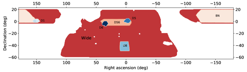
Figure 1: Footprints of the different data sets used in this work. ACT DR4 primarily focused on observing the deep patches, denoted by “D” and “BN”. Since 2016, ACT used upgraded detectors to observe significantly wider areas, denoted by “wide”, to approximately similar depth. We use the subset of Planck data that lies within this “wide” region. Note that the full ACT data set extends into the Galactic plane and in this work we adopt a smaller footprint to avoid contamination from bright Galactic emissions. The excised regions within the main footprint correspond to extended sources that are also masked or inpainted.

III Component Separation Pipeline

The component separation pipeline used in this work is composed of five main steps. We first outline these steps before describing the details of each stage in the remainder of this section.

1. Pre-processing: Before we can analyze the input frequency maps, we first perform a set of pre-processing steps. The aims of this step are: 1) to convolve the input maps to a common beam, 2) to filter the maps to remove contaminants such as scan-synchronous pickup, and 3) to remove bright sources, which can pose challenges to component separation and leave artifacts in the output maps. These steps are very similar to those performed in the lensing analysis, described in Ref. (Qu et al., 2023).

2. Needlet Decomposition: The next step is to transform the input maps into the wavelet frame. In this work we use the generalized “needlet” kernels (Narcowich et al., 2006; Guilloux et al., 2007); hence we refer to this frame as the needlet frame. The decomposition is achieved by convolving the input maps with the needlet kernels. This is implemented as a series of spherical harmonic transforms and filtering operations.

3. Component Separation: At each needlet scale we apply our component separation method — the needlet frame internal linear combination (NILC) method. This combines all the measurements at each needlet scale into a map of the component of interest. Using the methods developed in Ref. (Remazeilles et al., 2011b), we additionally generate maps of specific components that have other components removed (e.g., CMB temperature maps that are explicitly constructed to contain no tSZ anisotropies).

4. Inverse Needlet Decomposition: We then transform the ILC output from the needlet frame into the real-space basis. This is achieved by reconvolving the maps with the needlet kernels.

5. Correction for mode filtering: During the preprocessing of the ACT maps we apply a filtering step that removes a set of modes from the ACT maps. The aim is to remove modes contaminated by scan-synchronous pickup. Whilst this filtering step is not performed on the Planck maps, the absence of these modes in the ACT maps means they are partially missing from the output component-separated maps. To account for this we perform a final correction step. This step replaces the missing modes with those from a component-separated map formed from only the Planck maps.

III.1 Preprocessing

We preprocess the Planck and ACT maps in slightly different manners that are detailed below. The methodology for this closely follows that from Ref. (Aiola et al., 2020) and Ref. (Madhavacheril et al., 2020).

III.1.1 Planck preprocessing

We perform five preprocessing steps: first we project the Planck maps from their native HEALPix to CAR projection. Whilst the component separation pipeline does not require CAR maps, this step simplifies various preprocessing steps, such as the use of common masks. Next, we subtract sources from the two NPIPE splits at each frequency. For each data split we find the amplitudes of all point sources present in either the ACT or the Planck point source catalogs. As described in (Qu et al., 2023), the ACT catalogs are made by running a matched filter on a version of the Data Release 5 ACT+Planck maps (Naess et al., 2020) updated to use the new data in DR6, and objects detected at greater than $4\sigma$ are added to the catalog for each frequency band. We account for overlapping sources in this fit. We fit the amplitude to each data split to partially account for source variability (e.g., between the measured ACT flux and the brightness of the source in the Planck maps). We then select all the point sources whose amplitudes are detected at $>2\sigma$ in the Planck data and subtract a model of these from each input map. The model is given by the real-space beam profile scaled by the appropriate amplitude. Second, we mask the map; the mask we use for the Planck data is composed of three parts: a Galactic mask (the Planck 70% mask that masks the center of the Galaxy and leaves $70\%$ of the sky unmasked), a footprint mask that bounds the region observed by ACT, and a mask that removes bright extended sources from the maps, which otherwise can cause artifacts in an analogous manner to the point sources. We masked $\sim 20$ extended sources and we refer the reader to Ref. (Qu et al., 2023) for more details on the construction of the mask. We coadd the two splits in real space using an approximate inverse variance noise weighting, based on the per-pixel inverse variance maps.

The final preprocessing step is to transform the map to harmonic space and convolve the map to a common beam with a 1.6 arcmin full-width half-maximum (FWHM). We do this by applying an $\ell$-dependent weight given by the ratio of the harmonic transform of a 1.6 arcmin FWHM Gaussian beam to the harmonic transform of the NPIPE beams. The 1.6 arcmin FWHM is chosen to match the ACT resolution and is much smaller than the Planck FWHMs. This means that on small scales this ratio can become very large. To avoid numerical artifacts, and reduce the computational cost, we apply a small-scale cut that excludes scales where this ratio is $\gtrsim 50$. These scales are noise dominated and have no weight in the component separation pipeline. Thus, the results are insensitive to the specific value of this cut.

III.1.2 ACT preprocessing

The preprocessing of the ACT maps consists of five key steps: first, in a manner identical to the Planck maps, we subtract models for all the bright sources from the input map. The fit is performed for each split and, in this case, we remove all sources detected at or above 5$\sigma$. A lower threshold can be used for Planck as sources with $\mathrm{SNR}\leq 5\sigma$ in Planck are detected at much higher significance in the ACT maps. Next we perform an inpainting step: at the location of all the point sources detected above $70\sigma$ we mask the region with a hole of radius 6 arcmin and fill in the masked region with a constrained realization (Bucher and Louis, 2012). The aim of this is to remove large residuals that arise from the imperfect source subtraction. A larger inpainting, 10 arcmin radius, is also performed for all the bright extended, non-SZ, objects (such as bright extended radio jets) that are detected at more than $10\,\sigma$. These objects are the same as those masked in (Qu et al., 2023). The Planck maps are not inpainted for two reasons: 1) it is computationally expensive; and 2) the scales where the residuals are non-trivial have minimal weight in the output maps as those scales are better measured by ACT. These two inpainting operations reduce the total observed area of the ACT maps by $0.3\%$. We then coadd the splits in real space, using an approximate inverse noise weighting constructed from the per-pixel inverse variance maps. We apply a small harmonic-space correction to each split to account for the small differences in the beams between the splits.

As is described in detail in Ref. (Louis et al., 2017b; Choi et al., 2020; Mallaby-Kay et al., 2021), data from ACT typically are filtered at the map-level with a Fourier-space filter. This filter is used to remove noisy modes and, most importantly, scan-synchronous pickup. The statistical properties of the scan-synchronous pickup are hard to model and so accurately understanding how they impact analyses is not feasible. To avoid biases in many analyses, these modes need to be filtered out. The scan-synchronous pickup is approximately fixed with respect to the ground. Through ACT’s constant-elevation scans, the scan-synchronous pickup is then projected to horizontal stripes in the CAR maps that are well described by a small number of Fourier modes. In this work we remove the contaminated modes using the following Fourier-space filter:

$$f(\mathbf{k}) =1-$$

$$\exp\left[{-\frac{1}{2}\left(\frac{k_{x}}{k^{\mathrm{filter}}_{x}}\right)^{2}}\right]\left(1+\exp\left[\frac{|k_{y}|-k_{y}^{\mathrm{central}})}{k_{y}^{\mathrm{width}}}\right]\right)^{-1},$$ (1)

where $k^{\mathrm{filter}}_{x}$ controls the width of filtering in the $k_{x}$ directions and $k_{y}^{\mathrm{central}}$ and $k_{y}^{\mathrm{width}}$ regulate the maximum scale impacted by the filter. The values we use here are $k^{\mathrm{filter}}_{x}=5$, $k_{y}^{\mathrm{central}}=1250$ and $k_{y}^{\mathrm{width}}=50$.

The filter applied here is different from that of previous analyses of ACT data (e.g., Louis et al., 2017b; Choi et al., 2020; Qu et al., 2023). Our filter removes less small-scale power and tends to avoid large artifacts around point sources and clusters. Our filter is not designed to remove all contaminated modes; instead the primary aim of this initial filtering is to mitigate the impact of the large noise in these modes. These very noisy modes will result in a suboptimal needlet ILC map, as the isotropic needlets used here cannot deal with the Fourier space anisotropy. There are two key reasons why we do not attempt to completely remove the contaminated modes: first, the scan-synchronous pickup modes are naturally suppressed as we are combining our data with external data sets; these modes are not present in the Planck data set and so are treated like effective noise and therefore down-weighted. Second, these contaminated modes do not impact cross-correlation based analyses, which are anticipated to be one of the main science applications of these maps. For cross-correlations it is better to have maps with simple properties (e.g., without missing modes or strongly anisotropic noise that can arise from the filtering). If contamination from scan-synchronous pickup is a potential concern, then the final NILC maps should be filtered more aggressively. As discussed in Section III.5, we apply a correction for this filtering and replace the removed modes with those from Planck.

The final step is to then transform to harmonic space and apply a series of harmonic-space weights. We first convolve the maps to the common beam with 1.6 arcmin FWHM, where we use the harmonic transforms of the frequency-dependent ACT beams at the central frequency. Note that we will account for frequency-dependent beam corrections at a later stage in the analysis. In Ref. (Choi et al., 2020) the low-$\ell$ temperature multipoles were removed from the ACT maps due to an observed lack of power. It has been found, for example through a comparison with Planck observations, that there is a scale-dependent loss of power in the ACT maps. The full origin of this feature is not known but Ref. (Naess, 2022) explored how modeling errors, such as subpixel effects, can lead to similar biases. A second effect, which is thought to contribute to the loss of power, is from small inconsistencies in the individual detector gains. We quantify this effect using “transfer functions”, obtained from fitting smooth functions to the ratio of the ACT auto- to ACT $\times$ Planck power spectra. We deconvolve these from the ACT maps as the final preprocessing step. Empirically, the transfer functions only appear on large scales, where atmospheric noise becomes a major contribution to the map’s auto-power spectrum. To ensure that we only use the maps where the fits to the transfer function are accurate, we only include ACT data on scales where the transfer function is measured to be $>95\%$. We retain scales with $\ell\gtrsim 400,600,$ and $1000$ for f090, f150, and f220 respectively in temperature. Note that at higher frequencies, where the atmospheric noise is larger, the transfer function is important down to smaller scales. A more detailed discussion of these transfer functions will be provided in the upcoming power spectrum analysis of these maps. As with Planck we exclude small scales where the ratio of the common 1.6 arcmin FWHM beam to the map beam is $\gtrsim 50$. This primarily affects the $90$ GHz data.

III.2 Needlet Decomposition

Wavelets are a useful frame to represent the data as they allow joint localization in real and harmonic space. These properties mean wavelets are well suited for component separation where the sky components vary significantly both spatially and with scale. There are a wide range of different types of wavelets and in this work we use the set of axisymmetric wavelets known as needlets. Needlets were developed in (Narcowich et al., 2006; Starck et al., 2006; Guilloux et al., 2007; Marinucci et al., 2008) and we refer the interested reader to those papers for more details. An alternative set of scale-discrete wavelets was used to model the ACT DR6 noise properties in (Atkins et al., 2023).

Performing a needlet analysis involves convolving the input map with a set of needlet kernels. Each needlet kernel has finite support in harmonic space and can be defined by its spectral function, $h^{(i)}(\ell)$. In this work we use the following functional form:

$$h^{(i)}(\ell)=\begin{cases}&\cos\left(\pi\frac{\ell^{(i)}_{\mathrm{peak}}-\ell}{\ell^{(i)}_{\mathrm{peak}}-\ell^{(i-1)}_{\mathrm{peak}}}\right)\,\text{ if }\ell^{(i-1)}_{\mathrm{peak}}\leq\ell<\ell^{(i)}_{\mathrm{peak}}\\ &\cos\left(\pi\frac{\ell-\ell^{(i)}_{\mathrm{peak}}}{\ell^{(i+1)}_{\mathrm{peak}}-\ell^{(i)}_{\mathrm{peak}}}\right)\,\text{ if }\ell^{(i)}_{\mathrm{peak}}\leq\ell<\ell^{(i+1)}_{\mathrm{peak}}\\ &0\text{ otherwise. }\end{cases}$$ (2)

In Fig. 2 we show spectral functions defining the needlets used in this work. The number and size of the needlet scales is set by $\ell_{\mathrm{peak}}$, defined in Eq. 2. We use $\ell_{\mathrm{peak}}=$ 0, 100, 200, 300, 400, 600, 800, 1000, 1250, 1400, 1800, 2200, 2800, 3400, 4000, 4600, 5200, 6000, 7000, 8000, 9000, 10000, 11000, 13000, 15000, and 17000. These properties were determined through combining our knowledge of the key map signals with tests on simulations. Fewer and broader, in harmonic space, needlets can be used at small scales as the key signals – the tSZ, CIB, point sources, and noise – vary slowly as a function of scale. At large scales the Galactic signals vary rapidly with scale and spatial location, necessitating a balance between narrow harmonic-space bands (to capture the scale variation) with narrow spatial localization (to capture spatial variation). Through the convolution operations we produce a set of maps encoding the spatial variation of the modes within the harmonic band of that needlet kernel.

In this work we implement the convolutions through spherical harmonic transforms (SHTs). Thus, transforming an input map, $d(\mathbf{n})$, into a map at needlet scale $i$, $m^{(i)}(\mathbf{p})$, can be achieved via

$$m^{(i)}(\mathbf{p})=\sum\limits_{\ell m}Y_{\ell m}(\mathbf{p})h^{(i)}_{\ell}\sum\limits_{\mathrm{n}}w(\mathbf{n})Y^{*}_{\ell m}(\mathbf{n})d(\mathbf{n}),$$ (3)

where $Y_{\ell m}(\mathbf{n})$ are the spherical harmonic functions and $w(\mathbf{n})$ are the per-pixel integration weights. A key feature to note is that the pixellations of the input map, denoted by $\mathbf{n}$, and the needlet map, denoted by $\mathbf{p}$, do not need to be the same. Likewise the pixel size can be different for each of the different needlet scales. This is useful as it allows needlets focused on large scales to have coarser pixellations, which dramatically decreases the computation time and memory footprint of the analysis. Whilst the input maps are at $0.5$ arcmin resolution, we use larger pixel scales for each of the needlet maps. These are chosen to be the largest pixel size that supports the band-limited signals at that needlet scale and allows for the computation of variance maps, described below, without aliasing effects.

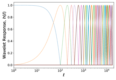
Figure 2: Needlets allow signals to be localized in both real and harmonic spaces. Here we plot the spectral bands used to define our needlets. Wide harmonic-space bands provide better spatial localization, whilst narrow harmonic-space bands enable better separation of signals with different scale, $\ell$, dependence. We balance these two aspects by tuning the width of the bands based on the expected properties of the sky signals. The colors are to aid differentiating one kernel from another. The dotted lines indicate scales that only include Planck data.

III.3 Component Separation

Once in the needlet frame we apply the internal linear combination component separation method. In this section we briefly overview the ILC method and then describe the details of our implementation including: how we estimate the empirical covariance matrix, how we mitigate ILC bias, and how we account for the frequency dependence of the beams.

III.3.1 Internal Linear Combination Method

The ILC method is a highly versatile component separation method that has been applied to a wide range of data sets (Tegmark and Efstathiou, 1996; Tegmark et al., 2003; Bennett et al., 2003; Delabrouille et al., 2009; Planck Collaboration XXII, 2016; Madhavacheril et al., 2020; Aghanim et al., 2019). The method works by modeling the data observed at a set of frequencies, $d_{\nu}(\mathbf{x})$, as

$$d_{\nu}(\mathbf{x})=r^{0}_{\nu}s(\mathbf{x})+n_{\nu}(\mathbf{x}),$$ (4)

where $r^{0}_{\nu}$ is the response function that describes how the signal, $s(\mathbf{x})$, contributes to the sky at frequency $\nu$; and $n_{\nu}(\mathbf{x})$ is the noise term, which contains both instrumental noise and all other sky signals. The label $\mathbf{x}$ is a general label indicating the indexing in the chosen base — thus $\mathbf{x}$ could represent a spatial index for a pixel-space ILC, or the $\ell,m$ index for a harmonic ILC or, as in our case, the needlet frame. The assumptions of the ILC are that the response function is known perfectly, which is generally the case for the signals discussed here, and that the signal is uncorrelated with the noise terms. The ILC solution is a linear combination of the observations to obtain a reconstruction of the signal, i.e.,

$$\hat{s}(\mathbf{x})=\sum_{i}w_{\nu_{i}}(\mathbf{x})d_{\nu_{i}}(\mathbf{x}),$$ (5)

where the weights, $w_{\nu_{i}}(\mathbf{x})$, are obtained by minimizing the reconstructed signal’s variance subject to the condition that the ILC has unit response to the signal of interest, i.e.,

$$\sum_{i}w_{\nu_{i}}r^{0}_{\nu_{i}}=1.$$ (6)

The solution for the weights is given by

$$\mathbf{w}=\frac{\mathcal{C}^{-1}\mathbf{r}^{0}}{\mathbf{r}^{0}\mathcal{C}^{-1}\mathbf{r}^{0}},$$ (7)

where $\mathcal{C}$ is the covariance matrix between observations at the different frequencies and we introduce the vector notation $\mathbf{r}^{0}$ for the vector of responses across frequencies. A detailed description of how the covariance matrix is computed is provided in Section III.3.2.

Whilst this solution minimizes the ‘noise’ on the reconstructed signal, it imposes no constraints on what can contribute to this ‘noise’. In general this ‘noise’ will be composed of instrumental noise and residual contaminant signals. These residual contaminants can potentially bias inferences made with the reconstructed signal and thus it is often of interest to impose additional constraints that force specific contaminants to zero. This technique was developed in Ref. (Chen and Wright, 2009) and Ref. (Remazeilles et al., 2011b) and is known as the constrained ILC. This method decomposes the noise term in Eq. 4 into a set of $N$ contaminants, $c^{i}(\mathbf{x})$, with known responses, $r^{i}_{\nu}$, and a residual noise term, $\tilde{n}$. Thus the observations are given as

$$\mathbf{d}(\mathbf{x})=\mathbf{r}^{0}s(\mathbf{x})+\sum_{i=1,N}\mathbf{r}^{i}c^{i}(\mathbf{x})+\mathbf{\tilde{n}}(\mathbf{x}),$$ (8)

where the different frequencies are represented by the vector notation. A linear combination of the data vector is constructed as before; however, in addition to the constraints of unit response and minimum variance, $N$ additional constraints are imposed such that there is zero response to the contaminants, i.e., $\sum_{i}w_{\nu_{i}}r^{\alpha}_{\nu_{i}}=0$ for $\alpha\in\{1...N\}$. A compact form of the weights in this general case is

$$\mathbf{w}=\mathcal{C}^{-1}\frac{1}{\det{\mathcal{Q}}}\sum\limits_{\alpha}(-1)^{\alpha}\det\mathcal{Q}^{s}_{\alpha}\mathbf{r}^{\alpha},$$ (9)

where

$$\mathcal{Q}_{ij}=\mathbf{r}^{i}_{\nu_{a}}\mathcal{C}^{-1}\mathbf{r}^{j}_{\nu_{b}}$$ (10)

contains the mixing of the different components — note that the zeroth component refers to the signal of interest — and $\mathcal{Q}^{s}_{\alpha}$ is the matrix obtained after removing the $\alpha$th row and the zeroth column. This expression, from Ref. (Kusiak et al., 2023), is a refactoring of the result given in Ref. (Remazeilles and Chluba, 2020).

III.3.2 ILC bias

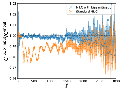
Figure 3: The ILC method requires a frequency-frequency covariance matrix, which is typically not known a priori and therefore must be estimated from the data. This double use of the data, in both the weights and maps in Eq. 5, leads to biases in the ILC map. In simulations, this bias can be seen by computing the cross-correlation of the ILC map with the input component map. The orange line shows the size of this ILC bias in our needlet pipeline when analyzing simulations of a subset of ACT and Planck maps. The shaded contours denote the error on the mean. In this work we introduce a novel mitigation strategy, described in Section III.3.2, and the results of including this in our pipeline are shown in blue. This approach dramatically reduces the ILC bias.

To use the ILC method, an estimate of the frequency-frequency covariance, $\mathcal{C}$, is required. We estimate this locally at every point in each of the needlet frames via

$$\hat{\mathcal{C}}(\mathbf{p})_{ij}=\sum\limits_{\mathbf{p}^{\prime}}T(\mathbf{p}^{\prime})m_{i}(\mathbf{p}+\mathbf{p}^{\prime})m_{j}(\mathbf{p}+\mathbf{p}^{\prime}),$$ (11)

where $T(\mathbf{p})$ is the smoothing kernel. Hereafter we refer to these as “covariance maps”. We choose a smoothed top-hat smoothing function defined as

$$T(|\bm{\theta}|)=\frac{1}{\left(1+\frac{|\bm{\theta}|}{W_{i}}\right)^{6}}.$$ (12)

The width, $W_{i}$, of the top-hat at scale $i$ is set to ensure that we always have a sufficient number of modes so that the covariance matrix is invertible. $W_{i}$ is computed as

$$W_{i}=2\arccos\left(1-2\,\frac{20N^{i}_{\mathrm{elements}}}{N^{i}_{\mathrm{modes}}}\right),$$ (13)

where $N^{i}_{\mathrm{elements}}$ is the number of maps at that needlet scale and $N^{i}_{\mathrm{modes}}$ is the number of harmonic modes selected by the needlet spectral funciton, $h^{(i)}(\ell)$. See the Appendix of Ref. (Delabrouille et al., 2009) for details of this computation. This top-hat smoothing kernel was used as it was found to produce stable measurements of the covariance matrix, especially near the edges of the maps.

When the covariance matrix is estimated from the data, it is well known that a bias can be produced in the component-separated maps (Tegmark et al., 2000; Eriksen et al., 2004; Saha et al., 2008; Delabrouille et al., 2009). This bias, known as the ILC bias, arises due to chance correlations between the noise and the signal. Modes where the signal and noise cancel have lower variance. These modes are up-weighted in the ILC and this leads to a suppression of the signal. We refer the reader to the appendices of Ref. (Delabrouille et al., 2009) for a thorough discussion of this effect. The size of this bias depends on the number of independent modes used to estimate the covariance matrix. When a small number of modes is used, the bias is large. For harmonic ILC analyses, where the empirical covariance matrix is estimated via the standard power spectrum, this bias is only significant for the largest scales since at larger $\ell$ there are more $m$ modes to estimate the power spectrum and so a smaller bias. However, for the needlet ILC presented in this work the problem can affect all scales. To demonstrate this we simulate a subset of the ACT and Planck observations and compare the output ILC to the known input CMB map. For computational speed we simulate a subset of the data: two ACT DR4 maps (at f$150$), two ACT DR6 maps (at f$150$ and f$220$), and three Planck maps (at 100, 143 and 217 GHz); the results should be similar for the full data set. Fig. 3 shows that the resulting map is biased on all scales. This effect arises from one of the strengths of the needlets: the ability to capture spatial variation across the map. In order to maximally account for spatial variation it is best to estimate the needlet covariance matrix on the smallest possible patch of sky, i.e., using a small smoothing kernel in Eq. 11. However, using a small patch of sky means that only a small number of independent modes are used to estimate the covariance matrix. Thus there is a large ILC bias.

In the literature there are a range of approaches to minimize this bias: one could use sufficiently large smoothing scales so the bias is small (Delabrouille et al., 2009), at the possible cost of a loss of the ability to capture spatial variation; the ILC bias could be approximated analytically or computed via simulations and removed (Basak and Delabrouille, 2012); or the ILC method could be modified to minimize a different objective (Remazeilles et al., 2011a; Hurier et al., 2013). In this work we implement a simple alternative method that is motivated by the ILC philosophy of minimal assumptions. Our new approach is to ensure the weights are independent from the data vector by explicitly excluding the data modes, $d_{\nu_{i}}(\mathbf{x})$, from the calculation of the weights at $\mathbf{x}$, $w(\mathbf{x})$, as detailed below. This approach never weights any mode by itself and thereby removes the bias.

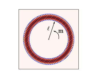
(a) Standard covariance matrix estimation

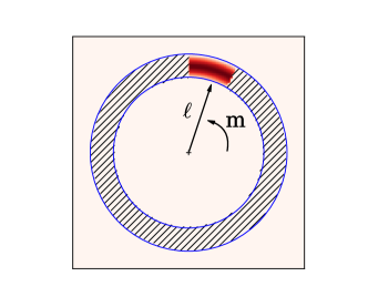
(b) Harmonic-space bias reduction method

Figure 4: A schematic demonstrating the large-scale ILC bias mitigation strategy. The region bound by the blue lines denotes the modes selected at one needlet scale in harmonic space. Radial distance corresponds to $\ell$ and azimuth to $m$. The cross-hatched region shows modes used to estimate the weights and the red region shows the modes to which the weights are applied, hereafter the data vector. In the standard method, (a), the weights are computed from all the modes within the needlet band. The double use of each mode, in the weights and the data vector, leads to the ILC bias. In our mitigation method, (b), the weights are computed from the majority of modes within the needlet band, but we explicitly exclude the data vector modes.

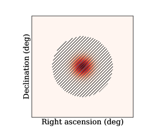
(a) Standard covariance matrix estimation

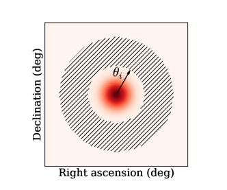
(b) Real-space bias reduction method

Figure 5: A schematic demonstrating the small-scale ILC bias mitigation strategy. These plots show the modes selected at one needlet scale in real space. As in Fig. 4, the cross-hatched region shows modes used to estimate the weights and the red region shows the modes to which the weights are applied, that is the data vector. The double use of modes in the standard ILC, (a), for the weights and the data vector, again leads to the ILC bias. In our mitigation strategy, (b), we simply exclude modes within $\theta_{i}$, the localization scale of the needlet, from the weights.

We trivially demonstrate this for the harmonic ILC method. As is detailed in Appendix B, in the harmonic ILC the weights are applied to the $a_{\ell m}$ modes. The covariance used to compute the weights is the empirical power spectrum. In this case, we can estimate the power spectra using all the $m$ modes except the specific $m$-mode we are trying to reconstruct. This simple modification mitigates the ILC bias. We develop an analogous approach for the needlet ILC; however, isolating subsets of modes is more expensive in the needlet frame. To ensure the method is computationally feasible we use a slightly different approach for the large and small scales – large scales here correspond to $\ell\lesssim 500$. The approach for the large scales exploits the needlet localization in harmonic space, whilst the small scales exploits the localization in real space.

Large-scale strategy: This is very similar to the harmonic ILC case. We can remove a small subset of $a_{\ell m}$ modes from the needlet map. The remaining modes can be used to compute a ‘covariance map’, via Eq. 11, and a set of ILC weights. These weights are then applied to the small number of modes held out. As the weights are now uncorrelated with the data, the ILC bias will be removed. This procedure can be repeated on other subsets until weights have been constructed for all the modes. We refer to this as the ‘harmonic-space bias reduction method’. A schematic of this is shown in Fig. 4. In the needlet frame, this procedure requires four SHTs for each subset considered. As the majority of modes are used in the ‘covariance map’ calculation, we do not need to enlarge the smoothing kernel in Eq. 11. In Appendix C we provide further details of how the subsets are created.

Small-scale strategy: The computational cost of SHTs on small scales motivates us to consider an alternative method for these scales. For these scales we use that fact that the needlets at scale $i$ are spatially localized within some region, $\theta_{i}$, to construct uncorrelated weights. We use a ‘donut’-like smoothing kernel to estimate the ‘covariance maps’, given in Eq. 11. The hole of the donut is set so that the weights will have minimal contribution from the region within $\theta_{i}$ but, through the ring around it, still capture the local map properties. This trivial change to the method can be implemented in a computationally efficient manner — the smoothing is performed with one pair of SHTs. However, it requires slightly larger smoothing scales to ensure there are still enough modes for a stable estimation of the covariance matrix. On the smallest scales we can afford to have slightly larger smoothing scales as the signals tend to vary over scales larger than our smoothing scales. Note we do not use this approach on large scales as we do not want to enlarge the smoothing kernel. We refer to this as the ‘real-space bias reduction method’ and a schematic of this approach is shown in Fig. 5.

In Fig. 3 we show the result of implementing these two methods in our needlet ILC pipeline. These methods reduce the ILC bias by an order of magnitude. The ILC bias is not perfectly removed as neither method produces completely uncorrelated weights: couplings between $m$-modes, induced by effects such as masking, mean that weights from the harmonic-space method are not completely independent from the data modes. For the real-space method, the small overlap between modes in the ‘donut’ and the data modes leads to slight correlations between the weights and data.

When computing the covariance matrix we use one further simplification to reduce the computational cost. We use coadded covariance maps to compute the off-diagonal covariance matrix elements. In our data set we have many measurements of the same patch of sky, with approximately similar noise levels but from different detectors. For example we have five maps of the ‘D56’ region in the f150 band. For each such group of maps, we compute an inverse noise variance weighted coadd and use this map for the off-diagonal covariance matrix. This saves computational time because instead of computing the covariance between each map in the group with every other map in the data set, we just need to compute the covariance between the coadded map and the other maps. This assumes that each map within the group has a similar correlation with the remainder of the data set, which is generally very accurate. Note that this does not lead to biases in the ILC map as generally a misestimation of the ILC covariance matrix leads to suboptimal but unbiased ILC maps. Compared to simply using this coadded map as the input to the ILC, this approach has the advantage that we can easily account for differences in the passbands, gains, and frequency-dependent beams of the observations.

III.3.3 Frequency Response Functions

In addition to the covariance matrix, the ILC method requires a response function that characterizes the strength of each of the components of interest at the frequency of each map. The maps used in this work are all converted to “linearized differential thermodynamic units,” i.e., those in which the response to the primary CMB anisotropies is unity. Thus the frequency response function for the CMB and kSZ effect, in Eq. 7, is simply

$$r^{\mathrm{CMB}}_{\nu}=1.$$ (14)

For all other sky signals the response function requires integrating the spectral function, $f_{\mathrm{X}}(\nu)$, against the instrument passbands, $\tau(\nu)$, as

$$r^{\mathrm{X}}_{\nu,\ell}=\frac{\int\mathrm{d}\nu f_{\mathrm{X}}(\nu)\left.\frac{\mathrm{d}B(\nu,T)}{\mathrm{d}T}\right|_{T=T_{\mathrm{CMB}}}\nu^{-2}\tau(\nu)}{\int\mathrm{d}\nu\left.\frac{\mathrm{d}B(\nu,T)}{\mathrm{d}T}\right|_{T=T_{\mathrm{CMB}}}\nu^{-2}\tau(\nu)},$$ (15)

where the derivative of the blackbody ${\mathrm{d}B(\nu,T)}/{\mathrm{d}T}$ is the conversion to the “linearized differential thermodynamic units”. The $\nu^{-2}$ factors are there by convention: we assume the passband $\tau(\nu)$ quantifies the response to a Rayleigh-Jeans ($\nu^{2}$) source.

In general, the spectral function for the tSZ effect depends weakly on the temperature of the electrons, $T_{e}$, that scatter the CMB photons (Challinor and Lasenby, 1998; Itoh et al., 1998). Given that the temperature of electrons varies throughout the universe, no single temperature value will capture all of the tSZ signal. In this work we consider two approaches: 1) to neglect the temperature-dependent terms, as done in most previous component separation analyses, and 2) to use the scale-dependent temperature proposed in Ref. (Remazeilles et al., 2019). The assumption that the temperature dependence can be ignored is commonly used in the literature (see e.g. Planck Collaboration IV, 2020; Madhavacheril et al., 2020; Bleem et al., 2022), captures most of the signal, and has a simple analytic form. The second case provides a more accurate extraction of the tSZ anisotropies, at the cost of a more complex analysis.

The temperature-dependent terms are important when the electrons are relativistic, i.e., $k_{B}T_{e}\sim m_{e}c^{2}$. The assumption that we can ignore these terms is justified as most electrons in the universe are non-relativistic, i.e., have temperatures $T_{e}\ll m_{e}c^{2}/k_{B}$ where $m_{e}$ is the electron mass, $c$ is the speed of light, and $k_{B}$ is Boltzmann’s constant. In the non-relativistic regime, the tSZ frequency response function is independent of the electron temperature and has the following analytic form:

$$f_{\mathrm{tSZ}}(\nu)=\frac{h\nu}{k_{B}T_{\mathrm{CMB}}}\frac{\exp\left[\frac{h\nu}{k_{B}T_{\mathrm{CMB}}}\right]+1}{\exp\left[\frac{h\nu}{k_{B}T_{\mathrm{CMB}}}\right]-1}-4,$$ (16)

where $h$ is Planck’s constant and $T_{\mathrm{CMB}}=2.726\,$K is the temperature of the CMB (Fixsen et al., 1997; Fixsen, 2009). In keeping with past work, this is our baseline choice for the tSZ spectrum.

For the second approach, we use szpack (Chluba et al., 2012, 2013) to compute the full tSZ frequency response, $g(\nu,T_{e})$. We refer to the response in Eq. 16 as the non-relativistic response and to the response incorporating temperature dependence as the relativistic tSZ response. In Fig. 6 we compare the non-relativistic frequency function to the relativistic one at $T_{e}=8$ keV. Whilst the differences are generally small, they can be important at the precision obtainable with current data.

Following Ref. (Remazeilles et al., 2019), we use a different temperature for each $\ell$, denoted as $\bar{T}_{e}(\ell)$. The scale-dependent temperature accounts for the fact that the largest scale tSZ anisotropies come from the most massive and hottest objects, whilst smaller scale anisotropies come from less massive and cooler objects. The temperature is computed as a Compton-$y$ weighted expectation of galaxy cluster temperatures and we refer the reader to Ref. (Remazeilles et al., 2019) for more details. The relativistic tSZ response is then

$$f^{\mathrm{tSZ-relativistic}}(\nu,\ell)=g(\nu,\bar{T}_{e}(\ell)).$$ (17)

The expected temperatures range from $\sim 8\,$keV on large angular scales to $\sim 2\,$keV on small scales. We discuss the implications of this more extensively in Section V.2.

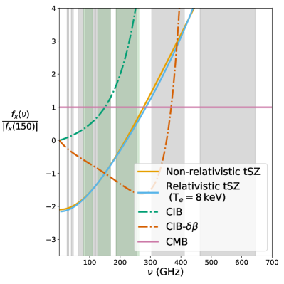
Figure 6: The frequency dependence of the sky signals considered in this work, normalized by the magnitude of the response at 150 GHz. The CMB is shown in pink. The tSZ frequency response depends upon the temperature of the electrons, $T_{e}$, that scatter the CMB photons. Here we compare two cases: first when the temperature is sufficiently low that the electrons are non-relativistic, (gold), and second when the temperature is $T_{e}=8$ keV (blue). In addition to producing a minimum-variance map of the signal of interest, it is often necessary to ensure this map is not contaminated with other sky signals, especially the CIB. To do this we explicitly remove the CIB using the response shown in dot-dashed green. To account for differences between the model CIB spectral energy distribution (SED) and the true SED, we remove sky signals consistent with a second SED, denoted CIB$-\delta\beta$. This second template is obtained from a Taylor expansion of the model SED around the fiducial spectral index, $\beta$. In gray and light green we show a measure of the Planck and ACT passbands respectively. Note that the responses are in “linearized differential thermodynamic” units, hence the unit response of the CMB at all frequencies.

One of the main contaminants for tSZ studies is the cosmic infrared background (CIB). We model the CIB frequency function as a modified blackbody,

$$f_{\mathrm{CIB}}(\nu)=\frac{A\left(\frac{\nu}{\nu_{0}}\right)^{3+\beta}}{\exp\frac{h\nu}{k_{B}T_{\mathrm{CIB}}}-1}\left(\left.\frac{\mathrm{d}B(\nu,T)}{\mathrm{d}T}\right|_{T=T_{\mathrm{CMB}}}\right)^{-1},$$ (18)

where $\beta=1.7$ and $T_{\mathrm{CIB}}=10.70$ K are the parameters characterizing the approximate all-sky CIB modified blackbody SED, $\nu_{0}$ is an arbitrary normalization frequency and $A$ is a normalization constant. These are obtained to fits of a theoretically-calculated CIB monopole at 217, 353, 545 GHz, as calculated in (Planck Collaboration XXX, 2014) using a halo model fit to observations of the CIB anisotropies (McCarthy and Hill, In prep.).

Completely removing the CIB is challenging for two reasons: first, the spectral function is not well known; the functional form used above is a theoretically motivated empirical fit. Deprojecting an inaccurate template leaves residual CIB. Second, the CIB anisotropies exhibit decorrelation across frequencies — i.e., the anisotropies at one frequency are not perfectly correlated with those at a second (Planck Collaboration XXX, 2014; Lenz et al., 2019). This behavior can be understood with a toy model: consider a case where the rest frame SED for the CIB galaxies is the same for all sources. The observed emission is then given by the sum of the redshifted emission from sources over a wide redshift range. This redshifting means that the observed emission at a single frequency comes from many different source frequencies, or equivalently the observed SED of each galaxy is different. Galaxies at different redshifts will then provide a different relative contribution at different observational frequencies. As different frequencies probe different redshift weightings of the sources, the spatial anisotropies will not be perfectly correlated.

For many applications having a small level of residual CIB will not produce any biases; however, for some applications this can be critical. To mitigate the residual CIB we use the method of Ref. (Chluba et al., 2017), hereafter referred to as the moment expansion method — we deproject a second spectral template that represents a Taylor expansion about the assumed CIB spectral index, $\beta$. This model was shown to better account for SEDs that are a sum of modified blackbody spectra, and consequently is a better approximation of the CIB (Chluba et al., 2017). For such studies we provide maps that additionally deproject the derivative spectrum given by

$$f_{\mathrm{CIB-\delta\beta}}(\nu)=\frac{A\ln(\nu/\nu_{0})\left(\frac{\nu}{\nu_{0}}\right)^{3+\beta}}{\exp\frac{h\nu}{k_{B}T_{\mathrm{CIB}}}-1}\left(\left.\frac{\mathrm{d}B(\nu,T)}{\mathrm{d}T}\right|_{T=T_{\mathrm{CMB}}}\right)^{-1}.$$ (19)

Note that each additional deprojection comes at an additional noise cost in the final ILC map, as the additional constraints lead to a less-minimal-variance solution.

To compute the responses with Eq.15, we need the instrument passbands. For ACT we use the Fourier transform spectrometer measurements reported in Ref. (Thornton et al., 2016) for the DR4 data and an upcoming paper for the equivalent DR6 data. For the Planck passbands we use those from Zonca et al. (2009); Planck Collaboration II (2014); Planck Collaboration IX (2014), and we additionally include central frequency shifts as reported in Ref. (Planck Collaboration X, 2016) and Ref. (Planck Collaboration Int. LVII, 2020).

As is discussed in Appendix A of Ref. (Madhavacheril et al., 2020), the finite width of the passbands means that there is a different effective beam for each of the components on the sky. This arises from the combination of two effects: first, each sky signal has a different frequency dependence and thus is more important in different parts of the instrumental passbands. Second, the beam is different at different frequencies (for diffraction-limited optics we have FWHM $\propto 1/\nu$). In this work we follow the method of Ref. (Madhavacheril et al., 2020) and account for this using scale dependent “color corrections”. Scale-dependent color corrections are changes to the frequency response functions that account for the different effective beam seen by each signal. At large scales this effect is negligible; however, the color corrections can be $\gtrsim 10\%$ changes on small scales.

First we compute the scale-dependent responses as

$$r^{X}_{\nu,\ell}=\frac{\int\mathrm{d}{\nu}b(\ell,\nu)f^{X}(\nu)\left.\frac{\mathrm{d}B(\nu,T)}{\mathrm{d}T}\right|_{T=T_{\mathrm{CMB}}}\nu^{-2}\tau(\nu)}{b(\ell,\nu_{0})\int\mathrm{d}{\nu}\left.\frac{\mathrm{d}B(\nu,T)}{\mathrm{d}T}\right|_{T=T_{\mathrm{CMB}}}\nu^{-2}\tau(\nu)},$$ (20)

where $b(\ell,\nu)$ is the frequency dependent beam and $\nu_{0}$ is the reference frequency. The details of the computation of the frequency-dependent beams will be provided in an upcoming ACT paper. Then we compute the weighted average of this across the needlet band to get each component’s response in that band as

$$r^{(i),X}_{\nu}=\frac{\sum\limits_{\ell}r^{X}_{\nu,\ell}h^{(i)}_{\ell}}{\sum\limits_{\ell}h^{(i)}_{\ell}}.$$ (21)

Again following Ref. (Madhavacheril et al., 2020) we do not apply scale-dependent corrections to the lower resolution Planck data as the investigations in Ref. (Planck Collaboration II, 2014; Planck Collaboration IX, 2014) found no evidence for scale-dependent color corrections.

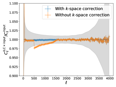
Figure 7: The ACT data are filtered to remove a set of bright contaminants, such as scan-synchronous pickup — see Section III.5 for more details. The orange points show the ratio of the cross-correlation of the ILC map, including the final filter, and input component map to the input map auto-power spectrum. This demonstrates that a non trivial set of modes are impacted by the Fourier-space filter. Using the correction method described in Section III.5 we can correct for these missing modes, with the result shown in blue. With the correction there are no significant biases induced by the NILC pipeline. For reference the gray band shows the $1\sigma$ error on the ILC output power spectrum. The blue and orange error bars are the error on the mean. These errors are very small on large scales as the sample variance cancels in the ratio. For this analysis we use Gaussian simulations of the complete ACT & Planck data set. The largest scales, $\ell\lesssim 500$, only use Planck data, which does not need Fourier-space filtering. The Fourier-space correction thus only impacts larger $\ell$, hence the feature seen at $\ell\approx 500$.

III.4 Inverse Needlet Decomposition

The ILC method produces a set of component-separated maps at each needlet scale, $\hat{s}^{(i)}(\mathbf{p})$. We then need to recombine the maps into a single real-space map, $\hat{s}(\mathbf{n})$. One of the key features of needlets is that this operation is straightforward: one simply convolves each needlet map with the needlet kernel associated with that scale and sums all the resulting maps, i.e.,

$$\hat{s}(\mathbf{n})=\sum\limits_{\ell m}Y_{\ell m}(\mathbf{n})\sum\limits_{i}h^{(i)}_{\ell}\sum\limits_{\mathbf{p}}w(\mathbf{p})Y^{*}_{\ell m}(\mathbf{p})\hat{s}^{(i)}(\mathbf{p}).$$ (22)

Note that for this operation to not lose any information over the scales of interest we require that the needlet spectral functions satisfy

$$\sum_{i}\left(h^{(i)}_{\ell}\right)^{2}=1.$$ (23)

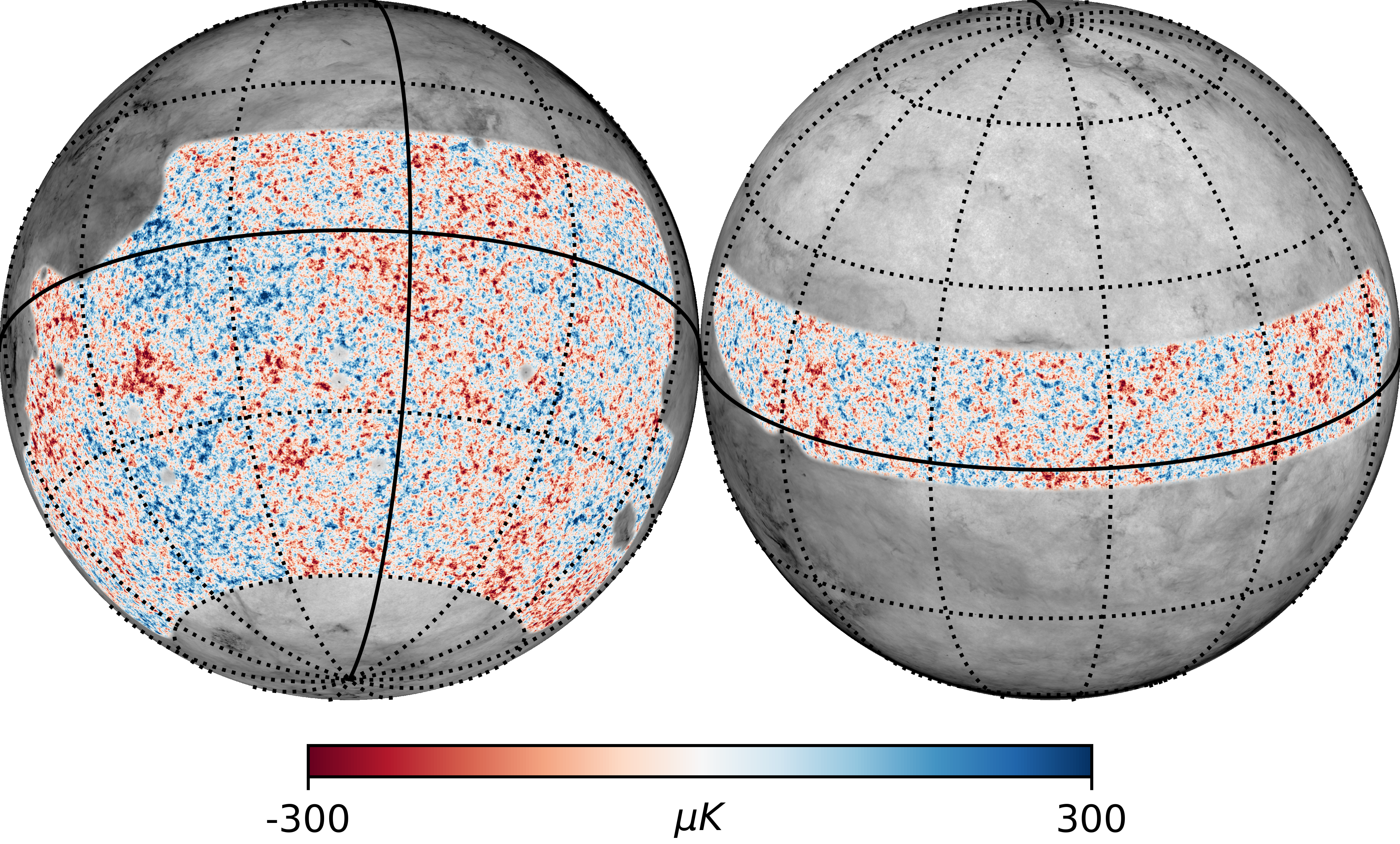
(a) ACT & Planck NILC CMB temperature and kinetic Sunyaev-Zel’dovich anisotropy map.

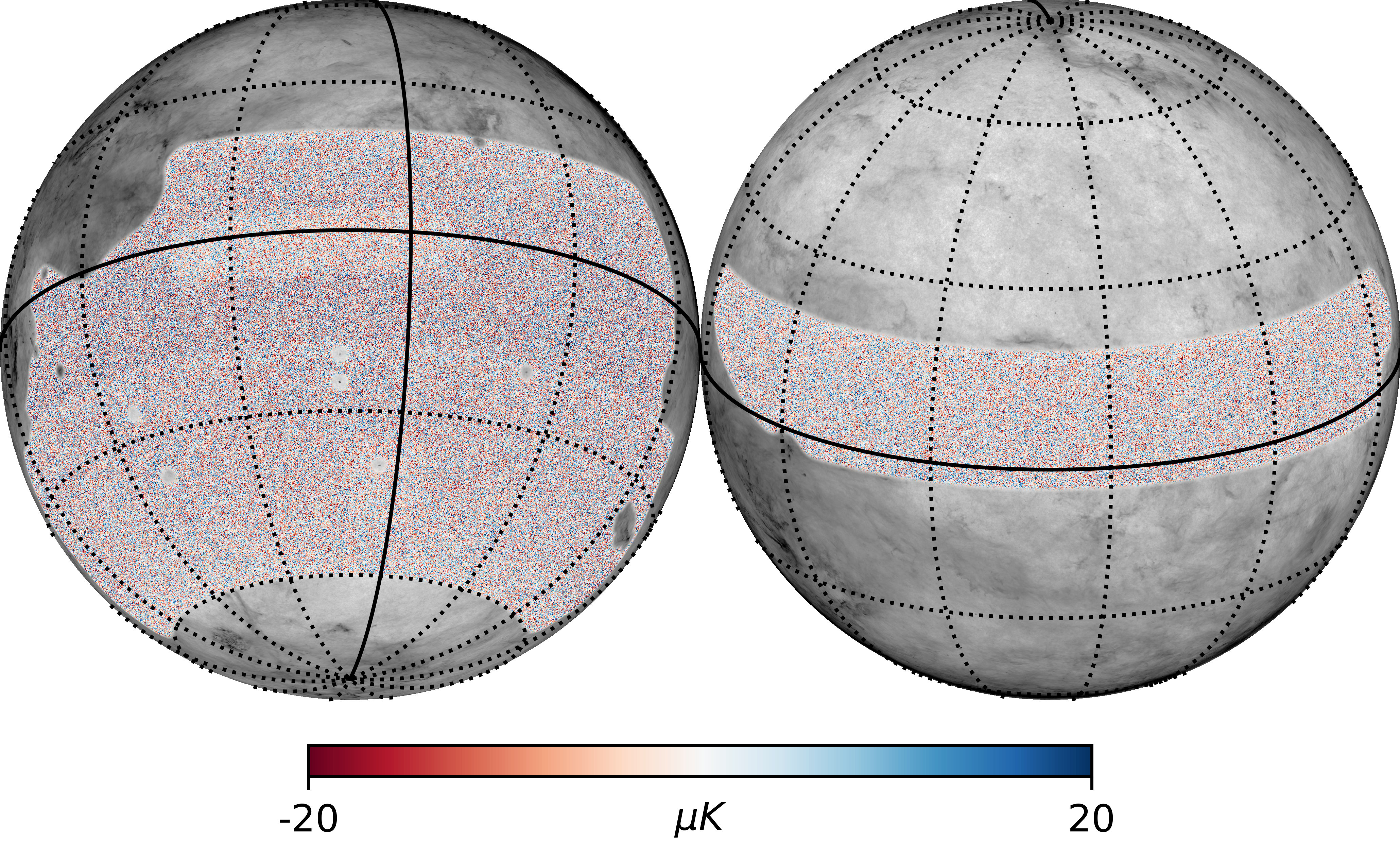
(b) ACT & Planck NILC CMB E-mode anisotropy map.

Figure 8: Maps of two sky components across the full footprint used in this work. Within each of the CMB temperature (a) and CMB E-mode (b) anisotropy maps we can see large-scale CMB fluctuations. The variations in the ACT depth are visible as changes in the small scale noise in the E-mode map. Note that to aid visualization the color scale saturates. The gray scale image in the background is Planck Commander dust map. Bright dusty star forming galaxies and clumps of galactic dust can be seen in many of the holes of the mask, see Fig. 1.

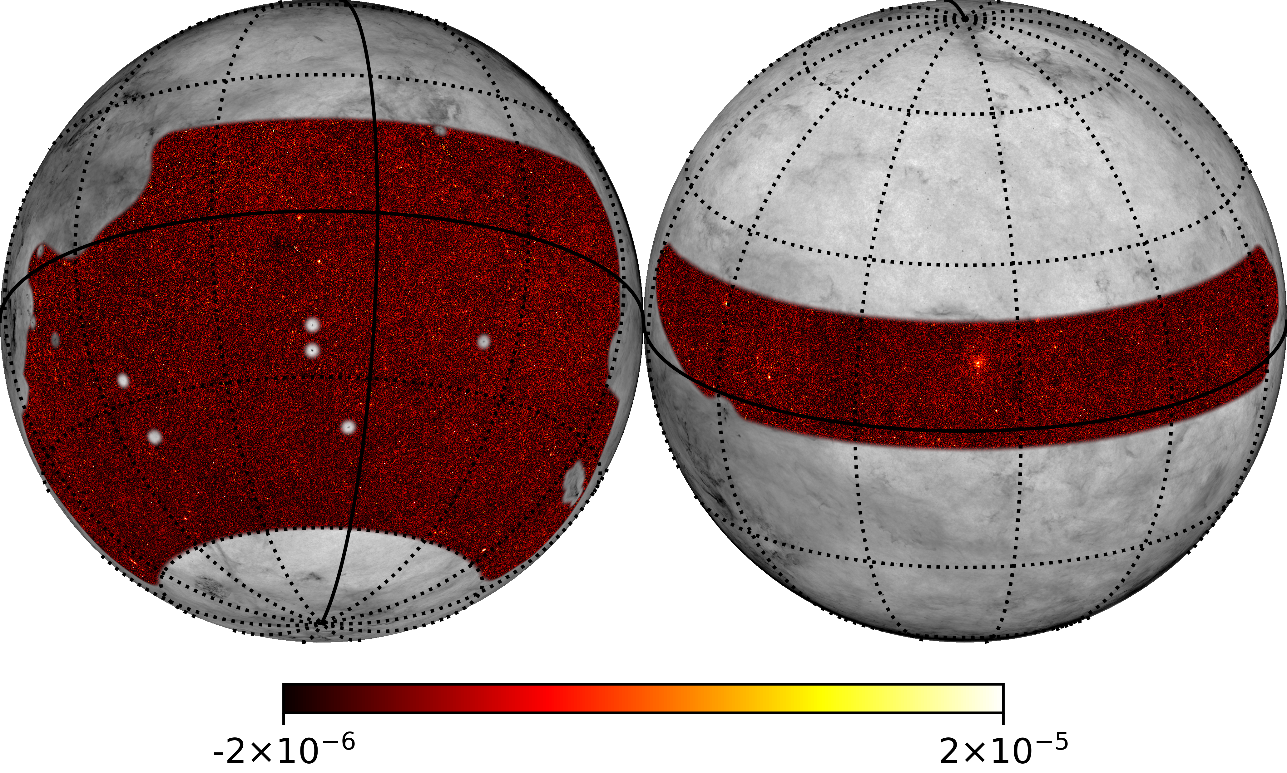
(a) ACT & Planck NILC Compton-$y$ map.

Figure 9: A map of Compton-$y$ across the full footprint used in this work. We can clearly see many galaxy clusters. As in Fig. 8, to aid visualization the color scale saturates and the gray scale background image is the Planck Commander dust map.

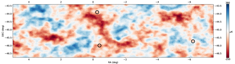
(a) CMB temperature and kinetic Sunyaev-Zel’dovich anisotropy map.

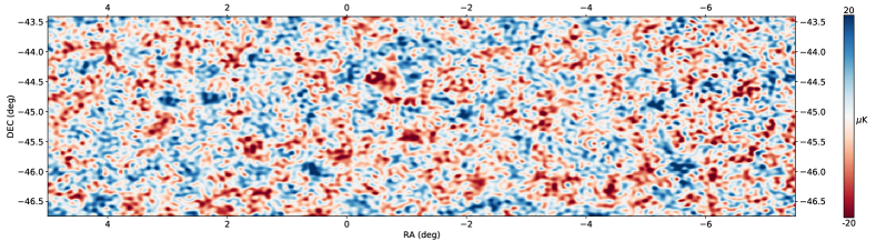
(b) CMB E-mode polarization map.

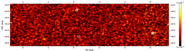
(c) Compton-$y$ map.

Figure 10: A $\sim 30$ deg² region of the component-separated maps for the CMB temperature, CMB E-mode polarization and Compton-$y$ anisotropies. In (a) and (b) the CMB temperature and E-mode anisotropies are clearly visible across a broad range of scales, whilst in (c) we can see numerous bright clusters picked out by the thermal Sunyaev-Zel’dovich effect. A comparison between the CMB temperature and Compton-$y$ maps shows that the separation of the two signals is not perfect — small imprints of tSZ clusters can be seen in the CMB temperature map and we highlight three examples with black circles and their corresponding clusters in the Compton-$y$ map. The increase in noise seen at the right edge of the Compton-$y$ map occurs due to changes in the depth of the ACT maps. Note that the maps appear slightly horizontally stretched as the CAR projection is conformal only at the equator.

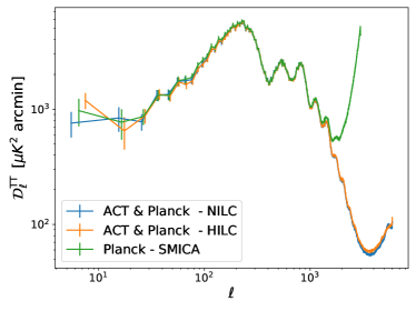
(a) CMB Temperature Anisotropies

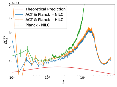
(b) Compton-$y$

Figure 11: The power spectrum of the CMB Temperature and Compton-$y$ NILC maps computed with namaster. We compare these with the corresponding Planck smica CMB and NILC Compton-$y$ maps, and harmonic ILC (HILC) maps produced from the ACT and Planck data. The large increase in power at high $\ell$ (small scales) in the Planck-only data is due to noise in the Planck IlC maps, and is significantly reduced in the ACT & Planck ILC maps. The theoretical prediction for the Compton-$y$ power spectrum was computed with class-sz (Bolliet et al., 2022). The Compton-$y$ map is noise dominated at all scales, hence all the data points lie above the theoretical prediction. The vertical bars denote the errors and are computed analytically via the Gaussian approximation. To aid comparisons we have horizontally offset the points in the plot.

III.5 Fourier-space Filtering Correction

The Fourier-space filtering performed on the ACT maps corresponds to a highly complex operation in harmonic space. This is especially true once the maps have been combined in the needlet domain with satellite data, for which this filtering is not performed. In the ILC, the filtered modes in the satellite data are treated as ‘noise’, due to their absence in the ACT maps, and so are partially removed. For applications that are driven by the smallest scales, such as cluster stacking investigations, the effect of this filtering is minimal as the filter only removes large scale modes. Thus, for studies on these scales the filtering can likely be safely ignored. However, for applications that require modes with $\ell\lesssim 1500$ this effect is non-trivial and extends beyond the power spectrum in a complex and anisotropic manner.

To avoid having to model this complex, anisotropic effect in future analyses we attempt to correct for it at the map level. This is done by infilling the filtered modes using the Planck observations. Specifically, we generate two versions of the component-separated maps: one that uses the complete data set (map A) and another that only uses Planck data (map B). We then filter map A with a filter with the same form as the initial filtering, Eq. III.1.2, but with the filtering parameters increased ($k_{x}$ is doubled whilst $k_{y}^{\mathrm{central}}$ is increased to 1450). We then apply the inverse of the Fourier space filter to map B to isolate the removed modes. Finally we add these isolated modes to the filtered version of map A to obtain a corrected map. The purpose of refiltering with an enlarged filter size is twofold: 1) to ensure we better remove residual scan-synchronous pickup; and 2) to provide a well defined set of filtered modes. The ILC does not remove all the filtered modes from the Planck data set so the output, uncorrected maps have a complicated effective filtering. Applying the larger filter simplifies the effective filter. Even without the correction described here, such a filter would likely still be needed to ensure that the effective filter is well characterized. In Fig. 7 we see that this procedure corrects the leading order effect of the Fourier space filtering. Note that the Fourier-space filter only effects modes with $\ell\gtrsim 450$ as below this only Planck data is used, for which Fourier-space filtering is not needed. This method has a cost: the modes added back into the map typically have larger noise than the other modes. This is because they are obtained from Planck maps that have lower resolution and higher noise. Whilst these maps thus have anisotropic noise, this is a small effect and can be ignored for most applications. We again note that the filtering used in this work is less aggressive than that used in other ACT analyses, e.g., Refs. (Choi et al., 2020) and (Qu et al., 2023), and thus the maps will contain some residual scan-synchronous pickup. For cross-correlations this is unimportant, however for analyses using only these maps, such as CMB-lensing reconstruction or primordial non-Gaussianity searches, tests should be performed to see whether this residual impacts the results. If needed, the output ILC maps can be filtered again to remove any residual contamination, with the cost of also removing some signal modes.

Fig. 7 demonstrates that with our $k$-space correction and ILC bias reduction methods our NILC pipeline produces unbiased maps.

IV Component-Separated Maps

Using this pipeline we produce the key results of this work: component-separated CMB temperature and E-mode polarization anisotropies and Compton-$y$ maps with a maximum scale of $\ell=17000$ ($\sim 0.6$ arcmin). The full-area maps are shown in Fig. 8 and Fig. 9.

In Fig. 10 we show a cut out of the maps of CMB temperature, E-mode and Compton-$y$ anisotropies. There are several interesting features: first, through combining the Planck and ACT measurements, we obtain a CMB temperature map that is dominated by CMB modes, rather than instrumental and atmospheric noise, over a wide range of scales. Without Planck we would not be able to resolve the largest-scale modes and without ACT we would have limited small-scale sensitivity. Secondly, whilst the power spectrum of the Compton-$y$ map is noise-dominated on almost all scales (as discussed in Section V.2), we can clearly see many bright compact objects. These objects are galaxy clusters as the Compton-$y$ anisotropies map out the integrated electron pressure,

$$y(\mathbf{n})=\frac{\sigma_{T}}{m_{e}c^{2}}\int\limits_{los}\mathrm{d}l\,P_{e}(\mathbf{n},l),$$ (24)

where $\sigma_{T}$ is the Thomson cross section, $m_{e}$ is the electron mass, $c$ is the speed of light, and $P_{e}$ is the thermal electron pressure. They are visible above the noise due to the highly non-Gaussian structure of the Compton-$y$ signal. The number of these visible by eye is significantly more than can be seen in the individual frequency maps. Thirdly, by comparing the CMB temperature map and the Compton-$y$ map we can see that the separation of the components is not perfect — the imprint of the brightest SZ clusters can still be seen in the CMB temperature map. As was discussed in Section III.3.1, this arises as the standard ILC method minimizes the total ‘noise’ and not the contribution of any individual foreground sky components. For some analyses this residual extragalactic contamination can be problematic. To alleviate this, we provide CMB temperature maps that are explicitly constructed to have no contribution from the tSZ signal. This comes at the cost of slightly higher noise. These maps are further discussed in Section V.1.

The next notable feature can be seen around right ascension (RA) $\sim-5.5^{\circ}$, where the noise to the left of this line is noticeably lower. The region shown in this cut out coincides with the edge of the ACT “D8” field, as is seen in Fig. 1, and the lower noise occurs through the inclusion of this deep observation in the output map. This boundary highlights a benefit of working in the needlet frame – we can simply and almost optimally combine observations with differing depths and footprints. This feature is only visible in the noise-dominated tSZ map and not the signal-dominated CMB. The continuity of the CMB signal across this boundary provides a simple check of our method.

The E-mode map, like the temperature anisotropies, is signal-dominated over a wide range of scales. As expected, the characteristic scale of the visible E-mode pattern is significantly smaller than the $\sim\,$degree scale features in the temperature maps.

The NILC pipeline does not return error estimates on the maps. Simulations are thus a key means of characterizing uncertainties in analyses using these maps. To facilitate this we provide a suite of simulations of these maps. Two types of simulations are provided: first a small suite of non-Gaussian sky simulations – built with PySM and the Stein et al. (2020) and Sehgal et al. (2010) simulations– and second a set of Gaussian sky simulations. The former is useful for validating analysis pipelines and checking for biases, whilst the later is best suited to characterizing uncertainties. A detailed description of these simulations is given in Appendix A.

V Map Properties

During the generation of these maps we investigate a number of their properties that, when combined with the simulation-based pipeline tests discussed in Appendix A, help provide validation of our analysis methods.

V.1 Properties of the CMB maps

In Fig. 11a, we show the power spectrum of the output temperature map, where for comparison we also show the power spectrum of the equivalent Planck smica (Planck Collaboration IV, 2020) and our harmonic ACT & Planck ILC maps. The power spectra are computed using NaMaster (Alonso et al., 2019). We use bin widths of $\delta\ell=10$ with uniform weight and the error bars are computed analytically with the Gaussian approximation (Wandelt et al., 2001; Efstathiou, 2004). Over a broad range of scales, we see statistical agreement between our ACT and Planck map with the Planck smica map. On the largest angular scales, we find strong agreement with the Planck smica results, as expected as the data are very similar. On the smallest scales we see the dramatic improvement gained by using the small scale ACT data – at $\ell\sim 2000$ the noise, seen as an upturn in the power spectra, is an order of magnitude lower. Although difficult to determine from the figure, the noise level in the harmonic ILC (HILC) map is approximately 10% larger on the smallest scales.

As can be seen in Section IV, the CMB temperature maps still have residual tSZ contamination. Following Ref. (Madhavacheril and Hill, 2018), these residuals can be seen more explicitly by stacking the CMB map at the locations of clusters detected with ACT DR5 data (Hilton et al., 2021). Fig. 12a shows the results of this stacking and a large residual of the tSZ signal can be seen. This residual tSZ signal can bias certain analyses (e.g., Osborne et al., 2014; van Engelen et al., 2014). Using the deprojected ILC, as detailed in Section III.3.1, we can create a CMB map with explicitly zero contribution from the tSZ effect. We then perform the same stacking operation and the results are shown in Fig. 12b. Here we see that the residual is almost completely removed by this procedure. We do see a hint of a small residual signal left at the center of the stack that indicates remaining contamination. A possible source of this contamination is the CIB. CIB galaxies are spatially correlated with the tSZ effect and by stacking on the location of tSZ clusters we are also stacking on CIB galaxies. Further, as is discussed in Ref. (Sailer et al., 2021; Abylkairov et al., 2021; Kusiak et al., 2023) and Ref. (Coulton et al., 2022), when deprojecting the tSZ effect there is often an enhancement of the residual CIB contamination. These two effects combined are thought to give rise to the small residual signal.

ACT has undertaken a blinding procedure for several key science products, detailed in an upcoming paper, including a blinding of the E-mode power spectrum. This is to minimize biases in the inferred cosmological parameters from effects such as confirmation bias. As such we have not yet performed a power spectrum comparison of the CMB E-mode map to Planck data. As is visible in the maps in Fig. 10b, we have significant improvements in the E-mode noise. A quantified version of the improvement can be seen in Fig. 18 of Appendix A.2, where we show the E-mode power spectra of simulated ILC maps. The data are expected to show similar improvements, and will be assessed in a future paper.

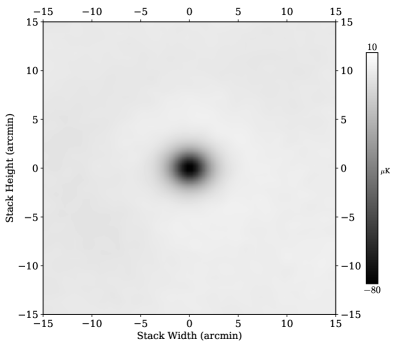
(a) Standard ILC

(b) ILC with tSZ deprojection

Figure 12: Stacks of the CMB temperature anisotropies at the location of tSZ-detected clusters. The stacks are performed on 30 arcmin $\times$ 30 arcmin extracts at the location of clusters in the ACT DR5 cluster catalog (Hilton et al., 2021). If the ILC perfectly removed all the foregrounds from the CMB map we would expect just noise in these stacks. In the base ILC, Fig. 12a, a large signal caused by residual tSZ contamination is visible. This can be mitigated through the use of a constrained ILC, Section III.3.1, as seen in Fig. 12b.

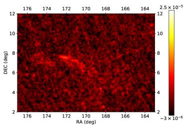
(a) Planck MILCA Compton-$y$ map

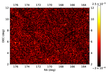
(b) ACT & Planck NILC Compton-$y$ map

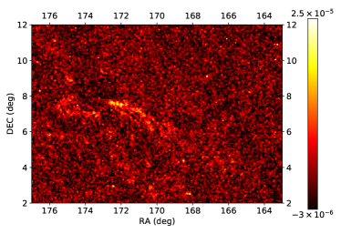
(c) ACT & Planck Harmonic ILC Compton-$y$ map

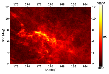
(d) Planck $545$ GHz map

Figure 13: A comparison of the combined ACT and Planck NILC map, the Planck 2015 MILCA map, and a combined Planck & ACT harmonic ILC map of the Compton-$y$ signal on a small $\sim 135$ deg² region of sky. To aid the interpretation of these maps we also show the Planck 545 GHz map in the same patch of sky. The comparison between the Planck MILCA and the ACT & Planck NILC maps demonstrates both the consistency of our results and the benefits of the high-resolution ACT data. The comparison between the harmonic ILC map, the NILC map, and the Planck 545 GHz map shows that working in the needlet frame helps remove the strongly spatially varying Galactic foregrounds. Note that to aid visualization the colorbar saturates.

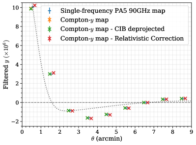
Figure 14: 1D profiles from high-pass filtered stacks of the Compton-$y$ map at the location of tSZ-detected clusters. We perform this stacking operation on four maps: the f$090$ maps from the PA6 detector array, the Compton-$y$ map produced with the non-relativistic tSZ response, the Compton-$y$ map produced with the non-relativistic tSZ response and with the CIB deprojected, and the Compton-$y$ map produced with the relativistic tSZ response. The points with and without the CIB deprojection lie on-top of each other, indicating the measurement is unlikely to be contaminated by CIB emission. Note that the PA5 f$090$ maps has been rescaled into Compton-$y$ units. See Section III.3.3 for a detailed discussion of the relativistic and non-relativistic responses. We apply a high-pass filter to remove correlated noise, as described in Section V.2. To guide the eye, in dashed black we show the scale of the $y$-map beam (1.6 arcmin FWHM) filtered in the same manner as the data. For visualization purposes we have offset the horizontal points.

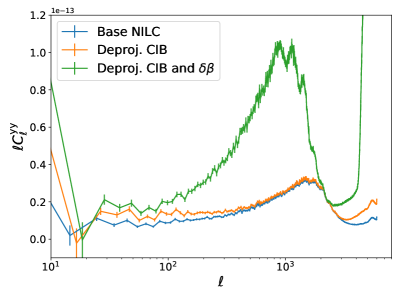
Figure 15: Power spectra of three different versions of the Compton-$y$ ILC map: the base ILC, a map with a fiducial CIB spectrum explicitly removed, and a map where both a fiducial CIB spectrum and a term to account for uncertainties in the CIB SED, labeled by $\delta\beta$ and described by Eq. 19, are removed. Removing these signals provides increasing levels of robustness to contamination but at a cost of increasing noise, seen here as the increase in power on most scales. The power spectra and error bars are computed in the same manner as those in Fig. 11.

V.2 Properties of the Compton-$y$ map

The benefits of the high-resolution data and the needlet basis can be most easily seen by examining the Compton-$y$ map as, unlike the CMB map, the Compton-$y$ map is noise-dominated on all scales. This is demonstrated in Fig. 11b where we plot the power spectrum of the $y$-map and, for comparison, the expected theoretical thermal Sunyaev-Zel’dovich power spectrum from class-sz (Bolliet et al., 2022), the Planck NILC tSZ map power spectrum (Planck Collaboration XXII, 2016), and the harmonic ILC map power spectra. The theoretical model is the same as that used in the Websky simulations (Stein et al., 2020). All the measurements lie above the theoretical expectation due to the noise bias in these autospectra. The ACT and Planck NILC map shows lower noise on all scales compared to the Planck NILC map. On large scales this difference arises as the NPIPE maps have lower noise compared to the Planck-2015 maps used to compute the Planck NILC map. On smaller scales the noticeable improvement comes from the small-scale ACT measurements.

Even at the map level many of these benefits are visible, as is demonstrated in Fig. 13. First, Fig. 13a and Fig. 13b demonstrate the benefits of the high-resolution ACT data – the clusters, visible as bright yellow, point-source-like objects are both better localized and more numerous, demonstrating the depth of the combined $y$-map. Next, it is beneficial to compare the needlet ILC, Fig. 13b, to the harmonic ILC, Fig. 13c. In Section IV we saw that the needlets easily accounted for spatial variations in the map depth, and in the harmonic and needlet ILC comparison we can explicitly see how the needlet frame aids the reduction of spatially varying foregrounds. In the center of the harmonic ILC patch, a bright extended structure is visible, but it is suppressed in the needlet ILC maps. This structure is the imprint of residual Galactic dust, as can be seen in Fig. 13d where we show this region as observed by the dust dominated Planck 545 GHz channel. Through the localization in real-space the needlets are able to treat low dust and high dust regions differently. On the other hand, the harmonic ILC can only operate on the sky-averaged properties.

Examining the profiles of the Compton-$y$ clusters is a powerful test of the Compton-$y$ map. In Fig. 14 we compare the average profile of tSZ clusters as measured in the Compton-$y$ map and in one of the input f$090$ maps, stacked using the ACT DR5 cluster catalog (Hilton et al., 2021). We apply a high-pass filter to remove modes with $\ell<2000$, which are ‘noise’ dominated and contribute correlated noise to the stack. We expect the profiles of the clusters at f$090$ to be similar to the clusters in the Compton-$y$ map, after accounting for the different units and beams. Thus the good agreement seen here demonstrates that our pipeline is not distorting the cluster profiles and amplitudes. Note that, as ACT and Planck are not sensitive to the monopole, the monopole of the Compton-$y$ map is not physically meaningful. Thus the Compton-$y$ map is a map of the fluctuations of the Compton-$y$ field about the mean.

The high sensitivity and large area of these maps means that we need to take particular care to account for potential biases. A key bias in Compton-$y$ maps is the cosmic infrared background (CIB). The dusty star-forming galaxies, which source the CIB, are spatially correlated with the tSZ effect as some of these galaxies occupy the massive halos that source the tSZ effect. Hints of CIB contamination have been seen in previous tSZ analyses (see e.g. Planck Collaboration XXIII, 2016; Schaan et al., 2021; Vavagiakis et al., 2021). As discussed in Section III.3 we can minimize the impact of the CIB by explicitly removing any signal with a specified modified blackbody spectrum and, for cases that are especially sensitive to CIB biases, implementing an additional correction for deviations around this modified blackbody, as described in Section III.3.3. The cost of this additional removal is increased noise that can be seen in Fig. 15, where we compare the power spectra of the base Compton-$y$ map to maps with these different deprojections.

Generally, each additional component deprojected results in a further increase of the noise in the ILC map. This is seen as an increase in power in the power spectrum as the maps are noise-dominated. There are several noteworthy features in the deprojected maps: firstly the noise penalty of the deprojections is highest on scales where only ACT data contributes (the smallest scales). This arises because ACT lacks the very high Planck frequency channels that have strong sensitivity to the CIB. Without these channels it is difficult to separate the tSZ and CIB, hence the large noise increase. The noise starts to increase around $\ell\sim 3000$ as this is where the high frequency Planck data becomes noise-dominated. This increase is more significant when more components are deprojected. Interestingly on the scales with $1400\lesssim\ell\lesssim 2500$, there is no noise penalty for deprojecting just the CIB and, in a smaller range of scales, no cost for deprojecting both the CIB and the correction term. This occurs on scales where the noise in the ILC map is dominated by non-CIB contributions. In this regime, noise in the CIB deprojected ILC maps is not set by the ability to separate the CIB and tSZ components, but instead the noise arising from the other components (in this case atmospheric noise and residual CMB).

As an example of how these maps can be used in an analysis, we highlight the workflow used in an upcoming cross-correlation analysis of ACT and unWISE galaxies (Kusiak et al., In prep.). A component of this analysis is the cross-power spectrum between the ACT & Planck Compton-$y$ map and the unWISE galaxy catalog (Meisner et al., 2017; Krolewski et al., 2020, 2021; Kusiak et al., 2022). The unWISE galaxies are highly correlated with the CIB (Kusiak et al., 2023). To test the sensitivity of this analysis to the CIB, we compare power spectra measurements from the base NILC $y$ map with the CIB-deprojected $y$ map. As can be seen in Fig. 16, where we show the results from (Kusiak et al., In prep.) for the unWISE “blue” subsample (of mean redshift $z=0.6$), deprojecting the CIB leads to a significant shift in the measurement. Further, when different spectral indices $\beta$ are assumed for the deprojected CIB, statistically significant shifts are observed. This suggests that this analysis is strongly sensitive to contamination from CIB such that the CIB SED needs to be carefully modeled. One means of mitigating this is to use the moment expansion method, discussed in Section III.3.3, and deproject the derivative term as well. As can be seen in Fig. 16, the use of the moment expansion leads to results that are more robust to the choice of CIB parameters. The small differences between the true CIB SED and the assumed model are absorbed by the correction term, and all curves with the moment expansion deprojection, the solid lines in Fig. 16, converge around the same values for $\ell\lesssim 2500$. The efficacy of the moment expansion method in accounting for uncertainties in the spectral properties of a contaminant has also been seen in Ref. (Azzoni et al., 2021), where they use the same approach to remove Galactic dust emission. As a second example, consider the stacked profiles shown in Fig. 14. We can minimize any potential bias by performing the stack on a CIB-deprojected map. However, the points are essentially unchanged, as seen in Fig. 14, and this result is stable to variations in the CIB spectral index. This suggests that for that analysis CIB contamination is less severe and there is no need to deproject the CIB or the derivative. The difference in sensitivity arises as these two example analyses are sensitive to halos of very different mass and redshift.

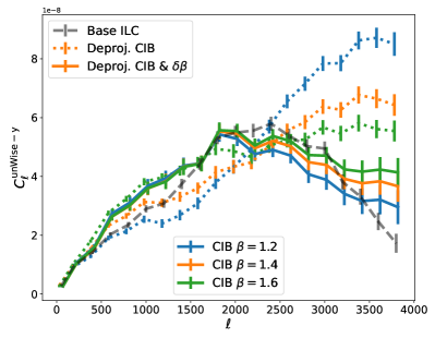
Figure 16: A preview of preliminary results from Ref. (Kusiak et al., In prep.) – an upcoming analysis of correlations between the tSZ effect and the unWISE galaxies. Here we show the cross-correlation of the Compton-$y$ map with the unWISE “blue” subsample, of mean redshift $z=0.6$. The measured Compton-$y$ – unWISE power spectrum shows evidence of CIB contamination, as seen in the difference between the measurement on ILC maps with and without CIB deprojection. Due to the strong physical correlation between the unWISE and CIB galaxies, this analysis is also sensitive to how the CIB is removed and choosing different parameters for the CIB spectral index leads to different results. One method of mitigating this is to also deproject a correction to the CIB SED, given in Eq. 19. This term helps correct for any mismatch between the true SED and the assumed model. As shown by the solid lines, this approach leads to results that are more robust to modelling choices. Note both the unWISE and Compton-$y$ maps are dimensionless.

Finally we compare the results of using the non-relativistic and relativistic tSZ responses. Using the non-relativistic response can bias the resulting $y$-map as is discussed in Ref. (Hurier and Tchernin, 2017; Erler et al., 2018) and Ref. (Remazeilles and Chluba, 2020). The importance of this difference can be most directly seen in the tSZ cluster stacks – in Fig. 14 we compare stacks of detected galaxy clusters in a Compton-$y$ map made using the non-relativistic temperature response, Eq. 16, and the average temperature response, Eq. 17. We see that the profiles in the latter case are $\sim 5\%$ larger, with the difference arising as the standard tSZ map is biased low by the ignored relativistic SZ contributions.

VI Conclusions

Sky Component	Deprojected components	Notes
CMB temperature and kinetic Sunyaev-Zel’dovich	tSZ
	CIB (T${}_{\mathrm{CIB}}=10.7$ K, $\beta=1.7$)	$\ell_{\mathrm{max}}=17000$
	tSZ & CIB
CMB E-mode	None	$\ell_{\mathrm{max}}=4000$
Compton-$y$ relativistic and non-relativistic	CIB
	CIB & CIB correction	$\ell_{\mathrm{max}}=17000$
	CIB & CMB

Table 3: A summary of the maps to be delivered. In addition to the minimum-variance ILC map, we produce CMB temperature and Compton-$y$ maps that deproject one or more components. All maps are convolved to a 1.6 arcmin FWHM Gaussian beam.

We have presented component-separated CMB temperature, CMB E-mode polarization, and Compton-$y$ maps that trace the integrated gas pressure. These maps were produced with a needlet ILC pipeline, designed to take advantage of the different localization of key map properties. To mitigate the well-known “ILC bias” we developed a simple scheme that helps ensure that the resulting ILC maps have no significant loss of the signal.

In addition to the ILC bias, we explored biases arising from residual foreground contamination in the “cleaned” ILC maps. These residuals are left from the imperfect separation of sky signals. The importance of these residuals depends on the analysis in question, but for many analyses these residuals can cause important biases in cosmological and astrophysical inferences. For such analyses we have created a set of constrained ILC maps, as described in Ref. (Remazeilles et al., 2013), that have one or more foregrounds explicitly removed – at the cost of extra noise. The derived products with different deprojections are summarized in Table 3. It is important to note that the Fourier space filtering used in this work removes fewer modes than previous ACT analyses. This means that there may be small scan-synchronous pickup residuals in the maps. For cross-correlation studies this can be safely ignored, but other analyses should perform tests to ensure their results are not impacted by residual scan-synchronous pickup. Further the Fourier space correction introduces a small amount of anisotropic noise.For most analyses this can be ignored, but if it is important then optimal filtering routines (e.g. Wandelt et al., 2004; Smith et al., 2007) that incorporate the anisotropic structure of the noise can be used to maximally utilize these maps.

Finally, there are additional observational systematic effects that can impact this analysis. As discussed in Ref. (Madhavacheril et al., 2020) and Ref. (Dick et al., 2010), atmospheric transmission, calibration errors and passband uncertainties can alter the signal seen at each frequency. The passband and gain uncertainties for ACT result in $\sim 1.5\%$ variations in the amplitude of the tSZ signal in each channel (note that f220 has larger variations, which is partly driven by the null of the tSZ effect at $217\,$GHz and partly by the larger uncertainty). In Appendix D we explore the impact of these systematic effects in detail and find that the uncertainties in the passbands, beams, and calibrations lead to negligible changes to stacked cluster profiles from the Compton-$y$ map. Whilst this result cannot easily be related to the precise impact of these instrumental effects on other scientific analyses, it suggests the size of these effects in the Compton-$y$ map are small.

The NILC maps isolate the component of interest whilst minimizing noise and, particularly when using deprojections, contaminants. This makes these ideal for a broad set of science cases; previous component-separated ACT maps have been used for analyses ranging from detailed studies of individual clusters and filaments (Hincks et al., 2022), to studies of galaxy group and cluster astrophysics with large ensembles (Amodeo et al., 2021; Schaan et al., 2021; Kusiak et al., 2021; Gatti et al., 2022; Lokken et al., 2022), to studies of the distribution of matter with lensing (Darwish et al., 2021). The maps presented here will enable the statistical power of such analyses to be significantly increased – the noise in the Compton-$y$ map presented here is similar to that of the deeper “D56” map from Ref. (Madhavacheril et al., 2020) but over an area of sky that is $\sim 25\times$ larger. Likewise, the large improvement in resolution over the Planck component separated maps, seen in Fig. 11, would be highly beneficial to the many analyses based on these maps (e.g. Hill and Spergel, 2014; Hurier et al., 2015; Planck Collaboration XXIII, 2016; Planck Collaboration Int. LIII, 2018; Planck Collaboration IX, 2020; Carron et al., 2022).

It is important to note that there are classes of analysis for which the individual frequency maps would be more appropriate to use; this includes those that require high-precision characterization of the NILC noise. For example, analyses of the power spectrum of the primary CMB anisotropies are likely best done with the frequency maps as modelling the foregrounds with a parametric model enables explicit marginalization over the foregrounds. Furthermore, that approach facilitates fine-grained modeling of instrumental systematics and noise. Precisely modeling the power spectrum of the NILC noise and propagating the associated uncertainties, which would be necessary to robustly extract the primary CMB contribution from the maps presented here, would be equivalent to modelling the frequency channels separately, with the added complication of propagating these components through the NILC pipeline. Thus, the analysis of the power spectrum of the primary CMB anisotropies for ACT DR6 is expected to be done with the frequency maps. Similarly these maps were not used in the recent ACT DR6 lensing analysis. Whilst component-separated maps have been used in past lensing analyses (Planck Collaboration VIII, 2020; Carron et al., 2022), the challenges in dealing with the complex ACT noise (discussed in Ref. (Atkins et al., 2023; Qu et al., 2023)) motivated a simpler analysis of the individual frequency maps.

Finally, these maps overlap with numerous ongoing surveys, such as the Dark Energy Survey (Dark Energy Survey Collaboration et al., 2016), Hyper Suprime-Cam (Aihara et al., 2018) survey, and Dark Energy Spectroscopic Instrument (DESI Collaboration et al., 2016) survey, and therefore are very well-suited for a range of cross-correlation studies. The pipeline developed in this work is highly versatile and can be used to map other sky signals or be applied to other data sets, including upcoming CMB missions such as the Simons Observatory (Ade et al., 2019) or CMB-S4 (Abazajian et al., 2016).

Appendix A Simulations

Simulations are a key part of many analyses and so we also provide simulated component-separated maps. We provide two main simulation products: simulated non-Gaussian sky maps and Gaussian simulations, using the methods developed in Ref. (Atkins et al., 2023). These two products allow tests of different aspects of analysis pipelines: the non-Gaussian simulations are ideal for studying the properties of fields like the Compton-$y$ maps, where signal non-Gaussianity is highly important, whilst the Gaussian simulations are useful for computing ensemble quantities that require large numbers of simulations.

Specifically, the available products are:

• Four different non-Gaussian realizations of the ACT region of the sky (two from the Websky and two from the Sehgal et al. simulation suites). Each sky realization is provided with instrumental and atmospheric noise simulated via two complementary models - a wavelet model and a tiled model.

• Wavelet and tiled noise models, with associated code, that can be used to generate Gaussian simulations of the ‘ILC’ noise in the blackbody and Compton-$y$ maps.

• A small number of end-to-end Gaussian sims of the blackbody and Compton-$y$ maps – 10 each for the tiled and wavelet models. These are the products of processing Gaussian simulations of the input data sets through the NILC pipeline.

All of these products are produced with $\ell_{\mathrm{max}}=10000$.

A.1 Non-Gaussian Simulations

These simulations are composed of three components: Galactic signals, extragalactic signals, and instrumental and atmospheric noise. We generate a non-Gaussian realization of the Galactic sky signals using PySM; we include free-free, synchrotron, thermal dust and Anomalous Microwave Emission (AME) in temperature and the thermal dust and synchrotron signals in polarization (Thorne et al., 2017; Zonca et al., 2021).

For the extragalactic signals we use two different suites of simulations: the Websky simulations and the Sehgal et al simulations (Li et al., 2022; Stein et al., 2020; Sehgal et al., 2010). These two suites both provide one full-sky realization of the lensed CMB sky, the thermal and kinetic Sunyaev-Zel’dovich effects, the CIB, and radio galaxies. The two suites of simulations assume different physical models for each of the components. We refer the reader to Ref. (Sehgal et al., 2010) and Ref. (Stein et al., 2020) for the detailed differences of the modelling. When compared, these simulations provide some measure of the importance of our modeling uncertainties. Unfortunately each simulation only has a single realization, which can limit some studies. However, as the ACT footprint covers only $\sim 1/3$ of the sky, we can rotate the sky and construct a second simulation of the ACT footprint from these simulations. Specifically, we generate the first realization by cutting out the ACT footprint from the full-sky simulation and generate the second realization by first rotating the simulations by 90^∘ and then cutting out the ACT footprint. Note that this cannot easily be done for the Galaxy due to its spatial anisotropy.

The final component is simulations of the noise. For Planck we use the end-to-end NPIPE noise simulations (Planck Collaboration XII, 2016). For ACT we generate simulations using the models described in Ref. (Atkins et al., 2023); one set using the tiled noise model and a second set using the wavelet noise model. By providing simulations from both of the noise models, it will be possible to test how the uncertainties in our noise modelling impact each analysis.

Bringing these pieces together, for each map in our data set we generate a simulated sky by combining the PySM Galaxy with either the Websky or Sehgal et al. simulations at the same frequency. These maps are then convolved with the appropriate instrument beam. Next we add instrumental noise to this to complete the mock observation. We repeat this operation for each map and then input these maps into the needlet ILC pipeline. Note that in these simulations we use Dirac delta function passbands, i.e., the simulations are evaluated at each single frequency, and the ACT maps here have no simulated transfer function.

As a first use case of these simulations, we compare the stacked profile of tSZ clusters in the input map to those in the output needlet ILC Compton-$y$ map, with the results shown in Fig. 17. We find very good agreement between the two sets of stacked profiles and thereby validate this aspect of our pipeline. A benefit of having simulations is that we can analyze each component of the map separately, exploiting the linearity of the ILC method. Thus, we can explore how just the CIB component contributes to the final tSZ map. These maps are useful for understanding residual signals in the maps and for assessing potential biases.

These simulations have a few key limitations: firstly, we only have four sky realizations, given by the two rotations of the two simulations. Secondly, the sky power of these simulations does not match the data – whilst the Websky and Sehgal et al simulations are sophisticated models of the sky, they do not perfectly capture all the components, leading to differences in the size of each sky component. For example, the small scale power arising from the discrete nature of the CIB and radio galaxies is not accurate. Additionally, there are minor limitations (e.g., delta function passbands and simple beam treatments) that prevent tests of certain systematic effects. Despite these limitations, they are invaluable for analyses of non-Gaussian aspects of the sky.

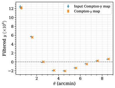
Figure 17: A validation of the Compton-$y$ map with the Websky simulations. We compare the stacked NILC Compton-$y$ map with the true input Compton-$y$ map. The stack is performed on all halos with $M>5\times 10^{14}$ M_⊙/$h$ and these maps are high-pass filtered in the same manner as the data in Fig. 14.

A.2 Gaussian Simulations

To complement the non-Gaussian simulations we provide noise models as described in Ref. (Atkins et al., 2023). These allow the fast generation of many realizations of the noise in the needlet ILC maps and are ideal for investigating ensemble properties of the ILC map’s noise.

We generate these noise models using a two stage process: first, we obtain a model of the sky components present in the input maps. For this purpose we use the Ref. (Dunkley et al., 2013) model, extended to include power laws for the Galactic dust, synchrotron, Anomalous Microwave Emission, and free-free, and a white noise component of arbitrary amplitude and correlation across the maps to account for the Poisson contribution of point sources. The latter component is necessary as we remove all detected sources in each map, rather than those down to a specific flux cut, and this results in each map having a slightly different level of Poisson power. The strength of this correlation across the input maps varies due to the different ratio of radio to dusty sources in each map. Further, we modulate the Galactic dust components by a smoothed version of the Planck dust intensity map. Without this modulation the large scale power in the component separated maps is significantly below that of the data, highlighting how the spatial variations of the Galaxy complicate component separation.

Second, we use this sky model to simulate observations of the sky. We use the same methods as in Appendix A.1 to simulate the instrumental noise and beams. We then process these simulations with the needlet ILC pipeline. From the resulting needlet ILC maps, we subtract the input realization of the signal of interest, e.g., for the CMB ILC maps we subtract the CMB power; this gives a map of the NILC ‘noise’. Using the tools developed in Ref. (Atkins et al., 2023) we then construct tiled and wavelet noise models. These noise models allow arbitary numbers of realizations of the NILC ‘noise’ to be generated. The noise realizations can then be combined with realizations of the signal to provide a simulated map.

The end-to-end Gaussian simulations produced in generating the noise model allow further tests of potential biases in our pipeline. As discussed in Section III.5 and seen in Fig. 3, these simulations can be used to assess the level of bias in our ILC maps. We find no significant biases across the full range of scales. In Fig. 18 we compare the power spectra of simulated Planck-only to Planck & ACT ILC E-mode maps. This demonstrates the value of combining the ACT data with Planck.

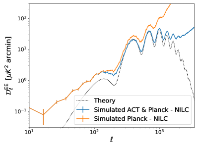
Figure 18: The E-mode auto power spectrum of a simulated Planck-only ILC map and a simulated Planck & ACT ILC map. It can clearly be seen that the ACT data allow the E-modes to be probed to significantly smaller scales.

Appendix B Harmonic ILC

Instead of working in the needlet domain, the ILC method can be applied in the harmonic domain – hereafter the harmonic ILC. In this work we use the harmonic ILC as a baseline to compare against the NILC results, and to build intuition for the bias reduction methods, as the harmonic frame is conceptually simpler. In this Appendix we outline the harmonic ILC method and describe the harmonic-domain implementation of our ILC bias mitigation method.

For the harmonic ILC we have

$$\hat{s}_{\ell m}=\sum\limits_{i}w_{i}a^{i}_{\ell m}$$ (25)

where the weights are defined in Eq. 7. The empirical covariance matrix, $\hat{\mathcal{C}}$, required to compute the weights is simply the estimated power spectra

$$\hat{\mathcal{C}}_{ij}=\frac{1}{N_{\mathrm{modes}}}\sum\limits_{L-\delta\ell<\ell\leq L+\delta\ell}\sum\limits_{m}a^{i}_{\ell m}{a^{j}}^{*}_{\ell m},$$ (26)

where we compute the power spectrum over a range of $\ell$, quantified by 2$\delta\ell$ and $N_{\mathrm{modes}}$ is the number of modes in each bin. We average over a small range of $\ell$ to improve the estimate of the covariance matrix and minimize the ILC bias. To further minimize ILC bias we introduce an ILC bias reduction method, in a similar manner to those discussed in Section III.3.2. When computing the ILC weights for mode $m$ we exclude that $m$ mode from the covariance matrix estimation, Eq. 26. To avoid the computational cost of estimating the covariance matrix $\ell$ times per scale, we instead split the modes into $N=10$ subsets (eg., the first $\ell/N$ $m$ modes are assigned to subset 1 etc) and, for each subset, estimate the covariance matrix with all modes not in that subset. This allows the ILC bias to be mitigated with reduced computational overhead, at the cost of a slight increase in the resulting ILC map’s noise. In fact, whilst the standard method of estimating the covariance matrix has lower noise, it is biased low. When we correct for this bias, by dividing out a transfer function, we tend to find almost identical noise levels to those of our method.

When computing harmonic ILC maps we use the same steps as the needlet ILC pipeline, described in Section III, including the frequency dependent responses.

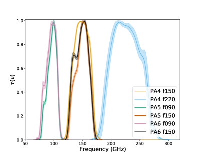
Figure 19: The passbands for the six different ACT DR6 data sets. These are used in Eq. 15 to compute the responses to each sky signal. The shaded region denotes the $1\,\sigma$ uncertainty on these measurements.

Appendix C Mitigating the large scale ILC bias

As described in Section III.3.2, we mitigate the large scale ILC bias by isolating a subset of the modes from the needlet band and using the remainder to compute the ILC weights. In detail this isolation can be performed as follows: starting from the map of anisotropies at a given needlet scale, we perform a SHT. We apply a filter that selects a subset of $a_{\ell m}$ modes and then we perform a second SHT to transform these modes back to the needlet frame; we call this the ‘data map’. This ‘data map’ is then subtracted from the original needlet map. This new map contains all the modes except the held out modes and we use this map to compute the ‘covariance maps’ and ILC weights. The ILC weights are then applied to the ‘data maps’. This procedure is repeated with the next subset of $a_{\ell m}$ modes etc. The resulting ILC maps from the subsets are then added back together to obtain the ILC solution for that needlet scale.

Whilst the approach of removing a subset of $a_{\ell m}$ modes is very similar to the harmonic ILC, described in Appendix B, there is a slight additional subtlety in the needlet frame. When we remove $a_{\ell m}$ modes from the needlet band, the localization of the needlets is altered. If we were to systematically remove each single $a_{\ell m}$ mode the change in the localization of the covariance matrix would be negligible. In practice this would not be effective as effects such as masking and non-Gaussianites mean that each $a_{\ell m}$ mode is not independent. Thus this would only reduce, but not eliminate, the ILC bias. Further, removing modes from the needlet basis requires spherical harmonic transforms, and so this operation comes at a significantly increased computational cost. Hence, this motivates our choice to remove small subsets of $a_{\ell m}$ modes across the band.

The decision of how many subsets to use, $N_{\mathrm{subset}}$, and how to divide the modes into these subsets was made by ensuring the localization of the covariance matrix is not strongly altered. This is balanced by computational time (more subsets is slower) and stability (changing masks and power spectra in simulations should not dramatically change the ILC maps). We use $N_{\mathrm{subset}}=5$. For our footprint the strong correlations from the mask led us to assign $\ell<4$ to subset 1, $4<\ell<8$ to subset 2 etc up to $\ell=20$. Beyond $\ell=20$, the assignment is based on the $m$-mode at each $\ell$. Modes with $0\leq m<\ell/N_{\mathrm{subset}}$ are assigned to subset $\ell/20$ MOD $N_{\mathrm{subset}}$. Modes with $\ell/N_{\mathrm{subset}}\leq m<2\ell/N_{\mathrm{subset}}$ are assigned to subset $1+\ell/20$ MOD $N_{\mathrm{subset}}$ etc. The adjacent $m$-modes are assigned to the same subset as these are most tightly coupled by effects such as masking. Further, by removing different $m$-modes for each $\ell$ we ensure that the localization of the new covariance matrix closely approximates the original covariance matrix. This is additionally aided by our smoothing operation and the fact that we remove only a small subset of the total modes in the needlet band. One might worry that the small set of modes that the covariance matrix is applied to correspond to some highly non-local feature in the maps. However, this is not an issue due to the linearity of the ILC method: in the standard ILC identical results are obtained if the ILC weights are applied mode-by-mode or applied to all modes simultaneously. Instead it is important that the covariance matrix, and hence the weights, remains highly localized and we ensure this with the choices described above.

Appendix D Instrumental Systematic Effects

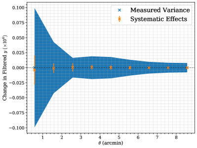
Figure 20: The absolute change in the stacked cluster profiles, Fig. 14, caused by the calibration, beam, and passband uncertainties. These effects, shown in orange, are significantly smaller than the measured scatter in the stack, shown as a blue band.

The key instrumental systematic effects that impact our analyses arise from the miscalibration of the input maps and uncertainties in the passbands and beams. All of these effects can be expressed as changes to the ILC responses, ${r}_{\nu}$ in Section III.3.1, and are important as they control how maps are combined to extract the signal of interest. If these are misestimated the resulting ILC map can be biased. In this section we investigate how significant these biases can be.

The impact of a miscalibrated map is simply a rescaling of the ILC responses $\mathbf{r}_{\nu}\rightarrow(1+\delta c)\mathbf{r}_{\nu}$, where $\delta c$ is the amplitude of the miscalibration. Note that the miscalibration factor is the same for every signal on the sky. On the other hand, the passband misestimation affects each sky component differently. The impact on each of the responses can be assessed by recomputing them with altered passbands, i.e., changing $\tau(\nu)$ in Eq. 20. Beam uncertainty has two impacts: firstly, it acts as a scale dependent miscalibration, given by the ratio of the estimated beam to the true beam. Secondly, it alters the color correction to the response, given in Eq. 20.

To assess the importance of these terms we sample calibration factors, passbands, and beams within their uncertainties. For the Planck passbands we shift the central frequencies based on the uncertainties reported in Ref. (Planck Collaboration Int. LVII, 2020) and use the calibration errors reported in Ref. (Planck Collaboration Int. LVII, 2020). The Planck beam errors have been shown to be negligible (Planck Collaboration V, 2020) and so are neglected here. For ACT DR4 we use the same calibration and beam uncertainties as are included in the power spectrum analyses (Louis et al., 2017b; Choi et al., 2020; Lungu et al., 2022) and use the passband errors from Ref. (Madhavacheril et al., 2020). For DR6 errors we use similar procedures to compute the equivalent errors, with the details of this provided in an upcoming ACT paper. The passbands used in this work, with their errors, are shown in Fig. 19.

In Fig. 20 we show the impact these effects have on the stacked Compton-$y$ profiles. No systematic shift is observed and the spread caused by these effects is negligible.

This result does not ensure that instrumental systematic effects are negligible for other science use cases. In particular the beam uncertainties are scale dependent (and are generally larger on small scales) and the passband uncertainties will likely become more important in analyses that require multiple deprojections. Instead, if instrumental effects are a concern, this analysis should be repeated. Despite these limitations, these results can be used to estimate the size of the effect.

References

- Naess et al. (2021) S. Naess, S. Aiola, N. Battaglia, R. J. Bond, E. Calabrese, S. K. Choi, N. F. Cothard, M. Halpern, J. C. Hill, B. J. Koopman, et al., Astrophys. J. 923, 224 (2021), eprint arXiv:2104.10264.
- Baxter et al. (2018) E. J. Baxter, C. H. Blake, and B. Jain, Astron. J. 156, 243 (2018), eprint arXiv:1808.00415.
- Planck Collaboration Int. XXXIV (2016) Planck Collaboration Int. XXXIV, Astron. Astrophys. 586, A137 (2016), eprint arXiv:1501.00922.
- Planck Collaboration Int. XVIII (2015) Planck Collaboration Int. XVIII, Astron. Astrophys. 573, A6 (2015), eprint arXiv:1403.4723.
- Planck Collaboration Int. XLIV (2016) Planck Collaboration Int. XLIV, Astron. Astrophys. 596, A105 (2016), eprint arXiv:1604.01029.
- Sunyaev and Zeldovich (1972) R. A. Sunyaev and Y. B. Zeldovich, Comments on Astrophysics and Space Physics 4, 173 (1972).
- Sunyaev and Zeldovich (1980a) R. A. Sunyaev and Y. B. Zeldovich, Mon. Not. R. Astron. Soc. 190, 413 (1980a).
- Staniszewski et al. (2009) Z. Staniszewski, P. A. R. Ade, K. A. Aird, B. A. Benson, L. E. Bleem, J. E. Carlstrom, C. L. Chang, H. M. Cho, T. M. Crawford, A. T. Crites, et al., Astrophys. J. 701, 32 (2009), eprint arXiv:0810.1578.
- Planck Collaboration XXII (2016) Planck Collaboration XXII, Astron. Astrophys. 594, A22 (2016), eprint arXiv:1502.01596.
- Hasselfield et al. (2013) M. Hasselfield, M. Hilton, T. A. Marriage, G. E. Addison, L. F. Barrientos, N. Battaglia, E. S. Battistelli, J. R. Bond, D. Crichton, S. Das, et al., J. Cosm. Astropart. Phys. 2013, 008 (2013), eprint arXiv:1301.0816.
- Bleem et al. (2015) L. E. Bleem, B. Stalder, T. de Haan, K. A. Aird, S. W. Allen, D. E. Applegate, M. L. N. Ashby, M. Bautz, M. Bayliss, B. A. Benson, et al., Astrophys. J. Suppl. Ser. 216, 27 (2015), eprint arXiv:1409.0850.
- Planck Collaboration XXX (2014) Planck Collaboration XXX, Astron. Astrophys. 571, A30 (2014), eprint arXiv:1309.0382.
- Penzias and Wilson (1965) A. A. Penzias and R. W. Wilson, Astrophys. J. 142, 419 (1965).
- Fixsen et al. (1996) D. J. Fixsen, E. S. Cheng, J. M. Gales, J. C. Mather, R. A. Shafer, and E. L. Wright, Astrophys. J. 473, 576 (1996), eprint astro-ph/9605054.
- Hinshaw et al. (2013) G. Hinshaw, D. Larson, E. Komatsu, D. N. Spergel, C. L. Bennett, J. Dunkley, M. R. Nolta, M. Halpern, R. S. Hill, N. Odegard, et al., Astrophys. J. Suppl. Ser. 208, 19 (2013), eprint arXiv:1212.5226.
- Dutcher et al. (2021) D. Dutcher, L. Balkenhol, P. A. R. Ade, Z. Ahmed, E. Anderes, A. J. Anderson, M. Archipley, J. S. Avva, K. Aylor, P. S. Barry, et al., Phys. Rev. D 104, 022003 (2021), eprint arXiv:2101.01684.
- Aiola et al. (2020) S. Aiola, E. Calabrese, L. Maurin, S. Naess, B. L. Schmitt, M. H. Abitbol, G. E. Addison, P. A. R. Ade, D. Alonso, M. Amiri, et al., J. Cosm. Astropart. Phys. 2020, 047 (2020), eprint arXiv:2007.07288.
- Eriksen et al. (2006) H. K. Eriksen, C. Dickinson, C. R. Lawrence, C. Baccigalupi, A. J. Banday, K. M. Górski, F. K. Hansen, P. B. Lilje, E. Pierpaoli, M. D. Seiffert, et al., Astrophys. J. 641, 665 (2006), eprint astro-ph/0508268.
- Eriksen et al. (2008) H. K. Eriksen, J. B. Jewell, C. Dickinson, A. J. Banday, K. M. Górski, and C. R. Lawrence, Astrophys. J. 676, 10 (2008), eprint arXiv:0709.1058.
- Galloway et al. (2022) M. Galloway, K. J. Andersen, R. Aurlien, R. Banerji, M. Bersanelli, S. Bertocco, M. Brilenkov, M. Carbone, L. P. L. Colombo, H. K. Eriksen, et al., arXiv e-prints arXiv:2201.03509 (2022), eprint 2201.03509.
- Maino et al. (2002) D. Maino, A. Farusi, C. Baccigalupi, F. Perrotta, A. J. Banday, L. Bedini, C. Burigana, G. De Zotti, K. M. Górski, and E. Salerno, Mon. Not. R. Astron. Soc. 334, 53 (2002), eprint astro-ph/0108362.
- Fernández-Cobos et al. (2012) R. Fernández-Cobos, P. Vielva, R. B. Barreiro, and E. Martínez-González, Mon. Not. R. Astron. Soc. 420, 2162 (2012), eprint arXiv:1106.2016.
- Cardoso et al. (2008) J. Cardoso, M. Martin, J. Delabrouille, M. Betoule, and G. Patanchon, IEEE Journal of Selected Topics in Signal Processing 2, 735 (2008), special issue on Signal Processing for Astronomical and Space Research Applications, URL http://arxiv.org/abs/0803.1814.
- Remazeilles et al. (2011a) M. Remazeilles, J. Delabrouille, and J.-F. Cardoso, Mon. Not. R. Astron. Soc. 418, 467 (2011a), eprint arXiv:1103.1166.
- Hurier et al. (2013) G. Hurier, J. F. Macías-Pérez, and S. Hildebrandt, Astron. Astrophys. 558, A118 (2013), eprint arXiv:1007.1149.
- Delabrouille and Cardoso (2007) J. Delabrouille and J. F. Cardoso, arXiv e-prints astro-ph/0702198 (2007), eprint astro-ph/0702198.
- Leach et al. (2008) S. M. Leach, J. Cardoso, C. Baccigalupi, R. B. Barreiro, M. Betoule, J. Bobin, A. Bonaldi, J. Delabrouille, G. de Zotti, C. Dickinson, et al., Astron. Astrophys. 491, 597 (2008), eprint arXiv:0805.0269.
- Bennett et al. (1992) C. L. Bennett, G. F. Smoot, G. Hinshaw, E. L. Wright, A. Kogut, G. de Amici, S. S. Meyer, R. Weiss, D. T. Wilkinson, S. Gulkis, et al., Astrophys. J. Lett. 396, L7 (1992).
- Bennett et al. (2003) C. L. Bennett, R. S. Hill, G. Hinshaw, M. R. Nolta, N. Odegard, L. Page, D. N. Spergel, J. L. Weiland, E. L. Wright, M. Halpern, et al., Astrophys. J. Suppl. Ser. 148, 97 (2003), eprint astro-ph/0302208.
- Delabrouille et al. (2009) J. Delabrouille, J. Cardoso, M. Le Jeune, M. Betoule, G. Fay, and F. Guilloux, Astron. Astrophys. 493, 835 (2009), eprint arXiv:0807.0773.
- Madhavacheril et al. (2020) M. S. Madhavacheril, J. C. Hill, S. Næss, G. E. Addison, S. Aiola, T. Baildon, N. Battaglia, R. Bean, J. R. Bond, E. Calabrese, et al., Phys. Rev. D 102, 023534 (2020), eprint arXiv:1911.05717.
- Aghanim et al. (2019) N. Aghanim, M. Douspis, G. Hurier, D. Crichton, J. M. Diego, M. Hasselfield, J. Macias-Perez, T. A. Marriage, E. Pointecouteau, M. Remazeilles, et al., Astron. Astrophys. 632, A47 (2019), eprint arXiv:1902.00350.
- Bleem et al. (2022) L. E. Bleem, T. M. Crawford, B. Ansarinejad, B. A. Benson, S. Bocquet, J. E. Carlstrom, C. L. Chang, R. Chown, A. T. Crites, T. d. Haan, et al., Astrophys. J. Suppl. Ser. 258, 36 (2022), eprint arXiv:2102.05033.
- Remazeilles et al. (2013) M. Remazeilles, N. Aghanim, and M. Douspis, Mon. Not. R. Astron. Soc. 430, 370 (2013), eprint arXiv:1207.4683.
- Planck Collaboration IV (2020) Planck Collaboration IV, Astron. Astrophys. 641, A4 (2020), eprint arXiv:1807.06208.
- Sunyaev and Zeldovich (1980b) R. A. Sunyaev and I. B. Zeldovich, Annual review of astronomy and astrophysics 18, 537 (1980b).
- Madhavacheril et al. (2017) M. S. Madhavacheril, N. Battaglia, and H. Miyatake, Phys. Rev. D 96, 103525 (2017), eprint arXiv:1708.07502.
- Pandey et al. (2019) S. Pandey, E. J. Baxter, Z. Xu, J. Orlowski-Scherer, N. Zhu, A. Lidz, J. Aguirre, J. DeRose, M. Devlin, J. C. Hill, et al., Phys. Rev. D 100, 063519 (2019), eprint arXiv:1904.13347.
- Amodeo et al. (2021) S. Amodeo, N. Battaglia, E. Schaan, S. Ferraro, E. Moser, S. Aiola, J. E. Austermann, J. A. Beall, R. Bean, D. T. Becker, et al., Phys. Rev. D 103, 063514 (2021), eprint arXiv:2009.05558.
- van Engelen et al. (2014) A. van Engelen, S. Bhattacharya, N. Sehgal, G. P. Holder, O. Zahn, and D. Nagai, Astrophys. J. 786, 13 (2014), eprint arXiv:1310.7023.
- Osborne et al. (2014) S. J. Osborne, D. Hanson, and O. Doré, J. Cosm. Astropart. Phys. 2014, 024 (2014), eprint arXiv:1310.7547.
- Hill (2018) J. C. Hill, Phys. Rev. D 98, 083542 (2018), eprint 1807.07324.
- Coulton et al. (2022) W. Coulton, A. Miranthis, and A. Challinor, arXiv e-prints arXiv:2208.12270 (2022), eprint arXiv:2208.12270.
- Hill et al. (2016) J. C. Hill, S. Ferraro, N. Battaglia, J. Liu, and D. N. Spergel, Phys. Rev. Lett. 117, 051301 (2016), eprint arXiv:1603.01608.
- Schaan et al. (2021) E. Schaan, S. Ferraro, S. Amodeo, N. Battaglia, S. Aiola, J. E. Austermann, J. A. Beall, R. Bean, D. T. Becker, R. J. Bond, et al., Phys. Rev. D 103, 063513 (2021), eprint arXiv:2009.05557.
- Fowler et al. (2007) J. W. Fowler, M. D. Niemack, S. R. Dicker, A. M. Aboobaker, P. A. R. Ade, E. S. Battistelli, M. J. Devlin, R. P. Fisher, M. Halpern, P. C. Hargrave, et al., Appl. Opt. 46, 3444 (2007), eprint astro-ph/0701020.
- Planck Collaboration I (2020) Planck Collaboration I, Astron. Astrophys. 641, A1 (2020), eprint arXiv:1807.06205.
- Planck Collaboration XII (2014) Planck Collaboration XII, Astron. Astrophys. 571, A12 (2014), eprint arXiv:1303.5072.
- Planck Collaboration IX (2016) Planck Collaboration IX, Astron. Astrophys. 594, A9 (2016), eprint arXiv:1502.05956.
- Planck Collaboration X (2016) Planck Collaboration X, Astron. Astrophys. 594, A10 (2016), eprint arXiv:1502.01588.
- Atkins et al. (2023) Z. Atkins, A. J. Duivenvoorden, W. R. Coulton, F. J. Qu, S. Aiola, E. Calabrese, G. E. Chesmore, S. K. Choi, M. J. Devlin, J. Dunkley, et al., arXiv e-prints arXiv:2303.04180 (2023), eprint 2303.04180.
- Dünner et al. (2013) R. Dünner, M. Hasselfield, T. A. Marriage, J. Sievers, V. Acquaviva, G. E. Addison, P. A. R. Ade, P. Aguirre, M. Amiri, J. W. Appel, et al., Astrophys. J. 762, 10 (2013), eprint 1208.0050.
- Dunkley et al. (2011) J. Dunkley, R. Hlozek, J. Sievers, V. Acquaviva, P. A. R. Ade, P. Aguirre, M. Amiri, J. W. Appel, L. F. Barrientos, E. S. Battistelli, et al., Astrophys. J. 739, 52 (2011), eprint 1009.0866.
- Das et al. (2011) S. Das, T. A. Marriage, P. A. R. Ade, P. Aguirre, M. Amiri, J. W. Appel, L. F. Barrientos, E. S. Battistelli, J. R. Bond, B. Brown, et al., Astrophys. J. 729, 62 (2011), eprint 1009.0847.
- Sievers et al. (2013) J. L. Sievers, R. A. Hlozek, M. R. Nolta, V. Acquaviva, G. E. Addison, P. A. R. Ade, P. Aguirre, M. Amiri, J. W. Appel, L. F. Barrientos, et al., J. Cosm. Astropart. Phys. 2013, 060 (2013), eprint 1301.0824.
- Gralla et al. (2020a) M. B. Gralla, T. A. Marriage, G. Addison, A. J. Baker, J. R. Bond, D. Crichton, R. Datta, M. J. Devlin, J. Dunkley, R. Dünner, et al., Astrophys. J. 893, 104 (2020a), eprint 1905.04592.
- Louis et al. (2017a) T. Louis, E. Grace, M. Hasselfield, M. Lungu, L. Maurin, G. E. Addison, P. A. R. Ade, S. Aiola, R. Allison, M. Amiri, et al., J. Cosm. Astropart. Phys. 2017, 031 (2017a), eprint 1610.02360.
- Naess et al. (2014) S. Naess, M. Hasselfield, J. McMahon, M. D. Niemack, G. E. Addison, P. A. R. Ade, R. Allison, M. Amiri, N. Battaglia, J. A. Beall, et al., J. Cosm. Astropart. Phys. 2014, 007 (2014), eprint 1405.5524.
- Naess et al. (2020) S. Naess, S. Aiola, J. E. Austermann, N. Battaglia, J. A. Beall, D. T. Becker, R. J. Bond, E. Calabrese, S. K. Choi, N. F. Cothard, et al., J. Cosm. Astropart. Phys. 2020, 046 (2020), eprint 2007.07290.
- Grace et al. (2014) E. Grace, J. Beall, J. R. Bond, H. M. Cho, R. Datta, M. J. Devlin, R. Dünner, A. E. Fox, P. Gallardo, M. Hasselfield, et al., in Millimeter, Submillimeter, and Far-Infrared Detectors and Instrumentation for Astronomy VII, edited by W. S. Holland and J. Zmuidzinas (2014), vol. 9153 of Society of Photo-Optical Instrumentation Engineers (SPIE) Conference Series, p. 915310.
- Datta et al. (2014) R. Datta, J. Hubmayr, C. Munson, J. Austermann, J. Beall, D. Becker, H. M. Cho, N. Halverson, G. Hilton, K. Irwin, et al., Journal of Low Temperature Physics 176, 670 (2014), eprint 1401.8029.
- Ho et al. (2016) S. P. Ho, C. G. Pappas, J. Austermann, J. A. Beall, D. Becker, S. K. Choi, R. Datta, S. M. Duff, P. A. Gallardo, E. Grace, et al., Journal of Low Temperature Physics 184, 559 (2016).
- Henderson et al. (2016) S. W. Henderson, R. Allison, J. Austermann, T. Baildon, N. Battaglia, J. A. Beall, D. Becker, F. De Bernardis, J. R. Bond, E. Calabrese, et al., Journal of Low Temperature Physics 184, 772 (2016), eprint arXiv:1510.02809.
- Ho et al. (2017) S.-P. P. Ho, J. Austermann, J. A. Beall, S. K. Choi, N. F. Cothard, K. T. Crowley, R. Datta, M. J. Devlin, S. M. Duff, P. A. Gallardo, et al., in Millimeter, Submillimeter, and Far-Infrared Detectors and Instrumentation for Astronomy VIII, edited by W. S. Holland and J. Zmuidzinas, International Society for Optics and Photonics (SPIE, 2017), vol. 9914, p. 991418, URL https://doi.org/10.1117/12.2233113.
- Choi et al. (2018) S. K. Choi, J. Austermann, J. A. Beall, K. T. Crowley, R. Datta, S. M. Duff, P. A. Gallardo, S. P. Ho, J. Hubmayr, B. J. Koopman, et al., Journal of Low Temperature Physics p. 159 (2018).
- Li et al. (2018) Y. Li, J. E. Austermann, J. A. Beall, S. M. Bruno, S. K. Choi, N. F. Cothard, K. T. Crowley, S. M. Duff, P. A. Gallardo, S. W. Henderson, et al., in Society of Photo-Optical Instrumentation Engineers (SPIE) Conference Series (2018), vol. 10708, p. 107080A.
- Thornton et al. (2016) R. J. Thornton, P. A. R. Ade, S. Aiola, F. E. Angilè, M. Amiri, J. A. Beall, D. T. Becker, H. M. Cho, S. K. Choi, P. Corlies, et al., Astrophys. J. Suppl. Ser. 227, 21 (2016), eprint arXiv:1605.06569.
- Choi et al. (2020) S. K. Choi, M. Hasselfield, S.-P. P. Ho, B. Koopman, M. Lungu, M. H. Abitbol, G. E. Addison, P. A. R. Ade, S. Aiola, D. Alonso, et al., J. Cosm. Astropart. Phys. 2020, 045 (2020), eprint arXiv:2007.07289.
- Datta et al. (2019) R. Datta, S. Aiola, S. K. Choi, M. Devlin, J. Dunkley, R. Dünner, P. A. Gallardo, M. Gralla, M. Halpern, M. Hasselfield, et al., Mon. Not. R. Astron. Soc. 486, 5239 (2019), eprint arXiv:1811.01854.
- Gralla et al. (2020b) M. B. Gralla, T. A. Marriage, G. Addison, A. J. Baker, J. R. Bond, D. Crichton, R. Datta, M. J. Devlin, J. Dunkley, R. Dünner, et al., Astrophys. J. 893, 104 (2020b), eprint 1905.04592.
- Lungu et al. (2022) M. Lungu, E. R. Storer, M. Hasselfield, A. J. Duivenvoorden, E. Calabrese, G. E. Chesmore, S. K. Choi, J. Dunkley, R. Dünner, P. A. Gallardo, et al., J. Cosm. Astropart. Phys. 2022, 044 (2022), eprint arXiv:2112.12226.
- Stetson (1987) P. B. Stetson, Publ. Astron. Soc. Pac. 99, 191 (1987).
- Planck Collaboration Int. LVII (2020) Planck Collaboration Int. LVII, Astron. Astrophys. 643, 42 (2020), eprint arXiv:2007.04997.
- Zonca et al. (2009) A. Zonca, C. Franceschet, P. Battaglia, F. Villa, A. Mennella, O. D’Arcangelo, R. Silvestri, M. Bersanelli, E. Artal, R. C. Butler, et al., Journal of Instrumentation 4, 2010 (2009), eprint arXiv:1001.4589.
- Planck Collaboration II (2014) Planck Collaboration II, Astron. Astrophys. 571, A2 (2014), eprint arXiv:1303.5063.
- Planck Collaboration IX (2014) Planck Collaboration IX, Astron. Astrophys. 571, A9 (2014), eprint arXiv:1303.5070.
- Hivon et al. (2017) E. Hivon, S. Mottet, and N. Ponthieu, Astron. Astrophys. 598, A25 (2017), eprint arXiv:1608.08833.
- Planck Collaboration IV (2016) Planck Collaboration IV, Astron. Astrophys. 594, A4 (2016), eprint arXiv:1502.01584.
- Planck Collaboration VII (2016) Planck Collaboration VII, Astron. Astrophys. 594, A7 (2016), eprint arXiv:1502.01586.
- Qu et al. (2023) F. J. Qu, B. D. Sherwin, M. S. Madhavacheril, D. Han, K. T. Crowley, I. Abril-Cabezas, P. A. R. Ade, S. Aiola, T. Alford, M. Amiri, et al., arXiv e-prints arXiv:2304.05202 (2023), eprint 2304.05202.
- Narcowich et al. (2006) F. J. Narcowich, P. Petrushev, and J. D. Ward, SIAM Journal on Mathematical Analysis 38, 574 (2006), eprint arXiv: https://doi.org/10.1137/040614359, URL https://doi.org/10.1137/040614359.
- Guilloux et al. (2007) F. Guilloux, G. Fay, and J.-F. Cardoso, arXiv e-prints arXiv:0706.2598 (2007), eprint arXiv:0706.2598.
- Remazeilles et al. (2011b) M. Remazeilles, J. Delabrouille, and J.-F. Cardoso, Mon. Not. R. Astron. Soc. 410, 2481 (2011b), eprint arXiv:1006.5599.
- Bucher and Louis (2012) M. Bucher and T. Louis, Mon. Not. R. Astron. Soc. 424, 1694 (2012), eprint arXiv:1109.0286.
- Louis et al. (2017b) T. Louis, E. Grace, M. Hasselfield, M. Lungu, L. Maurin, G. E. Addison, P. A. R. Ade, S. Aiola, R. Allison, M. Amiri, et al., J. Cosm. Astropart. Phys. 2017, 031 (2017b), eprint arXiv:1610.02360.
- Mallaby-Kay et al. (2021) M. Mallaby-Kay, Z. Atkins, S. Aiola, S. Amodeo, J. E. Austermann, J. A. Beall, D. T. Becker, J. R. Bond, E. Calabrese, G. E. Chesmore, et al., Astrophys. J. Suppl. Ser. 255, 11 (2021), eprint arXiv:2103.03154.
- Naess (2022) S. Naess, arXiv e-prints arXiv:2210.02243 (2022), eprint arXiv:2210.02243.
- Starck et al. (2006) J. L. Starck, Y. Moudden, P. Abrial, and M. Nguyen, Astron. Astrophys. 446, 1191 (2006), eprint astro-ph/0509883.
- Marinucci et al. (2008) D. Marinucci, D. Pietrobon, A. Balbi, P. Baldi, P. Cabella, G. Kerkyacharian, P. Natoli, D. Picard, and N. Vittorio, Mon. Not. R. Astron. Soc. 383, 539 (2008), eprint arXiv:0707.0844.
- Tegmark and Efstathiou (1996) M. Tegmark and G. Efstathiou, Mon. Not. R. Astron. Soc. 281, 1297 (1996), eprint astro-ph/9507009.
- Tegmark et al. (2003) M. Tegmark, A. de Oliveira-Costa, and A. J. Hamilton, Phys. Rev. D 68, 123523 (2003), eprint astro-ph/0302496.
- Chen and Wright (2009) X. Chen and E. L. Wright, Astrophys. J. 694, 222 (2009), eprint 0809.4025.
- Kusiak et al. (2023) A. Kusiak, K. M. Surrao, and J. C. Hill, arXiv e-prints arXiv:2303.08121 (2023), eprint 2303.08121.
- Remazeilles and Chluba (2020) M. Remazeilles and J. Chluba, Mon. Not. R. Astron. Soc. 494, 5734 (2020), eprint arXiv:1907.00916.
- Tegmark et al. (2000) M. Tegmark, D. J. Eisenstein, W. Hu, and A. de Oliveira-Costa, Astrophys. J. 530, 133 (2000), eprint astro-ph/9905257.
- Eriksen et al. (2004) H. K. Eriksen, A. J. Banday, K. M. Górski, and P. B. Lilje, Astrophys. J. 612, 633 (2004), eprint astro-ph/0403098.
- Saha et al. (2008) R. Saha, S. Prunet, P. Jain, and T. Souradeep, Phys. Rev. D 78, 023003 (2008), eprint arXiv:0706.3567.
- Zubeldia et al. (2022) Í. Zubeldia, A. Rotti, J. Chluba, and R. Battye, arXiv e-prints (2022), eprint arXiv:2204.13780.
- Basak and Delabrouille (2012) S. Basak and J. Delabrouille, Mon. Not. R. Astron. Soc. 419, 1163 (2012), eprint arXiv:1106.5383.
- Challinor and Lasenby (1998) A. Challinor and A. Lasenby, Astrophys. J. 499, 1 (1998), eprint astro-ph/9711161.
- Itoh et al. (1998) N. Itoh, Y. Kohyama, and S. Nozawa, Astrophys. J. 502, 7 (1998), eprint astro-ph/9712289.
- Remazeilles et al. (2019) M. Remazeilles, B. Bolliet, A. Rotti, and J. Chluba, Mon. Not. R. Astron. Soc. 483, 3459 (2019), eprint arXiv:1809.09666.
- Fixsen et al. (1997) D. J. Fixsen, J. L. Weiland, S. Brodd, M. G. Hauser, T. Kelsall, D. T. Leisawitz, J. C. Mather, K. A. Jensen, R. A. Schafer, and R. F. Silverberg, Astrophys. J. 490, 482 (1997), eprint astro-ph/9707192.
- Fixsen (2009) D. J. Fixsen, Astrophys. J. 707, 916 (2009), eprint arXiv:0911.1955.
- Chluba et al. (2012) J. Chluba, D. Nagai, S. Sazonov, and K. Nelson, Mon. Not. R. Astron. Soc. 426, 510 (2012), eprint arXiv:1205.5778.
- Chluba et al. (2013) J. Chluba, E. Switzer, D. Nagai, S. Sazonov, and K. Nelson, SZpack: Computation of Sunyaev-Zeldovich (SZ) signals, Astrophysics Source Code Library, record ascl:1304.018 (2013), eprint arXiv:1304.018.
- McCarthy and Hill (In prep.) F. McCarthy and C. Hill (In prep.).
- Lenz et al. (2019) D. Lenz, O. Doré, and G. Lagache, Astrophys. J. 883, 75 (2019), eprint arXiv:1905.00426.
- Chluba et al. (2017) J. Chluba, J. C. Hill, and M. H. Abitbol, Mon. Not. R. Astron. Soc. 472, 1195 (2017), eprint arXiv:1701.00274.
- Griffin et al. (2013) M. J. Griffin, C. E. North, B. Schulz, A. Amaral-Rogers, G. Bendo, J. Bock, L. Conversi, A. Conley, C. D. Dowell, M. Ferlet, et al., Mon. Not. R. Astron. Soc. 434, 992 (2013), eprint 1306.1778.
- Bolliet et al. (2022) B. Bolliet, J. C. Hill, S. Ferraro, A. Kusiak, and A. Krolewski, arXiv e-prints arXiv:2208.07847 (2022), eprint arXiv:2208.07847.
- Stein et al. (2020) G. Stein, M. A. Alvarez, J. R. Bond, A. v. Engelen, and N. Battaglia, Journal of Cosmology and Astroparticle Physics 2020, 012–012 (2020), ISSN 1475-7516, URL http://dx.doi.org/10.1088/1475-7516/2020/10/012.
- Sehgal et al. (2010) N. Sehgal, P. Bode, S. Das, C. Hernandez-Monteagudo, K. Huffenberger, Y.-T. Lin, J. P. Ostriker, and H. Trac, Astrophys. J. 709, 920 (2010), eprint arXiv:0908.0540.
- Alonso et al. (2019) D. Alonso, J. Sanchez, A. Slosar, and LSST Dark Energy Science Collaboration, Mon. Not. R. Astron. Soc. 484, 4127 (2019), eprint arXiv:1809.09603.
- Wandelt et al. (2001) B. D. Wandelt, E. Hivon, and K. M. Górski, Phys. Rev. D 64, 083003 (2001), eprint astro-ph/0008111.
- Efstathiou (2004) G. Efstathiou, Mon. Not. R. Astron. Soc. 349, 603 (2004), eprint astro-ph/0307515.
- Madhavacheril and Hill (2018) M. S. Madhavacheril and J. C. Hill, Phys. Rev. D 98, 023534 (2018), eprint arXiv:1802.08230.
- Hilton et al. (2021) M. Hilton, C. Sifón, S. Naess, M. Madhavacheril, M. Oguri, E. Rozo, E. Rykoff, T. M. C. Abbott, S. Adhikari, M. Aguena, et al., Astrophys. J. Suppl. Ser. 253, 3 (2021), eprint arXiv:2009.11043.
- Sailer et al. (2021) N. Sailer, E. Schaan, S. Ferraro, O. Darwish, and B. Sherwin, Phys. Rev. D 104, 123514 (2021), eprint arXiv:2108.01663.
- Abylkairov et al. (2021) Y. S. Abylkairov, O. Darwish, J. C. Hill, and B. D. Sherwin, Phys. Rev. D 103, 103510 (2021), eprint 2012.04032.
- Chandran et al. (2023) J. Chandran, M. Remazeilles, and R. B. Barreiro, arXiv e-prints arXiv:2305.10193 (2023), eprint 2305.10193.
- Planck Collaboration XXIII (2016) Planck Collaboration XXIII, Astron. Astrophys. 594, A23 (2016), eprint arXiv:1509.06555.
- Vavagiakis et al. (2021) E. M. Vavagiakis, P. A. Gallardo, V. Calafut, S. Amodeo, S. Aiola, J. E. Austermann, N. Battaglia, E. S. Battistelli, J. A. Beall, R. Bean, et al., Phys. Rev. D 104, 043503 (2021), eprint arXiv:2101.08373.
- Kusiak et al. (In prep.) A. Kusiak, J. C. e. Hill, and the ACT collaboration (In prep.).
- Meisner et al. (2017) A. M. Meisner, D. Lang, and D. J. Schlegel, Astron. J. 153, 38 (2017), eprint arXiv:1603.05664.
- Krolewski et al. (2020) A. Krolewski, S. Ferraro, E. F. Schlafly, and M. White, Journal of Cosmology and Astroparticle Physics 2020, 047 (2020), URL https://doi.org/10.1088%2F1475-7516%2F2020%2F05%2F047.
- Krolewski et al. (2021) A. Krolewski, S. Ferraro, and M. White, Journal of Cosmology and Astroparticle Physics 2021, 028 (2021), URL https://doi.org/10.1088%2F1475-7516%2F2021%2F12%2F028.
- Kusiak et al. (2022) A. Kusiak, B. Bolliet, A. Krolewski, and J. C. Hill, Physical Review D 106 (2022), URL https://doi.org/10.1103%2Fphysrevd.106.123517.
- Azzoni et al. (2021) S. Azzoni, M. H. Abitbol, D. Alonso, A. Gough, N. Katayama, and T. Matsumura, J. Cosm. Astropart. Phys. 2021, 047 (2021), eprint 2011.11575.
- Hurier and Tchernin (2017) G. Hurier and C. Tchernin, Astron. Astrophys. 604, A94 (2017), eprint arXiv:1702.03711.
- Erler et al. (2018) J. Erler, K. Basu, J. Chluba, and F. Bertoldi, Mon. Not. R. Astron. Soc. 476, 3360 (2018), eprint arXiv:1709.01187.
- Wandelt et al. (2004) B. D. Wandelt, D. L. Larson, and A. Lakshminarayanan, Phys. Rev. D 70, 083511 (2004), eprint astro-ph/0310080.
- Smith et al. (2007) K. M. Smith, O. Zahn, and O. Doré, Phys. Rev. D 76, 043510 (2007), eprint 0705.3980.
- Dick et al. (2010) J. Dick, M. Remazeilles, and J. Delabrouille, Mon. Not. R. Astron. Soc. 401, 1602 (2010), eprint arXiv:0907.3105.
- Hincks et al. (2022) A. D. Hincks, F. Radiconi, C. Romero, M. S. Madhavacheril, T. Mroczkowski, J. E. Austermann, E. Barbavara, N. Battaglia, E. Battistelli, J. R. Bond, et al., Mon. Not. R. Astron. Soc. 510, 3335 (2022), eprint arXiv:2107.04611.
- Kusiak et al. (2021) A. Kusiak, B. Bolliet, S. Ferraro, J. C. Hill, and A. Krolewski, Phys. Rev. D 104, 043518 (2021), eprint arXiv:2102.01068.
- Gatti et al. (2022) M. Gatti, S. Pandey, E. Baxter, J. C. Hill, E. Moser, M. Raveri, X. Fang, J. DeRose, G. Giannini, C. Doux, et al., Phys. Rev. D 105, 123525 (2022), eprint arXiv:2108.01600.
- Lokken et al. (2022) M. Lokken, R. Hložek, A. v. Engelen, M. Madhavacheril, E. Baxter, J. DeRose, C. Doux, S. Pandey, E. S. Rykoff, G. Stein, et al., Astrophys. J. 933, 134 (2022), eprint arXiv:2107.05523.
- Darwish et al. (2021) O. Darwish, M. S. Madhavacheril, B. D. Sherwin, S. Aiola, N. Battaglia, J. A. Beall, D. T. Becker, J. R. Bond, E. Calabrese, S. K. Choi, et al., Mon. Not. R. Astron. Soc. 500, 2250 (2021), eprint arXiv:2004.01139.
- Hill and Spergel (2014) J. C. Hill and D. N. Spergel, J. Cosm. Astropart. Phys. 2014, 030 (2014), eprint 1312.4525.
- Hurier et al. (2015) G. Hurier, M. Douspis, N. Aghanim, E. Pointecouteau, J. M. Diego, and J. F. Macias-Perez, Astron. Astrophys. 576, A90 (2015), eprint 1701.09018.
- Planck Collaboration Int. LIII (2018) Planck Collaboration Int. LIII, Astron. Astrophys. 617, A48 (2018), eprint arXiv:1707.00132.
- Planck Collaboration IX (2020) Planck Collaboration IX, Astron. Astrophys. 641, A9 (2020), eprint arXiv:1905.05697.
- Carron et al. (2022) J. Carron, M. Mirmelstein, and A. Lewis, J. Cosm. Astropart. Phys. 2022, 039 (2022), eprint 2206.07773.
- Planck Collaboration VIII (2020) Planck Collaboration VIII, Astron. Astrophys. 641, A8 (2020), eprint arXiv:1807.06210.
- Dark Energy Survey Collaboration et al. (2016) Dark Energy Survey Collaboration, T. Abbott, F. B. Abdalla, J. Aleksić, S. Allam, A. Amara, D. Bacon, E. Balbinot, M. Banerji, K. Bechtol, et al., Mon. Not. R. Astron. Soc. 460, 1270 (2016), eprint arXiv:1601.00329.
- Aihara et al. (2018) H. Aihara, N. Arimoto, R. Armstrong, S. Arnouts, N. A. Bahcall, S. Bickerton, J. Bosch, K. Bundy, P. L. Capak, J. H. H. Chan, et al., Publications of the Astronomical Society of Japan 70, S4 (2018), eprint arXiv:1704.05858.
- DESI Collaboration et al. (2016) DESI Collaboration, A. Aghamousa, J. Aguilar, S. Ahlen, S. Alam, L. E. Allen, C. Allende Prieto, J. Annis, S. Bailey, C. Balland, et al., arXiv e-prints (2016), eprint arXiv:1611.00036.
- Ade et al. (2019) P. Ade, J. Aguirre, Z. Ahmed, S. Aiola, A. Ali, D. Alonso, M. A. Alvarez, K. Arnold, P. Ashton, J. Austermann, et al., J. Cosm. Astropart. Phys. 2019, 056 (2019), eprint arXiv:1808.07445.
- Abazajian et al. (2016) K. N. Abazajian, P. Adshead, Z. Ahmed, S. W. Allen, D. Alonso, K. S. Arnold, C. Baccigalupi, J. G. Bartlett, N. Battaglia, B. A. Benson, et al., arXiv e-prints (2016), eprint arXiv:1610.02743.
- Harris et al. (2020) C. R. Harris, K. J. Millman, S. J. van der Walt, R. Gommers, P. Virtanen, D. Cournapeau, E. Wieser, J. Taylor, S. Berg, N. J. Smith, et al., Nature 585, 357 (2020), URL https://doi.org/10.1038/s41586-020-2649-2.
- Virtanen et al. (2020) P. Virtanen, R. Gommers, T. E. Oliphant, M. Haberland, T. Reddy, D. Cournapeau, E. Burovski, P. Peterson, W. Weckesser, J. Bright, et al., Nature Methods 17, 261 (2020).
- Zonca et al. (2019) A. Zonca, L. Singer, D. Lenz, M. Reinecke, C. Rosset, E. Hivon, and K. Gorski, Journal of Open Source Software 4, 1298 (2019), URL https://doi.org/10.21105/joss.01298.
- Astropy Collaboration et al. (2013) Astropy Collaboration, T. P. Robitaille, E. J. Tollerud, P. Greenfield, M. Droettboom, E. Bray, T. Aldcroft, M. Davis, A. Ginsburg, A. M. Price-Whelan, et al., Astron. Astrophys. 558, A33 (2013), eprint 1307.6212.
- Collette (2013) A. Collette, Python and HDF5 (O’Reilly, 2013), URL https://www.h5py.org/.
- Gomersall (2016) H. Gomersall (2016), URL http://dx.doi.org/10.5281/zenodo.59508.
- Reinecke and Seljebotn (2013) M. Reinecke and D. S. Seljebotn, Astron. Astrophys. 554, A112 (2013), eprint 1303.4945.
- Hunter (2007) J. D. Hunter, Computing in Science & Engineering 9, 90 (2007).
- Thorne et al. (2017) B. Thorne, J. Dunkley, D. Alonso, and S. Næss, Mon. Not. R. Astron. Soc. 469, 2821 (2017), eprint arXiv:1608.02841.
- Zonca et al. (2021) A. Zonca, B. Thorne, N. Krachmalnicoff, and J. Borrill, The Journal of Open Source Software 6, 3783 (2021), eprint arXiv:2108.01444.
- Li et al. (2022) Z. Li, G. Puglisi, M. S. Madhavacheril, and M. A. Alvarez, J. Cosm. Astropart. Phys. 2022, 029 (2022), eprint arXiv:2110.15357.
- Planck Collaboration XII (2016) Planck Collaboration XII, Astron. Astrophys. 594, A12 (2016), eprint arXiv:1509.06348.
- Dunkley et al. (2013) J. Dunkley, E. Calabrese, J. Sievers, G. E. Addison, N. Battaglia, E. S. Battistelli, J. R. Bond, S. Das, M. J. Devlin, R. Dünner, et al., J. Cosm. Astropart. Phys. 2013, 025 (2013), eprint arXiv:1301.0776.
- Planck Collaboration V (2020) Planck Collaboration V, Astron. Astrophys. 641, A5 (2020), eprint arXiv:1907.12875.