Analysing quantum systems with randomised measurements

Abstract

Randomised measurements provide a way of determining physical quantities without the need for a shared reference frame nor calibration of measurement devices. Therefore, they naturally emerge in situations such as benchmarking of quantum properties in the context of quantum communication and computation where it is difficult to keep local reference frames aligned. In this review, we present the advancements made in utilising such measurements in various quantum information problems focusing on quantum entanglement and Bell inequalities. We describe how to detect and characterise various forms of entanglement, including genuine multipartite entanglement and bound entanglement. Bell inequalities are discussed to be typically violated even with randomised measurements, especially for a growing number of particles and settings. Additionally, we provide an overview of estimating other relevant non-linear functions of a quantum state or performing shadow tomography from randomised measurements. Throughout the review, we complement the description of theoretical ideas by explaining key experiments.

[1]organization=Institute of Theoretical Physics and Astrophysics, University of Gdańsk, city=Gdańsk, postcode=80-308, country=Poland

[2]organization=Naturwissenschaftlich-Technische Fakultät, addressline=Walter-Flex-Straße 3, city=Siegen, postcode=57068, country=Germany

[3]organization=Max Planck Institute for Quantum Optics, city=Garching, postcode=85748, country=Germany

[4]organization=Faculty of Physics, Ludwig Maximilian University, city=Munich, postcode=80799, country=Germany

[5]organization=Munich Center for Quantum Science and Technology, city=Munich, postcode=80799, country=Germany

[6]organization=International Centre for Theory of Quantum Technologies, University of Gdańsk, city=Gdańsk, postcode=80-308, country=Poland

[7]organization=Institut für Festkörperphysik, Technische Universität Berlin, city=Berlin, postcode=10623, country=Germany

[8]organization=School of Mathematics and Physics, Xiamen University Malaysia, city=Sepang, postcode=43900, country=Malaysia

[9]organization= MTA ATOMKI Lendület Quantum Correlations Research Group, Institute for Nuclear Research, city=Debrecen, postcode=4001, country=Hungary

1 Introduction

A key difference between classical and quantum information processing is the number of possible measurements. While for a classical bit, only a single type of measurement is possible, i.e. reading out its binary value, an infinite number of different measurements can be applied to even a single quantum bit. Broadly speaking, this review explores the possibilities which arise when these measurements are chosen randomly. In fact, in many practical scenarios, a certain amount of randomness is unavoidable, for example, due to imperfect measurement setups or transfer of states through communication channels. It was observed in several of these scenarios that randomised measurements are powerful tools for the analysis of quantum systems [1, 2, 3, 4, 5, 6, 7, 8, 9, 10, 11], but only in recent years a systematic approach was developed. In particular, there are now detailed strategies how randomised measurements allow to detect and characterise entanglement, to determine certain invariant state properties and certify Bell-type quantum correlations.

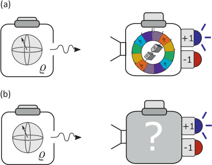
Figure 1: Concepts of randomised local measurements. A source (left box) emits a single qubit (spin-$1/2$ particle) in a specific and well-defined state every time the experimenter presses the button on the top of the box. The spin is measured by the measurement apparatus (right box) set in a random direction, obtaining one of the two possible outcomes $-1$ and $+1$. Pressing the button on the measurement apparatus randomly changes its measurement direction as illustrated by a wheel-of-fortune-driven Stern-Gerlach magnet in panel a). One distinguishes the cases where the experimenter knows the randomly chosen setting and where this information is not available, depicted by the question mark in panel b). While it is expected that one can estimate non-trivial features of the measured quantum system using the scenario in panel a), we highlight the possibility to learn a lot about the system, even when no information about each particular chosen setting is available to the experimenter, as illustrated in panel b). Note, however, that some information about the distribution of settings is required.

Let us begin by characterising more precisely what is meant by the term “randomised measurements”, which is sometimes used in different senses in the literature. In general, “randomness” has two aspects, a lack of control to choose a particular measurement setting and a lack of information about the chosen setting. A further distinction is the degree of fluctuation of the randomness, i.e. how much its effect varies with time or whether it is fixed. For illustration consider a model of the measurement of a quantum state by a single observer presented in Fig. 1. A source sends a single qubit prepared in a particular quantum state whenever the experimenter presses the top button at the source box. The same state is prepared each time the button is pressed. The qubit is then measured by an apparatus indicating the binary measurement outcome. Whenever the experimenter presses the top button on the measuring box, a new measurement setting is chosen randomly, i.e. the experimenter lacks control of the orientation of the subsequent setting. However, as in the case of Fig. 1a, it is still possible that the orientation of the randomly chosen setting is known, even if its choice cannot be controlled. The requirement for this knowledge is the existence of a reference frame which allows the observer to infer the relative orientation of the chosen settings in the space of possible settings. A simple practical example is a spatial coordinate system which allows to determine the orientation of spatially sensitive measurement devices in a lab. The situation in Fig. 1a is also an instance of fluctuating randomness, since the random orientation of the setting changes for each measurement.

Scenarios as these, where there is more information about the setting than control over it, give rise to a range of possibilities to analyse the state which were reviewed, among other scenarios, in Ref. [12]. For example, one can characterise complex quantum systems, estimate non-linear functions of the quantum states and also perform quantum tomography. Notably, the knowledge of the randomly selected measurement setting provides information about the measured state even when there is only one source emission per setting, i.e. the experimenter presses the button on the measurement box each time she presses the source button.

Interestingly, it is possible to obtain information about a physical system even when a reference frame is not available. In such a case the experimenter does not know the orientation of the randomly chosen settings, as depicted in Fig. 1b. Instead, information about the distribution of a set settings can be harnessed to obtain information about the state of a quantum system. Additionally, it is required to reliably estimate an expectation value for each randomly chosen (unknown) setting. This corresponds to pressing the source button in Fig. 1b) many times (to gather sufficient statistics) before pressing the button on the measurement box again to reorient the measurement direction. Crucially, this scenario does not require a lack of control which is independent of the lack of information. The absence of a reference frame is sufficient to account for the lack of control. Notably this scenario would even be random if the button would have no function, i.e. the state would remain at a fixed setting, such that "random" would simply denote a lack of information about the fixed orientation. This review focuses exclusively on scenarios as these, where randomness can be entirely viewed in terms of a lack of information and no recourse to control is necessary.

Table 1: Approaches to various types of randomised scenarios. This table summarises the various types of randomness classified according to the fluctuation of the randomness and the degree of alignment of reference frames. Any of these can be regarded as a “randomised measurement” scenario. Most of the entanglement detection techniques discussed in Sec. 3 rely on the measurement of product observables and are compatible with a complete absence of reference frame and fluctuating randomness. Additionally several local unitary invariant properties of states can be determined in this manner as discussed in Sec. 4. If local reference frames are available with only a fixed (or sufficiently slowly fluctuating) relative misalignment between observers, it is possible to also measure non-product observables, which can be applied to construct even stronger criteria for entanglement or determine a broader range of local unitary invariants. Finally, persistent misalignment allows to evaluate Bell-type inequalities with random settings to detect non-local correlations, as discussed in Sec. 5. However, also in a fluctuating scenario it is possible to verify that a state can produce non-local correlations without actually testing Bell-type inequalities, by considering average correlations which do not rely on a reference frame.

	Partial Alignment	Only Local Alignment	No Alignment
Fixed	Bell Violations (Sec. 5)	Non-Product Observables (Sec. 3,4) Bell Violations (Sec. 5)	Bell Violations (Sec.  5)
Fluctuating	-	-	Product Observables (Secs. 3,4) Average Correlation (Sec. 5)

For multipartite systems shared by several observers another point is the relative alignment of settings, i.e. the existence of a shared reference frame. Even if each observer has access to a reference frame, from now on denoted accordingly as local reference frame, still there might be unknown persistent or fluctuating rotations present between the particular frames of the observers. In some cases, these might only constitute a partial misalignment between the local frames, when for example in a multi-partite qubit state, observers share a single direction of the Bloch-sphere. In general, the establishing of a common reference frame is a physical process and in some practical scenarios, it is of interest to conserve the necessary physical resources [13, 14]. The various scenarios of randomness are summarised in Tab. 1 and classified according to the persistence of the randomness and the degree of availability of information about the setting.

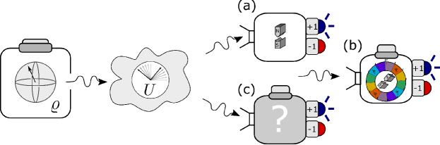
Figure 2: Randomness due to noisy environments. a) A measurement in a fixed basis following a random environment is effectively a randomised measurement. The randomly chosen measurement directions and their distribution remain unknown. Additional local rotations allow for measurements in a well defined local reference frame b) or alternatively for the removal of a possible bias in the distribution brought forward by the environment, through additional uniform noise c).

Randomised measurements can be implemented in an experiment on purpose or can appear naturally due to noisy environments. Note, that while some types of noise, such as decoherence or losses, do not correspond to random rotations of the reference frames, nevertheless there is a broad range of typically encountered environments, which can be modelled in very good approximation in this manner, formally expressed as unitary operations. Thus, the effects of these environments can be modelled by the transmission channel of the state containing a random unitary rotation, as illustrated in Fig. 2. These rotations can be fixed or fluctuating. However, even when fluctuations are present, they need to be slow enough as to allow the collection of sensible statistics with practically the same setting. In an approach which does not require a local reference frame, the experimenter does not need to press her button and a single fixed setting is sufficient to effectively perform a set of random measurements on the state, see Fig. 2a. The reason for this is that the unitary can be equivalently understood as acting on the state or acting on the setting and in general there is freedom whether to consider locally rotated states (fixed or fluctuating) or relative rotations of the local reference frames between the observers.

In other cases it can be crucial to add another set of local rotations after the unitary rotation induced by the environment. This can correspond for example to a scenario where the noisy environment disturbs the relative alignment between the local reference frames, but each observer still has to be able to choose from a set of local settings in a well-defined local reference frame, as shown in Fig. 2b. Alternatively, for example to counter a possible bias from the environment in the selection of measurement settings, one can additionally randomise the measurement setting by selecting the setting from a suitable unbiased distribution, even if the biased distribution is unknown, depicted in Fig. 2c. Typical experimental implementations of such transformations are rotated waveplates and polarisers in optical polarisation measurements, or laser driven transitions in ion trap-based experiments. In fact, the quantitative methods to analyse states with randomised measurements described here, rely on a uniform sampling of measurement settings. In contrast to such scenarios with random noise or controlled randomness, there exist also experimental situations in which it can be very difficult or resource intensive to perform this sampling in particular since the amount of settings to sufficiently approximate uniformity is growing exponentially with the system size. For such scenarios alternative techniques are available which allow to extract the same quantities via comparatively smaller sets of locally aligned measurements, so called designs.

In this review we present various approaches sorted according to the type of information they are able to extract from randomised measurements. In Sec. 2, we provide an intuitive introduction to the concept of randomised measurements based on a two-qubit example and introduce basic mathematical tools. In Sec. 3 we review various entanglement criteria in terms of correlations between randomised measurements. They provide necessary and sufficient conditions for entanglement in pure states and certain mixed states, and in general give rise to witnesses capable of detecting genuine multipartite entanglement, bound entanglement or distinguishing various classes of entangled states. In Sec. 4 we describe estimations of local unitary invariants such as purity. We also provide an overview of shadow tomography where randomised measurements play a crucial role. In Sec. 5 we review approaches to detect Bell non-local correlations between physical systems with randomised measurements. We discuss quantifiers such as the probability of violation and strength of non-locality, present common definitions of genuine multipartite non-locality, and scenarios where even with randomised measurements a violation of a Bell-type inequality is certain. We conclude in Sec. 6 and gather a list of interesting open problems encountered in the main body.

2 Randomised measurements in a nutshell

In this section, we explain basic formalism and give a brief overview of the possible applications of randomised measurements to the study of quantum systems. As an illustrative example, we start with the case of a two-qubit system and introduce the distributions of random correlation values as fundamental tools to investigate state properties. We identify the moments of these distributions as quantities which are straightforwardly accessible by randomised measurements and illustrate how they can be used in various criteria. The section includes several relevant concepts, such as quantum designs, sector lengths, local unitary invariants and PT moments. We conclude this section with a discussion of CHSH inequalities and the usefulness of Bell-type inequalities in the context of randomised measurements.

2.1 Distributions of correlation functions

To understand the general concept of randomised measurements and the difference in observations for entangled and separable states, let us first consider a simple two-qubit example with generalisations and extensions being discussed in subsequent sections. Assume we are given two states, a pure product state $|{\psi_{\mathrm{prod}}}\rangle\equiv|{\phi^{A}}\rangle\otimes|{\phi^{B}}\rangle$, that we will choose as $\left|00\right\rangle$, and an ideal Bell state, say a singlet state $\left|\psi^{-}\right\rangle=(\left|01\right\rangle-\left|10\right\rangle)/\sqrt{2}$, where we denote $\left|0\right\rangle=(1\ 0)^{\top}$, $\left|1\right\rangle=(0\ 1)^{\top}$, and abbreviate the tensor product as $\left|xy\right\rangle=\left|x\right\rangle\otimes\left|y\right\rangle$. The state $\left|\psi^{-}\right\rangle$ does not admit a product form. In fact, this property is a general definition of entanglement for any bipartite pure state. The two introduced states are now subjected to locally fluctuating randomised measurements. More precisely, many local projective measurements along randomly chosen measurement directions are performed such that a set of correlation values of the outcomes is obtained.

The correlation function is a statistical parameter characterising the statistical dependence of the results and is given by the mean of their product. In a two-qubit experiment, where the $j$-th particle (for $j=1,2$) is measured in a setting represented by the normalised vector $\mathbf{u}_{j}$ on the Bloch sphere, with a binary measurement outcome $r_{j}=\pm 1$, the correlation function reads

$$E(\mathbf{u}_{1},\mathbf{u}_{2})=\langle r_{1}r_{2}\rangle=\operatorname{\mathrm{tr}}\big{[}\varrho\;(\mathbf{u}_{1}\cdot\sigma\otimes\mathbf{u}_{2}\cdot\sigma)\big{]}.$$ (1)

The average is denoted here by $\langle\cdots\rangle$ and is in practice estimated by repeating the experiment sufficiently many times. The last expression in Eq. (1) represents the quantum mechanical prediction for the average measured given the system’s state $\varrho$. We use the short notation $\sigma$ for the vector of Pauli matrices, $\sigma=(\sigma_{x},\sigma_{y},\sigma_{z})$, that will also be conveniently enumerated as $(\sigma_{1},\sigma_{2},\sigma_{3})$, such that $\mathbf{u}_{j}\cdot\sigma$ is an arbitrary dichotomic observable, with outcomes $\pm 1$, of the $j$-th qubit. Such defined correlation functions are well known and feature, among other important applications, in violations of Bell inequalities.

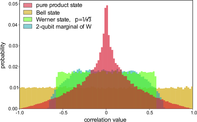
Figure 3: Numerically simulated probability distributions over values of the correlation function obtained under Haar-randomly chosen measurement directions. The results are shown for four different states indicated on the label. While the distributions are clearly distinct, states equivalent up to local unitary transformations result in equivalent distributions. The figure is taken from Ref. [15].

Consider now a scenario with a large amount of different, Haar randomly distributed measurements, i.e. directions that are distributed uniformly on a Bloch sphere. For more details and its generalisation see Sec. 3.2. For each randomly chosen set of measurement directions, the experiment is repeated sufficiently many times to obtain the correlation value arbitrarily close to the quantum prediction. Fig. 3 shows histograms of correlation values for different two-qubit states. A very different behaviour is observed for the Bell state (yellow) and the product state (red). For comparison, this figure also includes distributions for mixed entangled states, i.e. states which cannot be written in a separable form given by

$$\varrho^{AB}_{\text{sep}}=\sum_{i}p_{i}\varrho^{A}_{i}\otimes\varrho^{B}_{i},$$ (2)

where $p_{i}>0$ and $\sum_{i}p_{i}=1$. The two presented classes of mixed states are Werner states $\varrho_{\mathrm{Werner}}=(1-p)/4\leavevmode\nobreak\ {\mathbbm{1}}_{4}+p\left|\psi^{-}\right\rangle\left\langle\psi^{-}\right|$, and a two-qubit marginal of a $W_{3}$ state, that is $\varrho^{\mathrm{W_{3}}}_{2}=\operatorname{\mathrm{tr}}_{3}(\left|W_{3}\right\rangle\left\langle W_{3}\right|)$ with $\left|W_{3}\right\rangle=\left(\left|001\right\rangle+\left|010\right\rangle+\left|100\right\rangle\right)/\sqrt{3}.$ The data presented in Fig. 3 shows that the knowledge of the probability distribution of correlations contains valuable information characterising the state. Although this numerical simulation uses the ideal correlation values as described in Eq. (1), a finite amount of different measurement directions has been chosen, leading to, e.g. the deviations of the yellow distribution from a perfect uniform distribution.

It should be noted that, due to the nature of random measurements, states equivalent under local unitary (LU) transformations cannot be distinguished. For example, any maximally entangled two-qubit state gives rise to the same distribution of outcomes as the singlet state and every pure product state is indistinguishable from the product state used to compute the distribution in Fig. 3. This is not surprising since all entanglement properties are by definition LU invariant. We elaborate more about this in Sec. 2.6.

2.2 Moments of probability distributions

A glance at Fig. 3 shows that the difference between the Bell state $\left|\psi^{-}\right\rangle$ and the pure product state $|{\psi_{\mathrm{prod}}}\rangle$ is in the variances of their distributions. This immediately raises the question of whether a larger variance can in general imply entanglement. In the following, we expand on this intuition and formulate the corresponding entanglement criterion.

To proceed, let us define the moments of the probability distribution for the values of the correlation function as

$$\mathcal{R}^{(t)}(\varrho)=N_{t}\int\mathrm{d}\mathbf{u}_{1}\int\mathrm{d}\mathbf{u}_{2}\,[E(\mathbf{u}_{1},\mathbf{u}_{2})]^{t},$$ (3)

where $\mathrm{d}\mathbf{u}_{j}=\sin{\theta_{j}}\mathrm{d}\theta_{j}\mathrm{d}\phi_{j}$ denotes the measure on the unit sphere which is also the Haar measure, see Refs. [16, 17, 18]. Here, $N_{t}$ denotes a normalisation constant, which is chosen differently across the literature. The moments are invariant under any local unitary transformations of the state such that $\mathcal{R}^{(t)}(\varrho)=\mathcal{R}^{(t)}(V_{1}\otimes V_{2}\varrho V_{1}^{\dagger}\otimes V_{2}^{\dagger})$ for any single-qubit unitaries $V_{1},V_{2}$. Therefore, the moments seem especially suited to capture the correlation properties of $\varrho$, in the absence of local reference frames.

Note that $\mathcal{R}^{(t)}$ vanishes for odd $t$ since the sign of the correlation function is flipped under $\mathbf{u}_{j}\to-\mathbf{u}_{j}$. Indeed, as seen in Fig. 3, the expectation ($t=1$) is zero in all states. Thus, the first nontrivial result appears for $t=2$. As discussed in more detail in Sec. 3.4, the second moment gives rise to the following entanglement criterion:

$$\textrm{If }\mathcal{R}^{(2)}(\varrho)>1,\textrm{ then }\varrho\textrm{ is entangled.}$$ (4)

This result is illustrated in Fig. 3, where the Bell state has a large variance compared to the pure product state.

We should stress that the criterion (4) is only sufficient but not necessary for mixed two-qubit entangled states. That is, there exist mixed entangled states that this criterion cannot detect. Examples are the Werner states $\varrho_{\mathrm{Werner}}$ for $1/3<p\leq 1/\sqrt{3}$, and the two-qubit marginal of the $W_{3}$, state $\varrho^{\mathrm{W_{3}}}_{2}$. To distinguish between these states and detect a broader range of entanglement, we need to use higher moments ($t>2$) to construct more refined entanglement criteria. The details will be discussed in Secs. 3.5 and 3.6.

2.3 Quantum designs

In order to evaluate the uniform average over the sphere in Eq. (3), the concept of designs is very helpful. Consider a polynomial function $P_{t}(\mathbf{x})$ in $n$ variables with degree $t$. We call a set $X=\{\mathbf{x}_{j}\in S_{n}\}_{j=1,\ldots,K}$ spherical $t$-design if

$$\frac{1}{K}\sum_{\mathbf{x}_{j}\in X}P_{t}(\mathbf{x}_{j})=\int\mathrm{d}\mathbf{x}\,P_{t}(\mathbf{x}),$$ (5)

where $\mathrm{d}\mathbf{x}$ is the spherical measure on the $n$-dimensional unit sphere $S_{n}$ with $\int\mathrm{d}\mathbf{x}=1$ [19, 20]. That is, the integral for any polynomial of at most degree $t$ can be evaluated by knowing the value of the polynomial at $K$ discrete points $\mathbf{x}_{j}$ of the spherical $t$-design set $X$. By definition, the integral at the right-hand side in Eq. (5) is invariant under any rotation on the sphere, so the evaluated expression on the left-hand side is also invariant. In general, if the allowed degree $t$ or the dimension $n$ increases, then a larger set $X$ is required. The details will be discussed in Sec. 3.3.

To give a concrete example, let us evaluate the second moment $\mathcal{R}^{(2)}$ using the idea of spherical designs. This corresponds to the case $t=n=2$. It is well known that a set of $K=6$ unit vectors on orthogonal antipodals, $\{\mathbf{x}_{j}=\pm\mathbf{e}_{j}:j=x,y,z\}$, where $\mathbf{e}_{j}$ are the Cartesian axes, is a spherical $2$-design (and also $3$-design) [18, 21, 22]. Using this spherical design, we rewrite each of the two integrals in $\mathcal{R}^{(2)}$ over a two-dimensional unit sphere as the average over the set of six points on the sphere:

$$\mathcal{R}^{(2)}(\varrho)=3^{2}\frac{1}{6^{2}}\sum_{j,k=1}^{6}[E(\mathbf{e}_{j},\mathbf{e}_{k})]^{2}=\sum_{j,k=x,y,z}[\operatorname{\mathrm{tr}}(\varrho\;\sigma_{j}\otimes\sigma_{k})]^{2},$$ (6)

where we choose the normalisation $N_{2}=(3/4\pi)^{2}$ and use the fact that the even function $[E(\mathbf{u}_{1},\mathbf{u}_{2})]^{2}$ does not change under the sign flip. As a result, the integral over the entire spheres $\mathbf{u}_{1},\mathbf{u}_{2}$ is replaced by a sum of nine (squared) correlation functions computed along orthogonal directions on local Bloch spheres. Note that higher moments may be found in a similar manner, using designs for larger $t$. Recalling that $\mathcal{R}^{(2)}$ is LU invariant and a convex function of a state, the separability bound can be found, without loss of generality, by considering the pure product state $|{\psi_{\mathrm{prod}}}\rangle=\left|00\right\rangle$. We therefore arrive at the criterion discussed in the last section, $\mathcal{R}^{(2)}(\varrho_{\text{sep}})\leq 1$ for any two-qubit separable state $\varrho_{\text{sep}}$.

2.4 Bloch decomposition of multipartite quantum states

Any single-qubit state $\varrho_{A}$ can be expressed using the operator basis of Pauli matrices as

$$\varrho_{A}=\frac{1}{2}\left(\mathbbm{1}_{2}+a_{x}\sigma_{x}+a_{y}\sigma_{y}+a_{z}\sigma_{z}\right).$$ (7)

Since Paulis are traceless the overall factor of $1/2$ follows from normalisation $\operatorname{\mathrm{tr}}(\varrho_{A})=1$. The positive semidefiniteness of the state $\varrho_{A}$ is equivalent to the constraint $\sum_{j=x,y,z}a_{j}^{2}\leq 1$ [23]. The parametrisation in Eq. (7) enables us to visualise the state as a point within a unit sphere in a three-dimensional space with coordinates ${\textbf{a}}=(a_{x},a_{y},a_{z})$. It is called the Bloch sphere and has the property that a pure state corresponds to a point on the surface of the sphere, while a mixed state corresponds to a point inside. It is essential to note that the length of its radius, denoted as $L(\varrho)=\sum_{j=x,y,z}a_{j}^{2}$, corresponds to the purity $\mathcal{P}(\varrho)=\operatorname{\mathrm{tr}}(\varrho^{2})$, which remains invariant under unitary rotations. That is, $0\leq L(\varrho)=L(U\varrho U^{\dagger})\leq 1$, where the first and second inequalities are respectively saturated by the completely mixed state and pure states.

The decomposition in terms of Pauli operators $\{\mathbbm{1}_{2},\sigma_{x},\sigma_{y},\sigma_{z}\}$ Eq. (7) is based on the relation $\operatorname{\mathrm{tr}}(\sigma_{\mu}\sigma_{\nu})=2\delta_{\mu\nu}$ for $\mu,\nu=0,1,2,3$. In the same way, a tensor product of Pauli operators forms a basis for composite quantum states. For example, we can represent a two-qubit state $\varrho_{AB}$ in the Bloch form

$$\varrho_{AB}=\frac{1}{4}\left(\mathbbm{1}_{2}^{A}\otimes\mathbbm{1}_{2}^{B}+\sum_{j=x,y,z}a_{j}\sigma_{j}^{A}\otimes\mathbbm{1}_{2}^{B}+\sum_{j=x,y,z}b_{j}\mathbbm{1}_{2}^{A}\otimes\sigma_{j}^{B}+\sum_{j,k=x,y,z}T_{jk}\sigma_{i}^{A}\otimes\sigma_{k}^{B}\right),$$ (8)

with $\sigma_{j}^{A}\in\mathcal{H}_{2}^{A}$ and $\sigma_{j}^{B}\in\mathcal{H}_{2}^{B}$ for $j=x,y,z$. The coefficients $a_{j}$ and $b_{j}$ describe the reduced states, whereas the so-called correlation tensor $T=(T_{jk})$ captures two-body quantum correlations. Here, the positivity of $\varrho_{AB}$ implies several non-trivial constraints on the possible values of $\{a_{j},b_{j},T_{jk}\}$. Thus in general it is difficult to find the complete set of values satisfying these constraints. The simplest example is given by $\sum_{j=x,y,z}(a_{j}^{2}+b_{j}^{2})+\sum_{j,k=x,y,z}T_{jk}^{2}\leq 3$ from the purity condition $\operatorname{\mathrm{tr}}(\varrho_{AB}^{2})\leq 1$, for details see Refs. [24, 25, 26, 27]. Notice that Eq. (6) can be written as $\mathcal{R}^{(2)}(\varrho_{AB})=\sum_{j,k=x,y,z}T_{jk}^{2}$. Thus the sufficient criterion for two-qubit entanglement reads: if $\sum_{j,k=x,y,z}T_{jk}^{2}>1$, then the state is entangled.

The Bloch decomposition can be generalised to $n$-particle $d$-dimensional quantum states ($n$-qudits) with

$$\varrho=\frac{1}{d^{n}}\sum_{j_{1},\cdots,j_{n}=0}^{d^{2}-1}T_{j_{1}\cdots j_{n}}\lambda_{j_{1}}\otimes\cdots\otimes\lambda_{j_{n}},$$ (9)

where $\lambda_{0}$ is the identity $\mathbbm{1}_{d}$, and $\lambda_{j}$ are the normalised Gell-Mann matrices, such that $\lambda_{j}=\lambda_{j}^{\dagger}$, $\mathrm{tr}[\lambda_{j}\lambda_{k}]=d\delta_{j,k}$, and $\mathrm{tr}[\lambda_{j}]=0$ for $j>0$ [28, 29]. The correlation tensor $T_{j_{1}\cdots j_{n}}$ was essentially first considered by Schlienz and Mahler in Ref. [30]. Note that some references use different normalisation of the $\lambda_{j}$ or yet different bases such as, for example, the Heisenberg-Weyl matrices [31, 32]. We remark that the $k$-fold tensor $T_{j_{1}\cdots j_{n}}$ for $1\leq k\leq n$, i.e. the entries, for which $k$ indices are non-zero, characterises the $k$-body correlations of the (reduced) state.

2.5 Sector lengths

The Bloch representation directly leads to the notion of so-called sector lengths. As mentioned, the length of the one-party Bloch vector quantifies the degree of mixing of the state. Accordingly, the length encodes information about the state that can be obtained in a basis-independent way. The sector lengths are its direct extension to multipartite quantum systems.

To proceed, recall the generalised Bloch decomposition of a $n$-qudit state in Eq. (9). Sector lengths are defined as follows [33]:

$$S_{k}(\varrho)=\sum_{k\textrm{ non-zero indices}}T_{j_{1}\cdots j_{n}}^{2},$$ (10)

where $S_{0}=\lambda_{0\cdots 0}=1$ due to the normalisation condition $\operatorname{\mathrm{tr}}(\varrho)=1$. The sector lengths $S_{k}$ quantify the amount of $k$-body correlations in the state $\varrho$. For example, in the case of the three-qubit GHZ state $\left|\mathrm{GHZ}_{3}\right\rangle=(\left|000\right\rangle+\left|111\right\rangle)/\sqrt{2}$, one obtains $(S_{1},S_{2},S_{3})=(0,3,4)$. Additionally, note that Eq.( 4) along with ( 6) give an entanglement criterion in terms of sector length.

Sector lengths have several useful properties. (i) The sector lengths are invariant under any local unitary transformation. That is, for a local unitary $V_{1}\otimes\cdots\otimes V_{N}$, it holds that $S_{k}(\varrho)=S_{k}\big{(}V_{1}\otimes\cdots\otimes V_{n}\varrho V_{1}^{\dagger}\otimes\cdots\otimes V_{n}^{\dagger}\big{)}$. (ii) The sector lengths are convex on quantum states. That is, for the mixed quantum state $\varrho=\sum_{i}p_{i}\left|\psi_{i}\right\rangle\!\left\langle\psi_{i}\right|$, it holds that $S_{k}\left(\sum_{i}p_{i}\left|\psi_{i}\right\rangle\!\left\langle\psi_{i}\right|\right)\leq\sum_{i}p_{i}S_{k}(\left|\psi_{i}\right\rangle)$. (iii) The sector lengths have a convolution property: For a $n$-particle product state $\varrho_{P}\otimes\varrho_{Q}$, where $\varrho_{P}$ and $\varrho_{Q}$ are, respectively, $j$-particle and $(n-j)$-particle states, we have $S_{k}(\varrho_{P}\otimes\varrho_{Q})=\sum_{i=0}^{k}S_{i}(\varrho_{P})S_{k-i}(\varrho_{Q})$ [26]. (iv) The sector lengths are directly associated with the purity of $\varrho$, namely

$$\mathcal{P}(\varrho)=\frac{1}{d^{n}}\sum_{k=0}^{n}S_{k}(\varrho).$$ (11)

That is, the purity can be decomposed into the sector lengths of different orders. Using this relation, the sector lengths can be always represented as the purities of reduced states of $\varrho$, and vice versa. (v) The $n$-body (often called full-body) sector length $S_{n}$ for all $n$-qubit states has been shown to be always maximised by the $n$-qubit GHZ state, denoted by $\left|\text{GHZ}_{n}\right\rangle=(\left|0\right\rangle^{\otimes n}+\left|1\right\rangle^{\otimes n})/\sqrt{2}$. Its maximal value is given by $S_{n}(\text{GHZ}_{n})=2^{n-1}+\delta_{n,\,\text{even}}$ [17, 34, 35]. However, this is not always true in higher dimensions, i.e. quantum states that are not of the GHZ form can attain the maximal $S_{n}$ value [34]. Even more interestingly, it has been demonstrated that there exist multipartite entangled states with zero $S_{n}$ for an odd number of qubits [36, 37, 38, 39, 40].

Finally and importantly, the sector lengths can be directly obtained from the randomised measurement scheme. In fact, the $k$-body sector lengths $S_{k}$ can be represented as averages over all second-order moments of random correlations in $k$-particle subsystems. The entanglement criteria using the sector lengths are therefore accessible with randomised measurements, for details see Sec. 3.7.

2.6 Local unitary invariants

Moments of random correlations and sector lengths are special cases of a broader class of the quantum state functions which are invariant under local unitary transformations. In general, such local unitary (LU) invariants $q(\varrho)$ are functions of the quantum state $\varrho$ for which

$$q\big{(}V_{1}\otimes\cdots\otimes V_{n}\varrho V_{1}^{\dagger}\otimes\cdots\otimes V_{n}^{\dagger}\big{)}=q(\varrho),$$ (12)

for any $V_{1}\otimes\cdots\otimes V_{n}$ with $V_{i}$ defined in a $d$-dimensional unitary group. Since the purity of the global state $\mathcal{P}(\varrho)=\operatorname{\mathrm{tr}}(\varrho^{2})$ is invariant under any global unitary, one can interpret the relation in Eq. (11) as a decomposition of a global unitary invariant into LU invariants. Moreover, for two qubits $\operatorname{\mathrm{tr}}(\varrho^{3})$, can be expressed with the help of the determinant $\det{(T)}$ of the correlation tensor introduced in Eq. (8). This is one of the so-called Makhlin LU invariants [41].

Here a nontrivial question arises: How can we access certain LU invariants from randomised measurements? Since LU invariants include detailed information about quantum correlations in the state, addressing this question can be related to the improvement of entanglement detection and can reveal many other important properties of the state. In Secs. 3.5.2 and 4.3, we discuss how LU invariants for two qubits can be characterised by randomised measurements.

Another example of LU invariant is the Rényi entropy of order $\alpha$, defined as

$$H_{\alpha}\left(\varrho_{M}\right)=\frac{1}{1-\alpha}\log\left[\operatorname{\mathrm{tr}}\left(\varrho_{M}^{\alpha}\right)\right],$$ (13)

where $\alpha\in\mathbb{R},\alpha\neq 0,\alpha\neq 1$, the reduced state is defined as $\varrho_{M}=\operatorname{\mathrm{tr}}_{\bar{M}}(\varrho)$ for any $M=\{1,2,\ldots,n\}$ and the trace is taken over the complement $\bar{M}$. In particular, the second-order Rényi entropy $H_{2}$ is often used to analyse entanglement [42]. This quantity is accessible through randomised measurements, see Secs. 3.6.1 and 4.1.

2.7 PT moments

A different route to witnessing entanglement via randomised measurements is based on the Peres-Horodecki separability criterion [43, 44]. It states that if a bipartite state $\varrho_{AB}$ is separable, then the partially transposed density matrix $\varrho^{\Gamma_{B}}_{AB}:=(\text{id}\otimes T)(\varrho_{AB})$ is positive semi-definite, where id is the identity map and $T$ is the transposition map. States with this property are called PPT states, as they have a positive semidefinite partial transpose. Contrary, if $\varrho^{\Gamma_{B}}_{AB}$ has negative eigenvalues, the state is called NPT and must be entangled. Importantly, for systems consisting of two qubits or a qubit and a qutrit a positive semi-definite $\varrho^{\Gamma_{B}}_{AB}$ is also a sufficient criterion for separability. In general, however, there exist entangled states that the PPT criterion can never detect. The criterion can also be used to quantify entanglement and the corresponding entanglement monotone is provided by the logarithmic negativity defined as [45, 46, 47, 48, 49]

$$\mathrm{E}_{N}(\varrho_{AB})=\log||\varrho_{AB}^{\Gamma_{B}}||_{1}=\log\sum_{i}|\lambda_{i}|,$$ (14)

with $||\cdot||_{1}$ being the trace norm and $\lambda_{i}$ the eigenvalues of the partially transposed density matrix.

In order to make the PPT criterion accessible by randomised measurements one considers the so-called PT (or negativity) moments. The $k$-th PT moment is defined as

$$p_{k}(\varrho_{AB})=\operatorname{\mathrm{tr}}\left[\left(\varrho_{AB}^{\Gamma_{B}}\right)^{k}\right].$$ (15)

These quantities are LU invariant for any order $k$, since the eigenvalues of the partially transposed matrix are LU invariant. Similarly to the moments of the given density matrix [see their use in Eq. (13)], these moments can be determined by randomised measurements [50, 51], as described in Sec. 4.2.

Furthermore, it is a well-established mathematical fact that the coefficients of the characteristic polynomial of a matrix can be expressed in terms of traces of the power of this matrix [52], so knowledge of the moments $p_{k}$ for any $k$ allows to evaluate the PPT criterion. In practice, however, only a few of these moments can be measured and the question arises: Is this data compatible with a PPT density matrix or not? This question is similar to security analysis in entanglement-based quantum key distribution, where the protocol is insecure, if the measured data is compatible with a separable state [53].

In Ref. [54] it was shown via a machine-learning approach that the logarithmic negativity can be estimated using $p_{3}$. As an analytical result, the following moment-based entanglement criterion was introduced in Ref. [51],

$$p_{3}<p_{2}^{2}\implies\mbox{$\varrho_{AB}$ is NPT and hence entangled.}$$ (16)

This so-called $p_{3}$-PPT criterion was utilised to detect entanglement in the experimental data from Ref. [55]. It is worth noting that the PT-moment approach, even with lower orders, can detect the Werner state in a necessary and sufficient manner for any dimension, for more details see Appendix in Ref. [51].

Still, the $p_{3}$-PPT criterion is not the optimal way to extract information from the moments $p_{2}$ and $p_{3}.$ This problem can be solved with a family of optimal criteria ($p_{n}$-OPPT) derived in Ref. [56], see also Ref. [57]. For the special case of $n=3$, the necessary and sufficient $p_{3}$-OPPT condition for compatibility of the PT moments with a PPT state is given by

$$p_{3}\geq\alpha x^{3}+(1-\alpha x)^{3},$$ (17)

where $\alpha=\lfloor 1/p_{2}\rfloor$ and $x=[\alpha+(\alpha[p_{2}(\alpha+1)-1])^{1/2}]/[\alpha(\alpha+1)]$. Note that the above expression does not depend on the Hilbert space dimension. Also, if the PT moments are compatible with the spectrum of a PPT state, they are compatible with a separable state, since one can directly write down a separable state (diagonal in the computational basis) for a given nonnegative spectrum of the partial transpose. Finally, the $p_{n}$-OPPT criteria are defined for all $n\geq 3$ and demonstratively stronger than their $p_{n}$-PPT counterparts as shown with numerical simulations [56].

2.8 Bell-type inequalities

Another topic where randomised measurements are highly useful tools is tests of non-local correlations in quantum systems. One of the most fundamental properties of quantum mechanics is that measurement results at spatially separated measurement sites exhibit correlations that do not permit a classical description. As shown by Bell’s theorem [58, 59] such correlations can only be explained if certain fundamental assumptions about the physical world are given up. These include relativistic causality, the possibility to choose measurement settings independently of the experimental results or the ability to causally explain the occurrence of the outcomes altogether, sometimes also referred to as giving up “realism”, for a careful analysis see [60]. Apart from such basic questions, this class of correlations is also an important resource used in numerous quantum information processing protocols, in particular in quantum key distribution [61], in the certified generation of unpredictable randomness [62], and in reducing the communication complexity of computation [63]. These unique properties of quantum systems are sometimes called “quantum nonlocality” or “Bell non-locality” in the literature [64, 65].

Whether a given state produces Bell non-locality is usually tested via inequalities which give bounds on functions of expectation values for joint measurements at spatially separated sites sharing an entangled state [65, 64]. The simplest of these, the Clauser-Horne-Shimony-Holt (CHSH) inequality [66] applies to the scenario of two observers who share an entangled state of two qubits. They perform dichotomic measurements, with the first observer choosing between two alternative observables $\mathbf{u}_{1}\cdot\sigma$ and $\mathbf{u}_{1}^{\prime}\cdot\sigma$, and the second observer between $\mathbf{u}_{2}\cdot\sigma$ and $\mathbf{u}_{2}^{\prime}\cdot\sigma$. It can be proven that any Bell-local model [67], i.e. any model respecting all assumptions of Bell’s theorem, satisfies the inequality

$$|E(\mathbf{u}_{1},\mathbf{u}_{2})+E(\mathbf{u}_{1},\mathbf{u}_{2}^{\prime})+E(\mathbf{u}_{1}^{\prime},\mathbf{u}_{2})-E(\mathbf{u}_{1}^{\prime},\mathbf{u}_{2}^{\prime})|\leq 2.$$ (18)

For a suitable maximally entangled state and an optimal choice of observables as for example $\mathbf{u}_{1}=\mathbf{x}$, $\mathbf{u}_{1}^{\prime}=\mathbf{z}$, and $\mathbf{u}_{2}=(\mathbf{x}+\mathbf{z})/\sqrt{2}$, $\mathbf{u}_{2}^{\prime}=(\mathbf{x}-\mathbf{z})/\sqrt{2}$ we obtain the largest value of the left-hand side of the inequality $S_{max}=2\sqrt{2}>2$ and hence the maximal violation of the inequality. The quantum violations of similar inequalities have been observed in precisely dedicated experiments [68, 69, 70, 71].

One can also ask if a Bell-local model exists when the CHSH inequality is not violated. The answer is negative and a necessary and sufficient condition for the existence of such a model is given by a set of inequalities (not just one of them) which describe the facets of so-called Bell-Pitowsky polytope [72]. These polytopes are different for scenarios with different numbers of observers, measurement settings and outcomes. It turns out that for two parties, each choosing between two dichotomic measurements, it is sufficient to permute the observables in the CHSH inequality to generate the complete set of 16 CHSH inequalities describing the Bell-Pitowsky polytope. For more complex scenarios the corresponding polytopes have been fully characterised analytically only for special cases [73, 74, 75, 76, 77, 78].

The maximum value $S$ of the CHSH expression that a given state $\varrho$ can achieve, optimised over the choice of measurements, is given by $S(\varrho)=2\sqrt{\lambda_{1}+\lambda_{2}}$, where $\lambda$’s are the two largest eigenvalues of the matrix $T^{\top}T$ [79] with $T$ defined in Eq. (8). The corresponding state violates the CHSH inequality if and only if $\sqrt{\lambda_{1}+\lambda_{2}}>1$. This condition can also be expressed directly in terms of correlation matrix elements [80] as $\sum_{i,j=x,y}T_{ij}^{2}>1$, where the axes $x$ and $y$ define the plane in which the optimal settings for the inequality lie.

While, in general, a particular choice of settings is crucial to obtain the violation of Bell-type inequalities such as the CHSH inequality, it is interesting to investigate whether Bell non-local correlations can also be witnessed in the scenario of randomised measurements. Interestingly, it turns out that with suitable states a violation can still be guaranteed, even if certain fixed random rotations are added between the reference frames of the two observers or even with randomness in the local frames. A detailed discussion of this topic will be presented in  Secs. 4.3 and 5.

3 Entanglement

In this section, we summarise several results on detecting entanglement using randomised measurements. We begin with an introduction to the theory of entanglement and the general framework of randomised measurements focusing on the $t$-th moment of the distributions of correlation values in multipartite high-dimensional systems. We also provide an overview of quantum $t$-designs as a powerful tool for the computation of integrals over Haar randomly distributed unitaries. Subsequently, several applications of these tools are discussed to detect and characterise entanglement in a broad range of scenarios. The section concludes with a discussion of the effects of statistical noise due to limited data in experimental situations and proper strategies to account for this noise when applying the tools presented before.

3.1 Multipartite entanglement

In the previous section, basic intuitions behind the structure of entanglement and its detection with randomised measurements have been introduced. Here, we discuss entanglement beyond the two-qubit scenario to include systems with an arbitrary dimension and number of parties. The interested reader can find more details about the field of multipartite entanglement in several in-depth review articles [81, 82, 83, 84, 85, 86, 87].

An $n$-partite $d$-dimensional quantum state ($n$-qudit) defined in the Hilbert space $\mathcal{H}_{d}^{\otimes n}$ is fully separable if it can be written as

$$\varrho_{\text{fs}}=\sum_{i}p_{i}\varrho_{i}^{1}\otimes\varrho_{i}^{2}\otimes\cdots\otimes\varrho_{i}^{n},$$ (19)

where $\varrho_{i}^{j}$ are quantum states and the $p_{i}$ form a probability distribution, i.e. $p_{i}\geq 0$ and $\sum_{i}p_{i}=1$. We say that a $n$-particle state contains entanglement if it is not fully separable. Note, that this does not imply anything about the structure of the entanglement, as for example whether all parties are entangled with each other. One option to intuitively understand different types of entanglement is to consider how states are prepared. For instance, $\varrho_{\text{fs}}$ can be prepared from a product state by local operations and classical communication (LOCC) by operating on each particle separately. One can also consider states which can be prepared from a product state by LOCC where the operations are performed jointly on groups of particles (not just on one particle).

For instance, a state is called biseparable with respect to a bipartition $M|\bar{M}$ for a subset $M\subset\{1,2,\ldots,n\}$ if it can be written as

$$\varrho_{M|\bar{M}}=\sum_{i}q_{i}^{M}\varrho_{i}^{M}\otimes\varrho_{i}^{\bar{M}},$$ (20)

where the $q_{i}^{M}$ form a probability distribution, $\bar{M}$ is the complement of $M$ and $\varrho_{i}^{M}$ is a quantum state of particles in set $M$. In order to prepare state $\varrho_{M|\bar{M}}$ via LOCC one needs to operate jointly on subsystems in the set $M$ and in the set $\bar{M}$. Moreover, one can consider mixtures of biseparable states for all bipartitions,

$$\varrho_{\text{bs}}=\sum_{M}p_{M}\varrho_{M|\bar{M}},$$ (21)

where $p_{M}$ are probabilities and the summation includes at most $2^{n-1}-1$ terms. Such a general state is simply called biseparable (without reference to any concrete bipartition). A quantum state which cannot be written in the form (21) is called genuine $n$-particle entangled and involves entanglement between all subsystems.

For example, a three-particle state is called biseparable for a bipartition $A|BC$ if

$$\varrho_{A|BC}=\sum_{i}q_{i}^{A}\varrho_{i}^{A}\otimes\varrho_{i}^{BC},$$ (22)

where $\varrho_{i}^{BC}$ may be entangled. We can furthermore construct mixtures of biseparable states with respect to different partitions, i.e. states of the form

$$\varrho_{\text{bs}}=p_{A}\varrho_{A|BC}+p_{B}\varrho_{B|CA}+p_{C}\varrho_{C|AB},$$ (23)

where the $p_{A},p_{B},p_{C}$ are probabilities. In contrast, a typical example of a genuine $n$-qudit entangled state is the generalised Greenberger–Horne–Zeilinger (GHZ) state given by

$$\left|\text{GHZ}(n,d)\right\rangle=\frac{1}{\sqrt{d}}\sum_{i=0}^{d-1}\left|i\right\rangle^{\otimes n}.$$ (24)

In particular, in two-qudit systems (that is, $n=2$), this state is the maximally entangled two-particle state. Other examples of genuine $n$-partite entangled states include W states [88], Dicke states [89], cluster states [90], graph states [91], and absolutely maximally entangled (AME) states [92, 93, 94].

The question of whether a given quantum state is separable or entangled is known as the separability problem and is central for quantum information theory. It has several aspects:

• Even if the density matrix is completely known, in general it remains a complicated mathematical problem to determine whether a state is entangled, known to belong to the NP-hard class of computational complexity [95]. Following the Choi-Jamiolkowski isomorphism, connecting quantum states and channels [96, 97, 98, 99], the separability problem is equivalent to the problem of distinguishing positive and completely positive maps which is as yet unsolved.

• In experiments, sometimes only partial information about the state is accessible. If some a priori information about the state is available, e.g. that an experiment is aimed at producing a certain entangled state, then so-called entanglement witnesses may allow for the efficient detection using directly measurable observables [99, 100, 81]. In other situations, where one cannot be sure about the appropriate description of measurements and cannot trust the underlying quantum devices, it is still possible to certify entanglement in a device-independent manner [101], using, e.g. Bell-type inequalities, based only on the measurement data observed from input-output statistics [102, 103]. Moreover, when considering ensembles of quantum particles, such as cold atoms, individual control over local subsystems may be lost, but entanglement can still be characterised by measuring collective angular momenta and applying spin squeezing inequalities [104, 105, 106].

• Addressing the separability problem can highlight distinctions between quantum physics and classical physics in terms of correlations. The features of entanglement, such as the negativity of conditional entropy [107, 108], monogamy of entanglement [109, 110], and the presence of bound entanglement [111, 112], are associated with entanglement conditions from fundamental and operational viewpoints. In fact, whether a given entangled state is useful or not, can be decided by certain thresholds in terms of several quantum communication protocols [113, 53, 114] and quantum metrology [115, 116, 117].

• As a generalisation of the separability problem, one can ask, for example, how many partitions are separated in a multipartite state based on the concept of $k$-separability [118, 119] (see Sec. 3.7.2), or how many particles are entangled based on the concept of $k$-producibility [120, 121, 122, 123]. Other interesting concepts are given by $k$-stretchability [124, 125, 126], tensor rank [127], and the bipartite and multipartite dimensionality [128, 129, 130] of entanglement. Genuine multipartite entanglement can in turn again be classified into several types, such as the W class or GHZ class of states, for details see Sec. 3.7.5. More recently, also different notions of network entanglement came into the focus of attention [131, 132, 133].

3.2 Randomised measurements on multipartite systems

While in Section 2 we have mainly discussed the second moment of correlations obtained via randomised measurements on two qubits, in the following we generalise this scheme to $t$-th moments in $n$-particle $d$-dimensional quantum systems. Using this formulation, we will review several systematic methods to detect various types of entanglement.

When measuring an observable $\mathcal{M}$ on a state with $n$ parties, $\varrho\in\mathcal{H}_{d}^{\otimes n}$, such that each party rotates their measurement direction in an arbitrary manner according to a randomly chosen unitary matrix $U_{i}$, the corresponding correlation function reads

$$E(\mathcal{M},U_{1}\otimes U_{2}\otimes\cdots\otimes U_{n})=\operatorname{\mathrm{tr}}\left[\varrho(U_{1}\otimes U_{2}\otimes\cdots\otimes U_{n})^{\dagger}\mathcal{M}(U_{1}\otimes U_{2}\otimes\cdots\otimes U_{n})\right].$$ (25)

This correlation function depends not only on $\varrho$ and $\mathcal{M}$ but also on the choice of local unitaries $U_{1}\otimes U_{2}\otimes\cdots\otimes U_{n}$. Here the unitary matrix $U_{i}$ is defined in the $d$-dimensional unitary group acting on the $i$-th subsystem for $i=1,2,\ldots,n$. By sampling random unitaries uniformly from the unitary group, the resulting distribution of the correlation functions can be characterised by its moments with

$$\mathcal{R}^{(t)}_{\mathcal{M}}(\varrho)=N_{n,d,t}\int\mathrm{d}\mu(U_{1})\int\mathrm{d}\mu(U_{2})\cdots\int\mathrm{d}\mu(U_{n})\,[E(\mathcal{M},U_{1}\otimes U_{2}\otimes\cdots\otimes U_{n})]^{t},$$ (26)

where the integral is taken according to the Haar measure $\mathrm{d}\mu(U)$. Here, we denote $N_{n,d,t}$ as a suitable normalisation constant, which is defined differently across the literature. For the case of $n=d=2$ we arrive at the form of Eq. (3) independently of which Pauli product observable $\mathcal{M}=\sigma_{i}\otimes\sigma_{j}$ with $i,j=x,y,z$ is chosen. In the same manner, without loss of generality the observable can be assumed to be $\sigma_{z}\otimes\sigma_{z}\otimes\ldots\sigma_{z}$ also for larger $n$.

To explain the properties of the moments, let us recap the notion of the Haar unitary measure. Let $\mathcal{U}(d)$ be the group of all $d\times d$ unitaries and $f(U)$ be a function on $U\in\mathcal{U}(d)$. Consider an integral of $f(U)$ over the unitary group $\mathcal{U}(d)$ with respect to the Haar measure $\mathrm{d}\mu(U)$. One of the most important properties of the Haar measure is the left and right invariance under shifts via multiplication by a unitary $V\in\mathcal{U}(d)$, which is respectively given by

$$\int\mathrm{d}\mu(U)\,f(U)=\int\mathrm{d}\mu(U)\,f(VU)=\int\mathrm{d}\mu(U)\,f(UV),$$ (27)

see Refs. [134, 135, 136, 137, 138] for further details. A general parametrization of the unitary group $\mathcal{U}(d)$ and the associated Haar measure are known [136, 139]. For instance, any single-qubit unitary ($d=2$) can be written in the Euler angle representation [140] as $U(\alpha,\beta,\gamma)=U_{z}(\alpha)U_{y}(\beta)U_{z}(\gamma)$, where $U_{i}(\theta)=e^{-i\theta\sigma_{i}/2}$ for $i=y,z$ and the Haar measure $\mathrm{d}\mu(U)=\sin(\beta)\mathrm{d}\alpha\mathrm{d}\beta\mathrm{d}\gamma$. By their definition, the moments are invariant under any local unitary transformation. More precisely, since the Haar measure is invariant under left and right translation, it holds that

$$\mathcal{R}^{(t)}_{\mathcal{M}}(\varrho)=\mathcal{R}^{(t)}_{\mathcal{M}}(V_{1}\otimes\cdots\otimes V_{n}\;\varrho\;V_{1}^{\dagger}\otimes\cdots\otimes V_{n}^{\dagger}),$$ (28)

for any local unitary $V_{1}\otimes\cdots\otimes V_{n}$. Thus, we can characterise the state $\varrho$ with the moments $\mathcal{R}^{(t)}(\varrho)$ in a local-basis-independent manner, that is, independent of reference frames between parties or unknown local unitary noise. This invariance is one of the most important properties of randomised measurements and suggests that the moments of the measured distributions contain essential information about the entanglement of the corresponding quantum states.

In general, the observable $\mathcal{M}$ does not necessarily have to be a product observable of the form $\mathcal{M}_{\text{P}}=M_{1}\otimes M_{2}\otimes\cdots\otimes M_{n}$, but can be of the more general form $\mathcal{M}_{\text{NP}}=\sum_{i}m_{i}M_{1}^{i}\otimes M_{2}^{i}\otimes\cdots\otimes M_{n}^{i}$, with real coefficients $m_{i}$ [141, 142]. The measurement of non-product observables requires a certain restriction of randomness, where the unitary cannot change significantly while the various observers switch between the particular local observables $M^{i}_{k}$ in a synchronised manner. However, as a tradeoff, it enables the extraction of additional information not accessible via product observables as discussed in Sec. 3.5 and also Secs.4.3 and 4.2.

By discarding the measurements of some parties, one can obtain the marginal moments of the reduced states of $\varrho$. For illustration, let us consider a three-particle state $\varrho_{ABC}$ and discard the measurements of the parties $B$ and $C$, that is, $M_{B}=M_{C}=\mathbbm{1}$. This yields the corresponding one-body marginal moments $\mathcal{R}^{(t)}_{A}(\varrho_{A})$ of the party $A$, while on the other hand, the case of $M_{C}=\mathbbm{1}$ yields the two-body marginal moments $\mathcal{R}^{(t)}_{AB}(\varrho_{AB})$ of the parties $A$ and $B$. Here, $\varrho_{A},\varrho_{AB}$ are the one and two-body reduced states of $\varrho_{ABC}$, respectively. Clearly, in the case with $M_{X}\neq\mathbbm{1}$ for $X=A,B,C$, the full three-body moments $\mathcal{R}_{ABC}^{(t)}(\varrho_{ABC})$ are available. Similarly, all the $k$-body moments for $k\in[1,n]$ can be accessed by discarding the corresponding measurements of $(n-k)$ parties. In particular, the averaging over all second-order $k$-body moments with product observables yields the $k$-body sector length $S_{k}$, discussed in Sec. 2.5.

Moreover, if higher-order moments are additionally considered, detailed information may be extracted, allowing more powerful entanglement detection schemes. On a more technical level, however, this requires at least two additional steps. First since in general the moments depend on the choice of observable, the definition of the moments is based on finding suitable families of observables with equal spectra, i.e. local unitary equivalent observables. In fact, in the case with $t=2$, the moments are independent of the choice of measurement observables as long as the observables are traceless [17, 143], which, in general, is not the case [143, 144]. The next step is to find entanglement criteria using the evaluated higher-order moments. Intuitively, one can power up entanglement detection by combining, e.g. $\mathcal{R}^{(2)}$ and $\mathcal{R}^{(4)}$, rather than using solely $\mathcal{R}^{(2)}$. For this purpose, one should systematically search for the most effective combination of such nonlinear functions. Addressing the above questions is nontrivial and will be considered in more detail in Secs. 3.5 and 3.6.

For the qubit case, $d=2$, the Haar unitary integrals can be replaced by integrals with respect to the uniform measure on the Bloch sphere $S^{2}$,

$$\int\mathrm{d}\mu(U)\to\frac{1}{4\pi}\int_{S^{2}}\mathrm{d}\mathbf{u}$$ (29)

with $\mathrm{d}\mathbf{u}=\sin(\theta)\mathrm{d}\theta\mathrm{d}\phi$. With the help of quantum designs, one may simplify the integrals as sums over certain directions on the Bloch sphere.

3.3 Quantum $t$-designs

In general, quantities which are at least approximately accessible by randomised measurements correspond to integrals over the space of unitary rotations. This has two potential drawbacks. For once, they require a large amount of sampled measurement directions to be approximated well, see e.g. [14] and secondly, the integral form is cumbersome for some analytical derivations and proofs. Quantum designs represent a powerful tool to address both issues by replacing the integration over the full space with the average over several particular points only. In the following, we will give an overview of the concept of designs both from a mathematical and a physical perspective and show how they can be applied in the context of randomised measurements.

3.3.1 Spherical $t$-designs

Historically, quantum $t$-designs were discussed by analogy with classical $t$-designs in combinatorial mathematics. Their basic idea is the following. Let us consider a real quadratic function $f_{2}(x)$ for a variable $x$ and take an integral in the interval from $a$ to $b$. According to the rule found by Thomas Simpson in the $18$th century, it holds that the integral for the quadratic function can be exactly evaluated as a simple expression using only three points, namely

$$\int_{a}^{b}\mathrm{d}x\,f_{2}(x)=\frac{b-a}{6}\left[f_{2}(a)+4f_{2}\left(\frac{a+b}{2}\right)+f_{2}(b)\right].$$ (30)

An extension of Simpson’s rule to a greater number of points is possible, which is called the Gauss-Christoffel quadrature rule.

A spherical $t$-design can be seen as a generalisation of Simpson’s rule for the efficient computation of integrals of certain polynomials over some spheres [19, 145]. In fact, a spherical $t$-design has already been used in Sec. 2.3 to simply evaluate the moments $\mathcal{R}^{(2)}$.

Let $\mathcal{S}_{n-1}$ be the $n$-dimensional real unit sphere and let $X=\{\textbf{x}:\textbf{x}\in\mathcal{S}_{n-1}\}$ be a finite set of points on it with the number of elements $K=|X|$. We call this set a spherical $t$-design if

$$\frac{1}{K}\sum_{\textbf{x}\in X}f_{t}(\textbf{x})=\int\mathrm{d}\mu(\textbf{x})\,f_{t}(\textbf{x}),$$ (31)

for any homogeneous polynomial function $f_{t}(\textbf{x})$ in $n$ variables with degree $t$, where $\mathrm{d}\mu(\textbf{x})$ is the spherical measure in $n$ dimensions. The spherical design property ensures that integrals over the entire sphere can be efficiently computed by taking the average over the set of only $K$ different points.

Clearly, any spherical $t$-design is also a spherical $(t-1)$-design and it can be shown spherical $t$-designs exist for any positive integer $t$ and $n$ [22], although they may be difficult to construct explicitly [146]. Furthermore, as expected, if a design for a higher degree $t$ is considered, then a larger number of points $K$ is needed.

3.3.2 Complex projective $t$-designs

Complex projective $t$-designs (or quantum spherical $t$-designs) are a generalisation of spherical designs to a complex vector space [147, 148]. As such they allow for example to evaluate expressions based on a random sampling of quantum states. A finite set of unit vectors $D=\{\left|\psi_{i}\right\rangle:\left|\psi_{i}\right\rangle\in C\mathcal{S}_{d-1}\}_{i=1}^{K}$ defined on a $d$-dimensional sphere $C\mathcal{S}_{d-1}$ in the complex vector space, forms a complex projective $t$-design if

$$\frac{1}{K}\sum_{\left|\psi_{i}\right\rangle\in D}P_{t}({\psi_{i}})=\int\mathrm{d}\mu({\psi})\,P_{t}({\psi}),$$ (32)

for any homogeneous polynomial function $P_{t}$ in $2d$ variables with degree $t$ (that is, $d$ variables with degree $t$ and their complex conjugates with degree $t$), where $\mathrm{d}\mu({\psi})$ is the spherical measure on the complex unit sphere $C\mathcal{S}_{d-1}$. It is here important to note that $C\mathcal{S}_{d-1}$ is isomorphic to the $d$-dimensional projective Hilbert space denoted as $P(\mathcal{H}_{d})$, where complex unit vectors $\left|x\right\rangle,\left|y\right\rangle\in P(\mathcal{H}_{d})$ are identified iff $\left|x\right\rangle=e^{i\phi}\left|y\right\rangle$ with a real $\phi$ [149]. For example, the Bloch sphere is known as $P(\mathcal{H}_{2})$, in which a point on the surface of the sphere corresponds to a pure single-qubit state, up to a phase. In this state space, any two states can be distinguished by the so-called Fubini-Study measure, which is invariant under the action of $U(1)$, for details see Refs. [150, 149].

Since polynomials of degree $t$ can be written as linear functions on $t$ copies of a state, the definition of complex projective $t$-designs is equivalent to requiring

$$\frac{1}{K}\sum_{\left|\psi_{i}\right\rangle\in D}\left(\left|\psi_{i}\right\rangle\!\left\langle\psi_{i}\right|\right)^{\otimes t}=\int\mathrm{d}\mu({\psi})\,\left(\left|\psi\right\rangle\!\left\langle\psi\right|\right)^{\otimes t}.$$ (33)

In this form, this is also called the quantum state $t$-design and can be considered as an ensemble of states that is indistinguishable from a uniform random ensemble over all states, if one considers $t$-fold copies of states selected from that ensemble. Since the integral on the right-hand side of Eq. (33) is proportional to the projector onto the symmetric subspace [151, 152, 153] (or see Lemma 2.2.2. in Ref. [154]), one can simplify this to

$$\int\mathrm{d}\mu({\psi})\,\left(\left|\psi\right\rangle\!\left\langle\psi\right|\right)^{\otimes t}=\frac{P_{\text{sym}}^{(t)}}{d_{\text{sym}}^{(t)}},$$ (34)

where $P_{\text{sym}}^{(t)}$ is the projector onto the permutation symmetric subspace and $d_{\text{sym}}^{(t)}=\binom{d+t-1}{t}$ is its dimension. In particular, for multi-qubit systems ($d=2$), the symmetric subspace is spanned by the Dicke states $\{|{D_{t,m}}\rangle\}_{m=0}^{t}$ given by

$$|{D_{t,m}}\rangle=\frac{1}{\sqrt{\binom{t}{m}}}\sum_{k}{\pi}_{k}\left(\left|1\right\rangle^{\otimes m}\otimes\left|0\right\rangle^{\otimes(t-m)}\right),$$ (35)

where the summation in $\sum_{k}{\pi}_{k}$ is over all permutations between the qubits that lead to different terms. A concrete example is the state $|{D_{3,1}}\rangle=(\left|001\right\rangle+\left|010\right\rangle+\left|100\right\rangle)/\sqrt{3}$. Since the dimension of this subspace is $t+1$, the projector can be written as

$$P_{\text{sym}}^{(t)}=\frac{1}{t+1}\sum_{m=0}^{t}|{D_{t,m}}\rangle\!\langle{D_{t,m}}|.$$ (36)

In order to explain the structure of $P_{\text{sym}}^{(t)}$ more generally, let us denote by $\text{Sym}(t)$ the symmetric group of a degree $t$ on the set $\{1,2,\ldots,t\}$ and $W_{\pi}$ as a permutation operator on $\mathcal{H}_{d}^{\otimes t}$ representing a permutation $\pi=\pi(1)\ldots\pi(t)\in\text{Sym}(t)$ such that $W_{\pi}\left|i_{1},\ldots,i_{t}\right\rangle=\left|i_{\pi(1)},\ldots,i_{\pi(t)}\right\rangle$. Then one can write $P_{\text{sym}}^{(t)}=({1}/{t!})\sum_{\pi\in\text{Sym}(t)}W_{\pi}$. Examples for $t=1$ and $t=2$ are

$$\int\mathrm{d}\mu({\psi})\,\left|\psi\right\rangle\!\left\langle\psi\right| =\frac{\mathbbm{1}_{d}}{d},$$ (37)

$$\int\mathrm{d}\mu({\psi})\,\left(\left|\psi\right\rangle\!\left\langle\psi\right|\right)^{\otimes 2} =\frac{1}{d(d+1)}(\mathbbm{1}_{d}^{\otimes 2}+S),$$ (38)

where $S=\sum_{i,j}\left|i\right\rangle\!\left\langle j\right|\otimes\left|j\right\rangle\!\left\langle i\right|$ denotes the SWAP (or flip) operator with $S\left|a\right\rangle\otimes\left|b\right\rangle=\left|b\right\rangle\otimes\left|a\right\rangle$. Note that Eq. (34) implies relations between the moments $\operatorname{\mathrm{tr}}(\varrho^{m})$ for any single-qudit state $\varrho$ [155]. Furthermore, another equivalent definition of complex projective $t$-designs is given by the condition

$$\frac{1}{K^{2}}\sum_{|\psi_{i}\rangle,|\psi_{j}\rangle\in D}\!\!\!\!|\langle\psi_{i}|\psi_{j}\rangle|^{2t}=\frac{1}{d_{\text{sym}}^{(t)}}.$$ (39)

The left-hand side is called $t$-th frame potential. According to the so-called Welch bound [156, 157], it is always greater than or equal to the right-hand side, where the equality is saturated if and only if the set $D$ forms the complex projective $t$-designs.

Let us consider some examples of projective designs. First, a trivial example of a complex projective $1$-design is a set of orthonormal basis vectors $\{\left|i\right\rangle\}_{i=1}^{d}$, which leads to $(1/d)\sum_{i=1}^{d}\left|i\right\rangle\!\left\langle i\right|={\mathbbm{1}_{d}}/{d}$.

Second, a typical example of complex projective $2$-designs are so-called mutually unbiased bases (MUBs). A collection $\{M_{k}\}$ of orthonormal bases $M_{k}=\{|{i_{k}}\rangle\}_{i=1}^{d}$ for a $d$-dimensional Hilbert space is called mutually unbiased if $|\langle i_{k}|j_{l}\rangle|^{2}={1}/{d}$, for any $i,j$ with $k\neq l$, i.e. the overlap of any pair of vectors from different bases is equal [158]. For the case of $d=2$, a set of MUBs is given by $\{M_{1},M_{2},M_{3}\}$ with $M_{1}=\{\left|0\right\rangle,\left|1\right\rangle\},M_{2}=\{\left|+\right\rangle,\left|-\right\rangle\}$, and $M_{3}=\{\left|+i\right\rangle,\left|-i\right\rangle\}$. Here, the computational bases $\{\left|0\right\rangle,\left|1\right\rangle\}$, $\{\left|\pm\right\rangle=(\left|0\right\rangle\pm\left|1\right\rangle)/\sqrt{2}\}$, and $\{\left|\pm i\right\rangle=(\left|0\right\rangle\pm i\left|1\right\rangle)/\sqrt{2}\}$ are the normalised eigenvectors of $\sigma_{z}$, $\sigma_{x}$, and $\sigma_{x}\sigma_{z}$. The size of maximal sets of MUBs for a given dimension $d$ is an open problem and only partial answers are known. In fact, this has been recognised as one of the five most important open problems in quantum information theory [159]. It is known that in any dimension $d$ the maximum number of MUBs cannot be more than $d+1$ [160]. In fact, for prime-power dimensions $d=p^{r}$, sets of $d+1$ MUBs can be constructed [161, 162]. Furthermore, for the dimensions $d=p^{2}$ or $d=2^{r}$, an experimental implementation of MUBs is possible [163, 164]. The smallest dimension which is not a power of a prime and where the maximal number of MUBs is unknown is $d=6$ [165]. Finally and importantly, any collection of $(d+1)$ MUBs saturates the Welch bound and therefore forms a complex projective 2-design [157].

3.3.3 Unitary $t$-designs

In the case of qubits, spherical designs are suited to evaluate integrals over random unitaries of measurement settings as those can be mapped to rotations on the Bloch sphere. For higher dimensional systems, however, such a mapping no longer exists and the randomised scenario can be addressed by general unitary designs. A set of unitaries $G=\{U_{i}:U_{i}\in\mathcal{U}(d)\}_{i=1}^{K}$ forms a unitary $t$-design if

$$\frac{1}{K}\sum_{U_{i}\in G}P_{t}(U_{i})=\int\mathrm{d}\mu(U)\,P_{t}(U),$$ (40)

for any homogeneous polynomial function $P_{t}$ in $2d^{2}$ variables with degree $t$ (that is, on the elements of unitary matrices in $\mathcal{U}(d)$ with degree $t$ and on their complex conjugates with degree $t$), where $\mathrm{d}\mu(U)$ is the Haar unitary measure on $\mathcal{U}(d)$. For details about unitary $t$-design, see Refs. [166, 167, 168, 154]. Similarly to complex projective designs, there are several equivalent definitions of unitary $t$-designs. One is given by

$$\frac{1}{K}\sum_{U_{i}\in G}U_{i}^{\otimes t}X(U_{i}^{\dagger})^{\otimes t} =\int\mathrm{d}\mu(U)\,U^{\otimes t}X(U^{\dagger})^{\otimes t},$$ (41)

for any operator $X\in\mathcal{H}_{d}^{\otimes t}$. An important observation here is that if we set $\{\left|\psi_{i}\right\rangle\}=\{U_{i}\left|0\right\rangle\}$, then Eq. (41) leads to Eq. (33), i.e. any unitary $t$-design gives rise to a quantum state $t$-design. The converse is not necessarily true, even if a set of unitaries creates a state design via $\{\left|\psi_{i}\right\rangle\}=\{U_{i}\left|0\right\rangle\}$, it does not constitute a unitary design. This simply follows from the fact that a relation like $\{\left|\psi_{i}\right\rangle\}=\{U_{i}\left|0\right\rangle\}$ does not determine the $U_{i}$ in a unique way.

In order to determine the evaluated expression in an analogy with Eq. (34), note that the right-hand side in Eq. (41) commutes with all unitaries $V^{\otimes t}$ for $V\in\mathcal{U}(d)$, due to the left and right invariance of the Haar measure. Then, according to the Schur-Weyl duality, if an operator $A\in\mathcal{H}_{d}^{\otimes t}$ obeys $\left[A,V^{\otimes t}\right]=0$ for any $V\in\mathcal{U}(d)$, then $A$ can be written in a linear combination of subsystem permutation operators $W_{\pi}$ (while the converse statement is also true) [169]. Thus, one has

$$\int\mathrm{d}\mu(U)\,U^{\otimes t}X(U^{\dagger})^{\otimes t}=\sum_{\pi\in\text{Sym}(t)}x_{\pi}W_{\pi},$$ (42)

where each of $x_{\pi}$ can be found with the help of the so-called Weingarten calculus [170, 138]. As an example, we have

$$\int\mathrm{d}\mu(U)\,UXU^{\dagger} =\frac{\operatorname{\mathrm{tr}}(X)}{d}\mathbbm{1}_{d},$$ (43)

$$\int\mathrm{d}\mu(U)\,U^{\otimes 2}X(U^{\dagger})^{\otimes 2} =\frac{1}{d^{2}-1}\left\{\left[\operatorname{\mathrm{tr}}(X)-\frac{\operatorname{\mathrm{tr}}(XS)}{d}\right]\mathbbm{1}_{d}^{\otimes 2}-\left[\frac{\operatorname{\mathrm{tr}}(X)}{d}-\operatorname{\mathrm{tr}}(XS)\right]S\right\},$$ (44)

where $S$ is the SWAP operator. We remark that the left-hand side in Eq. (42) is called a twirling operation and it is a CPTP map. A quantum state obtained from the twirling operation is called a Werner state and is invariant under any $U\otimes U\otimes\cdots\otimes U$ [171, 172]. For two particles, states of the form (44) were the first states where it was shown that entanglement does not imply Bell nonlocality [173]. For calculations with operators of the form (44) and $X=X_{1}\otimes X_{2}$ it is useful to note the so-called SWAP trick: $\operatorname{\mathrm{tr}}[(X_{1}\otimes X_{2})S]=\operatorname{\mathrm{tr}}(X_{1}X_{2})$. Moreover, the SWAP trick can be generalised using cyclic permutation operators, e.g. for a cyclic permutation operator $W_{\text{cyc}}$ with $W_{\text{cyc}}\left|x_{1},x_{2},\cdots,x_{n}\right\rangle=\left|x_{2},\cdots,x_{n},x_{1}\right\rangle$, it holds that $\operatorname{\mathrm{tr}}[(X_{1}\otimes X_{2}\otimes\cdots\otimes X_{n})W_{\text{cyc}}]=\operatorname{\mathrm{tr}}(X_{1}X_{2}\cdots X_{n})$, see Refs. [174, 175, 176, 177] for details and Refs. [178, 179] for its applications. Cases with $t=3,4$ are explicitly described in Example 3.27, and Example 3.28 in Ref. [137]. For more details, see [180, 181, 142].

Moreover, yet another equivalent definition of unitary $t$-designs is given in Ref. [166]

$$\frac{1}{K^{2}}\sum_{U_{i},U_{j}\in G}\left|\operatorname{\mathrm{tr}}(U_{i}U_{j}^{\dagger})\right|^{2t}=\begin{cases}t!\,&\text{for}\,d\geq t,\\ \frac{(2t)!}{t!(t+1)!}\,&\text{for}\,d=2,\end{cases}$$ (45)

where the left-hand side is called $t$-th frame potential and the right-hand side gives its minimal value similar to the Welch bound in complex spherical designs. The frame potential is often employed as a useful measure to quantify the randomness of an ensemble of unitaries in terms of out-of-time-order correlation functions in quantum chaos [169, 182].

For the scenario of $n$-qubit systems, an example of a unitary $1$-design is the Pauli group $\mathcal{P}_{n}$, the group of all $n$-fold tensor products of single-qubit Pauli matrices $\{\mathbbm{1}_{2},\sigma_{x},\sigma_{y},\sigma_{z}\}$. This group does not form a unitary $2$-design [183], but note that we used Pauli measurements in Sec. 2.3 as a form of a spherical design. In contrast, the Clifford group $\mathcal{C}_{n}$, a group of unitaries with the property $C\in\mathcal{C}_{n}$ if $CPC^{\dagger}\in\mathcal{P}_{n}$ for any $P\in\mathcal{P}_{n}$, is known to be a unitary $2$-design in this scenario. Furthermore, it has been shown that the Clifford group also forms a unitary $3$-design, but not a unitary $4$-design [184, 185].

3.3.4 Applications to randomised measurements

Finally, we show the usefulness of unitary designs in the scheme of randomised measurements. For the sake of simplicity, we focus on a three-qudit state $\varrho_{ABC}$ and consider how to obtain its full-body sector length $S_{3}$ from the unitary two-design. Note that one can straightforwardly generalise this approach to the sector lengths $S_{k}$ of a $n$-qudit state for any $1\leq k\leq n$.

Let us consider the product observable $\mathcal{M}=\lambda_{a}\otimes\lambda_{b}\otimes\lambda_{c}$ in the second-order moment in Eq. (26), for any choice of Gell-Mann matrices with $a,b,c=1,\ldots,d^{2}-1$. Substituting the generalised Bloch decomposition of $\varrho_{ABC}$ in Eq. (9) into the second-order moment, one can find

$$\mathcal{R}^{(2)}_{\mathcal{M}}(\varrho_{ABC})=\frac{N_{3,d,2}}{d^{6}}\sum_{j_{A},j_{B},j_{C}=1}^{d^{2}-1}\sum_{k_{A},k_{B},k_{C}=1}^{d^{2}-1}T_{j_{A}j_{B}j_{C}}T_{k_{A}k_{B}k_{C}}\operatorname{\mathrm{tr}}\left[(\tilde{A}_{jk}\otimes\tilde{B}_{jk}\otimes\tilde{C}_{jk})(\lambda_{a}^{\otimes 2}\otimes\lambda_{b}^{\otimes 2}\otimes\lambda_{c}^{\otimes 2})\right],$$ (46)

where we used that $[\operatorname{\mathrm{tr}}(M)]^{k}=\operatorname{\mathrm{tr}}(M^{\otimes k})$ for any matrix $M$ and integer $k$ and we denoted the twirling result as $\tilde{X}_{jk}=\int\mathrm{d}\mu(U_{X})\,U_{X}^{\otimes 2}(\lambda_{j_{X}}\otimes\lambda_{k_{X}})(U_{X}^{\dagger})^{\otimes 2}$ for $X=A,B,C$. Now $\tilde{X}_{jk}$ can be simply evaluated using the formula in Eq. (44) and be expressed as: $\tilde{X}_{jk}=\delta_{j_{X}k_{X}}(dS-\mathbbm{1}_{d}^{\otimes 2})/(d^{2}-1)$, where we employed the SWAP trick mentioned above and the properties of the Gell-Mann matrices $\operatorname{\mathrm{tr}}(\lambda_{j})=0$ and $\operatorname{\mathrm{tr}}(\lambda_{j}\lambda_{k})=d\delta_{jk}$. As the last step, by inserting this form into the second moment in Eq. (46) and choosing the normalisation constant as $N_{3,d,2}=(d^{2}-1)^{3}$, one can have that $\mathcal{R}^{(2)}_{\mathcal{M}}=S_{3}$.

An important lesson from this result is that randomised measurements of second order are an indirect implication of the SWAP operator. In higher-order cases, the permutation operators $W_{\pi}$ will emerge according to the Schur-Weyl duality in Eq. (42). This will play an important role in estimating the purity of a state, the overlap between two states, and PT moments, for details see Secs. 4.1 and 4.2.

3.4 Criteria for $n$-qubit entanglement

In Sec. 2.2, we discussed the entanglement detection for a two-qubit state based on the second moment from randomised measurements. This can be generalised to the case of $n$ parties, where the correlation function of $\varrho$ is a straightforward generalisation of Eq. (1), namely

$$E(\mathbf{u}_{1},\dots,\mathbf{u}_{n})=\langle r_{1}\dots r_{n}\rangle=\operatorname{\mathrm{tr}}(\varrho\,\mathbf{u}_{1}\cdot\sigma\otimes\dots\otimes\mathbf{u}_{n}\cdot\sigma).$$ (47)

This is a special case of Eq. (25) with $d=2$ and the product observable $\mathcal{M}_{\text{P}}=\sigma_{z}\otimes\cdots\otimes\sigma_{z}$, where we denote the randomised Pauli matrix as $\mathbf{u}\cdot\sigma=U\sigma_{z}U^{\dagger}$. Choosing the normalisation constant $N_{n,2,2}$ in Eq. (26) as $3^{n}$ we can write the second moment as

$$\mathcal{R}^{(2)}=\left(\frac{3}{4\pi}\right)^{n}\int\mathrm{d}\mathbf{u}_{1}\dots\int\mathrm{d}\mathbf{u}_{n}\,E^{2}(\mathbf{u}_{1},\dots,\mathbf{u}_{n}).$$ (48)

Similarly to Sec. 2.3, this integral can be simply evaluated using spherical $2$-designs

$$\mathcal{R}^{(2)}=\sum_{j_{1},\dots,j_{n}=1,2,3}\operatorname{\mathrm{tr}}[\varrho\ (\sigma_{j_{1}}\otimes\cdots\otimes\sigma_{j_{n}})]^{2}.$$ (49)

Note that this quantity coincides with the full-body sector length $S_{n}$ introduced in Sec. 2.5. With this expression, one can analytically find an entanglement criterion. In fact, since the second moment $\mathcal{R}^{(2)}$ (that is, the sector length $S_{n}$) is convex in a state and invariant under LU transformations, the maximal value over $n$-qubit fully separable states is, without the loss of generality, achieved by a pure product state $\left|0\right\rangle^{\otimes n}$. This immediately yields the entanglement criterion [16]

$$\mathcal{R}^{(2)}>1\Rightarrow\varrho\textrm{ is entangled}.$$ (50)

An equivalent criterion is that if the sector length $S_{n}$ exceeds 1, then the $n$-qubit state $\varrho$ is entangled, and similar criteria have been presented Refs. [186, 187, 188, 17]. In Sec. 3.7.1, this inequality will be extended to detect high-dimensional entanglement based on second moments.

The original result presented in (50) was derived without the notion of spherical $t$-designs [16]. Moreover, this condition was shown to be necessary and sufficient for entanglement in pure states. The sufficient criterion for mixed states in terms of $\mathcal{R}^{(2)}$ can still be formulated for any $d$, where the moment is invariant under not only local unitaries but also the choice of local operator basis, e.g. Gell-Mann or Heisenberg-Weyl matrices. Given that $\mathcal{R}^{(2)}$ faithfully captures whether a state is entangled or not, it is natural to ask if it is an entanglement monotone [82]. This question is relevant even for pure states where one asks whether state $\left|\psi\right\rangle$, endowed with $\mathcal{R}^{(2)}(\psi)\geq\mathcal{R}^{(2)}(\phi)$, can be converted via LOCC to another state $\left|\phi\right\rangle$. It turns out that such conversions are possible for bipartite systems in any dimensions, where the proof utilises Nielsen’s majorisation criterion [189], but there exist multipartite quantum states which can be converted via LOCC to states with larger $\mathcal{R}^{(2)}$ [17]. Therefore, in general, the second moment $\mathcal{R}^{(2)}$ is not an entanglement monotone. As a counterexample, consider the state $\left|\psi\right\rangle=(\left|0\right\rangle\left|\psi^{-}\right\rangle+\left|1\right\rangle\left|\psi^{+}\right\rangle)/\sqrt{2}$, where $\left|\psi^{\pm}\right\rangle=(\left|01\right\rangle\pm\left|10\right\rangle)/\sqrt{2}$ are the Bell states whose only non-zero correlation functions read $T_{zxx}=T_{zyy}=-1$, leading to $S_{3}(\psi)=2$. Now measure the first qubit in the computational basis, do nothing if the outcome is “0” and apply $\sigma_{z}$ to the second qubit if the result was “1”. In both cases, one deterministically ends up in the pure state $\left|\phi\right\rangle=\left|0\right\rangle\left|\psi^{-}\right\rangle$ with the increased $S_{3}(\phi)=3$.

3.5 Specialised criteria for two-qubit entanglement

In the case of mixed states of two qubits, $\mathcal{R}^{(2)}$ no longer provides a necessary and sufficient criterion for entanglement and higher-order moments may be used for improved criteria. Here, we discuss two approaches specific to this scenario, where the first one is motivated by considering states in the Bell-diagonal form and the second one represents a refined method to access the PPT criterion using more complex LU-invariant quantities, partially based on non-product observables. Additionally, also moments of the state itself are presented as a useful resource in this scenario.

3.5.1 Bell-diagonal states

As the name suggests, Bell-diagonal states of two qubits $\varrho_{BD}$ can be represented as a mixture of the four Bell states. In terms of Pauli matrices, they have the form [190]

$$\varrho_{\text{BD}}=\frac{1}{4}\left({\mathbbm{1}_{2}}^{\otimes 2}+\sum_{j=x,y,z}T_{jj}\sigma_{j}\otimes\sigma_{j}\right),$$ (51)

and any state with a diagonal correlation matrix and maximally mixed marginals is Bell-diagonal. Since a Bell-diagonal state is parameterised only by the three parameters $(T_{xx},T_{yy},T_{zz})$, it allows for a much simpler analytical treatment than general states. For instance, the PPT criterion as the necessary and sufficient condition for two-qubit separability can be rewritten as $\sum_{j=x,y,z}|T_{jj}|\leq 1$  [190].

Additionally and crucially, any two-qubit state $\varrho_{AB}$ can be mapped to a Bell-diagonal state by local operations which conserve the values of the moments $\mathcal{R}^{(t)}$ and do not increase the amount of entanglement present in the state [21]. Thus, any criterion derived for a Bell-diagonal state that is based solely on these moments is also valid for arbitrary states. The mapping from a general state to a Bell-diagonal state proceeds as follows. The four Bell states are eigenstates of the two observables $g_{1}=\sigma_{x}\otimes\sigma_{x}$ and $g_{2}=\sigma_{z}\otimes\sigma_{z}$ with all the four possible combinations of eigenvalues $\pm 1$. The map $\varrho\mapsto(\varrho+g_{i}\varrho g_{i})/2$ amounts to applying the local unitary transformation $\varrho\mapsto g_{i}\varrho g_{i}$ with probability $1/2$. If a general state is expressed in the basis of Bell states as $\varrho=\sum_{ij}\alpha_{ij}|BS_{i}\rangle\langle BS_{j}|$, then applying the above map for $g_{1}$ and $g_{2}$ removes all the off-diagonal terms, since for at least one $g_{i}$ the Bell states $\left|BS_{i}\right\rangle$ and $|BS_{j}\rangle$ have a different eigenvalue, so $\varrho$ is mapped to the Bell-diagonal state $\varrho_{BD}=\sum_{i}\alpha_{ii}|BS_{i}\rangle\langle BS_{i}|$. This kind of depolarization is not specific to Bell states, it can be applied to several other multipartite scenarios, like GHZ-symmetric or graph-diagonal state [191, 192, 193].

For a Bell-diagonal state $\varrho_{\text{BD}}$, the second and fourth moments of the product observable $\mathcal{M}_{\text{P}}=\sigma_{z}\otimes\sigma_{z}$ are given by [18]

$$\mathcal{R}^{(2)}=\frac{1}{9}\sum_{j=x,y,z}T_{jj}^{2},\qquad\mathcal{R}^{(4)}=\frac{2}{75}\sum_{j=x,y,z}T_{jj}^{4}+\frac{27}{25}[\mathcal{R}^{(2)}]^{2},$$ (52)

respectively. Now, based on the separability constraint $\sum_{j=x,y,z}|T_{jj}|\leq 1$, for a given value of $\mathcal{R}^{(2)}$ one can maximise and minimise analytically the value of $\mathcal{R}^{(4)}$ for separable states. This leads to a separability region in the parameter space spanned by $\mathcal{R}^{(2)}$ and $\mathcal{R}^{(4)}$. This approach allows to detect entanglement that cannot be detected by the second moment itself, which is illustrated in Fig. 5. Moreover, using additionally the sixth moment, a necessary and sufficient condition for entanglement of two-qubit Bell diagonal states can be found, see the Appendix in Ref. [18].

3.5.2 Evaluating the PPT criterion for two qubits

For general two-qubit states, one can consider the randomised measurement scheme with non-product observables $\mathcal{M}_{\text{NP}}$. In fact, this scheme then allows for the complete characterisation of two-qubit entangled states. First, to detect two-qubit entanglement completely, we need to access the PPT criterion in the randomised measurement scheme. The PPT condition $\varrho_{AB}^{\Gamma_{B}}\geq 0$ for a two-qubit state $\varrho_{AB}$, discussed in Sec. 2.7, is equivalent to $\mathrm{det}(\varrho_{AB}^{\Gamma_{B}})\geq 0$, since only one eigenvalue of $\varrho_{AB}^{\Gamma_{B}}$ becomes negative if the state is entangled. In Ref. [194], it has been found that $\mathrm{det}(\varrho_{AB}^{\Gamma_{B}})$ can be expressed as

$$\det(\rho^{\Gamma_{B}})=\frac{1}{24}(1-6p_{4}+8p_{3}+3p_{2}^{2}-6p_{2}),$$ (53)

where $p_{2}=(1+x_{1})/4,p_{3}=(1+3x_{1}+6x_{2})/16,p_{4}=(1+6x_{1}+24x_{2}+x_{1}^{2}+2x_{3}+4x_{4})/64,$ with $x_{1}=I_{2}+I_{4}+I_{7},x_{2}=I_{1}+I_{12},x_{3}=I_{2}^{2}-I_{3},x_{4}=I_{5}+I_{8}+I_{14}+I_{4}I_{7}.$ Here $I_{k}$ are some of the Makhlin invariants [41], which form a complete family of invariants under local unitaries.

In Ref. [142], it was shown that such Makhlin invariants can be accessed by the randomised measurement scheme. For instance, in the case with the product observable $\mathcal{M}_{\text{P}}=\sigma_{z}\otimes\sigma_{z}$, one has $\mathcal{R}_{\mathcal{M}_{\text{P}}}^{(2)}=I_{2}=\sum_{j,k=x,y,z}T_{jk}^{2}$, where $T=(T_{jk})$ is the correlation matrix given in Eq. (8) and $I_{2}$ corresponds to the sector length $S_{2}$. It is important to note here that while the third moment for local observables on qubits vanishes, that is $\mathcal{R}_{\mathcal{M}_{\text{P}}}^{(3)}=0$, this is not the case for the non-product observable $\mathcal{M}_{\text{NP}}=\sum_{j=1}^{3}\sigma_{j}\otimes\sigma_{j}$. Indeed, one can obtain $\mathcal{R}_{\mathcal{M}_{\text{NP}}}^{(3)}=I_{1}=\det{T}$. In a similar way, other Makhlin invariants can be obtained via randomised measurements. This result directly implies the possibility of detecting any two-qubit entanglement. Further details about the Makhlin invariants are discussed in Sec. 4.3.

3.5.3 State moments for entanglement detection

The methods discussed so far were a direct implementation of the statistical moments $\mathcal{R}^{(t)}$, i.e. of the moments of the distribution of correlation values. However, also the moments of the state itself can be used to derive certain separability bounds and detect entanglement. These quantities are LU invariant and hence a perfect candidate for the randomised measurement schemes.

Lawson et al. have experimentally demonstrated the usefulness of the higher-order state moments for entanglement detection [195] in that matter. For two-qubit density matrices, they use a Pauli decomposition of the $t$-th power of the density matrix, $\varrho^{t}$, to define polynomials of correlation matrix elements, denoted as $Q_{t}$. In particular, for $t=2$, the expression directly resembles what we call the sector length, i.e. $Q_{2}=S_{2}=\mathcal{R}^{(2)}$. For $Q_{3}$, the authors consider $Q_{3}=\langle\sigma_{x}\sigma_{z}\rangle\langle\sigma_{y}\sigma_{y}\rangle\langle\sigma_{z}\sigma_{x}\rangle-\langle\sigma_{x}\sigma_{y}\rangle\langle\sigma_{y}\sigma_{z}\rangle\langle\sigma_{z}\sigma_{x}\rangle-\langle\sigma_{x}\sigma_{z}\rangle\langle\sigma_{y}\sigma_{x}\rangle\langle\sigma_{z}\sigma_{y}\rangle+\langle\sigma_{x}\sigma_{x}\rangle\langle\sigma_{y}\sigma_{z}\rangle\langle\sigma_{z}\sigma_{y}\rangle+\langle\sigma_{x}\sigma_{y}\rangle\langle\sigma_{y}\sigma_{x}\rangle\langle\sigma_{z}\sigma_{z}\rangle-\langle\sigma_{x}\sigma_{x}\rangle\langle\sigma_{y}\sigma_{y}\rangle\langle\sigma_{z}\sigma_{z}\rangle$, which depends on third-order terms of two-body correlations, only. Notice that $Q_{3}$ is indeed equal to $-\det{T}=-I_{1}$, which is one of the Makhlin invariants discussed in the previous section. Also, the higher-order expressions $Q_{4}$ and $Q_{5}$ were defined in Ref. [195], where one can simply write them as $Q_{4}=I_{2}^{2}-I_{3}$ and $Q_{5}=-I_{1}I_{2}$ for the Makhlin invariants $I_{2},I_{3}$ that will be defined in Eq. (83) in Sec. 4.3. The authors perform numerical simulations to first establish a lower bound on concurrence which quantifies the entanglement of two-qubit states [196] based on the second and higher-order correlation matrix polynomials.

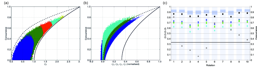
Figure 4: $(a)$ Numerical simulations of two-qubit states indicate that the concurrence can be bounded from above (dashed) and below (solid) using the reference-frame independent quantity $Q_{2}$. Colours visualise the purity of the state. $(b)$ Normalised higher-order quantities depending on two-body correlations ($Q_{3}$ in dark blue, $Q_{4}$ in green, $Q_{5}$ in light blue) may allow tighter bounds on the concurrence. $(c)$ Experimental measurements of $Q_{2}$, …, $Q_{5}$ of the maximally entangled state $\left|\phi^{-}\right\rangle.$ with about $91\%$ fidelity (rotation $1$) and nine local unitary rotations of it. The thereby deduced blue-shaded measurements of the moments allow to bound the concurrence (gray-blue shaded intervals around $0.9$) which is well above the threshold of $1/3$. Figure taken from Lawson et al. [195].

As shown in Fig. 4, for a given value of $Q_{2}$, the concurrence can be bounded from both sides. As observed, only states with higher purities can achieve higher values of $Q_{2}$ as visible from the colour encoding (increasing purities from dark blue with $\mathcal{P}\leq 0.5$ over green, red and light blue to yellow with $\mathcal{P}\in[0.8,0.9]$). In a similar fashion, the concurrence of simulated two-qubit states is shown against the normalised $Q_{3}$, $Q_{4}$ and $Q_{5}$ in Fig. 4. This strongly suggests that large respective values of the latter lead to tighter bounds on the concurrence. For the experimental demonstration, Lawson et al. use a commercial spontaneous down-conversion source and perform local-unitary rotations on one of the two qubits using waveplates. As the state is assumed to be a maximally entangled $\left|\phi^{-}\right\rangle=\left(|00\rangle-|11\rangle\right)/\sqrt{2}$ state, this is formally equivalent to a rotation of both qubits and demonstrates the direct experimental accessibility of the $Q_{t}$ polynomials, see Fig. 4.

3.6 Bipartite systems of higher dimensions

Although it is not trivial to generalise the methods presented so far to higher dimensional systems, at least for two-qudit states, i.e. the case of $n=2$ with local dimension $d$ and product observables $\mathcal{M}=M_{A}\otimes M_{B}$, several entanglement criteria can be found. As in the qubit case, a basic approach aims to derive criteria based on the second moment of the distributions of correlations and a more refined approach takes higher orders into account, allowing even to certify weakly entangled states such as bound entanglement.

3.6.1 Second moments

In the qubit case with $d=2$, the moments can be easily evaluated by virtue of the concept of spherical designs discussed in Sec. 3.3. This is based on the fact that unitary transformations on qubits can be regarded as orthogonal rotations on the Bloch sphere, due to the connection between $\text{SU}(2)$ and $\text{SO}(3)$ groups. In the qudit (higher dimensional) case, on the other hand, we lack the connection since the notion of a Bloch sphere is not available. Accordingly, not all possible observables are equivalent under random unitaries. However, as long as they are traceless the second moments do not depend on the choice of observables [17, 143]. In fact, one can evaluate the second moments and turn them to the sector lengths. In the following, we denote that $\mathcal{R}_{A}^{(2)}=S_{1}^{A}$, $\mathcal{R}_{B}^{(2)}=S_{1}^{B}$, $\mathcal{R}_{A}^{(2)}+\mathcal{R}_{B}^{(2)}=S_{1}$, and $\mathcal{R}_{AB}^{(2)}=S_{2}$, where $S_{1}$ and $S_{2}$ are the sector lengths in Eq. (10).

In Ref. [17], it has been shown that any two-qudit separable state obeys

$$\mathcal{R}_{AB}^{(2)}\leq(d-1)^{2}.$$ (54)

In Ref. [143], the entanglement detection has been improved using the marginal moments $\mathcal{R}_{A}^{(2)}$ and $\mathcal{R}_{B}^{(2)}$. Any separable state obeys

$$\mathcal{R}_{AB}^{(2)}\leq d-1+(d-1)\mathcal{R}_{A}^{(2)}-\mathcal{R}_{B}^{(2)}.$$ (55)

Again, any violation implies that the state is entangled. This detection method was shown to be strictly stronger than the criterion in Eq. (54). The criterion in Eq. (55) is equivalent to the second-order Rényi entropy criterion [197] stating that any separable state obeys $H_{2}(\varrho_{A})\leq H_{2}(\varrho_{AB})$, $H_{2}(\varrho_{B})\leq H_{2}(\varrho_{AB})$, where $H_{2}(\varrho)$ was defined in Sec. 2.6. The $H_{2}(\varrho)$ has been estimated by local randomised measurements in Refs. [197, 55], where an ion-trap quantum simulator was used to perform measurements of the Rényi entropy. We note that the criterion in Eq. (55) was extended to detect the Schmidt number [198] and that higher-order Rényi entropy criteria were also presented [189, 199, 200, 149]. As a final remark, the violation of Eq. (55) does not detect a weak form of entanglement known as bound entanglement, which cannot be distilled into pure maximally entangled states [111] and may not be verified by the PPT criterion [201].

3.6.2 Fourth and higher-order moments

Several entanglement criteria, the ones based on second moments and, of course, all the ones based on PT moments from randomised measurements fail to detect bound entangled states. In this section, we explain that higher-order moments are able to detect such weakly entangled states.

Let us begin by noting again that higher-order moments $\mathcal{R}^{(t)}$ for $t>2$ from randomised measurements in high dimensions ($d>2$) depend on the choice of the observable, unlike the case of qubits or second moments in high dimensions. Ref. [143] has offered a systematic method to address this problem. The key result is that one can find observables $\mathcal{M}=M_{A}\otimes M_{B}$ such that the moments $\mathcal{R}^{(t)}$ coincide with alternative moments as uniform averages over a high-dimensional sphere, the so-called pseudo-Bloch sphere, with

$$\mathcal{S}^{(t)}=N_{d,t}\int\mathrm{d}\mathbf{u}_{a}\int\mathrm{d}\mathbf{u}_{b}\left\{\operatorname{\mathrm{tr}}[\varrho_{AB}(\mathbf{u}_{a}\cdot\mathbf{\lambda})\otimes(\mathbf{u}_{b}\cdot\mathbf{\lambda})]\right\}^{t}.$$ (56)

Here, $\mathbf{u}_{a},\mathbf{u}_{b}$ denote $(d^{2}-1)$-dimensional unit real vectors uniformly distributed over the pseudo-Bloch sphere, $\mathbf{\lambda}=(\lambda_{1},\cdots,\lambda_{d^{2}-1})$ is the vector of Gell-Mann matrices, and $N_{d,t}$ is a suitable normalisation constant. Also, the observables $M_{A}$ and $M_{B}$ are defined by a suitable choice of the eigenvalues for the coincidence between $\mathcal{R}^{(t)}$ and $\mathcal{S}^{(t)}$ [143, 144]. It is essential that the moments $\mathcal{S}^{(t)}$ are invariant not only over all local unitaries but also over all changes of local operator basis $\mathbf{\lambda}$, meaning the independence of the specific choice of observable.

In fact, the moments $\mathcal{S}^{(t)}$ for $t=2,4$ for any dimension can be evaluated analytically and are simply expressed as

$$\mathcal{S}^{(2)}=\sum_{i=1}^{d^{2}-1}\tau_{i}^{2},\qquad\mathcal{S}^{(4)}=2\sum_{i=1}^{d^{2}-1}\tau_{i}^{4}+(\mathcal{S}^{(2)})^{2},$$ (57)

where a suitable normalisation constant $N_{d,t}$ is chosen and $\tau_{i}$ are singular values of the two-body correlation matrix $T=(T_{ij})$ with $T_{ij}=\operatorname{\mathrm{tr}}[\varrho_{AB}\lambda_{i}\otimes\lambda_{j}]$ for $i,j=1,\ldots,d^{2}-1$. This results from the fact that the moments $\mathcal{S}^{(t)}$ are invariant under local orthogonal rotations of the matrix $T$. Accordingly, in a similar manner to Sec. 3.5.1, one can consider the space spanned by the moments $(\mathcal{S}^{(2)},\mathcal{S}^{(4)})$ and formulate separability criteria in this space. As a suitable constraint for this purpose, the so-called de Vicente criterion proposed in Ref. [202] was used. Any two-qudit separable state obeys $\|T\|_{\text{tr}}=\sum_{i=1}^{d^{2}-1}\tau_{i}\leq d-1$, where $\|\cdots\|_{\text{tr}}$ denotes the trace norm, invariant under orthogonal transformations. This results in the set of admissible values $(\mathcal{S}^{(2)},\mathcal{S}^{(4)})$ for separable states in any dimension $d$, which allows for the detection of various bound entangled states. This is illustrated in Fig. 5. As further generalisations, the characterisation of the Schmidt number as dimensional entanglement has been discussed using this method in Refs. [144, 203].

The above method to detect bound entanglement has been implemented experimentally for two-qutrit chessboard states [204]: $\varrho_{\text{ch}}=(1/N)\sum_{i=1}^{4}\left|V_{i}\right\rangle\!\left\langle V_{i}\right|$, which are written as a mixture of four unnormalised eigenstates $\left|V_{i}\right\rangle$. The chessboard state was created by first generating two-qubit polarisation-entangled photon pairs through a spontaneous parametric down-conversion process and subsequently transforming them to two-qutrits $\left|V_{i}\right\rangle$ via dimension-expanding local operations with motorised rotating half-wave plates and quarter-wave plates. The experimentally prepared chessboard state $\varrho_{\text{ch}}^{\text{exp}}$ has a fidelity beyond $98\%$ with the mixture between $\varrho_{\text{ch}}$ and the white noise level $p=0.129$. For this state, the second and fourth moments $(\mathcal{S}^{(2)},\mathcal{S}^{(4)})$ were computed, and its entanglement was verified in Ref. [205].

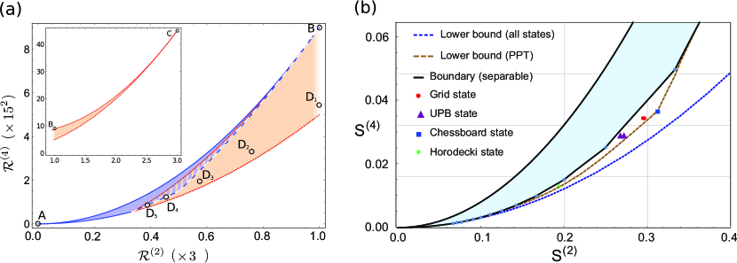
Figure 5: Left panel presents the set of Bell-diagonal states in the space spanned by the second and fourth moments $(\mathcal{R}^{(2)},\mathcal{R}^{(4)})$ with suitable normalisation of randomised measurements  [18]. Separable states are contained in the area surrounded by blue solid lines, while entangled states are outside and are contained in the area surrounded by red dotted lines. The striped region means a non-zero overlap between separable and entangled states. Labelled circles represent the maximally mixed state (A), the pure product states (B), the Bell states (C), and the reduced states of the $n$-qubit Dicke state for $n=3,\ldots,7$ with two excitations ($\text{D}_{1}$) to ($\text{D}_{5}$). Right panel shows the set of two-qutrit states in the space spanned by the second and fourth moments, denoted as $(\mathcal{S}^{(2)},\mathcal{S}^{(4)})$ in Eq. (57), with suitable normalisation of randomised measurements [143]. Separable states are contained in the light-blue area, while several bound entangled states (denoted by coloured symbols) are outside, implying that they can be detected with the method discussed in Sec. 3.6.2. Figures taken from Ketterer at al. [18] and Imai et al. [143] respectively.

3.7 Multipartite entanglement structure

The previous discussion was focused on verifying the presence of entanglement in bipartite quantum systems. In multipartite systems, the structure of entanglement can vary significantly between states culminating in genuine multipartite entanglement (GME). In this Section, we present a series of criteria for the analysis of multipartite entanglement which are all based on functions of both the full as well as the marginal second moments. We also discuss the results of a four-qubit experiment in which one of these criteria is applied to detect several types of entanglement.

3.7.1 Full separability

The detection of high-dimensional multipartite entanglement was discussed using the $k$-body sector length $S_{k}$. In Refs. [33, 206, 207, 16, 208], it has been shown that any $n$-qudit fully separable state obeys

$$S_{k}\leq\binom{n}{k}(d-1)^{k},$$ (58)

where $S_{k}$ is the $k$-body sector length. Violation of this bound implies that the state is entangled as can be easily demonstrated, for instance, in graph states. Note that this criterion can be seen as a generalisation of Eq. (54) to sector lengths between a number of observers smaller than $n$ and any dimension. One can also consider linear combinations of various sector lengths as it was shown in Ref. [209] that

$$\sum_{k=0}^{n}[(d-1)n-dk]S_{k}\geq 0$$ (59)

holds for any $n$-qudit fully separable state. This criterion is strictly stronger (detects more entangled states) than the one in Eq. (58) and can be understood as the $n$-qudit generalisation of Eq. (55).

3.7.2 $k$-separability

In order to introduce the notion of $k$-separability [118, 119], let us first consider pure states. A $n$-particle pure state is called $k$-separable if it can be written as

$$|{\psi_{k\text{-sep}}}\rangle=\left|\phi_{1}\right\rangle\otimes\left|\phi_{2}\right\rangle\otimes\cdots\otimes\left|\phi_{k}\right\rangle.$$ (60)

A mixed state is $k$-separable if it is a convex mixture of pure $k$-separable states, with different elements in the mixture possibly admitting different partitions into $k$ subsystems. For $k=n$, this notion is equivalent to the full separability. For example, the following state is $100$-qubit $12$-separable:

$$|{\psi_{100,12}}\rangle=\left|\text{GHZ}_{20}\right\rangle^{\otimes 3}\otimes\left|\text{GHZ}_{10}\right\rangle^{\otimes 2}\otimes\left|\text{GHZ}_{5}\right\rangle^{\otimes 2}\otimes\left|\text{Bell}\right\rangle^{\otimes 5}.$$ (61)

In Ref. [210], the hierarchical criteria for $k$-separability have been proposed using the full-body sector lengths $S_{n}$: any $n$-qubit $k$-separable state obeys

$$S_{n}\leq\begin{cases}3^{k-1}\;2^{n-(2k-1)},\ &\text{if \ odd}\ n,\\ 3^{k-1}\;\Big{(}2^{n-(2k-1)}+1\Big{)},\ &\text{if \ even}\ n,\end{cases}$$ (62)

for $k=2,3,\ldots,\lfloor(n-1)/2\rfloor$. A violation of the inequality for some $k$ implies that the state is at most $(k-1)$-separable. In particular, if the state violates the inequality with $k=2$, then it is verified to be genuinely $n$-partite entangled for $n>4$.

3.7.3 Tripartite entanglement

One idea to detect entanglement using second moments more efficiently is to consider linear combinations of full and marginal moments. Note that the sector lengths themselves are convex functions, but their combinations do not necessarily have to be convex. Recall that the relations between the sector lengths and the second moments are $\mathcal{R}_{A}^{(2)}+\mathcal{R}_{B}^{(2)}+\mathcal{R}_{C}^{(2)}=S_{1}$ and $\mathcal{R}_{AB}^{(2)}+\mathcal{R}_{BC}^{(2)}+\mathcal{R}_{CA}^{(2)}=S_{2}$, and $\mathcal{R}_{ABC}^{(2)}=S_{3}$, see Eq. (10). In Ref. [143], it has been shown that any fully separable three-qudit state obeys

$$S_{3}\leq d-1+\frac{2d-3}{3}S_{1}+\frac{d-3}{3}S_{2},$$ (63)

whereas any three-qudit state which is separable for any fixed bipartition obeys

$$S_{2}+S_{3}\leq\frac{d^{3}-2}{2}(1+S_{1}).$$ (64)

In the case of $d=2$, strong numerical evidence suggests that the above inequality also holds for mixtures of biseparable states with respect to different partitions [143], discussed in Eq. (23). This conjecture implies the presence of genuinely three-qubit entanglement, but its analytical proof has not yet been provided.

It is essential to note that the criteria in Eqs. (63, 64) for $d=2$ can be interpreted as the geometry of the three-qubit state space in terms of sector lengths $(S_{1},S_{2},S_{3})$ [26, 143]. In this space, both criteria were shown to be much more effective in certifying entanglement than criteria based only on the full sector length $S_{3}$. In particular, Eq. (64) can detect multipartite entanglement for mixtures of GHZ states and W states, even if the three-tangle [109] and the bipartite entanglement in the reduced subsystems vanish simultaneously [211].

3.7.4 Nonlinear functions of second moments

In Ref. [212], another criterion based on products of marginal moments was formulated. Instead of considering the factorisability of the correlation functions themselves, the factorisability of the second moments is considered with a purity-dependent bound. Namely, for two-qubit states, the inequality obeyed by all separable states reads

$${\mathcal{M}}_{2}\equiv\mathcal{R}_{AB}^{(2)}-\mathcal{R}_{A}^{(2)}\mathcal{R}_{B}^{(2)}\leq\begin{cases}(4\mathcal{P}-1)/9&\mathrm{\;for\;}\mathcal{P}<\frac{1}{2},\\ 4(1-\mathcal{P})\mathcal{P}/9&\mathrm{\;for\;}\mathcal{P}\geq\frac{1}{2},\end{cases}$$ (65)

where $\mathcal{P}=\operatorname{\mathrm{tr}}(\varrho_{AB}^{2})$ is the state’s purity, the normalisation constant for moments was chosen as $N_{n,d,t}=1$ in Eq. (26), and a product observable $\mathcal{M}=\sigma_{z}\otimes\sigma_{z}$ was used. A violation of this inequality implies the presence of entanglement between the parties. Unlike the previously presented results, this criterion is expressed as the nonlinear combination of the second moments. It is essential that this nonlinearity can enhance the detection power compared to the criterion discussed in Eq. (4). Additionally to the purity-dependent inequality for two-qubit states, inequalities for three- and four-qubit states have been obtained using numerical simulations. To indicate genuine tripartite (four-partite) entanglement, the value of ${\mathcal{M}}_{3}$ (${\mathcal{M}}_{4}$) has to overcome the bounds given by

$${\mathcal{M}}_{3} = \mathcal{R}_{ABC}^{(2)}-\mathcal{R}_{A}^{(2)}\mathcal{R}_{BC}^{(2)}-\mathcal{R}_{B}^{(2)}\mathcal{R}_{AC}^{(2)}-\mathcal{R}_{C}^{(2)}\mathcal{R}_{AB}^{(2)}\leq\tfrac{8}{27}(1-\mathcal{P})\mathcal{P},$$ (66)

$${\mathcal{M}}_{4} = \mathcal{R}^{(2)}_{ABCD}-\frac{1}{2}\sum_{M}\mathcal{R}^{(2)}_{M}\mathcal{R}^{(2)}_{\overline{M}}\leq\tfrac{8}{81}(1-\mathcal{P}^{2}),$$ (67)

where the summation is performed over all subsets of $\{ABCD\}$ except for the full and empty set, and where $\overline{M}$ denotes the set complementary of $M$. Although the simple form of the latter two expressions raises hope for a generalisation to $\mathcal{M}_{n}$, i.e. for an expression comparing the second-order moment of the distribution of the correlations of an $n$-qubit state with the products of all second-order moments of the marginals, such an expression remained missing.

This concept has been experimentally demonstrated using a pair of polarisation-entangled photons created by means of spontaneous parametric down conversion [212]. The two entangled photons are sent into two separate interferometers, making both path and polarisation degree accessible [213]. In this experiment, no knowledge about or direct control of the measurement directions is required. However, the angles of the wave plates which were required to set the measurement directions cannot be selected from a uniform distribution because this would lead to a non-uniform sampling of the local unitaries. Hence, to ensure a uniform distribution according to the Haar measure, i.e. to distribute the measurement directions following a uniform sampling of the local Bloch spheres, appropriate unitary transformations have been randomly picked to then bring the wave plates to the angles corresponding to the drawn unitary transformation.

Four different types of four-qubit states were experimentally studied: a triseparable state, a biseparable state, a GHZ state, and a linear cluster state. After applying random local transformations to each of the four qubits, projective measurements allowed to retrieve the statistics of correlation values as shown in Fig. 6.

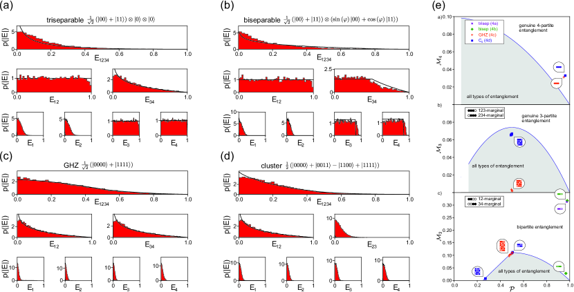
Figure 6: Panels $(a)$ to $(d)$ show histograms of experimental distributions of correlations averaged over random local measurements for a four-qubit triseparable state (a), biseparable state (b), GHZ state (c) and linear cluster state (d). Full correlations are shown alongside distributions of several of their marginal states. Here $p\left(|E|\right)$ denotes the probability distribution of modulus of the correlation value of the four-partite state (for $E_{1234}$) and some of its marginal states (for $E_{12}$, $E_{1}$, and so on). The solid lines indicate the distribution for the ideal states with infinite statistics. The rightmost panel presents the comparison of the second-order moment of the correlation distribution of an $n$-qubit state with all products of moments of marginals allowing the detection of genuine multipartite entanglement and revealing the entanglement structure of states. Figures taken from Knips et al. [212].

The shape as well as the factorisability of the particular distributions directly visualise the entanglement structure of the state. For example, for the triseparable state $\left|\textrm{Bell}\right\rangle\left|0\right\rangle\left|0\right\rangle$ the distribution of the modulus of correlation values for the marginal of the first two qubits, i.e. $E_{12}\equiv\operatorname{\mathrm{tr}}[(U_{1}^{\dagger}\sigma_{1}U_{1}\otimes U_{2}^{\dagger}\sigma_{2}U_{2}\otimes\mathbbm{1}\otimes\mathbbm{1})\varrho]$, is almost uniform and not explainable by a product of the single-qubit marginals (panels $E_{1}$ and $E_{2}$). At the same time, the other two qubits individually already show large values for $E_{3}$ and $E_{4}$, respectively, sufficient to explain the distribution $E_{34}$.

This graphical analysis illustrates how a criterion for GME allows to probe the entire entanglement structure of a state when applied to different partitions and combinations of subsystems. The rightmost panel in Fig. 6 shows the results of this structural analysis for the four experimentally prepared states, summarizing which states and marginals are violating the respective bounds. The top-most subplot ($\mathcal{M}_{4}$) indicates that both the GHZ and the linear cluster state are detected to be genuinely four-partite entangled, which is not detected for the biseparable or the triseparable state (as it should be). $\mathcal{M}_{2}$, on the other hand, shows that for the biseparable state $\left|\textrm{Bell}\right\rangle\left|\psi_{\textrm{ent}}\right\rangle$ the two-qubit marginals are still entangled, whereas the triseparable state carries entanglement solely between the first two qubits.

3.7.5 Discriminating $W$-class entanglement

In multipartite systems, the structure of entanglement becomes much richer and more complicated than in bipartite systems. In the bipartite state space, there exists an ordering structure in terms of quantum resource theories [214]. In this sense, the maximally entangled state can be defined as the entangled state that enables to create any bipartite entanglement by LOCC operations. On the other hand, in multipartite systems, such an ordering structure does not exist anymore and the notion of maximally entangled states cannot be defined uniquely. In fact, already three-qubit pure states are divided into two classes: the GHZ class and the W class. The GHZ state cannot be transformed to the W state and vice versa with LOCC operations, even if they are not required to reach the state with probability one (so-called stochastic LOCC (SLOCC) operations) [88, 215]. This distinction leads to different roles the GME states play in information processing tasks [216, 217, 218]. For four-qubit states, there is already an infinite collection of such classes, which can be grouped into nine families [219]. Therefore, in addition to entanglement detection, another interesting and important issue is to determine which class a given multipartite state belongs to.

The discrimination of $W$-class entanglement has been studied with two criteria based on the second and fourth moments of randomised measurements [220]. The first is an analytical upper bound for the second moment of a $n$-qubit $W$-class state:

$$S_{n}\leq 5-\frac{4}{n},$$ (68)

where we set $S_{n}=\mathcal{R}^{(2)}$ and the inequality is saturated by a pure $W$ state: $\left|W\right\rangle=(\left|10\cdots 0\right\rangle+\left|01\cdots 0\right\rangle+\cdots+\left|0\cdots 01\right\rangle)/\sqrt{n}$. The violation of this condition implies that a multiqubit state is detected to be outside of the W class, i.e. it cannot be obtained from the W state by SLOCC. The second criterion uses a linear combination of the second and fourth moments, with weights optimised based on the $n$-qubit $W$ state $\left|W_{n}\right\rangle$ and the biseparable state $\left|W_{n-1}\right\rangle\left|\psi\right\rangle$. Furthermore, Ref. [220] has provided the characterisation of three-qubit and four-qubit states using the second and fourth moments from an extensive numerical approach.

3.8 Finite datasets and single-setting entanglement detection

Since in experimental practice always only finite datasets are available, statistical noise additionally complicates tasks such as the certification of entanglement, which is of course also true for the scenario of randomised measurements. In this section, we present tools to analyse and quantify these statistical effects and discuss how they affect the moments of probability distributions making it possible to refine the various entanglement criteria accordingly. For more details about the field of statistical analysis on quantum systems, see Refs. [221, 222, 223, 224, 225].

3.8.1 Estimation of correlation functions

Statistical noise in the scenario of randomised measurements has two sources. The first is a result of the quantum nature of the system, for which the correlation tensor element $T_{i}$ (for fixed measurement settings collectively indexed by $i$) cannot be measured directly but has to be determined in a statistical manner via the repetition of a probabilistic measurement which can yield a set of discrete outcomes. These outcomes are distributed around the mean value $\mu_{i}=T_{i}$ with a variance of $\sigma_{i}^{2}$, which in general is a function of $T_{i}$ as well. Formally, this series of $m$ measurements can be expressed as a set of independent and identically distributed (i.i.d.) random variables $\{X_{1},X_{2},\ldots,X_{m}\}$ with the same mean and variance. In this case the sample mean $\widetilde{X}=\sum X_{i}/m$ is an unbiased and consistent estimator for $\mu_{i}$, since its expectation value is $\mathbbm{E}(\widetilde{X})=\mu_{i}$ and $\widetilde{X}$ approaches $\mu_{i}$ for increasing $m$.

The second type of statistical noise is the propagation of the fluctuation of the measured values of $T_{i}$ to any quantity calculated from them, such as for example the second moment of their distribution $\mathcal{R}^{(2)}$. Note that in this case the fluctuation of each particular $T_{i}$ additionally combines with noise due to sampling of only a finite amount of different $T_{i}$’s (different settings). For a set of $m$ measured correlation values $\{\widetilde{T}_{1},\widetilde{T}_{2},\ldots\widetilde{T}_{m}\}$ the estimator $\widetilde{\mathcal{R}}^{(2)}=\sum\widetilde{T}^{2}_{i}/m$ albeit consistent is, however, biased. Even though each particular $\widetilde{T}_{i}$ is an unbiased estimator for the corresponding $T_{i}$, the value of $\widetilde{\mathcal{R}}^{(2)}$ is systematically increased due to taking the square. Both the statistical fluctuation due to finite sample size as well as any systematic bias has to be taken into account when applying the entanglement criteria based on a bound violation, such as for example in Eq. (50). When this is properly considered, it turns out that even very limited data sets can lead to a valid conclusion about the entanglement in the system [226, 227, 228].

A common way to quantify how much the values of a general estimator $\widetilde{\theta}$ deviate from the actual parameter $\theta$ is based on the likelihood. This is generally defined as the probability of the data given some assumptions or models (e.g., the probability of tomographic data given some quantum state $\varrho$). More specifically, one can consider the probability that the an estimator takes has an observed value for a given value of the parameter, $\mathrm{Prob}(\widetilde{\theta}|\theta)$. It allows us to calculate the $p$-value, i.e. the probability that for a certain $\theta$, the estimated value of $\widetilde{\theta}$ will be sufficiently close. The usual definition is

$$\text{Prob}(|\widetilde{\theta}-\theta|\geq\delta)\leq\alpha,$$ (69)

where $\delta$ is called the error or accuracy, $\delta/\theta$ the relative error, $\alpha$ the statistical significance level, and $\gamma=1-\alpha$ the confidence level. A practical tool to estimate $p$-values are so-called concentration inequalities such as the Chebyshev inequality which for example allows to estimate the probability that the sample mean $\widetilde{X}$ from a sample of $m$ observations will be close to mean value as

$$\text{Prob}(|\widetilde{X}-\mu|\geq\delta)\leq\frac{\sigma^{2}}{m\delta^{2}}.$$ (70)

This relation allows us to estimate the minimal number of measurements $m$ to achieve a certain significance level.

3.8.2 Statistical significance and randomised measurements

To evaluate the statistical effect when applying criteria based on quantities like $\mathcal{R}^{(t)}$, it is crucial to quantify how much the estimated value can deviate from the parameter of interest, as expressed in Eq. (69). As before, we consider an experiment in which a sample of $M$ different measurement settings is chosen randomly and for each setting, measurements are performed on $K$ state copies, see Fig. 7. An unbiased estimator for the moment can be given by $\tilde{\mathcal{R}}^{(t)}=\frac{1}{M}\sum_{i=1}^{M}[\tilde{E_{t}}]_{i}$. In this expression, $\tilde{E_{t}}$ denotes the unbiased estimator of $E^{t}$ (the $t$-th power of the correlation function $E$) that is obtained from the $K$ measurements and the subscript $i$ refers to the setting.

Even in the case where $[\tilde{E_{t}}]_{i}$ cannot be assumed to be i.i.d. random variables, we can find deviation bounds such as Eq. (69) based on the variance of $\tilde{\mathcal{R}}^{(t)}$ using the Chebyshev-Cantelli inequality

$$\text{Prob}(|\tilde{\mathcal{R}}^{(t)}-\mathcal{R}^{(t)}|\geq\delta)\leq\frac{2\text{Var}(\tilde{\mathcal{R}}^{(t)})}{\text{Var}(\tilde{\mathcal{R}}^{(t)})+\delta^{2}}.$$ (71)

This leads to a minimal two-sided error bar $\delta_{\text{error}}=\sqrt{({1+\gamma})/({1-\gamma})}\sqrt{\text{Var}(\tilde{\mathcal{R}}^{(t)})},$ which guarantees the confidence level $\gamma=1-\alpha$. For instance, in the estimation of the second moment $\mathcal{R}^{(2)}$ for an $n$-qubit state with a product observable, the expression of the variance is

$$\text{Var}(\tilde{\mathcal{R}}^{(2)})=\frac{1}{M}\left[A(K)\mathcal{R}^{(4)}+B(K)\mathcal{R}^{(2)}+C(K)-(\mathcal{R}^{(2)})^{2}\right],$$ (72)

where $A(K),B(K),C(K)$ are determined through the properties of the binomial distribution, and has been derived in Ref. [210]. From this result, the total number of measurements for the precise estimation of $M_{\text{total}}=M\times K$ can be determined depending on the state under consideration and required accuracy $\delta$ and confidence level $\gamma=1-\alpha$.

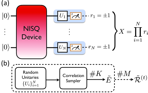
Figure 7: Characterisation of a Noisy Intermediate-Scale Quantum (NISQ) device using locally randomised measurements: (a) A measurement on $N$ qubits using random local bases defined by a set of local unitaries $\{U_{i}\}_{i=1}^{N}$, resulting in a correlation sample $X$. (b) $M$ repetitions of the measurement protocol described in (a), with each repetition using a different set of randomly sampled measurement bases. Every individual projective measurement is performed $K$ times and the overall scheme provides us with the moment estimator. Figure taken from Ketterer et al. [210].

The dependence of the second moment on the squared correlations gives rise to a systematic error that must be taken into account. Reference [212] proposes to mitigate this with the use of Bayesian methods. This requires establishing the probability $P(\tilde{T})$ with which a given value of correlations $T$, estimated after $K$ trials, occurs in the experiment. The second moment written in this language is

$$\int_{-1}^{1}\mathrm{d}T\,T^{2}\,P(T)=\int_{-1}^{1}\int_{-1}^{1}\mathrm{d}T\,\mathrm{d}\tilde{T}\,T^{2}\,P(T|\tilde{T})\,P(\tilde{T}).$$ (73)

The Bayes theorem then gives $P(T|\tilde{T})=P(\tilde{T}|T)\tilde{P}(T)/P(\tilde{T})$, where $\tilde{P}(T)$ represents the prior assumption about the unknown ideal distribution $P(T)$. In practice this prior can be chosen as estimated $P(\tilde{T})$ and the conditional probability $P(\tilde{T}|T)$ can be assumed to be a normal distribution centred at $T$ and with variance $(1-T^{2})/K$, leading to an updated estimation of the second moment $\tilde{\mathcal{R}}^{(2)}$.

3.8.3 Certification of entanglement

Table 2: Probability of bound violation for $n$-qubit GHZ state with a single random measurement per party and $p$-value of $4.6\%$. Number $K$ denotes the number of trials based on which the correlation function is estimated. The table is taken from Ref. [17].

$n$	3	4	5	6	7	8	9	10
$K=1000$	26%	44%	47%	57%	52%	48%	41%	34%
$K\rightarrow\infty$	26%	44%	48%	63%	67%	77%	80%	86%

In the case of entanglement detection with finite statistics the estimated second moment $\tilde{\mathcal{R}}^{(2)}$ may happen to be larger than $1$ also for a product state, as discussed in Ref. [16, 17]. In such a scenario, an entanglement indicator can be formulated as

$$\tilde{\mathcal{R}}^{(2)}>1+\delta\implies\textrm{likely }\left|\psi\right\rangle\textrm{ is entangled},$$ (74)

where $\varepsilon$ determines the confidence of entanglement detection. Given sufficiently big $M$ and $K$ a normal distribution a standard deviation $\Delta_{M,K}$ approximates the distribution of values of $\tilde{\mathcal{R}}^{(2)}$ for any state. A significance level of $5\%$ can be satisfied by setting $\delta=2\,\Delta_{M,K}$ in which case the probability that a separable state will yield a value within the specified bound is $95.4\%$. Hence, a measurement of a value higher than $1+2\Delta_{M,K}$ detects entanglement with a $p$-value of $4.6\%$ and confidence level of at least $95\%$.

The statistical analysis gives rise to the possibility of entanglement detection with a single randomly chosen measurement setting. Table 2 presents the probability that $n$-qubit GHZ state violates the bound $\mathcal{R}^{(2)}_{M,K}>1+\delta$, with a single randomly chosen setting ($M=1$) and $p$-value of $4.6\%$. The case of ideal quantum predictions ($K\to\infty$) is compared with $K=1000$ repetitions. For the ideal predictions, the probability violation grows with the number of qubits whereas for finite statistics the detection probability first increases but then decays.

4 Functions of states

Addressing the task of entanglement detection is vital for many quantum information applications. Nevertheless, it is not the only relevant question for quantum state analysis. One may also be interested in the functions of states, which not only can be used to verify entanglement but also to provide a description of other state features. Many quantum mechanical notions, such as the purity or PT moments explained above, are non-linear functions of the state and require in their standard definition the knowledge of the complete density matrix for their calculation, see Eq. (11) and Eq. (15) respectively. This, however, poses a challenge in experimental settings due to the exponential growth in the number of measurements required for state tomography as the number of particles increases.

Randomised measurements have emerged as a valuable approach in this domain, enabling the extraction of these quantities from experimental data with considerably fewer resources. They can be accessed through properly designed functions of probabilities over outcomes of measurements in product bases, statistical moments and other post-processing techniques. The following section provides an overview of approaches for the estimation of state functions through the use of these techniques. In addition, we will explain the notion of shadow tomography in Sec. 4.4, where randomised measurements also play a pivotal role.

4.1 Determination of invariant properties of states

A range of unitarily invariant quantities has been shown to be accessible by randomised measurements. In contrast to the methods discussed in Sec. 3, which rely mainly on the determination of statistical moments of the distribution of correlations, the approaches in this and the following subsections are based on the direct analysis of the occurring frequencies or probabilities.

4.1.1 Theoretical results

In the most general scenario, one starts with a set of (potentially nonlocal) unitary transformations $\{U\}$ and a product basis $\{|s\rangle\}=\{|s_{1}\dots s_{n}\rangle\}$ in which the measurements are performed. Without loosing generality, one can assume this to be the computational basis, as all quantities of interest in this section are invariant under a local basis change. Then, the probabilities $P_{U}(s)=\operatorname{\mathrm{tr}}(U\varrho U^{\dagger}\left|s\right\rangle\left\langle s\right|)$ of a string of results can be inferred from the experimental data. Consequently, properly designed functions of $P_{U}(s)$ averaged, e.g. over a Haar-distributed set of unitaries $\{U\}$, allow the extraction of multiple state functions.

Since the purity is invariant under any unitary transformation, it can even be accessed if the distribution is averaged under random global unitary transformations. Indeed, it was already shown early that the purity of a state can be expressed as a linear function of the ensemble average of $P_{U}(s)^{2}$ [7]. Experimentally, however, the implementation of global random unitary transformations in systems with local interactions requires significant resources [14] and a simpler protocol is desirable.

Indeed, if local unitary rotations are considered it was shown in Ref. [55, 197, 223] that the purity of $n$-qubit states can be expressed as

$$\mathcal{P}(\varrho)=2^{n}\sum_{s,s^{\prime}}(-2)^{-D[s,s^{\prime}]}\overline{P_{U}(s)P_{U^{\prime}}(s^{\prime})}.$$ (75)

Here, $U$ is a random local unitary according to the Haar measure and $\overline{\cdots}$ denotes the ensemble average over all pairs $U,U^{\prime}$ of these unitaries. Furthermore, $D[s,s^{\prime}]$ is the Hamming distance between two-bit strings, denoting the number of elements in which two $n$-tuples of measurement results differ. Note that for the qubit case, the measurements in $x,y,$ and $z$ direction form a spherical three-design, so one can replace the random unitaries by three measurements in these directions, see Sec. 2.3. Also, note that the purity $\mathcal{P}(\varrho)=\operatorname{\mathrm{tr}}{(\varrho^{2})}=\operatorname{\mathrm{tr}}(\varrho\otimes\varrho S)$ can be written as an expectation value of two copies of a state, which connects Eq. (75) to the SWAP trick in Sec. 3.3.

For two qubits, this expression can be understood in terms of the sector length. As mentioned above, we can consider local Pauli measurements, resulting in nine possible measurement combinations. Let us focus on a single term where, for definiteness, $\sigma_{z}$ is measured on both particles. In this case, the Hamming distance can take the values 0, 1 or 2. Consequently, the terms in the sum have prefactors $1,-1/2$ or $1/4$. The occurring frequencies can be derived from products of the probabilities $P(00),P(01),P(10),$ and $P(11)$ of the results of a $\sigma_{z}\otimes\sigma_{z}$ measurement. These products can also be expanded in terms of the squared expectation values $\langle\sigma_{z}\otimes\sigma_{z}\rangle^{2}$, $\langle\sigma_{z}\otimes\mathbbm{1}\rangle^{2}$, $\langle\mathbbm{1}\otimes\sigma_{z}\rangle^{2}$, and $\langle\mathbbm{1}\otimes\mathbbm{1}\rangle^{2}$. Indeed, one finds after a short calculation

$$\sum_{s,s^{\prime}}(-2)^{-D[s,s^{\prime}]}P(s)P(s^{\prime}) =1\times\left(P(00)^{2}+P(01)^{2}+P(10)^{2}+P(11)^{2}\right)$$

$$-\frac{1}{2}\left(P(00)P(01)+P(10)P(11)+\dots+P(10)P(11)\right)$$

$$+\frac{1}{4}(P(00)P(11))+P(11)P(00)+P(01)P(10)+P(10)P(01))$$

$$=\frac{9}{8}\langle\sigma_{z}\otimes\sigma_{z}\rangle^{2}+\frac{3}{8}(\langle\sigma_{z}\otimes\mathbbm{1}\rangle^{2}+\langle\mathbbm{1}\otimes\sigma_{z}\rangle^{2})+\frac{1}{8}\langle\mathbbm{1}\otimes\mathbbm{1}\rangle^{2}.$$ (76)

Averaging these terms over all nine possible measurement combinations would introduce additional prefactors occurring due to LU invariance of sector lengths, see Sec. 3.4. Then Eq. (76) contains a sum over 9 different tensor products of Pauli measurements. Each of those will recover one term of the type $\langle\sigma_{i}\otimes\sigma_{j}\rangle^{2}$, certain triples of them will give the marginal terms like $\langle\sigma_{i}\otimes\mathbbm{1}\rangle^{2}$ giving the same weight as the two-body correlation $\langle\sigma_{i}\otimes\sigma_{j}\rangle^{2}$ and all nine contribute to the term $\langle\mathbbm{1}\otimes\mathbbm{1}\rangle^{2}$. Knowing this, it is clear that the formula (76) recovers the purity, which is proportional to the total sector length in Eq. (11).

This reasoning can be further generalised to $n$-qudit systems [197, 55]. While Eq. (75) was formulated for global systems, it can be easily applied to access the information about the purity of a subsystem, by considering random unitary operations and projective measurements on the subsystem $i$ only. Therefore, the probabilities $P_{U_{i}}(s_{i})$, explicitly given as $\operatorname{\mathrm{tr}}(U_{i}\varrho_{i}U_{i}^{\dagger}\left|s_{i}\right\rangle\left\langle s_{i}\right|)$, allow to recover the reduced state’s purity. In the case of global unitary operations, the discussed approach recovers the original results presented by van Enk and Beenakker, but note that in this case the Hamming distance needs to be redefined [7].

Other interesting quantities are state overlaps and state fidelities. As shown in Ref. [224], randomised measurements allow the cross-platform estimation of

$$\mathcal{F}(\varrho_{1},\varrho_{2})=\frac{\operatorname{\mathrm{tr}}(\varrho_{1}\varrho_{2})}{\text{max}\{\mathcal{P}(\varrho_{1}),\mathcal{P}(\varrho_{2})\}},$$ (77)

with subscripts $1$ and $2$ referring to the states of two different quantum devices, labelled by $1$ and $2$. The above fidelity between mixed states was first proposed in Ref. [229] as a fidelity measure for mixed quantum states. It fulfils all of Jozsa’s axioms [230] and can be interpreted as a Hilbert-Schmidt product of the two states normalised by their maximal purity. Contrary to the widely used Uhlmann fidelity [231], it is easier to compute. Evaluation of Eq. (77) is done via the randomised measurement of cross-correlations. That means that in Eq. (75) different randomly chosen unitaries $U$ and $U^{\prime}$ are applied to the output state of the two platforms independently. Again, this can be understood as a slight generalisation of Eq. (76); it can also be understood as a version of the SWAP trick in the form of $\operatorname{\mathrm{tr}}{(\varrho_{1}\varrho_{2})}=\operatorname{\mathrm{tr}}(\varrho_{1}\otimes\varrho_{2}S)$.

In this spirit, the presented approach to randomised measurements is not limited to informational concepts only. It can also provide protocols for the measurement of many-body topological invariants (MBTIs) of symmetry-protected-topological phases. Likewise the Rényi entropy, MTBIs are non-linear functions of the reduced density matrices. The authors in Ref. [232] proposed a measurement scheme for MTBIs associated with the partial reflection, time reversal and internal symmetry [233] of one-dimensional interacting bosonic systems. Both of these quantities can be estimated using ensemble averages in a similar manner as in Eq. (75).

4.1.2 Experimental implementations

A significant amount of experimental work was invested into demonstrating the feasibility of the above discussed techniques. Starting from the result presented in Eq. (75), the second-order Rényi entropy defined in Eq. (13) was used to measure the entanglement entropy in an ion system. The measurements were performed for partitions of up to $10$ qubits of a string of $20$ qubits in a trapped-ion quantum simulator using ${}^{40}\mathrm{Ca}^{+}$ [55], see Fig. 8 for a part of the results. This experiment involved an application of $M=500$ unitary operations, generated numerically according to an algorithm given in Ref. [234], each followed by $K=150$ repetitions of measurement.

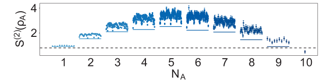
Figure 8: Experimental data for the second-order Rényi entropy measurement in bipartitions of a $10$-qubit state realised with ${}^{40}\mathrm{Ca}^{+}$ ions. The number of ions in partition $A$ has been denoted as $N_{A}$ and $N_{A}=10$ corresponds to the global state. The dashed black horizontal line corresponds to three standard deviations above the full system’s entropy ($N_{A}=10$) and solid blue lines to three standard deviations below the minimal subsystem’s entropy for a given $N_{A}<10$. The data demonstrate entanglement across all the $2^{9}-1=511$ bipartitions. The randomised protocol involved $M=500$ random unitary operations [234], each followed by $K=150$ repetitions of measurement. Figure taken from Ref. [55].

The measurement of the entropy over the time evolution of a state allows to study the dynamical properties of quantum many-body systems. A ballistic (linear) entropy growth is present for an interacting quantum system without disorder which will reach thermalisation, whereas a logarithmic entropy growth is expected for a system with strong disorder and sufficiently short-ranged interactions. The latter system will exhibit many-body localisation (MBL) [235]. Measurements of the entropy growth in Ref. [55] showed the diminishing effect of local, random disorder on the growth rate at early times compared to a system without disorder indicating localisation. Furthermore, the evolution of the second-order Rényi mutual information was detected providing another indicator of localisation due to the presence of disorder in the system.

Another quantity which is related to multipartite entanglement of many-body systems is the quantum Fisher information (QFI) [236, 237, 117, 238]. The inverse of the QFI sets a fundamental limit on the accuracy of parameter-estimation measurements and thus quantifies the potential of a quantum state in metrological applications [116]. In Ref. [239] the QFI was estimated via randomised measurements using two different platforms: a nitrogen-vacancy (NV) center spin in diamond and a superconducting four-qubit state provided by IBM Quantum Experience. For the one-qubit NV system, the dynamical evolution of the QFI was measured showing the applicability of the scheme to both pure and mixed quantum states. In the latter case, for multi-qubit states a lower bound on the QFI is set [240].

Randomised measurements also provide a powerful and experimentally feasible method to probe quantum dynamics. One example is quantum information scrambling which describes how initially localised quantum information becomes, during time evolution, increasingly nonlocal and distributed over the entire system under consideration. Scrambling can be measured via the decay of an out-of-time-order (OTO) correlation function. Randomised measurements allowed for the measurement of these OTO correlation functions in a four-qubit nuclear magnetic resonance based quantum simulator [241] and in a system of 10 trapped ions with local interactions of tunable range [242].

4.2 Estimation of higher PT moments

As explained in Sec. 2.7, bipartite entanglement of $\varrho_{AB}$ can be detected using the so-called PT moments, denoted as $p_{k}=\operatorname{\mathrm{tr}}[(\varrho_{AB}^{\Gamma_{B}})^{k}]$. The second PT moment $p_{2}$ is nothing but the state’s purity and its estimation from randomised measurements was already discussed in the previous section. Further analysis of a state, of course, involves higher-order PT moments that include essential information about the state. As an example, it was shown that they become especially useful for extracting the logarithmic negativity [54]. So the question arises how to obtain higher PT moments from randomised measurements. To address this, one needs to develop strategies of randomised measurements, such as generalisations of the SWAP trick mentioned in Sec. 4.1. In the following, we will focus particularly on the third $p_{3}$ moment, reviewing the results given in Refs. [50, 51].

Let us begin by noticing that $p_{3}$ can be rewritten using a Hermitian operator $M_{\text{neg}}$ acting on three copies of $\varrho_{AB}$,

$$p_{3}=\operatorname{\mathrm{tr}}\left[\varrho_{AB}^{\otimes 3}M_{\text{neg}}\right],\qquad M_{\text{neg}}=\frac{1}{2}\left(W_{\text{cyc}}^{A}\otimes W_{\text{inv}}^{B}+W_{\text{inv}}^{A}\otimes W_{\text{cyc}}^{B}\right),\qquad W_{\text{inv}}^{X}=(W_{\text{cyc}}^{X})^{-1}=(W_{\text{cyc}}^{X})^{T},$$ (78)

where $W_{\text{cyc}}^{X}$ is the cyclic operator with $W_{\text{cyc}}^{X}\left|s_{1},s_{2},s_{3}\right\rangle=\left|s_{2},s_{3},s_{1}\right\rangle$ acting on the subsystem $X=A,B$ of the three copies, for details see Sec. 3.3. With this expression, one can understand the operator $M_{\text{neg}}$ in the scheme of randomised measurements. First, note that the third moment $\mathcal{R}_{\mathcal{M}}^{(3)}$ defined in Eq. (26) with an observable $\mathcal{M}$ acting on the whole system $AB$ can be reformulated as

$$\mathcal{R}^{(3)}_{\mathcal{M}}(\varrho_{AB})=N_{2,d,3}\operatorname{\mathrm{tr}}\left[\varrho_{AB}^{\otimes 3}\Phi_{A}^{(3)}\otimes\Phi_{B}^{(3)}(\mathcal{M})\right].$$ (79)

Here we denoted $\Phi_{X}^{(t)}(X)=\int\mathrm{d}\mu(U_{X})\,U^{\otimes t}X^{\otimes t}(U^{\dagger})^{\otimes t}$ as the $t$-fold twirling operation on system $X=A,B$, see Sec. 3.3.3. This representation gives an alternative interpretation of the $t$-th moment $\mathcal{R}_{\mathcal{M}}^{(t)}(\varrho)$ as an expectation of a locally-twirled observable on $t$ copies of the state $\varrho$. So, the question arises how to choose the observable $\mathcal{M}$ such that the desired $M_{\text{neg}}$ is achieved by twirling, $\Phi_{A}^{(3)}\otimes\Phi_{B}^{(3)}(\mathcal{M})$.

To proceed, notice that the operator $M_{\text{neg}}$ can be also decomposed into $M_{\text{neg}}=\frac{1}{4}(M_{+}^{A}\otimes M_{+}^{B}-M_{-}^{A}\otimes M_{-}^{B}),$ where $M_{\pm}^{X}=W_{\text{cyc}}^{X}\pm W_{\text{inv}}^{X}$ for $X=A,B$. In Ref. [50], each of these terms was shown to be accessible with randomised measurements. More precisely, there exist a product observable $\mathcal{M}_{\text{P}}=\mathcal{M}_{A}\otimes\mathcal{M}_{B}$ and a non-product (Bell-basis) observable $\mathcal{M}_{\text{Bell}}$ such that

$$\Phi_{A}^{(3)}\otimes\Phi_{B}^{(3)}(\mathcal{M}_{\text{P}})=M_{+}^{A}\otimes M_{+}^{B},\qquad\Phi_{A}^{(3)}\otimes\Phi_{B}^{(3)}(\mathcal{M}_{\text{Bell}})=M_{-}^{A}\otimes M_{-}^{B}.$$ (80)

This immediately leads to the result $M_{\text{neg}}=(1/4)\Phi_{A}^{(3)}\otimes\Phi_{B}^{(3)}(\mathcal{M}_{\text{P}}-\mathcal{M}_{\text{Bell}})$, showing that the operator $M_{\text{neg}}$ can be realised by combining the product and non-product observables from randomised measurement schemes.

In a similar manner, higher-order PT moments can be evaluated as an expectation value of a permutation operator acting on $k$ copies of $\varrho_{AB}$ [51]

$$p_{k}=\operatorname{\mathrm{tr}}\left[\varrho_{AB}^{\otimes k}W_{\text{cyc}}^{A}\otimes W_{\text{inv}}^{B}\right],$$ (81)

where $W_{\text{cyc}}^{A}$ and $W_{\text{inv}}^{B}$ are $k$-copy cyclic operators $W_{\text{cyc}}^{A}\left|s_{1},\cdots,s_{k}\right\rangle=\left|s_{2},\cdots,s_{k},s_{1}\right\rangle$ and $W_{\text{inv}}^{B}\left|s_{1},\cdots,s_{k}\right\rangle=\left|s_{k},s_{1},\cdots,s_{k-1}\right\rangle$ acting on partition $A$ or $B$.

In the following, we shortly explain another way to estimate the higher moments $p_{k}$ based on tomographic methods shown in Refs. [223, 243], for more details see also Sec. 4.4 below. A key idea is to create the unbiased estimator $\hat{\varrho}_{AB}^{(r)}$ for $\varrho_{AB}$ from a data set of projective measurements results with different random unitaries $r=1,2,\ldots,M$. Based on this, one can define the unbiased estimators for the PT moments as

$$\hat{p}_{k}=\frac{1}{k!}{M\choose{k}}^{-1}\sum_{r_{1}\neq\cdots\neq r_{k}}\operatorname{\mathrm{tr}}\left[W_{\text{cyc}}^{A}\otimes W_{\text{inv}}^{B}\hat{\varrho}_{AB}^{(r_{1})}\otimes\cdots\otimes\hat{\varrho}_{AB}^{(r_{k})}\right],$$ (82)

where $r_{i}$ labels the data acquired from the measurements performed after the action of $r\,$th unitary. This results from the so-called $U$-statistics properties and the factorisation of $\varrho_{AB}^{\otimes k}$ into the products. Implementing these techniques can estimate the PT moments, therefore allowing for the certification of entanglement through $p_{k}$-PPT and the optimal $p_{k}$-OPPT criteria discussed in Sec. 2.7.

4.3 Makhlin invariants

The previous sections described the determination of the purity of states or PT moments using randomised measurements, while Sec. 3 discussed the statistical moments $\mathcal{R}^{(t)}$ as correlation-type quantities such as sector lengths. All the resulting quantities were LU invariant and from arguments as in Eqs. (76) and (78) one can infer that arbitrary LU invariants can be measured with randomized measurements. So, the question arises how randomised measurements can be used to completely characterise the LU orbit of a quantum state. For two qubits, there is indeed a complete set of LU invariants, the so-called Makhlin invariants and here we explain how they can be determined with randomised measurements [142].

Let us begin by recalling that two quantum states $\varrho$ and $\sigma$ are called LU equivalent if and only if one can be transformed into the other by local unitary operation $U_{A}\otimes U_{B}$, that is, $\varrho=(U_{A}\otimes U_{B})\sigma(U_{A}^{\dagger}\otimes U_{B}^{\dagger})$. Clearly, two LU equivalent states have the same values of quantities invariant under LU operations. Conversely, one may ask whether there is a (finite) set of invariants, such that two states are LU equivalent if they have the same values for these invariants. In two-qubit systems, this question was answered by Makhlin [41]. It has been shown that two two-qubit states $\varrho$ and $\sigma$ are LU equivalent if and only if they have equal values of all $18$ LU invariants $I_{1},\ldots,I_{18}$, nowadays called the Makhlin invariants.

Using the notation in Eq. (8) from Sec. 2, the first three invariants are given by:

$$I_{1}=\det(T),\ \ \ I_{2}=\operatorname{\mathrm{tr}}(TT^{\top}),\ \ \ I_{3}=\operatorname{\mathrm{tr}}(TT^{\top}TT^{\top}).$$ (83)

These three invariants are already sufficient to compute a potential violation of the CHSH quantity, given by $S(\varrho)=2\sqrt{\lambda_{1}+\lambda_{2}}$, as discussed in Sec. 2.8. This is because the two largest eigenvalues $\lambda_{1}$ and $\lambda_{2}$ of the matrix $TT^{\top}$ can be obtained from its characteristic polynomial and therefore can be computed from $I_{1}$, $I_{2}$, and $I_{3}$.

Reference [142] has demonstrated that these invariants can be accessed from the moments $\mathcal{R}^{(t)}$ from randomised measurements, providing a tool to certify Bell nonlocality in a reference-frame-independent manner. Using a similar approach, one can derive a lower bound on the teleportation fidelity of the state [244, 142, 245].

It is worth noting that $I_{2}$ and $I_{3}$ are also invariant under the partial transposition of a state, while $I_{1}$ flips the sign. This distinction corresponds to the fact that $I_{2}$ and $I_{3}$ can be obtained using randomised measurements with the product observable $\mathcal{M}_{\text{P}}=\sigma_{z}\otimes\sigma_{z}$, whereas $I_{1}$ comes from the non-product observable $\mathcal{M}_{\text{NP}}=\sum_{i=x,y,z}\sigma_{i}\otimes\sigma_{i}$. In addition, the invariant $I_{14}=\operatorname{\mathrm{tr}}(H_{a}TH_{b}^{\top}T^{\top})$ also flips the sign under partial transposition, where $(H_{x})_{ij}=\sum_{k=x,y,z}\epsilon_{ijk}x_{k}$ represents the elements of a skew-symmetric matrix constructed from the Bloch vectors of the reduced states $x_{k}=a_{k},b_{k}$ and the Levi-Civita symbol $\epsilon_{ijk}$. Also, the invariant $I_{14}$ was shown to be obtained from combinations of different non-product observables: $\mathcal{M}_{\text{NP}}^{\pm}=\mathbbm{1}\otimes\sigma_{x}+\sigma_{x}\otimes\mathbbm{1}+\sigma_{y}\otimes\sigma_{z}\pm\sigma_{z}\otimes\sigma_{y}$. The LU invariants $I_{1}$ and $I_{14}$ are sensitive to partial transposition and then play a crucial role in implementing the PPT criterion in randomised measurements, as explained in Sec. 3.5.2.

Let us shortly explain the experimental scheme to obtain the LU invariants $I_{1}$, $I_{2}$, and $I_{3}$ from the moments $\mathcal{R}^{(t)}$ of randomised measurements [142]. The creation of two-qubit states was implemented by polarisation-entangled photon pairs from an entangled photon source (EPS). This generates signal and idler photon pairs via four-wave mixing in a dispersion-shifted fiber (DFS). In the detector station (DS), each photon is detected with an efficiency of about $20\,\%$ and dark count probabilities about $4\times 10^{-5}$ per gate.

The experimental generation of random unitaries has been accomplished using polarisation scramblers (SCR) as depicted in Fig. 9. These can rapidly change the Stokes vector in the Bloch sphere and create random polarisation rotations. Clearly, it is necessary to check that a set of unitaries generated in this way is really Haar random. Here, it is sufficient to show that the used random unitaries form a unitary $t$-design with an appropriate order $t$, depending on the degrees of the polynomial used in the evaluation. One can confirm the degree of the Haar randomness for a set of unitaries by computing the frame potential, discussed in Sec. 3.3. Recall that unitary $t$-designs only achieve the minimal value of the frame potential and can correspond to the $t$-th moments $\mathcal{R}^{(t)}$ from randomised measurements. Then, to determine the LU invariants $I_{1}$, $I_{2}$, and $I_{3}$, one has to evaluate the frame potential for a finite set of unitaries drawn order up to four and compare it with the minimal value.

Finally, the LU invariants $I_{1},I_{2},I_{3}$ were measured using their unbiased estimators $\tilde{I}_{1},\tilde{I}_{2},\tilde{I}_{3}$ from the experimental data of the set of unitaries generated, and their statistical behaviour is illustrated in Fig. 9. This analysis aimed to certify Bell’s nonlocality and assess the usefulness of quantum teleportation.

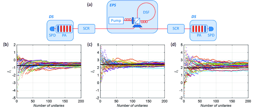
Figure 9: Panel $(a)$ shows a schematic experimental setup. The source of two-qubit entangled states (EPS) sends a signal and idler photon pairs via four-wave mixing in a dispersion-shifted fibre (DFS) to the detection station (DS). Before the measurement, random unitaries using polarisation scramblers (SCR) involving random polarisation state rotations were applied to the state. Panels $(b),(c)$ and $(d)$ present the experimental data for unbiased estimators of Mahklin $I_{1},I_{2}$ and $I_{3}$ LU invariants, respectively, plotted as a function of the number of applied unitaries. Figure taken from Ref. [142].

4.4 Randomised measurements and shadow tomography

Let us finally explain how randomised measurements can be used to obtain information about a quantum state in the framework of shadow tomography. Generally, quantum state tomography refers to the task of determining the entire density matrix from measurement data [246, 247, 248]. As the number of free parameters in the density matrix scales exponentially with the number of particles, this becomes in practice unfeasible already for a modest number of qubits.

Several methods have been suggested to circumvent the scaling problem. This includes matrix-product-state tomography [249] and compressed sensing [250], which work well if the state under scrutiny obeys certain constraints, e.g.  it has a high purity. Another example is permutationally invariant tomography [251, 252], where relevant subspaces of the entire Hilbert space are probed. Shadow tomography, proposed theoretically in Ref. [253] and suggested as a practical procedure in Ref. [243], is also a scheme to reduce the experimental effort, but here the idea is to redefine the task of tomography in a meaningful way.

In standard tomography, one determines a density matrix $\varrho$, and this is typically used for predicting the expectation values of observables that were not measured. Shadow tomography can be understood as a method to predict future measurements with high probability as good as possible [253, 243]. In a first data collection phase, measurements are carried out and for each result an (unbiased) estimator of the quantum state is recorded. The collection of all these estimators is called the classical shadow of $\varrho$ and, importantly, storing these data can be achieved with a moderate effort. As the name suggests, this task does not aim to recover the full density matrix $\varrho$, but only the shadow that $\varrho$ casts on the measurements. In the second phase, called the prediction phase, the classical shadow is used to predict other observables that were not measured in the data collection phase. Two questions are relevant: First, how does one obtain estimators for the quantum state from a single measurement result? Second, how to choose the measurements in the data collection phase in order to predict many other measurements later with high accuracy?

Let us elaborate on these points explicitly, following the description of Ref. [254]. Assume that some generalised measurement (or positive operator-valued measure, POVM) is carried out on a quantum state defined by the density matrix $\varrho$. This measurement consists of a collection of effects $E=\{E_{i}\}$ which are positive ($E_{i}\geq 0$) and normalised ($\sum_{i}E_{i}=\mathbbm{1}$) and the probabilities for the outcomes are given by $p_{i}=\operatorname{\mathrm{tr}}(\varrho E_{i}).$ This POVM defines a map from the space of density matrices to the probability distributions via

$$\Phi_{E}(\varrho)=\{\operatorname{\mathrm{tr}}(\varrho E_{i})\},$$ (84)

and the adjoint $\Phi_{E}^{\dagger}$ maps probability distributions to operators. In general, one can ask how to infer from an observed probability distribution the state $\varrho.$ Performing a single measurement of the POVM leads to a single outcome $i$, so that the distribution over the outcome probabilities $q_{i}$ corresponds to a $\delta$-type probability distribution with $\{q_{i}\}=\delta_{ik}$. The problem of how to assign an estimator to such a single-point distribution is indeed known and solved in the fields of data science and machine learning [255]. The least square estimator is the so-called shadow estimator $\chi$ and is as a map given by:

$$\chi=(\Phi_{E}^{\dagger}\Phi_{E})^{-1}\Phi_{E}^{\dagger}.$$ (85)

To assure the existence of the inverse of $C_{E}=\Phi_{E}^{\dagger}\Phi_{E}$, it is assumed that the POVM is informationally complete, that is, the state $\varrho$ can be reconstructed from the full set of probabilities $p_{i}$. With the given definition of $C_{E}$ one also directly finds that $C_{E}(\varrho)=\sum_{k}\operatorname{\mathrm{tr}}(\varrho E_{k})E_{k}$. Then, for the $\delta$-type distribution $\{q_{i}\}=\delta_{ik}$ we have that $\Phi_{E}^{\dagger}(\{q_{i}\})=E_{k}$, leading to the estimate of $\varrho$ from a single data point,

$$\hat{\varrho}_{k}=C_{E}^{-1}(E_{k}).$$ (86)

This estimator, however, does not need to be a proper quantum state; especially, $\hat{\varrho}_{k}$ may have negative eigenvalues.

So far, the discussion was general and the POVM $E$ was not specified. The key point is now that randomised measurements can be viewed as such a POVM. If one measures randomly one of the three Pauli matrices $\sigma_{x}$, $\sigma_{y}$, or $\sigma_{z}$ on a single qubit, this can be seen as a six-outcome POVM with the effects $\{\left|x^{\pm}\right\rangle\left\langle x^{\pm}\right|/3,\left|y^{\pm}\right\rangle\left\langle y^{\pm}\right|/3,\left|z^{\pm}\right\rangle\left\langle z^{\pm}\right|/3\}$. For these effects, one can directly calculate that the shadow estimator for outcome $k\pm$ is given by

$$\hat{\varrho}_{k}=3|{k^{\pm}}\rangle\langle{k^{\pm}}|-\mathbbm{1}.$$ (87)

This is not a positive semidefinite density matrix, but this does not affect it usefulness for predicting future measurements. If random Pauli measurements are carried out on $n$ qubits, the global POVM has $6^{n}$ outcomes. Most importantly, the shadow estimator is the tensor product of the single-qubit estimators as in Eq. (87). This product structure allows to store the multi-qubit shadow efficiently.

Let us now discuss the error of this procedure, if one wishes to estimate an arbitrary observable $X$ from the collection of shadows $\{\hat{\varrho}_{k_{\ell}}\}$, where $\ell=1,\dots,M$ denotes the number of measurements. First, the mean value $(1/M)\sum_{\ell}\operatorname{\mathrm{tr}}(X\hat{\varrho}_{k_{\ell}})$ converges to $\langle X\rangle=\operatorname{\mathrm{tr}}(X\varrho)$. The precision of the estimation is quantified by the variance in a single experiment, $\mathrm{Var}[\operatorname{\mathrm{tr}}(X\hat{\varrho})]=\sum_{k}\operatorname{\mathrm{tr}}(X\hat{\varrho}_{k})^{2}\operatorname{\mathrm{tr}}(\varrho E_{k})-\langle X\rangle^{2}$, which is upper bounded by the shadow norm

$$\|X\|^{2}_{E}:=\|\sum_{k}\operatorname{\mathrm{tr}}(X\hat{\varrho}_{k})^{2}E_{k}\|_{\rm op},$$ (88)

where $\|\dots\|_{\rm op}$ denotes the largest eigenvalue of an operator. Given a set $\mathcal{X}$ of observables that one wishes to predict, the quality of a shadow tomography scheme can be quantified by $\kappa^{2}_{E}=\max\{\|X\|^{2}_{E},X\in\mathcal{X}\}$. Clearly, this depends on the set $\mathcal{X}$ and the POVM $E$ chosen. Here, it turns out that the random choice of three Paulis per qubit is often the optimal choice of the POVM [254].

Finally, it is also worth noting that shadow tomography with local randomised Pauli measurements is a well suited tool for estimating observables $X$ which act on few qubits only. If $X$ acts on $L$ qubits, then it is determined by the mean values of $3^{L}$ tensor products of Paulis. In a shadow tomography scheme with $M$ randomised settings, each of these settings has, on average, been measured $M/3^{L}$ times. This provides sufficient information if $M$ is large enough, but note that the required $M$ does not depend on the number $n$ of particles. This idea can be translated to rigorous statistical statements for local observables, see Ref. [243] for details.

The scheme proposed in Ref. [243] was implemented experimentally using four-qubit GHZ states encoded with polarisation-entangled photons [256]. Three schemes with uniform, biased and derandomised classical shadows were compared to conventional ones that sequentially measure each state function using importance sampling or observable grouping, where the derandomised classical shadow method was shown to outperform other advanced measurement schemes. For other experimental implementations see Refs. [257, 258, 259].

5 Non-local correlations

In Sec. 2.8 we introduced the notion of non-local correlations and the framework of Bell-type inequalities to test them. In general, correlations not only depend on the quantum state under consideration, but also on the choice of measurements. As already discussed in the simple example of the CHSH inequality (18), in order to achieve maximal violation, the measurement settings must be chosen carefully. This requires great care in the preparation of the experiment. In the case of multi-observer Bell tests, where the efficiency of the experimental setup is much more challenging to maintain, the situation becomes even more complicated.

In this chapter, we outline how nevertheless it is possible to study quantum correlations also with randomly selected measurements. In general, to verify the presence of correlations that violate a Bell inequality (and its extensions to multipartite scenarios), it is necessary to measure several combinations of local measurement settings across the relevant parties for an entangled state. For example, let us consider the case of the CHSH inequality in a randomised measurement scenario. To measure the first expectation value $E(\mathbf{u}_{1},\mathbf{u}_{2})$, the first observer measures in the randomly chosen setting $\mathbf{u}_{1}$, while the second observer uses the randomly chosen setting $\mathbf{u}_{2}$. For the second expectation value, the second observer can switch to the randomly selected setting $\mathbf{u}^{\prime}_{2}$, while the first observer remains at setting $\mathbf{u}_{1}$. It becomes clear that for the third expectation value the second observer now has to return to the previously employed setting $\mathbf{u}_{2}$ in order to measure it jointly with a new setting of the first observer. Therefore, in all such experiments it is necessary to be able to revisit previously employed settings. Note that in typical implementations of so-called “loophole-free” Bell tests which exclude Bell-local models as possible explanations of quantum phenomena, it is additionally necessary to switch between the local settings on a shot-to-shot basis without predetermining the subsequent setting.

The type of randomness which can be present when trying to violate a Bell-type inequality, thus, cannot consist of a fluctuating noise or a total lack of control over the settings. Rather either random but fixed rotations between the reference frames of different observers (often denoted in the literature as “misaligned devices”) or even fixed, random rotations when choosing different settings within each local frame (denoted as “uncalibrated devices”) are suitable. These random rotations need to stay fixed on the timescale of data acquisition for at least one run of the respective experiment. The only exception to this is the average correlation 5.5 which is based on the first moment of the distribution of correlation functions and is thus compatible with full randomness, as in the criteria of Secs. 3 and 4.

5.1 Probability of violation

In general, when measurement settings are chosen randomly, the violation of Bell-type inequalities such as the CHSH inequality is no longer assured, even for a highly entangled state. Thus, a natural way to quantify the strength of quantum correlations in a particular system is to ask what is the probability of violation of any CHSH inequality if observers choose observables at random without caring about the precise determination of the optimal measurement settings. Such a probability (also called the “volume of nonlocality” [260] or “nonlocal fraction” [261, 262]) can be expressed by

$$\mathcal{P}_{V}^{\rm CHSH}=\int_{\Omega}\mathrm{d}\Omega\,f_{\rm CHSH}(\Omega),$$ (89)

where the integration is over all parameters that define the observable (local measurement settings) and $f_{\rm CHSH}=1$ for settings that violate any of the CHSH inequalities and $f_{\rm CHSH}=0$ otherwise. Apart from CHSH inequalities, the probability of violation $\mathcal{P}_{V}^{I}$ can of course also be formulated for any other family of Bell-type inequalities $I$. While in general the probability of violation depends on the choice of measure $\mathrm{d}\Omega$, the Haar-measure emerges as a natural choice, since in this case the probability of violation becomes invariant under local unitary rotations applied to the state [260].

In Ref. [3] the probability of violation of the CHSH inequality by the Bell state $|{\phi^{+}}\rangle=(|00\rangle+|11\rangle)/\sqrt{2}$ was derived analytically as $\mathcal{P}_{V}^{\rm CHSH}=2(\pi-3)\approx 28.32\%$. Furthermore, also in Ref. [3], the probabilities of violation for complete sets of MABK [263, 264, 265] and WWWŻB [266, 267, 80] inequalities by the $n$-particle GHZ state have been determined numerically. The violation increases with the number of particles but seems to converge asymptotically (for large $n$) to a value strictly below unity.

5.2 Strength of non-locality

The non-locality of a state $\varrho$ can not only be quantified via the probability of violation but also through the strength of non-locality $\mathcal{S}$ [268]. This quantity is based on testing how robust the correlations are under the addition of white noise. The strength is obtained by considering the noisy state $\tilde{\varrho}$ parameterized by the noise parameter $v$, so-called visibility, with

$$\tilde{\varrho}(v)=v\varrho+(1-v)\frac{1}{d^{n}}\mathbbm{1}$$ (90)

and finding the critical visibility $v=v_{\mathrm{crit}}$ below which no inequality is violated for a given set of measurement settings. The value $v_{\mathrm{crit}}$ provides the strength of non-locality via $\mathcal{S}=1-v_{\mathrm{crit}}$. The critical visibility minimized over measurements is denoted as $v_{\mathrm{crit}}^{\mathrm{min}}$ and corresponds to the maximal strength of non-locality $\mathcal{S}^{\mathrm{max}}$. For values below $v_{\mathrm{crit}}^{\mathrm{min}}$ the probability of violation reduces to $0$.

The strength of non-locality $\mathcal{S}$, does not provide complete information about the non-local properties of the state, primarily as it only quantifies for which $v$ the probability of violation $\mathcal{P}_{V}$ reduces to $0$ and not how $\mathcal{P}_{V}$ depends on variations in $v$. This information is captured, at least partially, via the average strength of non-locality $\bar{{\mathcal{S}}}$, given as the expectation value

$$\bar{{\mathcal{S}}}=\int_{0}^{\mathcal{S}^{max}}\mathcal{S}g(\mathcal{S})\mathrm{d}\mathcal{S},$$ (91)

where $g(\mathcal{S})$ is the probability density over values of $\mathcal{S}$ when choosing measurement directions according to $\mathrm{d}\Omega$, normalized such that $\int_{0}^{\mathcal{S}^{max}}g(S)d\mathcal{S}=1$. Examples of $g(\mathcal{S})$ are presented in Ref. [268]. As the number of settings per party tends to infinity, $\mathcal{S}$ becomes more and more independent of the choice of measurement directions $\Omega$ and $g(\mathcal{S})\to\delta(\mathcal{S}^{max}-\mathcal{S})$ [268]. In this case $\bar{\mathcal{S}}$ and $\mathcal{S}_{\mathrm{max}}$ become equivalent.

It is also possible to define a similar quantifier for states, the so-called “trace-weighted nonlocality strength” [269], which is based on the trace distance of Bell correlations [270] instead of the strength of non-locality of Bell correlations. Notably, just as the probability of violation, both strengths are invariant under LU. Furthermore, it can be shown that both are strictly positive for all pure entangled states in a setup with at least two binary-outcome measurements per party. The proof is based on the fact that any pure multipartite entangled state violates some two-setting two-outcome Bell inequality [271, 272].

5.3 Generalized Bell-type inequalities

The Bell scenario can be generalised to a larger number of observers $n$, measurement settings $m$, and a larger dimension of the local Hilbert space $d$. There are many examples of Bell-type inequalities for many different experimental situations [64]. However, full sets of tight Bell inequalities (Bell-Pitovsky polytopes) are known only in a few cases [65]. Moreover, the analytical determination of probabilities of violation for other states and other Bell inequalities is challenging due to the nature of the integral in Eq. (89).

A numerical method based on linear programming can, however, successfully address this problem. It is known (see, e.g. Ref. [67]) that there exists a Bell-local explanation of correlations if and only if there exists a joint probability distribution $p_{\mathrm{BL}}$ over the results of all settings for all observers, from which the experimental probabilities can be predicted via marginalisation. Thus, for a given set of measurement settings the numerical search for this probability distribution, under the constraint that it generates the experimental correlations, is equivalent to testing all possible Bell-type inequalities for these particular observables. If such a distribution can be found, it implies that the correlations are classical and thus no inequality can be violated [273]. Conversely, if the joint distribution cannot be found, the correlations are shown to be Bell non-local. In the numerical computations, this is of course true up to the numerical precision. Note that this method does neither yield nor require knowledge of the exact form of Bell-type inequalities for a given experimental situation (which are often unknown), but nevertheless effectively allows to test all of the conceivable inequalities.

By sampling the measurement settings with sufficient statistics according to the measure $\mathrm{d}\Omega$, the numerical method allows approximating the unconditioned $\mathcal{P}_{V}$, which contrary to $\mathcal{P}^{I}_{V}$ is independent of the choice of a specific family of Bell-type inequalities $I$. At the same time, the method is also extremely well suited to determine and maximise the strength of non-locality $\mathcal{S}^{\mathrm{max}}$. This numerical approach was used for the first time to the GHZ states and two measurement settings in Ref. [3] and comprehensively for various qubit and qutrit states and multiple measurement settings in Ref. [274]. It can be straightforwardly generalised to a larger number of particles, measurement settings, and sub-system dimensions, see, e.g. Ref. [275].

While the computational approach is equivalent to testing all possible Bell inequalities, it should be noted that already a single family of inequalities is sufficient to detect non-locality in most cases [268]. This optimal family with $\mathcal{P}^{\mathrm{opt}}_{V}$ is obtained by extending the CHSH inequality to more observers and settings, e.g. via a lifting procedure [276]. It turns out that for sufficiently many parties and settings $\mathcal{P}_{V}\approx\mathcal{P}^{\mathrm{opt}}_{V}$, as for example already for the three-qubit W state, $\mathcal{P}_{V}=54.893\%$, while $\mathcal{P}^{\mathrm{opt}}_{V}=50.858\%$.

5.4 Properties of the probability of violation

In the following, we briefly present the most important properties of the probability of violation and the notion of typicality of non-locality.

Dependence on number of measurement settings.—It was shown in Ref. [274] that the probability of violation increases rapidly with the number of measurement settings per party. For the GHZ state, already for two parties and five settings, $\mathcal{P}_{V}$ is close to $100\%$. This fact can be explained in two ways. Firstly, from a statistical point of view, as the number of settings increases, so does the chance of finding suitable pairs of settings. Secondly, new inequalities emerge involving all the additional measurement settings. Additionally, in Ref. [260] it is shown in general that for any pure bipartite entangled state, the probability of violation tends to unity when the number of measurement settings tends to infinity.

Multiplicativity of probability of violation.—The probability of violation is not additive, but rather multiplicative [274], in the sense that the probability $\mathcal{P}_{\mathrm{BL}}=1-\mathcal{P}_{V}$ to choose settings allowing a Bell-local explanation is multiplicative over subsystems with

$$\mathcal{P}_{\mathrm{BL}}(\varrho_{1}\otimes\varrho_{2})=\mathcal{P}_{\mathrm{BL}}(\varrho_{1})\,\mathcal{P}_{\mathrm{BL}}(\varrho_{2}).$$ (92)

This immediately hints at the increase of $\mathcal{P}_{V}$ with system size. Consider for example a product of $n$ two-qubit GHZ states ${\mathrm{GHZ}_{2}}^{\otimes n}$. Using the result $\mathcal{P}_{V}\left(\mathrm{GHZ}_{2}\right)=2(\pi-3)$ obtained above, the probability of violation becomes

$$\mathcal{P}_{V}\left({{\rm GHZ_{2}}^{\otimes n}}\right)=1-\mathcal{P}_{\mathrm{BL}}\left({{\rm GHZ_{2}}^{\otimes n}}\right)=1-\left(\mathcal{P}_{\mathrm{BL}}\left({\rm GHZ_{2}}\right)\right)^{n}=1-(7-2\pi)^{n},$$ (93)

which converges to unity for large $n$.

Maximal probability of violation.—It was shown that the $n$-particle GHZ state maximises the probability of violation for a special set of two-outcome inequalities containing only full $n$-particle correlation functions when $n$ is even [260]. More generally, if we are not restricted to any particular type of inequality and consider the full set of possible two-setting Bell inequalities (in practice only realisable via the numerical method discussed in Sec. 5.3) it turns out that the GHZ states do not exhibit the highest $\mathcal{P}_{V}$. Note that due to the numerical nature of the considerations, it is difficult to explicitly find the state which maximises $\mathcal{P}_{V}$.

Maximal non-locality and maximal entanglement.— One commonly used measure of non-locality, namely the robustness to white noise, was already introduced in Eq. (5.2). However, it has many disadvantages. One flagship example is the discrepancy between the maximal violation of the two-setting $d$-outcome CGLMP inequality [277] and its violation by the $d\times d$ maximally entangled state. It turns out that some asymmetric states tolerate a greater admixture of white noise while remaining non-local than the maximally entangled states. For the probability of violation, however, the value is maximised by the maximally entangled states and the anomaly disappears at least for $d\leq 10$ [278]. In addition, it is proven in Ref. [260] that for two qubits in a pure state the probability of violation for bipartite full-correlation Bell inequalities is an entanglement monotone.

Witness for genuine multipartite entanglement.—The probability of violation can also serve as a witness of genuine multipartite entanglement [102]. For example, for $n=3$ and two settings per party, $\mathcal{P}_{V}>2(\pi-3)$ certifies that the state is truly multipartite entangled [274]. For a larger number of particles and a larger number of settings, similar criteria can also be formulated. However, so far they are only based on numerics, see, e.g. Ref. [279].

Typicality of non-locality.—The notion of probability of violation also allows to address the question how typical non-locality is not only under variation of observables but also of states. In Ref. [274], it was shown that the typical $n$-qubit states present in many quantum information problems for $n\geq 5$ exhibit Bell non-local correlations for almost any choice of observables ($\mathcal{P}_{V}>99.99\%$). In Ref. [268], through a sampling of the whole state space of pure states it was demonstrated that for a random pure state the probability of violation strongly increases with the number of qubits and already for $N\geq 6$ it is greater than $99.99\%$.

5.5 Average correlation

An alternative to considering the probability of violation $\mathcal{P}_{V}$ has been proposed in Ref. [280]. It builds on the intuition that for example the CHSH inequality is violated if the correlations $E(\mathbf{u}_{a},\mathbf{u}_{b})$ are sufficiently high for at least two pairs of different settings. Thus, instead of testing any particular Bell-type inequality, the average correlation $\Sigma$ is calculated with

$$\Sigma=\int_{\Omega}\mathrm{d}\Omega\;|E(\mathbf{u}_{a},\mathbf{u}_{b})|,$$ (94)

i.e. it corresponds to the first moment of the modulus of the correlation function. In Ref. [280], it is conjectured and confirmed via numerical simulation that for bipartite systems $\Sigma>\sqrt{2}/4$ implies Bell non-locality and $\Sigma<1/4$ excludes it, i.e. a state with $\Sigma<1/4$ cannot violate any CHSH inequality. Compared to the testing of Bell inequalities this method has the advantage that it can be applied even in scenarios with fluctuating randomness where previous settings cannot be revisited.

5.6 Genuine multipartite non-locality (GMNL)

The notion of Bell-locality readily extends from two to an arbitrary number of parties. In a Bell-local scenario, there are only classical correlations between any of the parties and it is not possible to violate any Bell-type inequality for any partition of the system. The set of such multipartite Bell-local correlations is commonly denoted by $\mathcal{L}$. Just as with the concept of genuine multipartite entanglement, however, the notion of Bell-nonlocality can be refined to genuine multipartite non-locality (GMNL). It allows to distinguish cases where there are only some Bell non-local correlations in the system, from cases where all parties share suitable correlations.

Starting from the bi-partite definition, there are several options how to define GMNL, the first of which was proposed by Svetlichny [281]. In a straightforward formal analogy to the definition of Bell locality, it defines non-GMNL tripartite correlations as those which admit the decomposition

$$P(a,b,c|x,y,z)=\sum_{\lambda}q_{\lambda}P(a,b|x,y,\lambda)P(c|z,\lambda)+\sum_{\mu}q_{\mu}P(a,c|x,z,\mu)P(b|y,\mu)+\sum_{\nu}q_{\nu}P(b,c|y,z,\nu)P(a|x,\nu),$$ (95)

where $\lambda,\mu,\nu$ are shared parameters used to correlate measurement outcomes, the outcome of Alice when she chooses setting $x$ is denoted by $a$ and similarly pairs $y$, $b$ and $z$, $c$ denote the settings and outcomes of Bob and Charlie. Note that in each term the statistics of measurement results of one party conditionally factors out from the statistics of the other parties. In general, for $n$ observers, the set of these correlations is denoted by $\mathcal{S}_{2}$, where the subscript indicates factorisability into at least two parts. As pointed out in [282, 283] this definition is rather strict since no additional assumptions are made about the joint probability distributions such as $P(ab|xy\lambda)$. In particular they can correspond to signalling correlations, which allow for superluminal communication between parties. Note that the signalling is only a formal consequence of the decomposition since $P(abc|xyz)$ of course does not contain any signalling. This potentially unphysical nature of the decomposition motivates a different definition of non-GMNL correlations [282, 283], namely those that can be decomposed as Eq. (95), but with the additional requirement that all elements of the decomposition need to remain non-signalling, i.e. physical. The corresponding set of non-GMNL correlations is denoted as $\mathcal{NS}_{2}$. For any $n\geq 3$, this condition is strictly stronger than just requiring non Bell-local correlations, and strictly weaker than Svetlichny’s definition and therefore gives rise to the following strict inclusions $\mathcal{L}\subsetneq\mathcal{NS}_{2}\subsetneq\mathcal{S}_{2}$.

Based on these definitions, it is now straightforward to define the probability of violation $\mathcal{P}_{V}$, just as in the case of standard multipartite non-locality, as

$$\mathcal{P}_{V}(\varrho,S)=\int f(\varrho,\Omega)\leavevmode\nobreak\ \mathrm{d}\Omega,$$ (96)

where

$$f(\varrho,\Omega)=\begin{cases}1,&\text{if settings lead to correlations outside the set $S$, }\\ 0,&\text{otherwise.}\end{cases}$$ (97)

The case of $S=\mathcal{L}$ corresponds to the discussion above and $S=\mathcal{NS}_{2}$ as well as $S=\mathcal{S}_{2}$ correspond to the probability of violation given the alternative definitions of GMNL, respectively. Note that just as in the standard case, for each definition of GMNL either specific families $I$ of inequalities can be distinguished or a general probability for any type of inequality can be considered. A numerical study of these probabilities has been performed for specific inequalities $I$ in [261, 284]. For each setup (defined by the multipartite state $\varrho$, the number of settings per party $m$, and the set $\mathcal{S}$), we can single out a dominant inequality $I$ that gives the best lower bound value of $\mathcal{P}_{V}$.

Table 3: Numerically obtained probability of violation $\mathcal{P}_{V}$ for any Bell inequality and $\mathcal{P}_{V}^{I}$ for a given inequality $I$ (in $\%$) for different multipartite non-locality scenarios (denoted by $\mathcal{L}$, $\mathcal{NS}_{2}$ and $\mathcal{S}_{2}$) for two settings per party ($m=2$) and the two emblematic states $\text{GHZ}_{3}$ and $\text{W}_{3}$. The numerical values are obtained in Ref. [285], except for those where a reference is given after the value.

	$\mathcal{P}_{V}(\text{GHZ}_{3})$	$\mathcal{P}_{V}^{I}(\text{GHZ}_{3})$	$\mathcal{P}_{V}(\text{W}_{3})$	$\mathcal{P}_{V}^{I}(\text{W}_{3})$
$\mathcal{L}$	74.69 [274]	70.00 [262]	54.89 [274]	50.86
$\mathcal{NS}_{2}$	11.57	10.63	3.730	3.231
$\mathcal{S}_{2}$	0.5413	0.5353	0.0085	0.0030

In Ref. [285], the probability of violation $\mathcal{P}_{V}$ was investigated for three-party GHZ and W states with increasing number of measurement settings per party for the different tripartite scenarios (for results, see Tab. 3 for $m=2$, and see Ref. [285] for $m>2$). The following conclusions about $\mathcal{P}_{V}$ can be drawn based on Tab. 3 and on additional numerical data in the tables of Refs. [262, 285]. Importantly, $\mathcal{P}_{V}$ steadily increases with the number of measurement settings $m$ [285]. In particular, the probability of violating the $\mathcal{L}$ and $\mathcal{NS}_{2}$ conditions is greater than $99.9\%$ in the respective cases $m>3$ and $m>5$, for both $\text{W}_{3}$ and $\text{GHZ}_{3}$ states. For $\mathcal{S}_{2}$, however, this percentage is much smaller, especially for the $\text{W}_{3}$ state. This trend is observed even up to $m=6$.

The numerical computations in Refs. [262, 285] also demonstrate that in each of the three discussed tripartite scenarios, one can clearly distinguish a so-called dominant inequality, i.e. a facet of the respective convex sets $\mathcal{L}$, $\mathcal{NS}_{2}$, $\mathcal{S}_{2}$. A dominant inequality defines a family of equivalent inequalities which are most often violated for a given Bell-type experiment. As we can see in Tab. 3, the estimated $\mathcal{P}_{V}^{I}$ is surprisingly close to the $\mathcal{P}_{V}$ value for almost all two-setting ($m=2$) scenarios. In fact, the same tendency is observed for larger $m$ as well [262, 285]. In particular, a very small difference between the $\mathcal{P}_{V}^{I}$ and $\mathcal{P}_{V}$ can be observed for $\mathcal{L}$ and $\mathcal{NS}_{2}$ scenarios up to $m=6$. The worst match between the two probabilites is found in the $\mathcal{S}_{2}$ scenario for the $\text{W}_{3}$ state.

5.7 Guaranteed violation for partial randomness

It was observed that partial local alignment can lead to a significant increase in the probability of violation, culminating in the guaranteed violation, i.e. cases for which $\mathcal{P}_{V}=100\%$ (apart from trivial cases when, e.g. all measurement directions are the same). Under suitable conditions, it is robust against noise and experimental deficiencies [8].

5.7.1 Locally orthogonal settings

As mentioned above, for the case of two-qubit maximally entangled state and the CHSH inequality, when observers cannot align their measurement settings (neither between them or locally) and thus choose them randomly, the probability of violation of the CHSH inequality is approximately $28.3\%$. If, however, local calibration is possible such that each party can choose two orthogonal settings the probability increases to $41.3\%$ [3]. For an $n$-qubit GHZ state and two measurement settings per site, the $\mathcal{P}_{V}$ increases and reaches a value greater than $99.9\%$ for $n\geq 4$.

5.7.2 Local measurement triads

If the number of orthogonal settings is further increased to three, i.e. we allow orthogonal triads of measurement directions, the probability of violation effectively reaches $100\%$ already for two parties. The only case when a violation would not occur is if the triads would happen to be perfectly aligned [8, 286]. For multipartite Bell scenarios, guaranteed violation was shown numerically in Refs. [286, 279] for up to 8 qubits. In addition, the numerical study in Ref. [279] suggests that the multipartite correlations arising from the randomly generated triads certify with almost certainty for $n=3$ and $n=4$ parties the existence of genuine multipartite entanglement possessed by the $\text{GHZ}_{n}$ state. That is, even in the absence of an aligned reference frame, a device-independent way of certifying genuine multipartite entanglement [102] is possible. In particular, for the specific cases of three and four parties, results, which were obtained from semidefinite programming, suggest that these randomly generated correlations always reveal, even in the presence of a non-negligible amount of white noise, the genuine multipartite entanglement possessed by these states [285]. In other words, provided local calibration can be carried out to good precision, a device-independent certification of the genuine multipartite entanglement contained in these states can, in principle, also be carried out in an experimental situation without sharing a global reference frame.

5.7.3 MUBs in higher dimensional systems

The pairs of orthogonal measurements as well as the triads are instances of mutually unbiased bases (MUB) for qubits. This is generalised in Ref. [287], where the probability of violation is tested on maximally entangled bipartite $d\times d$ systems using local MUBs. Note that MUBs are known to provide maximal quantum violation of certain Bell inequalities, including the CHSH inequality (see, e.g. Ref. [288]). Using higher dimensional random MUB measurements in the case of $d=3$ and $d=4$, near guaranteed Bell violation was obtained [287].

5.7.4 Planar measurements with single aligned direction

Apart from local calibration there is even less randomness when the observers are allowed to share one measurement direction while leaving the other still randomly unaligned. If in this case the observers choose locally orthogonal measurement settings in the shared plane, any of the CHSH inequalities is always violated [6] (except for a set of zero measure). In the case of $n$ qubits and the set of MABK inequalities, it has been shown that the probability of violating any of the MABK inequalities by a factor of $\epsilon\sqrt{2}$ is equal to $\mathcal{P}_{V}^{MABK}=(4/\pi)\arccos\epsilon$. This leads to the conclusion that there is a guaranteed (albeit sometimes only infinitesimal) violation of the MABK inequality.

5.8 Experimental demonstrations

Experiments with entangled photons serve as the prototype for studies in the context of non-local correlations with randomised measurements [10, 8, 289, 290, 262]. Note that the scenario with partial alignment where two parties share only a single measurement direction is of immediate practical relevance in photonic systems. If, for example, the photons are transmitted via polarisation-maintaining fibers the parties all share a linear polarisation basis, with random phase rotations between the two basis states. Similarly, for photons distributed along free-space links between rotating objects such as satellites the linear polarisation is maintained, but the relative orientation of the linear polarisation bases is unknown. The two-qubit experiments of Refs. [10, 8] both use CHSH inequalities to show the presence of Bell correlations. Three-qubit experiments have more varying approaches, where in Ref. [289] the Svetlichny inequality is employed to show GMNL and in Ref. [262] a representative type of Bell-inequality and a representative so called “hybrid”-inequality are considered, where the latter is less strict allowing for some Bell-type correlations between subsets of parties. Finally, Ref. [290] tackles the scenario of entanglement swapping and tests the corresponding bilocality inequality. All these inequalities are based on observing two measurement settings per party and although some experimental schemes involve more settings this does not lead to different inequalities, but rather allows to consider several versions of each inequality in post processing by differently combining the results for different choices of pairs of settings at each observer. The inequality with the strongest violation is then chosen as the result.

Since the observation of generalised Bell correlations requires to revisit the same settings, randomness of settings has to be introduced in a controlled or at least reproducible manner. Most of the experiments use polarisation entanglement, and therefore measurements are realised by polarisation-dependent beam splitting [289, 290] or polarisation filtering [10, 262] preceded by controllable waveplates, which can apply all possible unitary transformations allowing to access any desired direction on the Bloch sphere. In the somewhat different scenario of Ref. [290], additionally a liquid crystal device is employed, which adds unknown rotations between the two parts of the experiment. Even in Ref. [262], where also the path degree is employed, the final measurement is done as a polarisation measurement after that path state has been transferred to polarisation. In Ref. [8], a significantly different scheme is applied, where the path entanglement is measured by sending each photon into an interferometer realised using integrated optics. In this platform, a phase shift can be induced both before and inside of the interferometer, which again allows to access all possible measurement directions for the Bloch sphere of the path qubit. These path-state rotations in integrated optics are much less controllable than in the case of polarisation in free space and as such the technical approach from [8] itself motivates an approach with random measurements.

While in principle all theoretical results are based on Haar-randomness, not all experiments fully realise this requirement. For experiments based on polarisation measurements, full Haar-randomness can in principle be easily achieved by appropriately choosing the distribution of settings for the waveplates. However, Refs. [289] and [262] remain unclear whether a true Haar-random sampling was actually implemented. In Ref. [10], while the settings do not correspond to a Haar-random sampling, appropriate statistical weights are introduced when calculating the probability to violate the CHSH inequality. Also, it is acknowledged in Ref. [290] that the evenly distributed choice of settings for the waveplates does not translate into a Haar-random sampling, the consequences of which, however, are not discussed further by the authors. In contrast, the authors of Ref. [8] admit explicitly that their measurement scheme is somewhat biased, but conclude that even without any correction their results correspond to the theoretical predictions sufficiently well.

Finally, several of the experiments also address the question how typical experimental imperfections affect their results. The main contributions affecting the recorded correlations are reduced fidelity of the entangled states and statistical noise due to the limited number of state copies often encountered in experiments with multiple photons.

5.8.1 One axis aligned

The least random scenario, where each local frame is calibrated and additionally the parties share a common reference direction is addressed in Refs. [10] and [289], for two and three qubits, respectively. In Ref. [10] the choice of two locally orthogonal settings achieves the theoretical prediction of guaranteed violation in almost all trials, where statistical noise and an imperfect state can fully explain the small fraction of cases where it was not achieved. For the three-qubit GHZ state in Ref. [289] triples of equally distributed measurements on the plane of the Bloch sphere are performed (denoted as “Y-Shaped triads”), after which all combinations of possible Svetlichny inequalities are considered. The higher number of chosen settings increases the probability to measure in directions sufficiently suited to observe GMNL. Also here the theoretical prediction of a certain violation is confirmed by the experimental results.

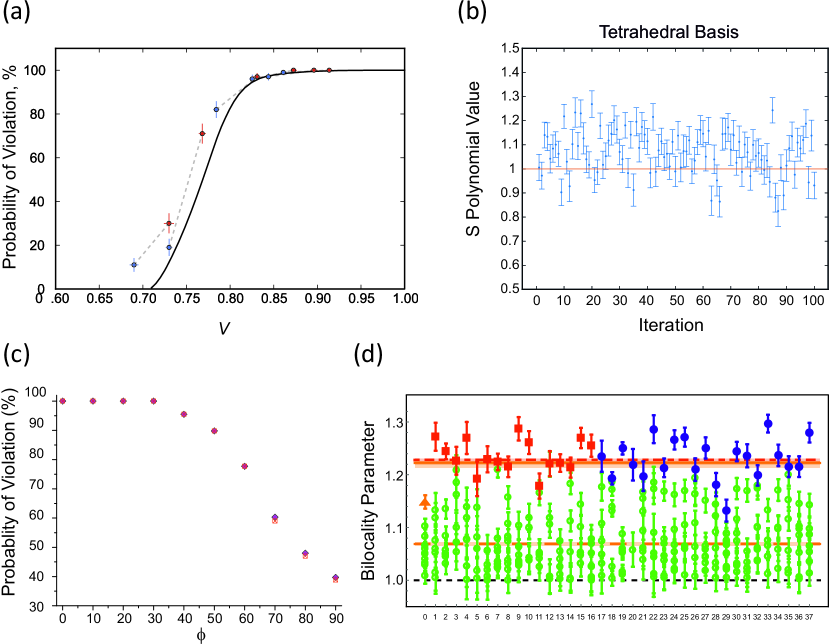
Figure 10: Experimental investigations of Bell violation with random settings. a) Increase of probability of violation (to guaranteed violation) if the fidelity of the state (quantified via visibility $V$) is increased [8]. b) Violation of Svetlichny inequality with high probability for three qubits with four tetrahedral settings each [289]. Although only $58$ of the $100$ datapoints lie at least one standard deviation above the violation threshold, about $76$ of the values themselves are above the threshold. Considering the reduced fidelity of $97\%$ the probability of violation is expected to decrease to about $69\%$, which means that the results fit the theoretical prediction very well given the experimental imperfections and uncertainty. c) Decrease of probability of violation (from guaranteed violation) if alignment of single axis is gradually lost [10]. The angle $\phi$ characterises the maximally allowed angle of misalignment of the shared axis with the maximum misalignment for $\phi=90^{\circ}$. d) Certain violation of bilocality inequality in the entanglement swapping scenario [290]. The bold datapoints correspond to different ways of introducing unitary rotations between the reference frames, with the orange triangle corresponding to just the identity operation, the red square to Haar randomly sampled directions and the blue dots to a potentially biased sampling based on random experimental parameters. For each set of unitaries the green empty circles show other non-maximal violations for different versions of the bilocality inequality.

5.8.2 Only local calibration - no alignment between parties

For the next level of randomness where any relative alignment between the parties is absent in Ref. [10] the prediction of a guaranteed violation is tested and well confirmed up to experimental imperfections. Additionally, it is explored how the scheme of using two mutually unbiased settings fails to achieve a violation with certainty as the two parties gradually loose the alignment of one common direction, see Fig. 10a. However, even in the case of total misalignment, still a violation with a probability of $42\%$ is obtained, fitting nicely with the theoretical prediction. Conversely, in Ref. [8] the scheme with triplets of mutually unbiased settings at each location (“orthogonal measurement triads”) yields a certain violation when accounting for experimental imperfections, even without any alignment. The authors additionally investigate how this probability is affected by state deterioration by artificially introducing a temporal delay in the entangling CNOT process, which reduces the coherence of the state. As shown in Fig. 10b, there exists a relatively large range of reduced coherence where a violation with almost certainty is still achieved. In the three-qubit experiment of Ref. [289], the usage of tetrahedral bases at each location achieves a violation with a probability of roughly $58\%$, as shown in Fig. 10c, which seems somewhat far away from the theoretical prediction of $88\%$. However, also this deviation is explained very well by reduced state fidelity and high statistical noise not unusual for a three-photon experiment. Finally, the entanglement swapping scenario from Ref. [290] considers three parties, $A$, $B$, and $C$, where $C$ establishes entanglement between $A$ and $B$ via a projective measurement on two qubits, each of which is entangled with a qubit at $A$ and $B$ respectively. While there is full alignment between the measurements at $A$ and the $A$-side of $C$ ($C^{A}$), both the other measurement at $C$ ($C^{B}$) and the measurement at $B$ itself have randomly rotated reference frames. As in Ref. [8], the experimental scheme of Ref. [290] involves a measurement of orthogonal triads for the two parties with randomly rotated frames $C^{B}$ and $B$. As shown in Fig. 10d, the theoretical prediction of a certain violation of the corresponding bilocality inequality is confirmed very well.

5.8.3 Complete lack of calibration

The most extreme case of randomness, when also no information about the relative orientation of local settings is present, is considered in Ref. [8] for two qubits and in Ref. [262] for the three-qubit GHZ state. The approach of Ref. [8] is to simply measure a certain number $m$ of different settings per party, where a higher number of trials simply increases the probability that a combination of settings allowing a violation will occur. Indeed, the authors show that with as little as four or five completely randomly chosen settings per party, violations will be observed with close-to-unit probability. In Ref. [262], a representative Bell-inequality and a less strict hybrid inequality, which allows for some nonlocality in the model, are experimentally tested with trials that always involve two settings per party. The authors verify that the theoretical predictions of $61.1\%$ probability of violation for the Bell inequality and $5.7\%$ for the hybrid inequality are consistent with the experimental results within the margins of error.

6 Conclusions

We reviewed foundational aspects of randomised measurements and their applications in quantum information. It was shown in detail how quantum entanglement is characterised and witnessed via statistical properties of correlations averaged over random measurement settings. This includes higher-dimensional entanglement, bound entanglement, different classes of multipartite entanglement or the number of entangled particles. The methods described are systematic with the growing complexity of analysis revealing more refined properties of entangled states. Whenever possible, theoretical criteria were discussed in parallel with their experimental implementations taking into account the effects of finite statistics. Quantum designs were also reviewed as means to simplify the implementation of averaging over random measurements.

These methods return many other characteristics of a quantum state which were illustrated with estimations of non-linear functions of density matrices including purity, fidelity, many-body topological invariants and local unitary invariants of correlation tensor, among others. Our last focus was on the role randomised measurement settings play in violation of Bell inequalities. In particular, we covered the typicality of violation, related quantifiers of non-classicality, and the impact of restricted randomness in both bipartite and multipartite scenarios.

All these results clearly demonstrate that randomised measurements are powerful theoretical and experimental tools. At the same time, they are not yet fully explored and exploited. To conclude we would like to mention a few related open problems.

The field of entanglement detection via randomised measurements has evolved towards using higher moments of the correlation distribution showing steady progress in the number and subtleties of detected entangled states. It is therefore natural to ask if given all the moments or a joint probability distribution of averaged correlations for all marginals, entanglement of any mixed state could be witnessed in a reference-frame-independent way. A similar problem is whether general LU invariance can be decided on the basis of randomised measurements only. For two qubits this is indeed possible, as we reviewed such reconstructions of Makhlin invariants, but the problem is open for higher dimensions and multipartite systems. In both situations, the complete sets of invariants are unknown and identified invariants have not been phrased explicitly in terms of randomised measurements. Moving on from the informational properties of quantum states, randomised measurements should be applied to the characterisation of quantum processes and are likely useful in other domains. A natural field is thermodynamics where information-theoretical tools have already been applied very successfully.

On the practical side, Haar randomness is the requirement of all discussed schemes. It therefore becomes important to develop methods confirming the degree of randomness realised in experiments and to construct efficient ways of generating high-dimensional Haar random unitaries. Theoretical protocols should be studied for other than Haar-random choices of settings. Finally, it is intriguing to see random measurements applied to study $k$-body marginal properties and to measure them on macroscopic quantum samples. Altogether we hope to stimulate further progress in this domain that will lead to new fundamental discoveries and practical protocols with randomised measurements.

Declaration of Competing Interest

The authors declare that they have no known competing financial interests or personal relationships that could have appeared to influence the work reported in this paper.

References

- [1] M. Munroe, D. Boggavarapu, M. E. Anderson, M. G. Raymer, Photon-number statistics from the phase-averaged quadrature-field distribution: Theory and ultrafast measurement, Phys. Rev. A 52 (1995) R924–R927. doi:10.1103/PhysRevA.52.R924.
- [2] C. W. J. Beenakker, J. W. F. Venderbos, M. P. van Exter, Two-photon speckle as a probe of multi-dimensional entanglement, Phys. Rev. Lett. 102 (2009) 193601. doi:10.1103/PhysRevLett.102.193601.
- [3] Y.-C. Liang, N. Harrigan, S. D. Bartlett, T. Rudolph, Nonclassical Correlations from Randomly Chosen Local Measurements, Phys. Rev. Lett. 104 (5) (2010) 050401. doi:10.1103/PhysRevLett.104.050401.
- [4] A. Laing, V. Scarani, J. G. Rarity, J. L. O’Brien, Reference-frame-independent quantum key distribution, Phys. Rev. A 82 (2010) 012304. doi:10.1103/PhysRevA.82.012304.
- [5] W. H. Peeters, J. J. D. Moerman, M. P. van Exter, Observation of two-photon speckle patterns, Phys. Rev. Lett. 104 (2010) 173601. doi:10.1103/PhysRevLett.104.173601.
- [6] J. J. Wallman, Y.-C. Liang, S. D. Bartlett, Generating nonclassical correlations without fully aligning measurements, Phys. Rev. A 83 (2) (2011) 022110. doi:10.1103/PhysRevA.83.022110.
- [7] S. J. van Enk, C. W. J. Beenakker, Measuring Tr(rhoˆn) on Single Copies of rho Using Random Measurements, Phys. Rev. Lett. 108 (11) (2012) 110503. doi:10.1103/PhysRevLett.108.110503.
- [8] P. Shadbolt, T. Vértesi, Y.-C. Liang, C. Branciard, N. Brunner, J. L. O’Brien, Guaranteed violation of a Bell inequality without aligned reference frames or calibrated devices, Scientific Reports 2 (1) (2012) 470. doi:10.1038/srep00470.
- [9] W. Laskowski, D. Richart, C. Schwemmer, T. Paterek, H. Weinfurter, Experimental Schmidt Decomposition and State Independent Entanglement Detection, Phys. Rev. Lett. 108 (2012) 240501. doi:10.1103/PhysRevLett.108.240501.
- [10] M. S. Palsson, J. J. Wallman, A. J. Bennet, G. J. Pryde, Experimentally demonstrating reference-frame-independent violations of Bell inequalities, Phys. Rev. A 86 (3) (2012) 032322. doi:10.1103/PhysRevA.86.032322.
-
[11]
W. Laskowski, C. Schwemmer, D. Richart, L. Knips, T. Paterek, H. Weinfurter,
Optimized state-independent
entanglement detection based on a geometrical threshold criterion, Phys.
Rev. A 88 (2) (Aug. 2013).
doi:10.1103/physreva.88.022327.
URL https://doi.org/10.1103/physreva.88.022327 - [12] A. Elben, S. T. Flammia, H.-Y. Huang, R. Kueng, J. Preskill, B. Vermersch, P. Zoller, The randomized measurement toolbox, Nature Reviews Physics 5 (1) (2022) 9–24. doi:10.1038/s42254-022-00535-2.
- [13] S. D. Bartlett, T. Rudolph, R. W. Spekkens, Classical and quantum communication without a shared reference frame, Phys. Rev. Lett. 91 (2003) 027901. doi:10.1103/PhysRevLett.91.027901.
- [14] M. Ohliger, V. Nesme, J. Eisert, Efficient and feasible state tomography of quantum many-body systems, New J. Phys. 15 (1) (2013) 015024. doi:10.1088/1367-2630/15/1/015024.
- [15] L. Knips, A moment for random measurements, Quantum Views 4 (2020) 47. doi:10.22331/qv-2020-11-19-47.
- [16] M. C. Tran, B. Dakić, F. Arnault, W. Laskowski, T. Paterek, Quantum entanglement from random measurements, Phys. Rev. A 92 (5) (2015) 050301. doi:10.1103/PhysRevA.92.050301.
- [17] M. C. Tran, B. Dakić, W. Laskowski, T. Paterek, Correlations between outcomes of random measurements, Phys. Rev. A 94 (4) (2016) 042302. doi:10.1103/PhysRevA.94.042302.
- [18] A. Ketterer, N. Wyderka, O. Gühne, Characterizing Multipartite Entanglement with Moments of Random Correlations, Phys. Rev. Lett. 122 (12) (2019) 120505. doi:10.1103/PhysRevLett.122.120505.
- [19] P. Delsarte, J.-M. Goethals, J. J. Seidel, Spherical codes and designs, in: Geometry and Combinatorics, Elsevier, 1991, pp. 68–93.
- [20] C. J. Colbourn, CRC handbook of combinatorial designs, CRC press, 2010.
- [21] N. Wyderka, Learning from correlations: What parts of quantum states tell about the whole, Phd thesis, Universität Siegen, Siegen (2020).
- [22] P. D. Seymour, T. Zaslavsky, Averaging sets: A generalization of mean values and spherical designs, Advances in Mathematics 52 (3) (1984) 213–240. doi:10.1016/0001-8708(84)90022-7.
- [23] M. A. Nielsen, I. L. Chuang, Quantum Computation and Quantum Information: 10th Anniversary Edition, Cambridge University Press, 2010. doi:10.1017/CBO9780511976667.
- [24] P. Kurzyński, T. Paterek, R. Ramanathan, W. Laskowski, D. Kaszlikowski, Correlation Complementarity Yields Bell Monogamy Relations, Phys. Rev. Lett. 106 (2011) 180402. doi:10.1103/PhysRevLett.106.180402.
- [25] O. Gamel, Entangled Bloch spheres: Bloch matrix and two-qubit state space, Phys. Rev. A 93 (6) (2016) 062320. doi:10.1103/PhysRevA.93.062320.
- [26] N. Wyderka, O. Gühne, Characterizing quantum states via sector lengths, J. Phys. A 53 (34) (2020) 345302. doi:10.1088/1751-8121/ab7f0a.
- [27] S. Morelli, C. Eltschka, M. Huber, J. Siewert, Correlation constraints and the bloch geometry of two qubits (2023). arXiv:2303.11400.
- [28] G. Kimura, The bloch vector for n-level systems, Phys. Lett. A 314 (5) (2003) 339–349. doi:10.1016/S0375-9601(03)00941-1.
- [29] M. Gell-Mann, Symmetries of Baryons and Mesons, Phys. Rev. 125 (1962) 1067–1084. doi:10.1103/PhysRev.125.1067.
- [30] J. Schlienz, G. Mahler, Description of entanglement, Phys. Rev. A 52 (1995) 4396–4404. doi:10.1103/PhysRevA.52.4396.
- [31] R. A. Bertlmann, P. Krammer, Bloch vectors for qudits, J. Phys. A 41 (23) (2008) 235303. doi:10.1088/1751-8113/41/23/235303.
- [32] A. Asadian, P. Erker, M. Huber, C. Klöckl, Heisenberg-Weyl Observables: Bloch vectors in phase space, Phys. Rev. A 94 (1) (2016) 010301. doi:10.1103/PhysRevA.94.010301.
- [33] H. Aschauer, J. Calsamiglia, M. Hein, H. J. Briegel, Local invariants for multi-partite entangled states allowing for a simple entanglement criterion, arXiv preprint quant-ph/0306048 (2003).
- [34] C. Eltschka, J. Siewert, Maximum -body correlations do not in general imply genuine multipartite entanglement, Quantum 4 (2020) 229. doi:10.22331/q-2020-02-10-229.
- [35] D. Miller, Small quantum networks in the qudit stabilizer formalism (2019). arXiv:1910.09551.
- [36] D. Kaszlikowski, A. Sen(De), U. Sen, V. Vedral, A. Winter, Quantum correlation without classical correlations, Phys. Rev. Lett. 101 (2008) 070502. doi:10.1103/PhysRevLett.101.070502.
- [37] W. Laskowski, M. Markiewicz, T. Paterek, M. Wieśniak, Incompatible local hidden-variable models of quantum correlations, Phys. Rev. A 86 (3) (September 2012). doi:10.1103/physreva.86.032105.
- [38] C. Schwemmer, L. Knips, M. C. Tran, A. de Rosier, W. Laskowski, T. Paterek, H. Weinfurter, Genuine Multipartite Entanglement without Multipartite Correlations, Phys. Rev. Lett. 114 (18) (2015) 180501. doi:10.1103/PhysRevLett.114.180501.
- [39] M. C. Tran, M. Zuppardo, A. de Rosier, L. Knips, W. Laskowski, T. Paterek, H. Weinfurter, Genuine N-partite entanglement without N-partite correlation functions, Phys. Rev. A 95 (6) (2017) 062331. doi:10.1103/PhysRevA.95.062331.
- [40] W. Kłobus, W. Laskowski, T. Paterek, M. Wieśniak, H. Weinfurter, Higher dimensional entanglement without correlations, The European Physical Journal D 73 (2) (2019) 29. doi:10.1140/epjd/e2018-90446-6.
- [41] Y. Makhlin, Nonlocal properties of two-qubit gates and mixed states, and the optimization of quantum computations, Quantum Information Processing 1 (4) (2002) 243–252. doi:10.1023/A:1022144002391.
- [42] R. Horodecki, P. Horodecki, M. Horodecki, Quantum -entropy inequalities: independent condition for local realism?, Phys. Lett. A 210 (6) (1996) 377–381. doi:10.1016/0375-9601(95)00930-2.
- [43] A. Peres, Separability Criterion for Density Matrices, Phys. Rev. Lett. 77 (8) (1996) 1413–1415. doi:10.1103/PhysRevLett.77.1413.
- [44] M. Horodecki, P. Horodecki, R. Horodecki, Separability of mixed states: necessary and sufficient conditions, Phys. Lett. A 223 (1-2) (1996) 1–8. doi:10.1016/S0375-9601(96)00706-2.
- [45] K. Życzkowski, P. Horodecki, A. Sanpera, M. Lewenstein, Volume of the set of separable states, Phys. Rev. A 58 (1998) 883–892. doi:10.1103/PhysRevA.58.883.
- [46] K. Życzkowski, Volume of the set of separable states. ii, Phys. Rev. A 60 (1999) 3496–3507. doi:10.1103/PhysRevA.60.3496.
- [47] G. Vidal, R. F. Werner, Computable measure of entanglement, Phys. Rev. A 65 (2002) 032314. doi:10.1103/PhysRevA.65.032314.
- [48] M. B. Plenio, Logarithmic negativity: A full entanglement monotone that is not convex, Phys. Rev. Lett. 95 (2005) 090503. doi:10.1103/PhysRevLett.95.090503.
- [49] J. Lee, M. S. Kim, Y. J. Park, S. Lee, Partial teleportation of entanglement in a noisy environment, Journal of Modern Optics 47 (12) (2000) 2151–2164. doi:10.1080/09500340008235138.
- [50] Y. Zhou, P. Zeng, Z. Liu, Single-Copies Estimation of Entanglement Negativity, Phys. Rev. Lett. 125 (20) (2020) 200502. doi:10.1103/PhysRevLett.125.200502.
- [51] A. Elben, R. Kueng, H.-Y. R. Huang, R. van Bijnen, C. Kokail, M. Dalmonte, P. Calabrese, B. Kraus, J. Preskill, P. Zoller, B. Vermersch, Mixed-State Entanglement from Local Randomized Measurements, Phys. Rev. Lett. 125 (20) (2020) 200501. doi:10.1103/PhysRevLett.125.200501.
- [52] S. Roman, S. Axler, F. Gehring, Advanced linear algebra, Vol. 3, Springer, 2005.
- [53] M. Curty, M. Lewenstein, N. Lütkenhaus, Entanglement as a precondition for secure quantum key distribution, Phys. Rev. Lett. 92 (2004) 217903. doi:10.1103/PhysRevLett.92.217903.
- [54] J. Gray, L. Banchi, A. Bayat, S. Bose, Machine-Learning-Assisted Many-Body Entanglement Measurement, Phys. Rev. Lett. 121 (15) (2018) 150503. doi:10.1103/PhysRevLett.121.150503.
- [55] T. Brydges, A. Elben, P. Jurcevic, B. Vermersch, C. Maier, B. P. Lanyon, P. Zoller, R. Blatt, C. F. Roos, Probing Rényi entanglement entropy via randomized measurements, Science 364 (6437) (2019) 260–263. doi:10.1126/science.aau4963.
- [56] X.-D. Yu, S. Imai, O. Gühne, Optimal Entanglement Certification from Moments of the Partial Transpose, Phys. Rev. Lett. 127 (2021) 060504. doi:10.1103/PhysRevLett.127.060504.
- [57] A. Neven, J. Carrasco, V. Vitale, C. Kokail, A. Elben, M. Dalmonte, P. Calabrese, P. Zoller, B. Vermersch, R. Kueng, B. Kraus, Symmetry-resolved entanglement detection using partial transpose moments, npj Quantum Information 7 (1) (2021) 152. doi:10.1038/s41534-021-00487-y.
- [58] J. S. Bell, On the Einstein Podolsky Rosen paradox, Physics Physique Fizika 1 (3) (1964) 195–200. doi:10.1103/PhysicsPhysiqueFizika.1.195.
- [59] J. S. Bell, The Theory of Local Beables, Epistemological Lett. 9 (1976) 11–24.
- [60] H. M. Wiseman, The two Bell’s theorems of John Bell, J. Phys. A 47 (42) (2014) 424001. doi:10.1088/1751-8113/47/42/424001.
- [61] A. Acín, N. Brunner, N. Gisin, S. Massar, S. Pironio, V. Scarani, Device-Independent Security of Quantum Cryptography against Collective Attacks, Phys. Rev. Lett. 98 (23) (June 2007). doi:10.1103/physrevlett.98.230501.
- [62] A. Acín, L. Masanes, Certified randomness in quantum physics, Nature 540 (7632) (2016) 213–219. doi:10.1038/nature20119.
- [63] H. Buhrman, R. Cleve, S. Massar, R. d. Wolf, Nonlocality and communication complexity, Reviews of Modern Physics 82 (1) (2010) 665–698. doi:10.1103/revmodphys.82.665.
- [64] N. Brunner, D. Cavalcanti, S. Pironio, V. Scarani, S. Wehner, Bell nonlocality, Reviews of Modern Physics 86 (2) (2014) 419–478. doi:10.1103/RevModPhys.86.419.
- [65] V. Scarani, Bell nonlocality, Oxford University Press, 2019.
- [66] J. F. Clauser, M. A. Horne, A. Shimony, R. A. Holt, Proposed Experiment to Test Local Hidden-Variable Theories, Phys. Rev. Lett. 23 (15) (1969) 880–884. doi:10.1103/PhysRevLett.23.880.
- [67] A. Fine, Hidden Variables, Joint Probability, and the Bell Inequalities, Phys. Rev. Lett. 48 (5) (1982) 291–295. doi:10.1103/physrevlett.48.291.
- [68] B. Hensen, H. Bernien, A. E. Dréau, A. Reiserer, N. Kalb, M. S. Blok, J. Ruitenberg, R. F. L. Vermeulen, R. N. Schouten, C. Abellán, W. Amaya, V. Pruneri, M. W. Mitchell, M. Markham, D. J. Twitchen, D. Elkouss, S. Wehner, T. H. Taminiau, R. Hanson, Loophole-free Bell inequality violation using electron spins separated by 1.3 kilometres, Nature 526 (7575) (2015) 682–686. doi:10.1038/nature15759.
- [69] M. Giustina, M. A. Versteegh, S. Wengerowsky, J. Handsteiner, A. Hochrainer, K. Phelan, F. Steinlechner, J. Kofler, J.-Å. Larsson, C. Abellán, W. Amaya, V. Pruneri, M. W. Mitchell, J. Beyer, T. Gerrits, A. E. Lita, L. K. Shalm, S. W. Nam, T. Scheidl, R. Ursin, B. Wittmann, A. Zeilinger, Significant-Loophole-Free Test of Bell’s Theorem with Entangled Photons, Phys. Rev. Lett. 115 (25) (December 2015). doi:10.1103/physrevlett.115.250401.
- [70] L. K. Shalm, E. Meyer-Scott, B. G. Christensen, P. Bierhorst, M. A. Wayne, M. J. Stevens, T. Gerrits, S. Glancy, D. R. Hamel, M. S. Allman, K. J. Coakley, S. D. Dyer, C. Hodge, A. E. Lita, V. B. Verma, C. Lambrocco, E. Tortorici, A. L. Migdall, Y. Zhang, D. R. Kumor, W. H. Farr, F. Marsili, M. D. Shaw, J. A. Stern, C. Abellán, W. Amaya, V. Pruneri, T. Jennewein, M. W. Mitchell, P. G. Kwiat, J. C. Bienfang, R. P. Mirin, E. Knill, S. W. Nam, Strong loophole-free test of local realism, Phys. Rev. Lett. 115 (25) (December 2015). doi:10.1103/physrevlett.115.250402.
- [71] W. Rosenfeld, D. Burchardt, R. Garthoff, K. Redeker, N. Ortegel, M. Rau, H. Weinfurter, Event-Ready Bell Test Using Entangled Atoms Simultaneously Closing Detection and Locality Loopholes, Phys. Rev. Lett. 119 (1) (July 2017). doi:10.1103/physrevlett.119.010402.
- [72] I. Pitovsky, Quantum Probability – Quantum Logic, Springer, Berlin, 1989.
- [73] R. F. Werner, M. M. Wolf, Bell inequalities and entanglement, Quantum Information & Computation 1 (3) (2001) 1–25.
- [74] M. Żukowski, C. Brukner, W. Laskowski, M. Wieśniak, Do All Pure Entangled States Violate Bell’s Inequalities for Correlation Functions?, Phys. Rev. Lett. 88 (2002) 210402. doi:10.1103/PhysRevLett.88.210402.
- [75] C. Śliwa, Symmetries of the Bell correlation inequalities, Phys. Lett. A 317 (3) (2003) 165–168. doi:10.1016/S0375-9601(03)01115-0.
- [76] J.-D. Bancal, N. Gisin, S. Pironio, Looking for symmetric Bell inequalities, J. Phys. A 43 (38) (2010) 385303. doi:10.1088/1751-8113/43/38/385303.
- [77] S. Pironio, All clauser–horne–shimony–holt polytopes, J. Phys. A 47 (42) (2014) 424020. doi:10.1088/1751-8113/47/42/424020.
- [78] M. Deza, M. D. Sikirić, Enumeration of the facets of cut polytopes over some highly symmetric graphs, International Transactions in Operational Research 23 (5) (2015) 853–860. doi:10.1111/itor.12194.
- [79] R. Horodecki, P. Horodecki, M. Horodecki, Violating Bell inequality by mixed spin-1/2 states: necessary and sufficient condition, Phys. Lett. A 200 (5) (1995) 340–344. doi:10.1016/0375-9601(95)00214-n.
- [80] M. Żukowski, C. Brukner, Bell’s Theorem for General N-Qubit States, Phys. Rev. Lett. 88 (21) (2002) 210401. doi:10.1103/PhysRevLett.88.210401.
- [81] O. Gühne, G. Tóth, Entanglement detection, Physics Reports 474 (1-6) (2009) 1–75. doi:10.1016/j.physrep.2009.02.004.
- [82] R. Horodecki, P. Horodecki, M. Horodecki, K. Horodecki, Quantum entanglement, Reviews of Modern Physics 81 (2) (2009) 865–942. doi:10.1103/revmodphys.81.865.
- [83] N. Friis, G. Vitagliano, M. Malik, M. Huber, Entanglement certification from theory to experiment, Nature Reviews Physics 1 (1) (2018) 72–87. doi:10.1038/s42254-018-0003-5.
- [84] M. B. Plenio, S. Virmani, An Introduction to Entanglement Measures, Quantum Info. Comput. 7 (1) (2007) 1–51, place: Paramus, NJ, Publisher: Rinton Press, Incorporated.
- [85] C. Eltschka, J. Siewert, Quantifying entanglement resources, J. Phys. A 47 (42) (2014) 424005. doi:10.1088/1751-8113/47/42/424005.
- [86] J. I. d. Vicente, Further results on entanglement detection and quantification from the correlation matrix criterion, J. Phys. A 41 (6) (2008) 065309. doi:10.1088/1751-8113/41/6/065309.
- [87] D. Bruß, G. Leuchs (Eds.), Frontmatter, John Wiley & Sons, Ltd, 2006, pp. 1–24. doi:10.1002/9783527618637.fmatter.
- [88] W. Dür, G. Vidal, J. I. Cirac, Three qubits can be entangled in two inequivalent ways, Phys. Rev. A 62 (6) (2000) 062314. doi:10.1103/PhysRevA.62.062314.
- [89] G. Tóth, Detection of multipartite entanglement in the vicinity of symmetric Dicke states, Journal of the Optical Society of America B 24 (2) (2007) 275. doi:10.1364/josab.24.000275.
- [90] H. J. Briegel, R. Raussendorf, Persistent entanglement in arrays of interacting particles, Phys. Rev. Lett. 86 (2001) 910–913. doi:10.1103/PhysRevLett.86.910.
- [91] M. Hein, J. Eisert, H. J. Briegel, Multiparty entanglement in graph states, Phys. Rev. A 69 (2004) 062311. doi:10.1103/PhysRevA.69.062311.
- [92] W. Helwig, W. Cui, J. I. Latorre, A. Riera, H.-K. Lo, Absolute maximal entanglement and quantum secret sharing, Phys. Rev. A 86 (2012) 052335. doi:10.1103/PhysRevA.86.052335.
- [93] F. Huber, O. Gühne, J. Siewert, Absolutely maximally entangled states of seven qubits do not exist, Phys. Rev. Lett. 118 (2017) 200502. doi:10.1103/PhysRevLett.118.200502.
- [94] W. Kłobus, A. Burchardt, A. Kołodziejski, M. Pandit, T. Vértesi, K. Życzkowski, W. Laskowski, -uniform mixed states, Phys. Rev. A 100 (2019) 032112. doi:10.1103/PhysRevA.100.032112.
- [95] S. Gharibian, Strong NP-hardness of the quantum separability problem, Quantum Information & Computation 10 (3 & 4) (2010) 343–360.
- [96] J. de Pillis, Linear transformations which preserve hermitian and positive semidefinite operators, Pacific Journal of Mathematics 23 (1) (1967) 129–137.
- [97] M.-D. Choi, Completely positive linear maps on complex matrices, Linear Algebra and its Applications 10 (3) (1975) 285–290. doi:10.1016/0024-3795(75)90075-0.
- [98] A. Jamiołkowski, Linear transformations which preserve trace and positive semidefiniteness of operators, Reports on Mathematical Physics 3 (4) (1972) 275–278. doi:10.1016/0034-4877(72)90011-0.
- [99] M. Lewenstein, B. Kraus, J. I. Cirac, P. Horodecki, Optimization of entanglement witnesses, Phys. Rev. A 62 (2000) 052310. doi:10.1103/PhysRevA.62.052310.
- [100] D. Bruß, J. I. Cirac, P. Horodecki, F. Hulpke, B. Kraus, M. Lewenstein, A. Sanpera, Reflections upon separability and distillability, Journal of Modern Optics 49 (8) (2002) 1399–1418. doi:10.1080/09500340110105975.
- [101] A. Acín, N. Gisin, L. Masanes, From Bell’s Theorem to Secure Quantum Key Distribution, Phys. Rev. Lett. 97 (2006) 120405. doi:10.1103/PhysRevLett.97.120405.
- [102] J.-D. Bancal, N. Gisin, Y.-C. Liang, S. Pironio, Device-independent witnesses of genuine multipartite entanglement, Phys. Rev. Lett. 106 (2011) 250404. doi:10.1103/PhysRevLett.106.250404.
- [103] K. F. Pál, T. Vértesi, M. Navascués, Device-independent tomography of multipartite quantum states, Phys. Rev. A 90 (2014) 042340. doi:10.1103/PhysRevA.90.042340.
- [104] A. Sørensen, L.-M. Duan, J. I. Cirac, P. Zoller, Many-particle entanglement with Bose–Einstein condensates, Nature 409 (6816) (2001) 63–66. doi:10.1038/35051038.
- [105] G. Tóth, C. Knapp, O. Gühne, H. J. Briegel, Optimal spin squeezing inequalities detect bound entanglement in spin models, Phys. Rev. Lett. 99 (2007) 250405. doi:10.1103/PhysRevLett.99.250405.
- [106] J. Ma, X. Wang, C. Sun, F. Nori, Quantum spin squeezing, Physics Reports 509 (2) (2011) 89–165. doi:10.1016/j.physrep.2011.08.003.
- [107] N. J. Cerf, C. Adami, Negative entropy and information in quantum mechanics, Phys. Rev. Lett. 79 (1997) 5194–5197. doi:10.1103/PhysRevLett.79.5194.
- [108] M. Horodecki, J. Oppenheim, A. Winter, Partial quantum information, Nature 436 (7051) (2005) 673–676.
- [109] V. Coffman, J. Kundu, W. K. Wootters, Distributed entanglement, Phys. Rev. A 61 (2000) 052306. doi:10.1103/PhysRevA.61.052306.
- [110] T. J. Osborne, F. Verstraete, General monogamy inequality for bipartite qubit entanglement, Phys. Rev. Lett. 96 (2006) 220503. doi:10.1103/PhysRevLett.96.220503.
- [111] M. Horodecki, P. Horodecki, R. Horodecki, Mixed-state entanglement and distillation: Is there a “bound” entanglement in nature?, Phys. Rev. Lett. 80 (1998) 5239–5242. doi:10.1103/PhysRevLett.80.5239.
- [112] D. P. DiVincenzo, P. W. Shor, J. A. Smolin, B. M. Terhal, A. V. Thapliyal, Evidence for bound entangled states with negative partial transpose, Phys. Rev. A 61 (2000) 062312. doi:10.1103/PhysRevA.61.062312.
- [113] C. H. Bennett, G. Brassard, C. Crépeau, R. Jozsa, A. Peres, W. K. Wootters, Teleporting an unknown quantum state via dual classical and einstein-podolsky-rosen channels, Phys. Rev. Lett. 70 (1993) 1895–1899. doi:10.1103/PhysRevLett.70.1895.
- [114] M. Horodecki, J. Oppenheim, A. Winter, Quantum State Merging and Negative Information, Communications in Mathematical Physics 269 (1) (2006) 107–136. doi:10.1007/s00220-006-0118-x.
- [115] L. Pezzé, A. Smerzi, Entanglement, Nonlinear Dynamics, and the Heisenberg Limit, Phys. Rev. Lett. 102 (2009) 100401. doi:10.1103/PhysRevLett.102.100401.
- [116] G. Tóth, I. Apellaniz, Quantum metrology from a quantum information science perspective, J. Phys. A 47 (42) (2014) 424006. doi:10.1088/1751-8113/47/42/424006.
- [117] L. Pezzè, A. Smerzi, M. K. Oberthaler, R. Schmied, P. Treutlein, Quantum metrology with nonclassical states of atomic ensembles, Reviews of Modern Physics 90 (2018) 035005. doi:10.1103/RevModPhys.90.035005.
- [118] W. Dür, J. I. Cirac, R. Tarrach, Separability and Distillability of Multiparticle Quantum Systems, Phys. Rev. Lett. 83 (17) (1999) 3562–3565. doi:10.1103/PhysRevLett.83.3562.
- [119] W. Dür, J. I. Cirac, Classification of multiqubit mixed states: Separability and distillability properties, Phys. Rev. A 61 (4) (March 2000). doi:10.1103/physreva.61.042314.
- [120] O. Gühne, G. Tóth, H. J. Briegel, Multipartite entanglement in spin chains, New J. Phys. 7 (2005) 229–229. doi:10.1088/1367-2630/7/1/229.
- [121] O. Gühne, G. Tóth, Energy and multipartite entanglement in multidimensional and frustrated spin models, Phys. Rev. A 73 (5) (May 2006). doi:10.1103/physreva.73.052319.
- [122] P. Hyllus, W. Laskowski, R. Krischek, C. Schwemmer, W. Wieczorek, H. Weinfurter, L. Pezzé, A. Smerzi, Fisher information and multiparticle entanglement, Phys. Rev. A 85 (2) (February 2012). doi:10.1103/physreva.85.022321.
- [123] A. S. Sørensen, K. Mølmer, Entanglement and Extreme Spin Squeezing, Phys. Rev. Lett. 86 (20) (2001) 4431–4434. doi:10.1103/physrevlett.86.4431.
- [124] S. Szalay, k-stretchability of entanglement, and the duality of k-separability and k-producibility, Quantum 3 (2019) 204. doi:10.22331/q-2019-12-02-204.
- [125] G. Tóth, Stretching the limits of multiparticle entanglement, Quantum Views 4 (2020) 30. doi:10.22331/qv-2020-01-27-30.
- [126] Z. Ren, W. Li, A. Smerzi, M. Gessner, Metrological detection of multipartite entanglement from young diagrams, Phys. Rev. Lett. 126 (2021) 080502. doi:10.1103/PhysRevLett.126.080502.
- [127] J. Eisert, H. J. Briegel, Schmidt measure as a tool for quantifying multiparticle entanglement, Phys. Rev. A 64 (2001) 022306. doi:10.1103/PhysRevA.64.022306.
- [128] C. Spengler, M. Huber, A. Gabriel, B. C. Hiesmayr, Examining the dimensionality of genuine multipartite entanglement, Quantum information processing 12 (2013) 269–278.
- [129] M. Huber, J. I. de Vicente, Structure of multidimensional entanglement in multipartite systems, Phys. Rev. Lett. 110 (2013) 030501. doi:10.1103/PhysRevLett.110.030501.
- [130] T. Kraft, C. Ritz, N. Brunner, M. Huber, O. Gühne, Characterizing genuine multilevel entanglement, Phys. Rev. Lett. 120 (2018) 060502. doi:10.1103/PhysRevLett.120.060502.
- [131] M. Navascués, E. Wolfe, D. Rosset, A. Pozas-Kerstjens, Genuine network multipartite entanglement, Phys. Rev. Lett. 125 (2020) 240505. doi:10.1103/PhysRevLett.125.240505.
- [132] A. Tavakoli, A. Pozas-Kerstjens, M.-X. Luo, M.-O. Renou, Bell nonlocality in networks, Reports on Progress in Physics 85 (5) (2022) 056001. doi:10.1088/1361-6633/ac41bb.
- [133] K. Hansenne, Z.-P. Xu, T. Kraft, O. Guehne, Symmetries in quantum networks lead to no-go theorems for entanglement distribution and to verification techniques, Nature Communications 13 (1) (jan 2022). doi:10.1038/s41467-022-28006-3.
- [134] B. Collins, P. Śniady, Integration with Respect to the Haar Measure on Unitary, Orthogonal and Symplectic Group, Communications in Mathematical Physics 264 (3) (2006) 773–795. doi:10.1007/s00220-006-1554-3.
- [135] Z. Puchała, J. A. Miszczak, Symbolic integration with respect to the Haar measure on the unitary groups, Bulletin of the Polish Academy of Sciences Technical Sciences 65 (1) (2017) 21–27. doi:10.1515/bpasts-2017-0003.
- [136] C. Spengler, M. Huber, B. C. Hiesmayr, Composite parameterization and Haar measure for all unitary and special unitary groups, Journal of Mathematical Physics 53 (1) (2012) 013501. doi:10.1063/1.3672064.
- [137] L. Zhang, Matrix integrals over unitary groups: An application of Schur-Weyl duality (2015). arXiv:1408.3782.
- [138] B. Collins, S. Matsumoto, J. Novak, The weingarten calculus (2021). arXiv:2109.14890.
- [139] T. Tilma, E. C. G. Sudarshan, Generalized Euler angle parametrization for SU(N), J. Phys. A 35 (48) (2002) 10467. doi:10.1088/0305-4470/35/48/316.
- [140] J. J. Sakurai, E. D. Commins, Modern quantum mechanics, revised edition (1995).
- [141] K. Horodecki, M. Horodecki, P. Horodecki, D. Leung, J. Oppenheim, Quantum key distribution based on private states: Unconditional security over untrusted channels with zero quantum capacity, IEEE Transactions on Information Theory 54 (6) (2008) 2604–2620. doi:10.1109/TIT.2008.921870.
- [142] N. Wyderka, A. Ketterer, S. Imai, J. L. Bönsel, D. E. Jones, B. T. Kirby, X.-D. Yu, O. Gühne, Complete characterization of quantum correlations by randomized measurements (2022). doi:10.48550/ARXIV.2212.07894.
- [143] S. Imai, N. Wyderka, A. Ketterer, O. Gühne, Bound Entanglement from Randomized Measurements, Phys. Rev. Lett. 126 (15) (2021) 150501. doi:10.1103/PhysRevLett.126.150501.
- [144] N. Wyderka, A. Ketterer, Probing the geometry of correlation matrices with randomized measurements, PRX Quantum 4 (2023) 020325. doi:10.1103/PRXQuantum.4.020325.
- [145] E. Bannai, E. Bannai, A survey on spherical designs and algebraic combinatorics on spheres, European Journal of Combinatorics 30 (6) (2009) 1392–1425. doi:10.1016/j.ejc.2008.11.007.
- [146] R. H. Hardin, N. J. A. Sloane, McLaren’s Improved Snub Cube and Other New Spherical Designs in Three Dimensions (2002). arXiv:math/0207211.
- [147] J. M. Renes, R. Blume-Kohout, A. J. Scott, C. M. Caves, Symmetric informationally complete quantum measurements, Journal of Mathematical Physics 45 (6) (2004) 2171–2180. doi:10.1063/1.1737053.
- [148] A. Ambainis, J. Emerson, Quantum t-designs: t-wise independence in the quantum world (2007). arXiv:quant-ph/0701126.
- [149] I. Bengtsson, K. Życzkowski, Geometry of Quantum States: An Introduction to Quantum Entanglement, 2nd Edition, Cambridge University Press, 2017. doi:10.1017/9781139207010.
- [150] W. K. Wootters, Statistical distance and Hilbert space, Phys. Rev. D 23 (1981) 357–362. doi:10.1103/PhysRevD.23.357.
- [151] A. Barenco, A. Berthiaume, D. Deutsch, A. Ekert, R. Jozsa, C. Macchiavello, Stabilization of quantum computations by symmetrization, SIAM Journal on Computing 26 (5) (1997) 1541–1557. doi:10.1137/S0097539796302452.
- [152] A. W. Harrow, The church of the symmetric subspace (2013). arXiv:1308.6595.
- [153] F. G. S. L. Brandao, M. Christandl, A. W. Harrow, M. Walter, The mathematics of entanglement (2016). arXiv:1604.01790.
- [154] R. A. Low, Pseudo-randomness and learning in quantum computation (2010). arXiv:1006.5227.
- [155] A. Ketterer, O. Gühne, Entropic uncertainty relations from quantum designs, Phys. Rev. Res. 2 (2) (2020) 023130. doi:10.1103/PhysRevResearch.2.023130.
- [156] L. Welch, Lower bounds on the maximum cross correlation of signals (corresp.), IEEE Transactions on Information Theory 20 (3) (1974) 397–399. doi:10.1109/TIT.1974.1055219.
- [157] A. Klappenecker, M. Roetteler, Mutually unbiased bases are complex projective 2-designs (2005). arXiv:quant-ph/0502031.
- [158] T. Durt, B.-G. Englert, I. Bengtsson, K. Życzkowski, On Mutually Unbiased Bases, International Journal of Quantum Information 08 (04) (2010) 535–640. doi:10.1142/S0219749910006502.
- [159] P. Horodecki, L. Rudnicki, K. Życzkowski, Five open problems in quantum information theory, PRX Quantum 3 (2022) 010101. doi:10.1103/PRXQuantum.3.010101.
- [160] M. Weiner, A gap for the maximum number of mutually unbiased bases (2010). doi:10.48550/arXiv.0902.0635.
- [161] I. D. Ivonovic, Geometrical description of quantal state determination, J. Phys. A 14 (12) (1981) 3241. doi:10.1088/0305-4470/14/12/019.
- [162] W. K. Wootters, B. D. Fields, Optimal state-determination by mutually unbiased measurements, Annals of Physics 191 (2) (1989) 363–381. doi:10.1016/0003-4916(89)90322-9.
- [163] M. Wieśniak, T. Paterek, A. Zeilinger, Entanglement in mutually unbiased bases, New J. Phys. 13 (5) (2011) 053047. doi:10.1088/1367-2630/13/5/053047.
- [164] U. Seyfarth, K. S. Ranade, Construction of mutually unbiased bases with cyclic symmetry for qubit systems, Phys. Rev. A 84 (2011) 042327. doi:10.1103/PhysRevA.84.042327.
-
[165]
G. Zauner, Grundzuege
einer nichtkommutativen Designtheorie, Ph. D. dissertation, PhD thesis
(1999).
URL https://www.mat.univie.ac.at/~neum/ms/zauner.pdf - [166] D. Gross, K. Audenaert, J. Eisert, Evenly distributed unitaries: On the structure of unitary designs, Journal of Mathematical Physics 48 (5) (05 2007). doi:10.1063/1.2716992.
- [167] C. Dankert, R. Cleve, J. Emerson, E. Livine, Exact and approximate unitary 2-designs and their application to fidelity estimation, Phys. Rev. A 80 (2009) 012304. doi:10.1103/PhysRevA.80.012304.
- [168] A. J. Scott, Optimizing quantum process tomography with unitary 2-designs, J. Phys. A 41 (5) (2008) 055308. doi:10.1088/1751-8113/41/5/055308.
- [169] D. A. Roberts, B. Yoshida, Chaos and complexity by design, Journal of High Energy Physics 2017 (4) (apr 2017). doi:10.1007/jhep04(2017)121.
- [170] G. Köstenberger, Weingarten calculus (2021). arXiv:2101.00921.
- [171] K. G. H. Vollbrecht, R. F. Werner, Entanglement measures under symmetry, Phys. Rev. A 64 (2001) 062307. doi:10.1103/PhysRevA.64.062307.
- [172] T. Eggeling, R. F. Werner, Separability properties of tripartite states with symmetry, Phys. Rev. A 63 (2001) 042111. doi:10.1103/PhysRevA.63.042111.
- [173] R. F. Werner, Quantum states with Einstein-Podolsky-Rosen correlations admitting a hidden-variable model, Phys. Rev. A 40 (1989) 4277–4281. doi:10.1103/PhysRevA.40.4277.
- [174] P. Horodecki, A. Ekert, Method for direct detection of quantum entanglement, Phys. Rev. Lett. 89 (2002) 127902. doi:10.1103/PhysRevLett.89.127902.
- [175] A. K. Ekert, C. M. Alves, D. K. L. Oi, M. Horodecki, P. Horodecki, L. C. Kwek, Direct estimations of linear and nonlinear functionals of a quantum state, Phys. Rev. Lett. 88 (2002) 217901. doi:10.1103/PhysRevLett.88.217901.
- [176] A. W. Harrow, R. A. Low, Random Quantum Circuits are Approximate 2-designs, Communications in Mathematical Physics 291 (1) (2009) 257–302. doi:10.1007/s00220-009-0873-6.
- [177] F. Huber, Positive maps and trace polynomials from the symmetric group, Journal of Mathematical Physics 62 (2) (02 2021). doi:10.1063/5.0028856.
- [178] F. Huber, N. Wyderka, Refuting spectral compatibility of quantum marginals (2023). arXiv:2211.06349.
- [179] A. Rico, F. Huber, Entanglement detection with trace polynomials (2023). arXiv:2303.07761.
- [180] R. J. Garcia, Y. Zhou, A. Jaffe, Quantum scrambling with classical shadows, Phys. Rev. Res. 3 (3) (August 2021). doi:10.1103/physrevresearch.3.033155.
- [181] F. G. Brandão, W. Chemissany, N. Hunter-Jones, R. Kueng, J. Preskill, Models of quantum complexity growth, PRX Quantum 2 (2021) 030316. doi:10.1103/PRXQuantum.2.030316.
- [182] N. Hunter-Jones, J. Liu, Chaos and random matrices in supersymmetric SYK, Journal of High Energy Physics 2018 (5) (2018) 1–26.
- [183] A. Roy, A. J. Scott, Unitary designs and codes, Designs, Codes and Cryptography 53 (1) (2009) 13–31. doi:10.1007/s10623-009-9290-2.
- [184] Z. Webb, The clifford group forms a unitary 3-design (2016). doi:10.48550/arXiv.1510.02769.
- [185] H. Zhu, R. Kueng, M. Grassl, D. Gross, The clifford group fails gracefully to be a unitary 4-design (2016). doi:10.48550/arXiv.1609.08172.
- [186] A. S. M. Hassan, P. S. Joag, Separability criterion for multipartite quantum states based on the bloch representation of density matrices (2008). arXiv:0704.3942.
- [187] A. S. M. Hassan, P. S. Joag, Experimentally accessible geometric measure for entanglement in -qubit pure states, Phys. Rev. A 77 (2008) 062334. doi:10.1103/PhysRevA.77.062334.
- [188] A. S. M. Hassan, P. S. Joag, Geometric measure for entanglement in N-qudit pure states, Phys. Rev. A 80 (4) (2009) 042302. doi:10.1103/PhysRevA.80.042302.
- [189] M. A. Nielsen, Conditions for a Class of Entanglement Transformations, Phys. Rev. Lett. 83 (2) (1999) 436–439. doi:10.1103/physrevlett.83.436.
- [190] R. Horodecki, M. Horodecki, Information-theoretic aspects of inseparability of mixed states, Phys. Rev. A 54 (3) (1996) 1838–1843. doi:10.1103/PhysRevA.54.1838.
- [191] W. Dür, J. I. Cirac, Multiparticle entanglement and its experimental detection, J. Phys. A 34 (35) (2001) 6837. doi:10.1088/0305-4470/34/35/310.
- [192] O. Gühne, B. Jungnitsch, T. Moroder, Y. S. Weinstein, Multiparticle entanglement in graph-diagonal states: Necessary and sufficient conditions for four qubits, Phys. Rev. A 84 (2011) 052319. doi:10.1103/PhysRevA.84.052319.
- [193] C. Eltschka, J. Siewert, Entanglement of Three-Qubit Greenberger-Horne-Zeilinger–Symmetric States, Phys. Rev. Lett. 108 (2012) 020502. doi:10.1103/PhysRevLett.108.020502.
- [194] R. Augusiak, M. Demianowicz, P. Horodecki, Universal observable detecting all two-qubit entanglement and determinant-based separability tests, Phys. Rev. A 77 (3) (2008) 030301. doi:10.1103/PhysRevA.77.030301.
- [195] T. Lawson, A. Pappa, B. Bourdoncle, I. Kerenidis, D. Markham, E. Diamanti, Reliable experimental quantification of bipartite entanglement without reference frames, Phys. Rev. A 90 (4) (2014) 042336. doi:10.1103/PhysRevA.90.042336.
- [196] S. Hill, W. K. Wootters, Entanglement of a pair of quantum bits, Phys. Rev. Lett. 78 (26) (1997) 5022–h–5025. doi:10.1103/physrevlett.78.5022.
- [197] A. Elben, B. Vermersch, M. Dalmonte, J. I. Cirac, P. Zoller, Rényi Entropies from Random Quenches in Atomic Hubbard and Spin Models, Phys. Rev. Lett. 120 (5) (2018) 050406. doi:10.1103/PhysRevLett.120.050406.
- [198] S. Imai, O. Gühne, S. Nimmrichter, Work fluctuations and entanglement in quantum batteries, Phys. Rev. A 107 (2023) 022215. doi:10.1103/PhysRevA.107.022215.
- [199] K. G. H. Vollbrecht, M. M. Wolf, Conditional entropies and their relation to entanglement criteria, Journal of Mathematical Physics 43 (9) (2002) 4299–4306. doi:10.1063/1.1498490.
- [200] O. Gühne, M. Lewenstein, Entropic uncertainty relations and entanglement, Phys. Rev. A 70 (2004) 022316. doi:10.1103/PhysRevA.70.022316.
- [201] T. Hiroshima, Majorization criterion for distillability of a bipartite quantum state, Phys. Rev. Lett. 91 (2003) 057902. doi:10.1103/PhysRevLett.91.057902.
- [202] J. de Vicente, Separability criteria based on the Bloch representation of density matrices, Quantum Information and Computation 7 (7) (2007) 624–638. doi:10.26421/QIC7.7-5.
- [203] S. Liu, Q. He, M. Huber, O. Gühne, G. Vitagliano, Characterizing entanglement dimensionality from randomized measurements (2022). arXiv:2211.09614.
- [204] D. Bruß, A. Peres, Construction of quantum states with bound entanglement, Phys. Rev. A 61 (2000) 030301. doi:10.1103/PhysRevA.61.030301.
- [205] in preparation.
- [206] M. Markiewicz, W. Laskowski, T. Paterek, M. Żukowski, Detecting genuine multipartite entanglement of pure states with bipartite correlations, Phys. Rev. A 87 (2013) 034301. doi:10.1103/PhysRevA.87.034301.
- [207] C. Klöckl, M. Huber, Characterizing multipartite entanglement without shared reference frames, Phys. Rev. A 91 (4) (2015) 042339. doi:10.1103/PhysRevA.91.042339.
- [208] F. Huber, S. Severini, Some ulam’s reconstruction problems for quantum states, J. Phys. A 51 (43) (2018) 435301. doi:10.1088/1751-8121/aadd1e.
- [209] D. Miller, D. Loss, I. Tavernelli, H. Kampermann, D. Bruß, N. Wyderka, Sector length distributions of graph states (2022). doi:10.48550/arXiv.2207.07665.
- [210] A. Ketterer, S. Imai, N. Wyderka, O. Gühne, Statistically significant tests of multiparticle quantum correlations based on randomized measurements, Phys. Rev. A 106 (1) (July 2022). doi:10.1103/physreva.106.l010402.
- [211] R. Lohmayer, A. Osterloh, J. Siewert, A. Uhlmann, Entangled three-qubit states without concurrence and three-tangle, Phys. Rev. Lett. 97 (2006) 260502. doi:10.1103/PhysRevLett.97.260502.
- [212] L. Knips, J. Dziewior, W. Kłobus, W. Laskowski, T. Paterek, P. J. Shadbolt, H. Weinfurter, J. D. A. Meinecke, Multipartite entanglement analysis from random correlations, npj Quantum Information 6 (1) (2020) 51. doi:10.1038/s41534-020-0281-5.
- [213] L. Knips, C. Schwemmer, N. Klein, M. Wieśniak, H. Weinfurter, Multipartite Entanglement Detection with Minimal Effort, Phys. Rev. Lett. 117 (21) (2016) 210504. doi:10.1103/PhysRevLett.117.210504.
- [214] E. Chitambar, G. Gour, Quantum resource theories, Reviews of Modern Physics 91 (2019) 025001. doi:10.1103/RevModPhys.91.025001.
- [215] A. Acín, D. Bruß, M. Lewenstein, A. Sanpera, Classification of Mixed Three-Qubit States, Phys. Rev. Lett. 87 (4) (2001) 040401. doi:10.1103/PhysRevLett.87.040401.
- [216] R. Cleve, D. Gottesman, H.-K. Lo, How to share a quantum secret, Phys. Rev. Lett. 83 (1999) 648–651. doi:10.1103/PhysRevLett.83.648.
- [217] R. Raussendorf, H. J. Briegel, A one-way quantum computer, Phys. Rev. Lett. 86 (2001) 5188–5191. doi:10.1103/PhysRevLett.86.5188.
- [218] A. I. Lvovsky, B. C. Sanders, W. Tittel, Optical quantum memory, Nature Photonics 3 (12) (2009) 706–714. doi:10.1038/nphoton.2009.231.
- [219] F. Verstraete, J. Dehaene, B. De Moor, H. Verschelde, Four qubits can be entangled in nine different ways, Phys. Rev. A 65 (2002) 052112. doi:10.1103/PhysRevA.65.052112.
- [220] A. Ketterer, N. Wyderka, O. Gühne, Entanglement characterization using quantum designs, Quantum 4 (2020) 325. doi:10.22331/q-2020-09-16-325.
- [221] S. T. Flammia, Y.-K. Liu, Direct fidelity estimation from few pauli measurements, Phys. Rev. Lett. 106 (2011) 230501. doi:10.1103/PhysRevLett.106.230501.
- [222] S. Pallister, N. Linden, A. Montanaro, Optimal verification of entangled states with local measurements, Phys. Rev. Lett. 120 (2018) 170502. doi:10.1103/PhysRevLett.120.170502.
- [223] A. Elben, B. Vermersch, C. F. Roos, P. Zoller, Statistical correlations between locally randomized measurements: A toolbox for probing entanglement in many-body quantum states, Phys. Rev. A 99 (5) (2019) 052323. doi:10.1103/PhysRevA.99.052323.
- [224] A. Elben, B. Vermersch, R. van Bijnen, C. Kokail, T. Brydges, C. Maier, M. K. Joshi, R. Blatt, C. F. Roos, P. Zoller, Cross-Platform Verification of Intermediate Scale Quantum Devices, Phys. Rev. Lett. 124 (1) (2020) 010504. doi:10.1103/PhysRevLett.124.010504.
- [225] X.-D. Yu, J. Shang, O. Gühne, Statistical methods for quantum state verification and fidelity estimation, Advanced Quantum Technologies 5 (5) (2022) 2100126. doi:10.1002/qute.202100126.
- [226] A. Dimić, B. Dakić, Single-copy entanglement detection, npj Quantum Information 4 (1) (2018) 11. doi:10.1038/s41534-017-0055-x.
- [227] V. Saggio, A. Dimić, C. Greganti, L. A. Rozema, P. Walther, B. Dakić, Experimental few-copy multipartite entanglement detection, Nature Physics 15 (9) (2019) 935–940. doi:10.1038/s41567-019-0550-4.
- [228] P. Cieśliński, J. Dziewior, L. Knips, W. Kłobus, J. Meinecke, T. Paterek, H. Weinfurter, W. Laskowski, High validity entanglement verification with finite copies of a quantum state, arXiv (2022). doi:10.48550/arXiv.2208.01983.
- [229] Y.-C. Liang, Y.-H. Yeh, P. E. M. F. Mendonça, R. Y. Teh, M. D. Reid, P. D. Drummond, Quantum fidelity measures for mixed states, Reports on Progress in Physics 82 (7) (2019) 076001. doi:10.1088/1361-6633/ab1ca4.
- [230] R. Jozsa, Fidelity for mixed quantum states, Journal of Modern Optics 41 (12) (1994) 2315–2323. doi:10.1080/09500349414552171.
- [231] A. Uhlmann, The “transition probability” in the state space of a -algebra, Reports on Mathematical Physics 9 (2) (1976) 273–279. doi:10.1016/0034-4877(76)90060-4.
- [232] A. Elben, J. Yu, G. Zhu, M. Hafezi, F. Pollmann, P. Zoller, B. Vermersch, Many-body topological invariants from randomized measurements in synthetic quantum matter, Science Advances 6 (15) (2020) eaaz3666. doi:10.1126/sciadv.aaz3666.
- [233] F. Pollmann, A. M. Turner, Detection of symmetry-protected topological phases in one dimension, Phys. Rev. B 86 (12) (2012) 125441. doi:10.1103/PhysRevB.86.125441.
-
[234]
F. Mezzadri, How to generate random
matrices from the classical compact groups, arXiv:math-ph/0609050 (February
2007).
URL http://arxiv.org/abs/math-ph/0609050 - [235] R. Nandkishore, D. A. Huse, Many-body localization and thermalization in quantum statistical mechanics, Annual Review of Condensed Matter Physics 6 (1) (2015) 15–38. doi:10.1146/annurev-conmatphys-031214-014726.
- [236] C. W. Helstrom, Quantum detection and estimation theory, Journal of Statistical Physics 1 (2) (1969) 231–252. doi:10.1007/bf01007479.
- [237] S. L. Braunstein, C. M. Caves, Statistical distance and the geometry of quantum states, Phys. Rev. Lett. 72 (1994) 3439–3443. doi:10.1103/PhysRevLett.72.3439.
- [238] J. Liu, H. Yuan, X.-M. Lu, X. Wang, Quantum fisher information matrix and multiparameter estimation, J. Phys. A 53 (2) (2019) 023001. doi:10.1088/1751-8121/ab5d4d.
- [239] M. Yu, D. Li, J. Wang, Y. Chu, P. Yang, M. Gong, N. Goldman, J. Cai, Experimental estimation of the quantum fisher information from randomized measurements, Phys. Rev. Res. 3 (2021) 043122. doi:10.1103/PhysRevResearch.3.043122.
- [240] A. Rath, C. Branciard, A. Minguzzi, B. Vermersch, Quantum Fisher Information from Randomized Measurements, Phys. Rev. Lett. 127 (26) (2021) 260501. doi:10.1103/PhysRevLett.127.260501.
- [241] X. Nie, Z. Zhang, X. Zhao, T. Xin, D. Lu, J. Li, Detecting scrambling via statistical correlations between randomized measurements on an nmr quantum simulator (2019). arXiv:1903.12237.
-
[242]
M. K. Joshi, A. Elben, B. Vermersch, T. Brydges, C. Maier, P. Zoller, R. Blatt,
C. F. Roos, Quantum
Information Scrambling in a Trapped-Ion Quantum Simulator with
Tunable Range Interactions, Phys. Rev. Lett. 124 (24) (June 2020).
URL https://doi.org/10.1103/physrevlett.124.240505 - [243] H.-Y. Huang, R. Kueng, J. Preskill, Predicting many properties of a quantum system from very few measurements, Nature Physics 16 (10) (2020) 1050–1057. doi:10.1038/s41567-020-0932-7.
- [244] M. Horodecki, P. Horodecki, R. Horodecki, General teleportation channel, singlet fraction, and quasidistillation, Phys. Rev. A 60 (1999) 1888–1898. doi:10.1103/PhysRevA.60.1888.
- [245] O. Gühne, Y. Mao, X.-D. Yu, Geometry of faithful entanglement, Phys. Rev. Lett. 126 (2021) 140503. doi:10.1103/PhysRevLett.126.140503.
- [246] D. F. V. James, P. G. Kwiat, W. J. Munro, A. G. White, Measurement of qubits, Phys. Rev. A 64 (2001) 052312. doi:10.1103/PhysRevA.64.052312.
- [247] G. M. D’Ariano, M. G. Paris, M. F. Sacchi, Quantum tomography, Advances in imaging and electron physics 128 (2003) 206–309. doi:10.48550/arXiv.quant-ph/0302028.
- [248] M. Paris, J. Rehacek, Quantum state estimation, Vol. 649, Springer Science & Business Media, 2004. doi:10.1007/b98673.
- [249] M. Cramer, M. B. Plenio, S. T. Flammia, R. Somma, D. Gross, S. D. Bartlett, O. Landon-Cardinal, D. Poulin, Y.-K. Liu, Efficient quantum state tomography, Nature Communications 1 (1) (December 2010). doi:10.1038/ncomms1147.
- [250] D. Gross, Y.-K. Liu, S. T. Flammia, S. Becker, J. Eisert, Quantum state tomography via compressed sensing, Phys. Rev. Lett. 105 (2010) 150401. doi:10.1103/PhysRevLett.105.150401.
- [251] G. Tóth, W. Wieczorek, D. Gross, R. Krischek, C. Schwemmer, H. Weinfurter, Permutationally invariant quantum tomography, Phys. Rev. Lett. 105 (2010) 250403. doi:10.1103/PhysRevLett.105.250403.
- [252] T. Moroder, P. Hyllus, G. Tóth, C. Schwemmer, A. Niggebaum, S. Gaile, O. Gühne, H. Weinfurter, Permutationally invariant state reconstruction, New J. Phys. 14 (10) (2012) 105001. doi:10.1088/1367-2630/14/10/105001.
- [253] S. Aaronson, Shadow tomography of quantum states, SIAM Journal on Computing 49 (5) (2020) STOC18–368–STOC18–394. doi:10.1137/18M120275X.
- [254] H. C. Nguyen, J. L. Bönsel, J. Steinberg, O. Gühne, Optimizing Shadow Tomography with Generalized Measurements, Phys. Rev. Lett. 129 (22) (2022) 220502. doi:10.1103/PhysRevLett.129.220502.
- [255] C. M. Bishop, N. M. Nasrabadi, Pattern recognition and machine learning, Springer, 2006.
- [256] T. Zhang, J. Sun, X.-X. Fang, X.-M. Zhang, X. Yuan, H. Lu, Experimental quantum state measurement with classical shadows, Phys. Rev. Lett. 127 (20) (November 2021). doi:10.1103/physrevlett.127.200501.
- [257] G. Struchalin, Y. A. Zagorovskii, E. Kovlakov, S. Straupe, S. Kulik, Experimental estimation of quantum state properties from classical shadows, PRX Quantum 2 (2021) 010307. doi:10.1103/PRXQuantum.2.010307.
- [258] R. Stricker, M. Meth, L. Postler, C. Edmunds, C. Ferrie, R. Blatt, P. Schindler, T. Monz, R. Kueng, M. Ringbauer, Experimental single-setting quantum state tomography, PRX Quantum 3 (2022) 040310. doi:10.1103/PRXQuantum.3.040310.
- [259] A. Rath, V. Vitale, S. Murciano, M. Votto, J. Dubail, R. Kueng, C. Branciard, P. Calabrese, B. Vermersch, Entanglement barrier and its symmetry resolution: Theory and experimental observation, PRX Quantum 4 (2023) 010318. doi:10.1103/PRXQuantum.4.010318.
- [260] V. Lipinska, F. J. Curchod, A. Máttar, A. Acín, Towards an equivalence between maximal entanglement and maximal quantum nonlocality, New J. Phys. 20 (6) (2018) 063043. doi:10.1088/1367-2630/aaca22.
- [261] A. Barasiński, A. Černoch, K. Lemr, J. Soubusta, Genuine tripartite nonlocality for random measurements in greenberger-horne-zeilinger-class states and its experimental test, Phys. Rev. A 101 (2020) 052109. doi:10.1103/PhysRevA.101.052109.
- [262] A. Barasiński, A. Černoch, W. Laskowski, K. Lemr, T. Vértesi, J. Soubusta, Experimentally friendly approach towards nonlocal correlations in multisetting N-partite Bell scenarios, Quantum 5 (2021) 430. doi:10.22331/q-2021-04-14-430.
- [263] N. D. Mermin, Extreme quantum entanglement in a superposition of macroscopically distinct states, Phys. Rev. Lett. 65 (15) (1990) 1838–1840. doi:10.1103/PhysRevLett.65.1838.
- [264] M. Ardehali, Bell inequalities with a magnitude of violation that grows exponentially with the number of particles, Phys. Rev. A 46 (9) (1992) 5375–5378. doi:10.1103/PhysRevA.46.5375.
- [265] A. V. Belinskiĭ, D. N. Klyshko, Interference of light and Bell’s theorem, Physics-Uspekhi 36 (8) (1993) 653. doi:10.1070/PU1993v036n08ABEH002299.
- [266] H. Weinfurter, M. Żukowski, Four-photon entanglement from down-conversion, Phys. Rev. A 64 (1) (2001) 010102. doi:10.1103/PhysRevA.64.010102.
- [267] R. F. Werner, M. M. Wolf, All-multipartite Bell-correlation inequalities for two dichotomic observables per site, Phys. Rev. A 64 (3) (2001) 032112. doi:10.1103/PhysRevA.64.032112.
- [268] A. de Rosier, J. Gruca, F. Parisio, T. Vértesi, W. Laskowski, Strength and typicality of nonlocality in multisetting and multipartite Bell scenarios, Phys. Rev. A 101 (1) (2020) 012116. doi:10.1103/PhysRevA.101.012116.
- [269] A. Patrick, G. Camillo, F. Parisio, B. Amaral, From nonlocality quantifiers for behaviors to nonlocality quantifiers for states (2022). arXiv:2204.06537.
- [270] S. G. A. Brito, B. Amaral, R. Chaves, Quantifying bell nonlocality with the trace distance, Phys. Rev. A 97 (2018) 022111. doi:10.1103/PhysRevA.97.022111.
- [271] S. Yu, Q. Chen, C. Zhang, C. H. Lai, C. H. Oh, All Entangled Pure States Violate a Single Bell’s Inequality, Phys. Rev. Lett. 109 (12) (September 2012). doi:10.1103/physrevlett.109.120402.
- [272] W. Laskowski, T. Vértesi, M. Wieśniak, Highly noise resistant multiqubit quantum correlations, J. Phys. A 48 (46) (2015) 465301.
- [273] D. Kaszlikowski, P. Gnaciński, M. Żukowski, W. Miklaszewski, A. Zeilinger, Violations of local realism by two entangled -dimensional systems are stronger than for two qubits, Phys. Rev. Lett. 85 (2000) 4418–4421. doi:10.1103/PhysRevLett.85.4418.
- [274] A. de Rosier, J. Gruca, F. Parisio, T. Vértesi, W. Laskowski, Multipartite nonlocality and random measurements, Phys. Rev. A 96 (1) (2017) 012101. doi:10.1103/PhysRevA.96.012101.
- [275] J. Gruca, W. Laskowski, M. Żukowski, N. Kiesel, W. Wieczorek, C. Schmid, H. Weinfurter, Nonclassicality thresholds for multiqubit states: Numerical analysis, Phys. Rev. A 82 (1) (2010) 012118. doi:10.1103/PhysRevA.82.012118.
- [276] S. Pironio, Lifting Bell Inequalities, J. Math. Phys. 46 (2005) 062112. doi:10.1063/1.1928727.
- [277] D. Collins, N. Gisin, N. Linden, S. Massar, S. Popescu, Bell Inequalities for Arbitrarily High-Dimensional Systems, Phys. Rev. Lett. 88 (4) (2002) 040404. doi:10.1103/PhysRevLett.88.040404.
- [278] A. Fonseca, A. de Rosier, T. Vértesi, W. Laskowski, F. Parisio, Survey on the Bell nonlocality of a pair of entangled qudits, Phys. Rev. A 98 (4) (2018) 042105. doi:10.1103/PhysRevA.98.042105.
- [279] S.-X. Yang, G. N. Tabia, P.-S. Lin, Y.-C. Liang, Device-independent certification of multipartite entanglement using measurements performed in randomly chosen triads, Phys. Rev. A 102 (2020) 022419. doi:10.1103/PhysRevA.102.022419.
- [280] M. E. N. Tschaffon, J. Seiler, M. Freyberger, Average correlation as an indicator for nonclassicality, Phys. Rev. Res. 5 (2) (2023) 023063. doi:10.1103/PhysRevResearch.5.023063.
- [281] G. Svetlichny, Distinguishing three-body from two-body nonseparability by a bell-type inequality, Phys. Rev. D 35 (1987) 3066–3069. doi:10.1103/PhysRevD.35.3066.
- [282] M. L. Almeida, D. Cavalcanti, V. Scarani, A. Acín, Multipartite fully nonlocal quantum states, Phys. Rev. A 81 (2010) 052111. doi:10.1103/PhysRevA.81.052111.
- [283] J.-D. Bancal, J. Barrett, N. Gisin, S. Pironio, Definitions of multipartite nonlocality, Phys. Rev. A 88 (2013) 014102. doi:10.1103/PhysRevA.88.014102.
- [284] C. F. Senel, T. Lawson, M. Kaplan, D. Markham, E. Diamanti, Demonstrating genuine multipartite entanglement and nonseparability without shared reference frames, Phys. Rev. A 91 (2015) 052118. doi:10.1103/PhysRevA.91.052118.
- [285] M. Pandit, A. Barasiński, I. Márton, T. Vértesi, W. Laskowski, Optimal tests of genuine multipartite nonlocality, New J. Phys. 24 (12) (2022) 123017. doi:10.1088/1367-2630/aca8c8.
- [286] J. J. Wallman, S. D. Bartlett, Observers can always generate nonlocal correlations without aligning measurements by covering all their bases, Phys. Rev. A 85 (2) (2012) 024101. doi:10.1103/PhysRevA.85.024101.
- [287] G. N. M. Tabia, V. S. R. Bavana, S.-X. Yang, Y.-C. Liang, Bell inequality violations with random mutually unbiased bases, Phys. Rev. A 106 (1) (2022) 012209. doi:10.1103/PhysRevA.106.012209.
- [288] A. Tavakoli, M. Farkas, D. Rosset, J.-D. Bancal, J. Kaniewski, Mutually unbiased bases and symmetric informationally complete measurements in bell experiments, Science Advances 7 (7) (feb 2021). doi:10.1126/sciadv.abc3847.
- [289] Z. Wang, C. Zhang, Y.-F. Huang, B.-H. Liu, C.-F. Li, G.-C. Guo, Experimental demonstration of genuine multipartite quantum nonlocality without shared reference frames, Phys. Rev. A 93 (2016) 032127. doi:10.1103/PhysRevA.93.032127.
- [290] F. Andreoli, G. Carvacho, L. Santodonato, M. Bentivegna, R. Chaves, F. Sciarrino, Experimental bilocality violation without shared reference frames, Phys. Rev. A 95 (2017) 062315. doi:10.1103/PhysRevA.95.062315.