Trainable Transformer in Transformer
Abstract
Recent works attribute the capability of in-context learning (ICL) in large pre-trained language models to implicitly simulating and fine-tuning an internal model (e.g., linear or 2-layer MLP) during inference. However, such constructions require large memory overhead, which makes simulation of more sophisticated internal models intractable. In this work, we propose a new efficient construction, Transformer in Transformer (in short, TinT), that allows a transformer to simulate and fine-tune more complex models during inference (e.g., pre-trained language models). In particular, we introduce innovative approximation techniques that allow a TinT model with less than 2 billion parameters to simulate and fine-tune a 125 million parameter transformer model within a single forward pass. TinT accommodates many common transformer variants and its design ideas also improve the efficiency of past instantiations of simple models inside transformers. We conduct end-to-end experiments to validate the internal fine-tuning procedure of TinT on various language modeling and downstream tasks. For example, even with a limited one-step budget, we observe TinT for a OPT-125M model improves performance by absolute on average compared to OPT-125M. These findings suggest that large pre-trained language models are capable of performing intricate subroutines. To facilitate further work, a modular and extensible codebase 111https://github.com/abhishekpanigrahi1996/transformer_in_transformer for TinT is included.
{ap34,smalladi,mengzhou,arora}@cs.princeton.edu
Department of Computer Science, Princeton University
1 Introduction
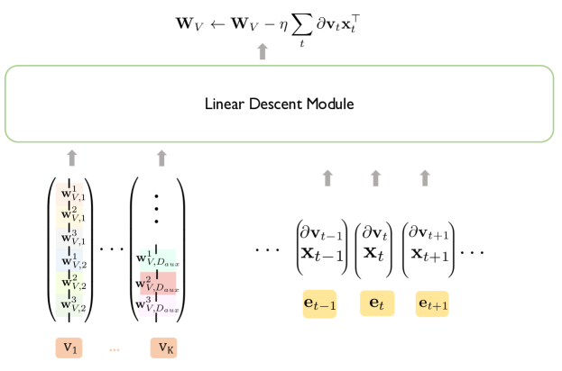
TinT can efficiently perform simulated gradient descent of an auxiliary model.
Theorem 1.1.
Consider an auxiliary transformer with layers, embedding dimension, attention heads, and a maximum sequence length of .
Given a hyperparameter (see Section 3.1), TinT can perform an efficient forward pass (Section 3), compute the simulated gradient (Section 4), and evaluate the updated auxiliary model with a total of
parameters, with constants .
The TinT model has embedding dimension and attention heads.
See Table 3 for a detailed breakdown of the parameters.
Large transformers (Vaswani et al., 2017) have brought about a revolution in language modeling, with scaling yielding significant advancements in capabilities (Brown et al., 2020; Chowdhery et al., 2022). These capabilities include performing in-context learning or following natural language instructions at inference time.
Researchers have tried to understand how these models can learn new tasks without parameter updates (Garg et al., 2022; von Oswald et al., 2023; Xie et al., 2022; Nanda et al., 2023). A popular hypothesis is that in-context learning corresponds to the transformer (referred to as the simulator from now on) simulating gradient-based learning of a smaller model (called auxiliary model) that is embedded within it.
From perspective of AI safety and alignment (Amodei et al., 2016; Leike et al., 2018; Askell et al., 2021), the ability of a larger model to use input data (which could be arbitrary in a deployed setting) to implicitly train an auxiliary model feels worrisome. This concern felt minor due to efficiency considerations: previous analyses and experiments required the auxiliary model to be quite tiny compared to the simulator. For instance, simulating and training an auxiliary model that is a linear layer requires tens of millions of parameters in the simulator (Akyurek et al., 2022). This scaling is even more dramatic if the auxiliary model is a multi-layer fully-connected net (Giannou et al., 2023).
Our primary contribution is an explicit and nontrivial construction of a simulator called TinT that explicitly adapts to the context without parameter updates. In particular, we show that a forward pass through a modestly sized TinT can involve gradient-based training of an auxiliary model that is itself a large transformer. For example, we show that TinT with 2B parameters can faithfully simulate fine-tuning a 125M parameter auxiliary transformer in a single forward pass. (Prior constructions would have required trillions of parameters in the simulator for a far simpler auxiliary model.)
Our main result is described in Theorem 1.1, which details how the size of TinT depends on the auxiliary model. Our construction is generally applicable to diverse variants of pre-trained language models. The rest of the paper is structured to highlight the key design choices and considerations in TinT.
-
1.
Section 2 discusses the overall design decisions required to make TinT, including how the simulator can read from and write to the auxiliary model and how the data must be formatted.
-
2.
Section 3 uses the linear layer as an example to describe how highly parallelized computation and careful rearrangement of activations enable TinT to efficiently simulate the forward pass of the auxiliary model.
-
3.
Section 4 describes how TinT uses first-order approximations and stop gradients to compute the simulated gradient of the auxiliary model.
-
4.
Section 5 performs experiments comparing TinT to suitable baselines in language modeling and in-context learning settings. Our findings validate that the simulated gradient can effectively update large pre-trained auxiliary models. Notably, we instantiate TinT in a highly extensible codebase, making TinT the first such construction to undergo end-to-end evaluation.
Due to the complexity of the construction, we defer the formal details of TinT to the appendix.
2 Design Considerations
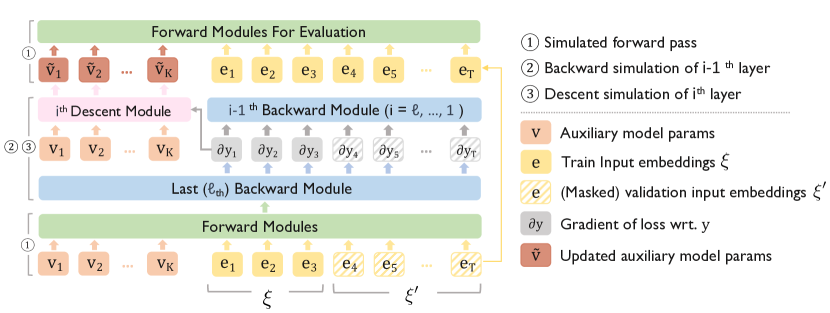
Our goal is to construct a simulator that can train an auxiliary model over the course of an inference pass. This procedure requires four steps:
-
1.
Forward Pass: A forward pass to compute the auxiliary model output on training input and a loss .
-
2.
Backward Pass: Backpropagation to compute the gradient of the auxiliary model .
-
3.
Parameter Update: Update the auxiliary model using gradient descent, setting .
-
4.
Output: Output next-token predictions on a test input using the updated auxiliary model.
Note that steps 1-3 can be looped to train the auxiliary model for a few steps222Looping steps 1-3 scales the depth of the simulator model., either on the same training data or on different training data for each step, before evaluating it on the test input (Giannou et al., 2023). The above method highlight two crucial features of the simulator: (1) it has access to some amount of training data, and (2) it can use (i.e., read) and update (i.e., write) the auxiliary model. Below, we discuss how to design a modest-sized simulator around these two considerations.
2.1 Input structure
For simplicity, we describe only one update step on a single batch of training data but note that our formal construction and our experiments handle multiple training steps (see Definition 5.1). Steps 1 and 4 show that the simulator must access some training data to train the auxiliary model and some testing data on which it evaluates the updated auxiliary model. For the sake of illustration we consider the following simple setting: given a sequence of input tokens , we split it into training data and testing data .
Suppose contains an in-context input-output exemplar and contains a test input. Then, the simulator performs a very natural operation of training the auxiliary model on a task-specific example and outputs results for the test example.
On the other hand, if the input is not specially formatted, and may simply contain some natural language tokens. In this case, the simulator is using the first part of the context tokens to do a quick fine-tune of the auxiliary for some task before outputting the subsequent tokens with the auxiliary model. In a worst-case scenario, users might provide harmful contents, leading the model to implicitly fine-tune on them and potentially output even more harmful content.
Our experiments consider many options for splitting a sequence into and , and we defer a more detailed discussion of possible setups to Section 5.
Accessing Training Labels.
The simulator must be able to see the labels of the training tokens in order to compute the loss (usually, the autoregressive cross-entropy loss) in step 1. For example, in Figure 1, when we compute the loss for the token in the second position, we need to use its label in the third position. However, this is not possible if the simulator uses strictly autoregressive attention (Appendix H contains a more general discussion). We thus use a bidirectional attention mask on the training tokens and autoregressive attention on the evaluation portion. We note that encoding relevant (e.g., retrieved) context with bidirectional attention is a popular way to improve autoregressive capabilities in language modeling and natural language tasks (Raffel et al., 2020; Borgeaud et al., 2022; Izacard & Grave, 2020; Izacard et al., 2023; Wang et al., 2023a; Tay et al., 2022). This empirical approach is similar in motivation to how TinT uses a few context tokens to adapt the auxiliary model to a given input. Having established the training and testing data, we can now move to discussing how the simulator can access (i.e., read) and update (i.e., write to) the auxiliary model at inference time.
2.2 Read and write access to auxiliary model
As discussed in the start of this section, the simulator must have read and write access to the parameters of the auxiliary model. Crucially, the simulator must do at least two forward passes through the auxiliary model, one with the current parameters and one with the updated parameters .
The straightforward way to simulate the forward pass of the auxiliary model would be to store its weights in the simulator’s weights and run a forward pass as usual. One can analogously simulate the backward pass according to the loss to compute the gradients. However, the simulator cannot update its own weights at inference time, so this strategy would not permit the model to write the updated parameters and later read them when simulating the second forward pass. Therefore, the auxiliary model must be available in the activations of the simulator.
To this end, Wei et al. (2021); Perez et al. (2021) model the simulator after a Turing machine, where the activation in each layer acts as a workspace for operations, and computation results are copied to and from memory using attention operations. In this paradigm, if , computing a dot product with weight requires at least million parameters in the simulator333 Using a feedforward module to mimic the dot product (as in Akyurek et al. (2022), see thm. C.4), where the simulator embedding comprises , necessitates a minimum of million parameters. Using an attention module to copy the weight from memory adds another million parameters.. Given the pervasiveness of dot products in neural network modules, this strategy would yield a simulator with trillions of parameters.
Alternatively, one can store parameters in the first few context tokens and allow the attention modules to attend to those tokens (Giannou et al., 2023). This removes the need for copying and token-wise operations. Then, the same dot product requires only a self-attention module with million parameters. We thus adopt this strategy to provide relevant auxiliary model weights as prefix embeddings.
Definition 2.1 (Prefix Embeddings).
denotes the prefix embeddings at the th layer in TinT. These contain relevant auxiliary model weights or simulated activations.
We now consider how to efficiently simulate the building block of neural networks: matrix-vector multiplication. In the next section, we demonstrate that a careful construction of the prefix embeddings enables efficient parallelizaton of matrix-vector products across attention heads.
3 Efficient Forward Propagation
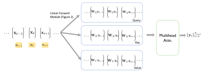
We now discuss how TinT performs a highly efficient forward pass through the auxiliary model. Here, we focus on the linear layer because it is repeated many times in various transformer modules (e.g., in self-attention), so improving the efficiency dramatically reduces TinT’s size.
Definition 3.1 (Linear layer).
For a weight , a linear layer takes as input and outputs .444Linear layers are applied token-wise, so we can consider a single position without loss of generality.
We compute coordinate-wise, i.e., for all , where is the th row of . The simulator represents as an attention score between the row and the input . So, the input embeddings contain in the first coordinates, and the rows of the weight matrix are in prefix embeddings (def. 2.1).
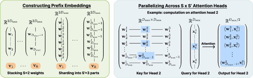
We strategically distribute the weights (§3.1) and aggregate the parallelized computation results (§3.2). As we briefly mentioned in the previous section, a straightforward construction of the linear layer would use the context and attention heads inefficiently. Our construction instead parallelizes the computation across attention heads in such a way that aggregating the output of the linear operation can also be conducted efficiently.
3.1 Stacking and Sharding
We partition the inner product computation across attention heads by carefully rearranging the weights and activations via stacking and sharding (Figure 2).
Instead of representing each weight as its own prefix token , we stack weights on top of each other to form each prefix embedding . drives a trade-off between the embedding dimension of the TinT, , and the context length to the TinT, . We set .
A simple strategy now would be to use different attention heads to operate on different rows; however, this would still use only attention heads whereas we could parallelize across many more heads. We instead parallelize across more attention heads, where each head is responsible for computing the inner product on a subset of the coordinates. We shard each individual weight and the activation into parts and compute the inner product on each of the parts in parallel We set and such that , thereby using all of TinT heads to efficiently compute the dot products.
3.2 Efficient Aggregation
The attention module outputs a sparse matrix with shape containing the inner products on various subsets of the coordinates in its entries. To complete the linear forward pass, we need to sum the appropriate terms to form a -length vector with in the first coordinates. Straightforwardly summing along an axis aggregates incorrect terms, since the model was sharded. On the other hand, rearranging the matrix would require an additional linear layer. Instead, TinT saves a factor of parameters by leveraging the local structure of the attention output. We illustrate this visually in Section D.1. This procedure requires parameters. This efficient aggregation also compresses the constructions for the TinT’s backpropagation modules for layer normalization and activations (Appendices F and G).
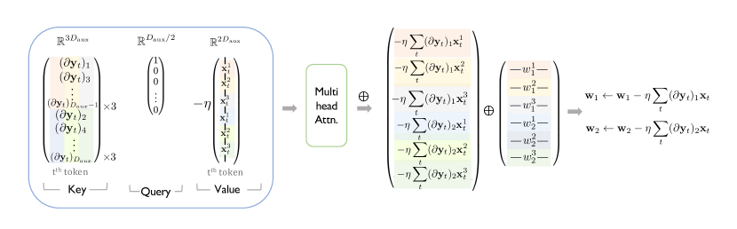
4 Simulated Gradient
TinT adapts backpropagation to compute gradients (Figure 1). We aim to train a capable (i.e., pre-trained) auxiliary model for just a few steps, so high precision gradients may be unnecessary. Instead, TinT performs an approximate backpropagation. TinT then uses this simulated gradient to update the auxiliary model. Prior works computed similar approximate gradients in hopes of more faithfully modeling neurobiology (Scellier & Bengio, 2017; Hinton, 2022) or improving the efficiency of training models (Hu et al., 2021; Malladi et al., 2023). We note that the approximations in the simulated gradients can be made stronger at the cost of enlarging TinT. Indeed, one could construct a simulator to exactly perform the procedure outlined in §2, though it would be orders of magnitude larger than TinT. For brevity’s sake, we focus on the key approximations and design choices and defer formal details to the appendix.
4.1 First-order approximations
We use first-order approximations of gradients to backpropagate through the layer normalization layer.555We discuss a layer normalization layer without scale and bias parameters, but Appendix F contains a general construction. It normalizes the input using its mean and standard deviation across the input dimensions. Since the operation is token-wise, we can consider a single position without loss of generality.
Definition 4.1 (Layer normalization).
A layer normalization layer takes input and outputs , where and denote its mean and standard deviation.
High precision gradients: Formally, for input-output pair , we can compute the gradients , with chain rule:
| (1) |
Inefficiency of exact computation: A TinT layer simulating backpropagation through an auxiliary’s layer normalization layer receives and in its input embeddings. We go through the exact gradient and why it is inefficient.
For exact computation one could first compute using a normalization layer and store in the embeddings. However, inefficiency arises from computing the term . To calculate at each token position , we could either: (1) use a two-layer MLP that focuses on each token separately, or (2) a single self-attention module to treat the operation as a sequence-to-sequence task.
For (1) we could initially compute via an MLP, followed by computation of using another MLP. The element-wise multiplication in embeddings would be facilitated with a nonlinear activation function like GeLU (Akyurek et al., 2022) (refer to thm. C.4 for details). However, this approach would need substantial number of simulator parameters to represent the MLPs.
Alternatively, we could use a single self-attention module. Constructing such a module would require careful engineering to make sure the input tokens only attend to themselves while keeping an attention score of to others. If we used a linear attention, we would need to space out the gradient and in each position , such that the attention score is between different tokens. This would require an embedding dimension proportional to the context length. On the other hand, if we used a softmax attention module, we would need an additional superfluous token in the sequence. Then, a token at position would attend to itself with attention and to the extra token with an attention score of . The extra token would return a value vector . To avoid such inefficiency, we opt for a first-order approximation instead.
Efficient approximation: Instead of explicitly computing each term in the chain rule of in Eq. 1, we instead use a first order Taylor expansion of .
Rearranging allows us to write
Similar to the computation of Eq. 1, we can show
Because is symmetric666For a linear function with matrix , . Since may not be a symmetric matrix, this method can’t be generally applied to approximately backpropagate linear layers or causal self-attention layers., we can write
Then, ignoring the small error term, we can use just two linear layers, separated by a normalization layer, to simulate the approximation.
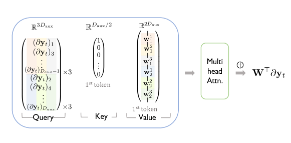
4.2 Fuzzy backpropagation via stop gradients
Self-attention is inherently quadratic, because it uses the keys and queries to compute attention scores between every possible pair of tokens in the sequence. These scores then linearly combine the value vectors (see def. B.1). Computing the gradient exactly is thus a very complex operation. Instead, we stop the gradient computation through attention scores in the self-attention layer. For similar reasons, we only update the value parameter in the self-attention module.
Gradient backpropagation: For an input, output sequence pair , if denote the intermediate query, key, value vectors, on gradients , is given via the chain rule:
| (2) |
Here, denote the query, key, and value matrices.
Inefficiency in exact computation: Here, we demonstrate that simulating computation of the three terms in Eq. 2 is inefficient, because depend on the derivatives w.r.t. the attention scores. As an example, we focus on :
Computing this term would require us at least 2 self-attention layers and an MLP layer. The first attention layer would compute for different token pairs, similar to the forward simulation of a linear layer with linear attention (§3). These would be then multiplied to the pair-wise attention scores with an MLP to compute , with elementwise product would be facilitated by GeLU non-linearity (thm. C.4). These would be finally used by an attention layer to combine the different key vectors. A similar simulation would be necessary to compute .
Stop gradients through query and key vectors: In order to reduce the necessary resources, we ignore the query and key gradients in Eq. 2. When we ignore these gradient components, can be simplified as
| (3) |
A single self-attention layer can compute this by using the attention scores to combine the token-wise gradients.
Why won’t it hurt performance? Estimating as described is motivated by recent work (Malladi et al., 2023) showing that fuzzy gradient estimates don’t adversely affect fine-tuning of pre-trained models. Furthermore, we theoretically show that when the attention head for each position pays a lot of attention to a single token (i.e., behaves like hard attention (Perez et al., 2021)), the approximate gradient in Eq. 3 is entry-wise close to the true gradients (thm. E.5).
The other approximation is to update only the value parameters of the auxiliary model (§E). This is motivated by parameter efficient fine-tuning methods like LoRA (Hu et al., 2021) and IA3 (Liu et al., 2022), which restrict the expressivity of the gradient updates without degrading the quality of the resulting model. We similarly show in the next section that the simulated gradients in TinT can effectively tune large pre-trained transformers.
| Training proportion | |||||
| Evaluating with | |||||
| GPT-2 | Auxiliary Model | 25.6 | 24.9 | 24.5 | 23.3 |
| Fine-tuning | 24.9 | 24.0 | 23.5 | 22.2 | |
| TinT | 25.1 | 24.3 | 23.8 | 22.6 | |
| OPT-125M | Auxiliary Model | 29.6 | 28.8 | 28.0 | 28.0 |
| Fine-tuning | 29.0 | 28.2 | 27.4 | 27.4 | |
| TinT | 29.3 | 28.4 | 27.5 | 27.4 | |
5 Experiments
| Model | Shots | Subj | AGNews | SST2 | CR | MR | MPQA | Amazon | Avg. |
| OPT-125m | |||||||||
| OPT-1.3b | |||||||||
| OPT-125m Fine-tuning | |||||||||
| OPT-125m TinT | |||||||||
| OPT-125m | |||||||||
| OPT-1.3b | |||||||||
| OPT-125m Fine-tuning | |||||||||
| OPT-125m TinT |
We evaluate the performance of the TinTs constructed using GPT2 and OPT-125M as auxiliary models. The findings from our experiments in the language modeling and in-context learning settings confirm that fine-tuning with the simulated gradients (Section 4) still allows for effective learning in the auxiliary model. We loop the training steps (i.e., steps 1-3) outlined in Section 2 to accommodate solving real-world natural language tasks. We formalize the setting below.
5.1 Setting: -step Fine-Tuning
We formalize the procedure in Section 2 to construct a suitable setting in which we can compare TinT to explicitly training the auxiliary model.
Definition 5.1 (-step Fine-Tuning).
Given a batch of training datapoints and a validation input , we compute and apply gradient updates on the auxiliary model for timesteps as
where is the learning rate and is a self-supervised loss function on each input . Then, we evaluate the model on . denotes the pre-trained auxiliary model.
Below, we instantiate this setting with text inputs of different formats and different self-supervised loss functions . To manage computational demands, we limit to or fewer.777Performing many gradient steps scales the depth of TinT and makes experimentation computationally infeasible.
5.2 Case Study: Language Modeling
The first case we consider is language modeling, where the input data is natural language without any additional formatting. We use a batch size of in def. 5.1, and delegate and . The loss is the sum of the token-wise autoregressive cross-entropy loss in the sequence . For example, given an input Machine learning is a useful tool for solving problems., we use the red part as the training data , and the brown part as the validation data . We perform language modeling experiments on WikiText-103 (Merity et al., 2016) and vary the number of tokens used as training data .
Results. In Table 1, we observe that TinT achieves a performance comparable to explicit fine-tuning of the auxiliary model, indicating that the simulated gradient (Section 4) is largely effective for fine-tuning. Both TinT and explicitly fine-tuning the auxiliary model show improvement over the base model, confirming that minimal tuning on the context indeed enhances predictions on the test portion.
5.3 Case Study: In-Context Learning
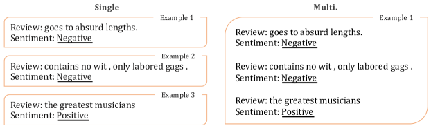
For in-context learning, we consider input data to be a supervised classification task transformed into a next-token prediction task using surrogate labels (see Figure 3). Using binary sentiment classification of movie reviews as an example, given an input (e.g., the review), the model’s predicted label is computed as follows. First, we design a simple task-specific prompt (e.g., “Sentiment:”) and select label words to serve as surrogates for each class (e.g., “positive” and “negative”). Then, we provide the input along with the prompt to the model, and the label assigned the highest probability is treated as the model’s prediction. We describe the zero-shot and few-shot settings below.
Zero-shot. In the zero-shot setting, we are given text with the first tokens as the input text and final token as the surrogate text label. Hence, we adapt def. 5.1 to use batch size , training data , and testing data . The loss is again the sum of the token-wise autoregressive cross-entropy losses.
Few-shot. In the few-shot setting, we are given input texts that are a concatenation of sequences . Each sequence contains the input text followed by the surrogate label for the in-context exemplar. These exemplars are followed by test data . In this case, we can compute the gradient updates to in two different ways (Figure 3). The first setting, denoted Single, treats the sequences as a batch of training datapoints . The second setting, denoted Multi, treats the concatenation of the sequences as a single training datapoint . Furthermore, for a training datapoint can be defined in two different ways. The first setting, denoted as Full context loss, defines for a training datapoint as the sum of cross entropy loss over all tokens. The second setting, denoted as Label loss, defines for a training datapoint in def. 5.1 as the sum of cross entropy loss over the surrogate label tokens.
Tasks. We evaluate 7 classification tasks for zero-shot and few-shot settings: SST-2 (Socher et al., 2013), MR (Pang & Lee, 2004), CR (Hu & Liu, 2004), MPQA (Wiebe et al., 2005), Amazon Polarity (Zhang et al., 2015), AGNews (Zhang et al., 2015), and Subj (Pang & Lee, 2005).
Model. We compare a TinT model that uses an OPT-125m pre-trained model as its auxiliary model against two alternative approaches: (1) directly fine-tuning OPT-125m, and (2) performing standard evaluation using OPT-1.3b, which is of a similar size to TinT.888Our construction is generally applicable to diverse variants of pre-trained language models (Appendix K).
Observations. We observe that inferences passes through TinT perform on par with directly fine-tuning the auxiliary model, affirming the validity of the construction design (see Section 2). As expected, TinT outperforms the base auxiliary model, since it simulates training the auxiliary model. More intriguingly, TinT demonstrates performance comparable to a pre-trained model of similar size (OPT-1.3b). This suggests that the capabilities of existing pre-trained models may be understood via the simulation of smaller auxiliary models. For further details and results of the experiments, please refer to Appendix L.
6 Related Work
Gradient-based learning and in-context learning: Several works relate in-context learning to gradient-based learning algorithms. Bai et al. (2023) explicitly constructed transformers to simulate simple gradient-based learning algorithms. Mahankali et al. (2023); Ahn et al. (2023) suggested one attention layer mimics gradient descent on a linear layer, and Zhang et al. (2023a) showed polynomial convergence. Cheng et al. (2023); Han et al. (2023) extended these ideas to non-linear attentions. Experiments in Dai et al. (2022) suggest that LLM activations during in-context learning mirror fine-tuned models. These works focus on using a standard transformer for the simulator and hence cannot accommodate more complex auxiliary models; on the other hand, our work uses structural modifications and approximations to construct an efficient simulator for complex auxiliary models. Our work in contrast attempts to build even stronger transformers by introducing few structural modifications that can run gradient descent on auxiliary transformers.
Transformer Expressivity: Perez et al. (2021); Pérez et al. (2019) show that Transformers with hard attention are Turing complete, and Wei et al. (2021) construct transformers to study statistical learnability, but the proposed constructions are extremely large. Other works have investigated encoding specific algorithms in smaller simulators, e.g. bounded-depth Dyck languages (Yao et al., 2021), modular prefix sums (Anil et al., 2022), adders (Nanda et al., 2023), regular languages (Bhattamishra et al., 2020), and sparse logical predicates (Edelman et al., 2022). Liu et al. (2023) aim to understand automata-like mechanisms within transformers. Ba et al. (2016) connect self-attention and fast weight programmers (FWPs), which compute input-dependent weight updates during inference. Follow-up works (Schlag et al., 2021; Irie et al., 2021) use self-attention layers to update linear and recurrent networks during inference. Clark et al. (2022) add and efficiently tune Fast Weights Layers (FWL) on a frozen pre-trained model.
7 Discussion
We present a parameter-efficient construction TinT capable of simulating gradient descent on an internal transformer model during inference. Using fewer than 2 billion parameters, it can simulate fine-tuning a 125 million transformer (e.g., GPT-2) internally, dramatically reducing the scale required by previous works. Language modeling and in-context learning experiments demonstrate that the efficient approximations still allow the TinT to fine-tune the model. Our work emphasizes that the inference behavior of complex models may rely on the training dynamics of smaller models. As such, the existence of TinT has strong implications for interpretability and AI alignment research.
While our work represents a significant improvement over previous simulations in terms of auxiliary model complexity, similar to prior research in this area, our insights into existing pre-trained models are limited. Furthermore, we have not yet examined potential biases that may arise in the auxiliary models due to one-step gradient descent. We plan to investigate these aspects in future work.
Impact Statements
We note that the construction of TinT does not appear to increase the probability of harmful behavior, because the construction’s primary objective is to implicitly tune an internal model (§2). Such tuning has been possible for a long time and is not made more expressive by TinT.
Our findings suggest that existing transformer-based language models can plausibly possess the ability to learn and adapt to context by internally fine-tuning a complex model even during inference. Consequently, although users are unable to directly modify deployed models, these models may still undergo dynamic updates while processing a context left-to-right, resulting in previously unseen behavior by the time the model reaches the end of the context. This has significant implications for the field of model alignment. It is challenging to impose restrictions on a model that can perform such dynamics updates internally, so malicious content can influence the output of deployed models.
Alternatively, we recognize the potential benefits of pre-training constructed models that integrate explicit fine-tuning mechanisms. By embedding the functionalities typically achieved through explicit fine-tuning, such as detecting malicious content and intent within the models themselves, the need for external modules can be mitigated. Pre-training the constructed model may offer a self-contained solution for ensuring safe and responsible language processing without relying on external dependencies.
Acknowledgements
The authors acknowledge funding from NSF, ONR, Simons Foundation, and DARPA. We thank Danqi Chen, Jason Lee, Zhiyuan Li, Kaifeng Lyu, Simran Kaur, Tianyu Gao, and Colin Wang for their suggestions and helpful discussions at different stages of our work.
References
- Ahn et al. (2023) Ahn, K., Cheng, X., Daneshmand, H., and Sra, S. Transformers learn to implement preconditioned gradient descent for in-context learning. arXiv preprint arXiv:2306.00297, 2023.
- Akyurek et al. (2022) Akyurek, E., Schuurmans, D., Andreas, J., Ma, T., and Zhou, D. What learning algorithm is in-context learning? investigations with linear models. arXiv preprint arXiv:2211.15661, 2022.
- Amodei et al. (2016) Amodei, D., Olah, C., Steinhardt, J., Christiano, P., Schulman, J., and Mané, D. Concrete problems in ai safety. arXiv preprint arXiv:1606.06565, 2016.
- Anil et al. (2022) Anil, C., Wu, Y., Andreassen, A., Lewkowycz, A., Misra, V., Ramasesh, V., Slone, A., Gur-Ari, G., Dyer, E., and Neyshabur, B. Exploring length generalization in large language models. arXiv preprint arXiv:2207.04901, 2022.
- Askell et al. (2021) Askell, A., Bai, Y., Chen, A., Drain, D., Ganguli, D., Henighan, T., Jones, A., Joseph, N., Mann, B., DasSarma, N., et al. A general language assistant as a laboratory for alignment. arXiv preprint arXiv:2112.00861, 2021.
- Ba et al. (2016) Ba, J., Hinton, G., Mnih, V., Leibo, J. Z., and Ionescu, C. Using fast weights to attend to the recent past, 2016.
- Bai et al. (2023) Bai, Y., Chen, F., Wang, H., Xiong, C., and Mei, S. Transformers as statisticians: Provable in-context learning with in-context algorithm selection. arXiv preprint arXiv:2306.04637, 2023.
- Bhattamishra et al. (2020) Bhattamishra, S., Ahuja, K., and Goyal, N. On the ability and limitations of transformers to recognize formal languages. arXiv preprint arXiv:2009.11264, 2020.
- Borgeaud et al. (2022) Borgeaud, S., Mensch, A., Hoffmann, J., Cai, T., Rutherford, E., Millican, K., Van Den Driessche, G. B., Lespiau, J.-B., Damoc, B., Clark, A., et al. Improving language models by retrieving from trillions of tokens. In International conference on machine learning, pp. 2206–2240. PMLR, 2022.
- Brown et al. (2020) Brown, T., Mann, B., Ryder, N., Subbiah, M., Kaplan, J. D., Dhariwal, P., Neelakantan, A., Shyam, P., Sastry, G., Askell, A., et al. Language models are few-shot learners. Advances in neural information processing systems, 33:1877–1901, 2020.
- Chan et al. (2022) Chan, S., Santoro, A., Lampinen, A., Wang, J., Singh, A., Richemond, P., McClelland, J., and Hill, F. Data distributional properties drive emergent in-context learning in transformers. Advances in Neural Information Processing Systems, 35:18878–18891, 2022.
- Cheng et al. (2023) Cheng, X., Chen, Y., and Sra, S. Transformers implement functional gradient descent to learn non-linear functions in context. arXiv preprint arXiv:2312.06528, 2023.
- Chowdhery et al. (2022) Chowdhery, A., Narang, S., Devlin, J., Bosma, M., Mishra, G., Roberts, A., Barham, P., Chung, H. W., Sutton, C., Gehrmann, S., et al. Palm: Scaling language modeling with pathways. arXiv preprint arXiv:2204.02311, 2022.
- Chughtai et al. (2023) Chughtai, B., Chan, L., and Nanda, N. A toy model of universality: Reverse engineering how networks learn group operations. arXiv preprint arXiv:2302.03025, 2023.
- Clark et al. (2022) Clark, K., Guu, K., Chang, M.-W., Pasupat, P., Hinton, G., and Norouzi, M. Meta-learning fast weight language models. In Proceedings of the 2022 Conference on Empirical Methods in Natural Language Processing, pp. 9751–9757, Abu Dhabi, United Arab Emirates, December 2022. Association for Computational Linguistics. URL https://aclanthology.org/2022.emnlp-main.661.
- Conmy et al. (2023) Conmy, A., Mavor-Parker, A. N., Lynch, A., Heimersheim, S., and Garriga-Alonso, A. Towards automated circuit discovery for mechanistic interpretability. arXiv preprint arXiv:2304.14997, 2023.
- Dai et al. (2022) Dai, D., Sun, Y., Dong, L., Hao, Y., Sui, Z., and Wei, F. Why can gpt learn in-context? language models secretly perform gradient descent as meta-optimizers, 2022.
- Edelman et al. (2022) Edelman, B. L., Goel, S., Kakade, S., and Zhang, C. Inductive biases and variable creation in self-attention mechanisms. In International Conference on Machine Learning, pp. 5793–5831. PMLR, 2022.
- Elhage et al. (2021) Elhage, N., Nanda, N., Olsson, C., Henighan, T., Joseph, N., Mann, B., Askell, A., Bai, Y., Chen, A., Conerly, T., et al. A mathematical framework for transformer circuits. Transformer Circuits Thread, 2021.
- Garg et al. (2022) Garg, S., Tsipras, D., Liang, P. S., and Valiant, G. What can transformers learn in-context? a case study of simple function classes. Advances in Neural Information Processing Systems, 35:30583–30598, 2022.
- Giannou et al. (2023) Giannou, A., Rajput, S., yong Sohn, J., Lee, K., Lee, J. D., and Papailiopoulos, D. Looped transformers as programmable computers, 2023.
- Gong et al. (2019) Gong, L., He, D., Li, Z., Qin, T., Wang, L., and Liu, T. Efficient training of bert by progressively stacking. In International conference on machine learning, pp. 2337–2346. PMLR, 2019.
- Hahn & Goyal (2023) Hahn, M. and Goyal, N. A theory of emergent in-context learning as implicit structure induction. arXiv preprint arXiv:2303.07971, 2023.
- Han et al. (2023) Han, C., Wang, Z., Zhao, H., and Ji, H. In-context learning of large language models explained as kernel regression. arXiv preprint arXiv:2305.12766, 2023.
- Hendrycks & Gimpel (2016) Hendrycks, D. and Gimpel, K. Gaussian error linear units (gelus). arXiv preprint arXiv:1606.08415, 2016.
- Hinton (2022) Hinton, G. The forward-forward algorithm: Some preliminary investigations, 2022.
- Holtzman et al. (2021) Holtzman, A., West, P., Shwartz, V., Choi, Y., and Zettlemoyer, L. Surface form competition: Why the highest probability answer isn’t always right. arXiv preprint arXiv:2104.08315, 2021.
- Hu et al. (2021) Hu, E. J., Shen, Y., Wallis, P., Allen-Zhu, Z., Li, Y., Wang, S., Wang, L., and Chen, W. Lora: Low-rank adaptation of large language models. arXiv preprint arXiv:2106.09685, 2021.
- Hu & Liu (2004) Hu, M. and Liu, B. Mining and summarizing customer reviews. In Proceedings of the tenth ACM SIGKDD international conference on Knowledge discovery and data mining, pp. 168–177, 2004.
- Irie et al. (2021) Irie, K., Schlag, I., Csordás, R., and Schmidhuber, J. Going beyond linear transformers with recurrent fast weight programmers. In Beygelzimer, A., Dauphin, Y., Liang, P., and Vaughan, J. W. (eds.), Advances in Neural Information Processing Systems, 2021. URL https://openreview.net/forum?id=ot2ORiBqTa1.
- Izacard & Grave (2020) Izacard, G. and Grave, E. Leveraging passage retrieval with generative models for open domain question answering. arXiv preprint arXiv:2007.01282, 2020.
- Izacard et al. (2023) Izacard, G., Lewis, P., Lomeli, M., Hosseini, L., Petroni, F., Schick, T., Dwivedi-Yu, J., Joulin, A., Riedel, S., and Grave, E. Atlas: Few-shot learning with retrieval augmented language models. Journal of Machine Learning Research, 24(251):1–43, 2023. URL http://jmlr.org/papers/v24/23-0037.html.
- Jiang (2023) Jiang, H. A latent space theory for emergent abilities in large language models. arXiv preprint arXiv:2304.09960, 2023.
- Kumar et al. (2022) Kumar, A., Shen, R., Bubeck, S., and Gunasekar, S. How to fine-tune vision models with sgd, 2022.
- Leike et al. (2018) Leike, J., Krueger, D., Everitt, T., Martic, M., Maini, V., and Legg, S. Scalable agent alignment via reward modeling: a research direction. arXiv preprint arXiv:1811.07871, 2018.
- Lindner et al. (2023) Lindner, D., Kramár, J., Rahtz, M., McGrath, T., and Mikulik, V. Tracr: Compiled transformers as a laboratory for interpretability. arXiv preprint arXiv:2301.05062, 2023.
- Liu et al. (2023) Liu, B., Ash, J. T., Goel, S., Krishnamurthy, A., and Zhang, C. Transformers learn shortcuts to automata. In The Eleventh International Conference on Learning Representations, 2023. URL https://openreview.net/forum?id=De4FYqjFueZ.
- Liu et al. (2022) Liu, H., Tam, D., Muqeeth, M., Mohta, J., Huang, T., Bansal, M., and Raffel, C. A. Few-shot parameter-efficient fine-tuning is better and cheaper than in-context learning. Advances in Neural Information Processing Systems, 35:1950–1965, 2022.
- Mahankali et al. (2023) Mahankali, A., Hashimoto, T. B., and Ma, T. One step of gradient descent is provably the optimal in-context learner with one layer of linear self-attention. arXiv preprint arXiv:2307.03576, 2023.
- Malladi et al. (2023) Malladi, S., Gao, T., Nichani, E., Damian, A., Lee, J. D., Chen, D., and Arora, S. Fine-tuning language models with just forward passes. In Thirty-seventh Conference on Neural Information Processing Systems, 2023. URL https://openreview.net/forum?id=Vota6rFhBQ.
- Merity et al. (2016) Merity, S., Xiong, C., Bradbury, J., and Socher, R. Pointer sentinel mixture models. arXiv preprint arXiv:1609.07843, 2016.
- Nanda et al. (2023) Nanda, N., Chan, L., Lieberum, T., Smith, J., and Steinhardt, J. Progress measures for grokking via mechanistic interpretability. arXiv preprint arXiv:2301.05217, 2023.
- Olsson et al. (2022) Olsson, C., Elhage, N., Nanda, N., Joseph, N., DasSarma, N., Henighan, T., Mann, B., Askell, A., Bai, Y., Chen, A., et al. In-context learning and induction heads. arXiv preprint arXiv:2209.11895, 2022.
- Pang & Lee (2004) Pang, B. and Lee, L. A sentimental education: Sentiment analysis using subjectivity summarization based on minimum cuts. In Proceedings of the 42nd Annual Meeting of the Association for Computational Linguistics (ACL-04), pp. 271–278, 2004.
- Pang & Lee (2005) Pang, B. and Lee, L. Seeing stars: Exploiting class relationships for sentiment categorization with respect to rating scales. In Proceedings of the 43rd Annual Meeting of the Association for Computational Linguistics (ACL’05), pp. 115–124, 2005.
- Perez et al. (2021) Perez, J., Barcelo, P., and Marinkovic, J. Attention is turing-complete. Journal of Machine Learning Research, 22(75):1–35, 2021. URL http://jmlr.org/papers/v22/20-302.html.
- Press et al. (2021) Press, O., Smith, N. A., and Lewis, M. Train short, test long: Attention with linear biases enables input length extrapolation. arXiv preprint arXiv:2108.12409, 2021.
- Pérez et al. (2019) Pérez, J., Marinković, J., and Barceló, P. On the turing completeness of modern neural network architectures. In International Conference on Learning Representations, 2019. URL https://openreview.net/forum?id=HyGBdo0qFm.
- Raffel et al. (2020) Raffel, C., Shazeer, N., Roberts, A., Lee, K., Narang, S., Matena, M., Zhou, Y., Li, W., and Liu, P. J. Exploring the limits of transfer learning with a unified text-to-text transformer. The Journal of Machine Learning Research, 21(1):5485–5551, 2020.
- Reddi et al. (2023) Reddi, S. J., Miryoosefi, S., Karp, S., Krishnan, S., Kale, S., Kim, S., and Kumar, S. Efficient training of language models using few-shot learning. 2023.
- Saunshi et al. (2020) Saunshi, N., Malladi, S., and Arora, S. A mathematical exploration of why language models help solve downstream tasks. arXiv preprint arXiv:2010.03648, 2020.
- Scao et al. (2022) Scao, T. L., Fan, A., Akiki, C., Pavlick, E., Ilić, S., Hesslow, D., Castagné, R., Luccioni, A. S., Yvon, F., Gallé, M., et al. Bloom: A 176b-parameter open-access multilingual language model. arXiv preprint arXiv:2211.05100, 2022.
- Scellier & Bengio (2017) Scellier, B. and Bengio, Y. Equilibrium propagation: Bridging the gap between energy-based models and backpropagation. Frontiers in computational neuroscience, 11:24, 2017.
- Schlag et al. (2021) Schlag, I., Irie, K., and Schmidhuber, J. Linear transformers are secretly fast weight memory systems. CoRR, abs/2102.11174, 2021. URL https://arxiv.org/abs/2102.11174.
- Shazeer (2020) Shazeer, N. Glu variants improve transformer. arXiv preprint arXiv:2002.05202, 2020.
- Socher et al. (2013) Socher, R., Perelygin, A., Wu, J., Chuang, J., Manning, C. D., Ng, A. Y., and Potts, C. Recursive deep models for semantic compositionality over a sentiment treebank. In Proceedings of the 2013 conference on empirical methods in natural language processing, pp. 1631–1642, 2013.
- Su et al. (2021) Su, J., Lu, Y., Pan, S., Murtadha, A., Wen, B., and Liu, Y. Roformer: Enhanced transformer with rotary position embedding. arXiv preprint arXiv:2104.09864, 2021.
- Tay et al. (2022) Tay, Y., Dehghani, M., Tran, V. Q., Garcia, X., Wei, J., Wang, X., Chung, H. W., Bahri, D., Schuster, T., Zheng, S., et al. Ul2: Unifying language learning paradigms. In The Eleventh International Conference on Learning Representations, 2022.
- Touvron et al. (2023) Touvron, H., Lavril, T., Izacard, G., Martinet, X., Lachaux, M.-A., Lacroix, T., Rozière, B., Goyal, N., Hambro, E., Azhar, F., et al. Llama: Open and efficient foundation language models. arXiv preprint arXiv:2302.13971, 2023.
- Vaswani et al. (2017) Vaswani, A., Shazeer, N., Parmar, N., Uszkoreit, J., Jones, L., Gomez, A. N., Kaiser, Ł., and Polosukhin, I. Attention is all you need. Advances in neural information processing systems, 30, 2017.
- von Oswald et al. (2023) von Oswald, J., Niklasson, E., Schlegel, M., Kobayashi, S., Zucchet, N., Scherrer, N., Miller, N., Sandler, M., Vladymyrov, M., Pascanu, R., et al. Uncovering mesa-optimization algorithms in transformers. arXiv preprint arXiv:2309.05858, 2023.
- Wang et al. (2023a) Wang, B., Ping, W., Xu, P., McAfee, L., Liu, Z., Shoeybi, M., Dong, Y., Kuchaiev, O., Li, B., Xiao, C., Anandkumar, A., and Catanzaro, B. Shall we pretrain autoregressive language models with retrieval? a comprehensive study. In Bouamor, H., Pino, J., and Bali, K. (eds.), Proceedings of the 2023 Conference on Empirical Methods in Natural Language Processing, pp. 7763–7786, Singapore, December 2023a. Association for Computational Linguistics. doi: 10.18653/v1/2023.emnlp-main.482. URL https://aclanthology.org/2023.emnlp-main.482.
- Wang et al. (2022) Wang, K. R., Variengien, A., Conmy, A., Shlegeris, B., and Steinhardt, J. Interpretability in the wild: a circuit for indirect object identification in GPT-2 small. In NeurIPS ML Safety Workshop, 2022. URL https://openreview.net/forum?id=rvi3Wa768B-.
- Wang et al. (2023b) Wang, X., Zhu, W., and Wang, W. Y. Large language models are implicitly topic models: Explaining and finding good demonstrations for in-context learning. arXiv preprint arXiv:2301.11916, 2023b.
- Wei et al. (2021) Wei, C., Chen, Y., and Ma, T. Statistically meaningful approximation: a case study on approximating turing machines with transformers. CoRR, abs/2107.13163, 2021. URL https://arxiv.org/abs/2107.13163.
- Weiss et al. (2021) Weiss, G., Goldberg, Y., and Yahav, E. Thinking like transformers. In International Conference on Machine Learning, pp. 11080–11090. PMLR, 2021.
- Wiebe et al. (2005) Wiebe, J., Wilson, T., and Cardie, C. Annotating expressions of opinions and emotions in language. Language resources and evaluation, 39:165–210, 2005.
- Wies et al. (2023) Wies, N., Levine, Y., and Shashua, A. The learnability of in-context learning. arXiv preprint arXiv:2303.07895, 2023.
- Xie et al. (2022) Xie, S. M., Raghunathan, A., Liang, P., and Ma, T. An explanation of in-context learning as implicit bayesian inference. In International Conference on Learning Representations, 2022. URL https://openreview.net/forum?id=RdJVFCHjUMI.
- Yao et al. (2021) Yao, S., Peng, B., Papadimitriou, C., and Narasimhan, K. Self-attention networks can process bounded hierarchical languages. arXiv preprint arXiv:2105.11115, 2021.
- Zhang & Sennrich (2019) Zhang, B. and Sennrich, R. Root mean square layer normalization. Advances in Neural Information Processing Systems, 32, 2019.
- Zhang et al. (2023a) Zhang, R., Frei, S., and Bartlett, P. L. Trained transformers learn linear models in-context. arXiv preprint arXiv:2306.09927, 2023a.
- Zhang et al. (2015) Zhang, X., Zhao, J., and LeCun, Y. Character-level convolutional networks for text classification. Advances in neural information processing systems, 28, 2015.
- Zhang et al. (2023b) Zhang, Y., Zhang, F., Yang, Z., and Wang, Z. What and how does in-context learning learn? bayesian model averaging, parameterization, and generalization. arXiv preprint arXiv:2305.19420, 2023b.
- Zhou et al. (2023) Zhou, H., Bradley, A., Littwin, E., Razin, N., Saremi, O., Susskind, J., Bengio, S., and Nakkiran, P. What algorithms can transformers learn? a study in length generalization. arXiv preprint arXiv:2310.16028, 2023.
Brief overview of the appendix
In Appendix A, we report few additional related works. In Appendix B, we present some of the deferred definitions from the main paper. In Appendix C, we present all the important notations used to present the design of TinT. In Appendices D, E, F and G, we present the simulation details of all operations on linear, self-attention, layer normalization, and activation layers respectively for an auxiliary model. In Appendix H, we present the details for simulating loss computation with the language model head of the auxiliary model. In Appendix J, we discuss simulation of additional modules necessary to simulate transformer variants like LLaMA (Touvron et al., 2023) and BLOOM (Scao et al., 2022). Finally, in Appendix L, we discuss the deferred experimental details from the main paper.
Appendix A Additional related works
Interpretability: Mechanistic interpretability works reverse-engineer the algorithms simulated by these models (Elhage et al., 2021; Olsson et al., 2022; Wang et al., 2022; Nanda et al., 2023; Chughtai et al., 2023; Conmy et al., 2023). These works study local patterns, e.g. activations and attention heads, to derive interpretable insights. Other works (Weiss et al., 2021; Lindner et al., 2023) use declarative programs to algorithmically describe transformer models. Zhou et al. (2023) use these to explain task-specific length generalization of transformer models.
Alternative Explanations for ICL: Some works study ICL using a Bayesian framework. Xie et al. (2022) model pretraining data as a mixture of HMMs and cast ICL identifying one such component. Hahn & Goyal (2023) later modeled language as a compositional grammar, and propose ICL as a composition of operations. (Zhang et al., 2023b; Jiang, 2023; Wang et al., 2023b; Wies et al., 2023) further strengthen this hypothesis by generalizing the underlying latent space. On the other hand, careful experiments in Chan et al. (2022) show that data distributional properties (e.g. Zipf’s law) drive in-context learning in transformers.
| Module Size | ||||
| Module Name | Forward | Backward | Descent | Total |
| Linear layer | ||||
| Layer norms | ||||
| Self-Attention | ||||
| Activation | ||||
| Self-Attention block | ||||
| Feed-forward block | ||||
| Transformer block | ||||
| Transformer | ||||
| OPT-125m | 0.4b | 0.4b | 0.4b | 1.2b |
| OPT-350m | 1.2b | 1.1b | 1.1b | 3.4b |
| OPT-1.3b | 3.7b | 3.6b | 3.5b | 10.8b |
| OPT-2.7b | 7.4b | 7.2b | 7.2b | 21.8b |
Appendix B Deferred defintions from main paper
For simplicity of exposition, we showcase the definition on a single head self-attention layer (multi-head attention is in Definition E.1).
Definition B.1 (Auxiliary model softmax self-attention).
A self-attention layer with parameters takes a sequence and outputs a sequence , such that
for all , and defined with rows
Appendix C Notations
Let denote the embedding dimension for a token and denote the length of an input sequence. denotes the number of attention heads. With the exception of contextual embeddings, we use subscripts to indicate if the quantity is from TinT or from the auxiliary model. For example, refers to the embedding dimension and refers to the TinT embedding dimension. For contextual embeddings, we use to denote activations in TinT and to denote activations in the auxiliary model, where is the layer and is the sequence position. When convenient, we drop the superscript that represents the layer index and the subscript that represents the position index. For a matrix , refers to its th row, and for any vector , refers to its th element. TinT uses one-hot positional embeddings .
We differentiate the parameters of the auxiliary model and TinT by using an explicit superscript TinT for TinT parameters, for example, the weights of a linear layer in TinT will be represented by . We use two operations throughout: and Vectorize. Function takes an input and outputs equal splits of , for any arbitrary dimension . Function concatenates the elements of a sequence into one single vector, for any arbitrary and . Recall that for a matrix , refers to its th row, and for any vector , refers to its th element. However, at a few places in the appendix, for typographical reasons, for a matrix , we have also used to refer to its th row, and for any vector , to refer to its th element.
TinTAttention Module
We modify the usual attention module to include the position embeddings . In usual self-attention modules, the query, key, and value vectors at each position are computed by token-wise linear transformations of the input embeddings. In TinT’s Attention Module, we perform additional linear transformations on the position embeddings, using parameters , and decision vectors decide whether to add these transformed position vectors to the query, key, and value vectors of different attention heads. For the following definition, we use to represent input sequence and to represent the output sequence: we introduce these general notations below to avoid confusion with the notations for token and prefix embeddings for TinTillustrated in Figure 1.
Definition C.1 (TinT’s self-attention with heads).
For parameters , , and , TinT self-attention with attention heads and a function takes a sequence as input and outputs , with
Here, , , denote the query, key, and value vectors at each position , computed as , , and respectively. is defined with its rows as for all .
can be either linear or softmax function.
Bounded parameters and input sequence:
We define a linear self-attention layer to be -bounded, if the norms of all the parameters are bounded by . Going by Definition C.1, this implies
Furthermore, we define an input sequence to -bounded, if for all .
Recall from the main paper (Section 3), we used Linear TinT Self-Attention layer to represent the linear operations of the auxiliary model. In the following theorem, we show that a linear attention layer can be represented as a softmax attention layer that uses an additional attention head and an extra token , followed by a linear layer. Therefore, replacing softmax attention with linear attention does not deviate too far from the canonical transformer. We use the Linear TinT Self-Attention layers in several places throughout the model.
Theorem C.2.
For any , consider a -bounded linear self-attention layer that returns on any input . Consider a softmax self-attention layer with attention heads and an additional token such that for any -bounded input , it takes a modified input sequence , and returns . Each modified input token is obtained by concatenating additional s to . Then, for any , and , there exists and such a softmax self-attention layer such that
for all .
Proof.
Consider an input sequence . Let the attention scores of any linear head in the linear attention layer be given by at any given position . Additionally, let the value vectors for the linear attention be given by . To repeat our self-attention definition, the output of the attention layer at any position is given by , where
Under our assumption, denotes the maximum norm of all the parameters in the linear self-attention layer and the maximum norm in the input sequence, i.e. . With a simple application of Cauchy-Schwartz inequality, we can show that and
For , we can then use Lemma C.3 to represent for each ,
Softmax attention construction:
We define , and the query and key parameters of the softmax attention layer such that for the first attention heads, the query-key dot products for all the attention heads between any pairs is given by , while being between and any token , with . For the rest of attention heads, the attention scores are uniformly distributed across all pairs of tokens (attention score between any pair of tokens is given by ).
We set the value parameters of the softmax attention layer such that at any position , the value vector is given by The value vector returned for contains all s.
Softmax attention computation:
Consider an attention head in the softmax attention layer now. The output of the attention head at any position is given by
This has an additional , compared to . However, consider the output of the attention head at the same position:
Hence, we can use the output matrix to get The additional term can be further shown to be small with the assumed bound of , since each is atmost in norm with a Cauchy Schwartz inequality. ∎
Lemma C.3.
For , , and a sequence with each and , the following holds true for all ,
provided
Proof.
We will use the following first-order Taylor expansions:
| (4) | |||
| (5) |
Hence, for any ,
Simplifying the L.H.S. of the desired bound, we have
| (6) | ||||
| (7) | ||||
| (8) | ||||
We used taylor expansion of exponential function( Equation 4 ) in Equation 6 to get Equation 7, and taylor expansion of inverse function(Equation 5) to get Equation 8 from Equation 7. Furthermore, with the lower bound assumption on , can be shown to be atmost , which amounts to error in Equation 8. The final error bound has again been simplified using the lower bound assumption on . ∎
C.1 Simulating Multiplication from (Akyurek et al., 2022)
We refer to the multiplication strategy of (Akyurek et al., 2022) at various places.
Lemma C.4.
Thus, to represent an element-wise product or a dot product between two sub-vectors in a token embedding, we can use a MLP with a activation.
Appendix D Linear layer
In the main paper, we defined the linear layer without the bias term for simplicity (Definition 3.1). In this section, we will redefine the linear layer with the bias term and present a comprehensive construction of the Linear Forward module.
Definition D.1 (Linear layer).
For a weight and bias , a linear layer takes as input and outputs .
In the discussions below, we consider a linear layer in the auxiliary model with parameters that takes in input sequence and outputs , with for each . Since this involves a token-wise operation, we will present our constructed modules with a general token position and the prefix tokens
TinT Linear Forward module
Continuing our discussion from Section 3, we represent stacked rows of as a prefix embedding. In addition, we store the bias in the first prefix embedding ().
Using a set of unique attention heads in a TinT attention module (Definition C.1), we copy the bias to respective token embeddings and use a TinT linear layer to add the biases to the final output.
Auxiliary’s backpropagation through linear layer
For a linear layer as defined in Definition D.1, the linear backpropagation layer takes in the loss gradient w.r.t. output () and computes the loss gradient w.r.t. input ().
Definition D.2 (Linear backpropagation ).
For a weight , the linear backpropagation layer takes as input and outputs .
TinT Linear backpropagation module
This module will aim to simulate the auxiliary’s linear backpropagation. The input embedding to this module will contain the gradient of the loss w.r.t. , i.e. . As given in Definition D.2, this module will output the gradient of the loss w.r.t. , given by
We first use the residual connection to copy the prefix embeddings (i.e., the rows of ) from the forward propagation module. A straightforward construction would be to use the Linear Forward module but with the columns of stored in the prefix tokens, thereby simulating multiplication with . However, such a construction requires applying attention to the prefix tokens, which increases the size of the construction substantially.
We instead perform the operation more efficiently by splitting it across attention heads. In particular, once we view the operation as , we can see that the attention score between the current token and the prefix token containing must be . Using value vectors as rows of returns the desired output. Similar to the Linear Forward module, we shard the weights into parts to parallelize across more attention heads. Please see Figure 4.
Auxiliary’s linear descent update
Finally, the linear descent layer updates the weight and the bias parameters using a batch of inputs and the loss gradient w.r.t. the corresponding outputs .
Definition D.3 (Linear descent).
For a weight and a bias , the linear descent layer takes in a batch of inputs and gradients and updates the parameters as follows:
TinT Linear descent module
The input embedding to this module will contain the gradient of the loss w.r.t. , i.e. .
As in the Linear backpropagation module, the prefix tokens will contain the rows of and , which have been copied from the Linear forward module using residual connections. Since, in addition to the gradients, we also require the input to the linear layer, we will use residual connections to copy the input to their respective embeddings from the Linear Forward module. As given in Definition D.3, this module will update and using the gradient descent rule.
Focusing on , the descent update is given by . For the prefix token that contains , the update term can be expressed with an attention head that represents the attention between the prefix token and any token with score and value . The residual connection can then be used to update the weights in .
For the bias , the descent update is give by . With present in , we use one attention head to represent the attention score between prefix token and any token as , with the value being The residual connection can then be used to update the weights in .
The above process can be further parallelized across multiple attention heads, by sharding each weight computation into parts. Please see Figure 5.
D.1 -split operation
We leverage local structure within the linear operations of TinT to make the construction smaller. We build two -split operations to replace all the linear operations. We use to denote in the following definitions.
Definition D.4 (Split-wise -split Linear operation).
For weight and bias parameters , this layer takes in input and returns , with defined with rows .
Definition D.5 (Dimension-wise -split Linear operation).
For weight and bias parameters , this layer takes in input , defines with columns , and returns , where is defined with rows .
We find that we can replace all the linear operations with a splitwise -split Linear operation followed by a dimensionwise -split Linear operation, and an additional splitwise -split Linear operation, if necessary. A linear operation on -dimensional space involves parameters, while its replacement requires parameters, effectively reducing the total number of necessary parameters by .
We motivate the -split linear operations with an example. We consider the Linear Forward module in Figure 2 for simulating a linear operation with parameters and no biases. For simplicity of presentation, we assume is divisible by . We stack rows of weights per prefix embedding. We distribute the dot-product computation across the attention heads, by sharding each weight into parts. Since we require to have enough space to store all the sharded computation from the linear attention heads, we require (we get values for each of the weights in ). For presentation, for a given vector , we represent by for all .
Now, consider the final linear operation responsible for combining the output of the attention heads. The output, after the linear operation, should contain in the first coordinates. At any position , if we stack the output of the linear attention heads as rows of a matrix we get
Note that for each , we have . Thus, with a column-wise linear operation on , we can sum the relevant elements in each column to get
A row-wise linear operation on can space out the non-zero elements in the matrix and give us
Finally, a column-wise linear operation on helps to get the non-zero elements in the correct order.
The desired output is then given by , which contains in the first coordinates. The operations that convert to and to represents a split-wise -split linear operation, while the operation that converts to represents a dimension-wise -split linear operation. A naive linear operation on the output of the attention heads would require parameters, while its replacement requires parameters to represent a dimension-wise -split linear operation, and an additional parameters to represent the split-wise -split linear operations.
Appendix E Self-attention layer
We first introduce multi-head attention, generalizing single-head attention (Definition B.1).
Definition E.1 (Auxiliary self-attention with heads).
For query, key, and value weights and bias , a self-attention layer with attention heads and a function takes a sequence as input and outputs , with
| (9) |
is defined as the attention score of head between tokens at positions and , and is given by
| (10) |
Here, , , denote the query, key, and value vectors at each position , computed as , , and respectively. In addition, denote , , and respectively for all , and . is defined with its rows as for all .
In the discussions below, we consider a self-attention layer in the auxiliary model with parameters that takes in input sequence and outputs , with given by (9). As in the definition, denote the query, key, and value vectors for position . We will use TinT self-attention modules in order to simulate the operations on the auxiliary’s self-attention layer. To do so, we will need in the corresponding TinT self-attention modules.
TinT Self-attention forward module
The input embedding to this module at each position will contain in its first coordinates. The self-attention module can be divided into four sub-operations: Computation of (a) query vectors , (b) key vectors , (c) value vectors , and (d) using (9). Please see Figure 6.
-
•
Sub-operations (a): The computation of query vector at each position is a linear operation involving parameters . Thus, we can first feed in the stacked rows of and onto the prefix embeddings . We use a Linear Forward module (Appendix D) on the current embeddings and the prefix embeddings to get embedding at each position that contains in the first coordinates.
-
•
Sub-operations (b, c): Similar to (a), we feed in the stacked rows of the necessary parameters onto the prefix embeddings , and call two Linear Forward Modules (Appendix D) independently to get embeddings , and containing and respectively.
We now combine the embeddings , , and to get an embedding that contain in the first coordinates.
-
•
Sub-operation (d): Finally, we call a TinT self-attention module (Definition C.1) on our current embeddings to compute . The query, key, and value parameters in the self-attention module contain sub-Identity blocks that pick out the relevant information from stored in .
Remark: Sub-operations (a), (b), and (c) can be represented as a single linear operation with a weight by concatenating the rows of and a bias that concatenates . Thus, they can be simulated with a single Linear Forward Module, with fed into the prefix embeddings. However, we decide to separate them in order to limit the number of prefix embeddings and the embedding size. E.g. for GPT-2, . This demands either a increase in the embedding size in TinT or a increase in the number of prefix embeddings. Hence, in order to minimize the parameter cost, we call Linear Forward Module separately to compute , , and at each position .
Auxiliary’s backpropagation through self-attention
For an auxiliary self-attention layer as defined in Definition E.1, the backpropagation layer takes in the loss gradient w.r.t. output () and computes the loss gradient w.r.t. input token ().
Definition E.2.
[Auxiliary self-attention backpropagation] For query, key, and value weights and bias , the backpropagation layer corresponding to a self-attention layer with attention heads takes a sequence and as input and outputs , with
Here, , , and refer to query, key, and value vectors at each position , with the attention scores .
Complexity of true backpropagation
The much-involved computation in the above operation is due to the computation of and at each position . For the following discussion, we assume that our current embeddings contain , in addition to the gradient . The computation of (and similarly ) at any position involves the following sequential computations and the necessary TinT modules.
-
•
with a TinT linear self-attention module (Definition C.1), with atleast attention heads that represent the attention score between and any other token , by .
-
•
Attention scores , which requires a TinT softmax self-attention module (Definition C.1), with at least heads, that uses the already present in the current embeddings to re-compute the attention scores.
-
•
for all by multiplying the attention scores with using an MLP layer (Lemma C.4). Furthermore, needs to be computed in parallel as well, with additional attention heads.
-
•
with a TinT linear self-attention module (Definition C.1), with atleast attention heads that represent the attention score between any token and by , with value vectors given by .
The sequential computation requires the simulator to store and in the token embedding , which requires an additional embedding dimension size. To avoid the much-involved computation for the true gradient propagation, we instead only use the gradients w.r.t. .
Approximate auxiliary self-attention backpropagation
We formally extend the definition of approximate gradients from Definition E.3 to multi-head attention in Definition E.3.
Definition E.3.
For query, key, and value weights and bias , the approximate backpropagation layer corresponding to a self-attention layer with attention heads takes a sequence and as input and outputs , with
Here, , , and refer to query, key, and value vectors at each position , as defined in Definition E.1, with the attention scores defined in Equation 10.
In the upcoming theorem, we formally show that if on a given sequence , for all token positions all the attention heads in a self-attention layer primarily attend to a single token, then the approximate gradient is close to the true gradient at each position .
Definition E.4 (-hard attention head).
For the Self-Attention layer of heads in Definition E.1, on a given input sequence , an attention head is defined to be -hard on the input sequence, if for all positions , there exists a position such that .
Theorem E.5.
With the notations in Definitions E.1, E.2 and E.3, if on a given input sequence , with its query, key, and value vectors , all the attention heads are -hard for some , then for a given sequence of gradients ,
where , , and .
This implies, for each position ,
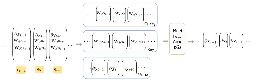
TinT Self-attention backpropagation module
The input embeddings contain in the first coordinates. Since we require to re-compute the attention scores , we need to copy the query, key, and value vectors , , and from the TinT self-attention Forward module at each position . Furthermore, we use the residual connection to copy the prefix embeddings , which contain the rows of , from the TinT self-attention Forward module.
The operation can be divided into three sub-operations: Computing (a) attention scores for all , at each position , (b) from and , and (c) from .
-
•
Sub-operation (a): Since, the current embeddings contain , we can simply call a self-attention attention module to compute the attention scores for all and store them in the current embeddings. We further retain and for further operations using residual connections.
-
•
Sub-operation (b): With the current embeddings containing the attention scores for all , and the gradient , we can compute using a TinT linear self-attention module with atleast attention heads, that represent the attention scores between tokens and for any as and use as their value vectors.
-
•
Sub-operation (c): And finally, the computation of is identical to the backpropagation through a linear layer, with parameters and . Hence, we call a Linear backpropagation module on the current embeddings, that contain and the prefix embeddings that contain and .
Separating sub-operations (a) and (b)
The operation for computing in Definition E.3 looks very similar to the computation of in Equation 9. However, the major difference is that instead of the attention scores being between token and any token , we need the attention scores to be . Thus, unless our model allows a transpose operation on the attention scores, we need to first store them in our embeddings and then use an additional self-attention module that can pick the right attention scores between tokens using position embeddings. Please see Figure 8.
Auxiliary’s value descent update
Similar to the complexity of true backpropagation, the descent updates for are quite expensive to express with the transformer layers. Hence, we focus simply on updating on , while keeping the others fixed.
Definition E.6 (Auxiliary self-attention value descent).
For query, key, and value weights and bias , the value descent layer corresponding to a self-attention layer with attention heads and any function takes in a batch of gradients and inputs and updates as follows:
Here, refers to value vectors at each position , as defined in Definition E.1.
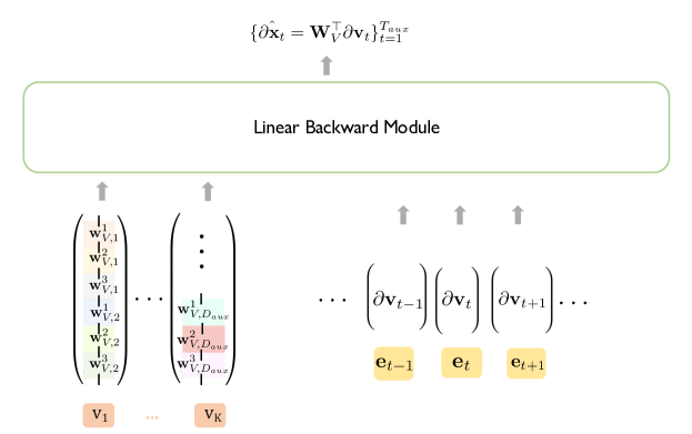
TinT Self-attention descent module
The input embeddings contain in the first coordinates, from the TinT self-attention backpropagation module. Furthermore, the prefix embeddings contain the stacked rows of and , continuing from the TinT self-attention backpropagation module.
Since we further need the input to the auxiliary self-attention layer under consideration, we use residual connections to copy from the TinT self-attention Forward module at each position .
The updates of and are equivalent to the parameter update in a linear layer, involving gradients and input . Thus, we call a Linear descent module on the current embeddings and the prefix embeddings to get the updated value parameters. Please see Figure 9.
E.1 Proofs of theorems and gradient definitions
We restate the theorems and definitions, before presenting their proofs for easy referencing.
See E.2
Derivation of gradient in Definition E.2.
Recalling the definition of from Definition E.1,
denote , , and respectively for all , and . is defined with its rows as for all .
We explain the proof for an arbitrary token position . With the application of the chain rule, we have
where the second step follows from the definitions of and respectively.
Computation of :
With the Split operation of across heads for the computation of , the computation of the backpropagated gradient itself needs to be split across heads. Furthermore, query vector only affects , implying for any . Thus, we have for any head , if represents the output of attention head , given by ,
| (11) | ||||
| (12) | ||||
| (13) | ||||
In Equation 11, we have expanded the definition of in in order to better motivate the derivative of w.r.t. . Finally, is given by
Computation of :
Continuing as the computation of , we split the computation of across the attention heads. However, unlike , affects for all . For any head , we follow the chain-rule step by step to get
| (14) | ||||
| (15) | ||||
| (16) | ||||
| (17) | ||||
| (18) | ||||
In Equation 14, we separate the inside sum into two components, since the derivative w.r.t. differ for the two components, as outlined in the derivation of Equation 17 from Equation 15, and Equation 18 from Equation 16. We have skipped a step going from Equations 16 and 15 to Equations 17 and 18 due to typographical simplicity. The skipped step is extremely similar to Equation 12 in the derivation of Finally, is given by
Computation of :
Similar to the gradient computation of , the computation of needs to be split across the attention heads. However, like , affects for all . For any head , we follow the chain-rule step by step to get
∎
See E.5
Proof of Theorem E.5.
For typographical simplicity, we discuss the proof at an arbitrary position . Recall the definition of an -hard attention head from Definition E.4. An attention head is defined to be -hard on an input sequence , if for each position , there exists a position such that the attention score .
For the proof, we simply focus on , and the proof for follows like-wise.
Bounds on :
Recalling the definition of from Definition E.2, we have
Focusing on a head , define and as the token position where the attends the most to, i.e. and . Then,
where the final step uses a Cauchy-Schwartz inequality. We focus on the two terms separately.
-
1.
: Focusing on , we have
(19) We use a Cauchy-Schwartz inequality in the second and third steps and the attention head behavior in the final step.
Hence, can now be bounded as follows:
In the final step, in addition to the bound from Equation 19, we use a Cauchy-Schwartz inequality to bound and bound the attention score by .
-
2.
: Focusing on for any , we have using two Cauchy-Schwartz inequalities:
(20) Hence,
In the final step, in addition to the bound from Equation 20, we use a Cauchy-Schwartz inequality to bound and use the -hard behavior of the attention head to bound
Combining the bounds on both terms, we have
We bound the remaining terms as follows.
-
•
, under the bounded assumption of the gradients.
-
•
For any , we have since . Furthermore, from the defintion of the key vector , with a Cauchy-Schwartz inequality. Under the bounded assumptions of and input , we have
-
•
Similar procedure can be followed for bounding .
Thus, we have
Bounds on :
From the definitons of and from Definitions E.3 and E.3, we have
where we use Cauchy-schwartz inequality in the second step. We use the assumed bounds on , and the computed bounds on in the pre-final step. ∎
Appendix F Layer normalization
Definition F.1.
[Layer Normalization] Define a normalization function that performs , where and are the mean and standard deviation of , respectively. Then, layer normalization with parameters takes as input and outputs , which is computed as
Definition F.2.
[Exact Gradient for Layer Normalization] Using notations in Definition F.1, given the gradient of the loss w.r.t the output of the Layer Normalization , backpropagation computes as
Exact backpropagation is expensive because requires using at least two sequential MLPs. We thus approximate it with a first-order Taylor expansion, which is entry-wise close to the true gradient.
Definition F.3.
[-approximate Layer Normalization Gradient] With notations defined above, this layer takes as input and outputs
In the discussions below, we consider a layer normalization layer in the auxiliary model with parameters that takes in input sequence and outputs , with for each . Since this involves a token-wise operation, we will present our constructed modules with a general token position and the prefix tokens We will use as a diagonal matrix in , containing on its main diagonal.
TinT Layer normalization Forward module
The input embedding to this module will contain in its first coordinates. The layer normalization computation can be divided into two sub-operations: (a) application of , and (b) linear computation using . We will present a TinT module for each sub-operation.
We can represent the function using a layer normalization operation itself, with its weight and bias parameters set as and respectively. However, since the relevant input exists only in the first coordinates, the operation on the first coordinates needs to be independent of the rest of the coordinates. To do so, we instead use Group normalization (Definition F.6) on , with groups of size .
Now, the embedding contains in its first coordinates. The second sub-operation can then be viewed as a Linear Layer computation, i.e. . Hence, we simply stack the rows of and onto the prefix tokens and call the TinT Linear Forward module (Appendix D).
Auxiliary’s gradient backpropagation through layer normalization
With the definition of layer normalization and the normalization function in Definition F.1, the auxiliary’s backpropagation operation takes in the loss gradient w.r.t. output () and computes the loss gradient w.r.t. input ().
See F.2
Complexity of true backpropagation
The above operation is computation heavy since it involves computing (a) , (b) , (c) , and (d) multiplying by a factor of . in itself will require two MLP layers, following Lemma C.4. In order to reduce the number of layers, we turn to first-order Taylor expansion for approximating the above operation.
See F.3
The following theorem shows that the first-order gradient is a good approximation of the true gradient, and in the limit of tending to , the approximation error tends to as well.
Theorem F.4.
For any , and a layer normalization layer with parameters , for an input and gradient ,
where denotes the standard deviation of . have been computed from , and using Definitions F.2 and F.3.
TinT Layer normalization backpropagation module
The input embeddings contain at each position in the first coordinates. Since we further need the input to the auxiliary’s layer normalization layer under consideration, we copy from the TinT Layer normalization Forward module at each position using residual connections. Furthermore, residual connections have been used to copy the contents of the prefix tokens from the Layer normalization Forward module, which contain . Recall that for ease of presentation, we use to represent .
We set as a hyperparameter and return as the output of this module. The computation of can be divided into two sub-operations: (a) computation of , and (b) computation of . We represent each sub-operation as a TinT module.
To compute , we can observe that the required operation is identical to backpropagating through a linear layer with parameters and . Hence, we simply call the Linear Backpropagation module on the current embeddings. We use residual connections to retain at each location , and the contents of the prefix tokens .
Now, the embedding contains and . In order to backpropagate through , we first use a linear layer to compute and retain . Following the same procedure as the Forward module, we use a Group normalization layer with weight and bias parameters and respectively, to compute and . Finally, we use a linear layer to compute
Auxiliary’s Descent update
And finally, the auxiliary’s descent operation updates parameters using a batch of inputs and the loss gradient w.r.t. the corresponding outputs .
Definition F.5 (Auxiliary’s layer normalization descent).
For parameters , descent update takes in a batch of inputs and gradients and updates the parameters as follows:
where represents .
The update of involves an elementwise multiplication between and , which requires an MLP layer (Lemma C.4). With the prefix tokens containing the rows of and , we instead consider the update of alone with the descent update.
TinT Layer normalization descent module
The input embeddings contain in the first coordinates. The prefix tokens contain , which have been copied from the Forward module using residual connections. The update of is identical to the auxiliary’s descent update through a linear layer. Hence, we apply a TinT Linear descent module to the current embeddings, updating only the bias and switching off the update to
F.1 Additional definitions
We describe TinT group normalization layer below, which we use in different modules to simulate the auxiliary’s layer normalization operations.
Definition F.6 (TinT -Group normalization).
Define a normalization function that performs , where and are the mean and standard deviation of , respectively. Then, -Group RMSnorm with parameters takes as input and outputs , with
where
F.2 Proof of theorems and gradient definitions
We restate the theorems and definitions, before presenting their proofs for easy referencing.
See F.2
Derivation of gradient in Definition F.2 .
With the normalization function and parameters , recall from Definition F.1 that given an input , a layer normalization layer returns Let and denote the mean and standard deviation of . They can be computed as
With the chain rule, we can compute from as follows.
| (21) |
Since , we have , where represents a diagonal matrix with on the main diagonal. Thus,
With , we have
| (22) |
In the final step, we require and , which are computed as follows.
-
•
with its th element given by
-
•
with its th element given by
where we have re-utilized the in the pre-final step.
Hence, from Equation 21,
∎
We repeat Theorem F.4 for easier reference. See F.4
Proof of Theorem F.4 .
With the normalization function and parameters , recall from Definition F.1 that given an input , a layer normalization layer returns Let and denote the mean and standard deviation of . They can be computed as
We will refer to from Equation 22 and the formulation of from Equation 21 for our current proof. To recall, they are
Using a second-order Taylor expansion of the normalization function around , we have
where represents . The second step follows similar steps for computing in Equation 22. We avoid this computation since we only need to make sure that the second-order term is bounded. Furthermore, if we can show the -norm of the second-order term can be bounded by We avoid this computation as well.
Thus, from the above formulation, we have
The pre-final step follows from Equation 22, where can be shown to be symmetric. The final step follows from the gradient formulation in Equation 21. Including the error term, we have the final bound as
Using and a Cauchy-Schwartz inequality gives the final bound. ∎
Appendix G Activation layer
Definition G.1 (Auxiliary activation).
For a continuous function , an activation layer takes as input and outputs with for all .
In the discussions below, we consider an activation layer in the auxiliary model with activation function that takes in input sequence and outputs , with for each . Since this involves a token-wise operation, we will present our constructed modules with a general token position . Since no parameters of the auxiliary model are involved in this operation, the prefix tokens contain in the following modules.
TinT Activation Forward module
The embedding contains in its first indices. We simply pass the embeddings into activation , which returns in its first indices.
Auxiliary’s backpropagation through activation
With the definition in Definition G.1, the auxiliary’s backpropagation takes in the loss gradient w.r.t. output () and computes the loss gradient w.r.t. input (). We further assume that the derivative of is well-defined everywhere. This assumption includes non-differentiable activation functions with well-defined derivatives like .
Definition G.2 (Auxiliary activation backpropagation).
For a continuous function , with a well-defined derivative for each , the backpropagation takes as input and outputs
where with at each
Complexity of true backpropagation
The above operation is computation heavy since it involves . As mentioned for the layer normalization module, the element-wise multiplication between and will require an MLP module following Lemma C.4. Furthermore, it involves changing the activation function in TinT in specific modules to . To circumvent this, we instead turn to a first-order Taylor approximation.
Definition G.3 (Approximate Activation backpropagation).
For a continuous function and a hyperparameter , the layer takes as input and outputs
The following theorems show that under mild assumptions on the activation function and the input, gradient pair, the first-order gradient is a good approximation to the true gradient.
Theorem G.4.
For any , , consider a second-order differentiable activation function , with bounded by for each . Then, for any input and gradient with , the following holds true:
where have been defined using , and in Definitions G.2 and G.3.
For activation, which is not second-order differentiable at , we instead bound the difference between by defining some form of alignment between input and gradient pair .
Definition G.5 (-alignment).
Input and gradient are said to be -aligned, if there exist a set , with , such that for each in ,
controls the fraction of coordinates where . As , as well for bounded gradients.
Example G.6.
For any , all inputs that satisfy , and gradients that satisfy , are -aligned.
Theorem G.7.
For any and , for any input and gradient , with , that are -aligned by Definition G.5,
where have been defined using , and in Definitions G.2 and G.3.
TinT Activation backpropagation module
The input embeddings contain in the first embeddings. With the requirement of the activation layer input for gradient, we copy from the Forward module at each position . We set as a hyper-parameter and return as the output of this module.
will be computed using a single-layer MLP with activation as follows. The first linear layer of the MLP will be used to compute and . After the activation , the embedding contains and . The final linear layer of the MLP will be used to compute .
G.1 Proofs of theorems
We restate the theorems, before presenting their proofs for easy referencing.
See G.4
Proof.
The proof follows along the lines of Theorem F.4. Recall that given an input , the activation layer outputs , where the function is applied coordinate-wise on . Given input and the output gradient , the gradient w.r.t. the input is given by , where the function is also applied coordinate wise to . We defined as an -approximate gradient, given by Since both and are applied coordinate-wise, we can look at the coordinate-wise difference between and .
Consider an arbitrary coordinate . Under the assumption that is second-order differentiable, we have
where represents in the second step. In the final step, we utilize the upper bound assumption on
Thus, , and so
∎
See G.6
Proof.
Recall the definition of -alignment from Definition G.5. Input and gradient are said to be -aligned, if there exist a set , with , such that for each in ,
Consider an arbitrary coordinate . We have for any . Under the assumption that , and , a bound of suffices. ∎
See G.7
Proof.
Recall that given an input , the activation layer outputs , where the function is applied coordinate-wise on . Given input and the output gradient , the gradient w.r.t. the input is given by , where the function is also applied coordinate wise to . We defined as an -approximate gradient, given by Since both and are applied coordinate-wise, we can look at the coordinate-wise difference between and . For activation, for all , with to avoid ambiguity.
Going by the definition of -alignment of the input and gradient from Definition G.5, we have a set with such that for each , . For all coordinates , we can then observe that , implying
For coordinates , we have three possible cases:
-
•
: In this case, we can again show
-
•
, : In this case, we have , and so . Additionally, , and so
where in the final step, we use the fact that and
-
•
, : In this case, we have , and so . Additionally, , and so
where in the final step, we use the fact that and
Thus, from the above discussion, we have
The final step includes a simple Cauchy Schwartz inequality and the desired bound comes from the assumed bound on . ∎
Appendix H Language model head
Additionally, we provide a description of the gradient computation for the loss function that involves the language model head. This computation entails performing a operation over the entire vocabulary. If denotes the vocabulary set of the auxiliary model, and denotes the embedding matrix of the auxiliary model, we directly utilize the embedding matrix for the auto-regressive loss in the TinT. Additionally, we do not update the embedding matrix of the auxiliary model; instead, we solely backpropagate the gradients through the language model head. Recent work in (Kumar et al., 2022) has shown that keeping the embedding matrix fixed while updating the model can stabilize SGD. We demonstrate that the backpropagated gradients can be expressed as the combination of the language model head and a self-attention layer.
Definition H.1 (KL-loss gradient through auxiliary’s language model head).
Given an embedding matrix , the language model head takes in input and a target distribution and returns gradient , with
In the autoregressive loss on a sequence of tokens, the target output distribution at any position is the next occurring token. If denote the uncontextualized embeddings of a sequence of tokens after encoding them via the embedding matrix, and denote their contextualized embeddings after passing through the auxiliary model, then the gradient at any position can be simplified as We illustrate the involved TinT module w.r.t. an arbitrary position .
TinT autoregressive loss gradient module
The current embedding contains the contextualized embedding in its first coordinates. Furthermore, includes the uncontextualized embedding , copied from the input layer using residual connections. The prefix tokens are assigned a value of and do not participate in the subsequent computations.
The loss computation can be decomposed into two sub-operations: (a) computing , and (b) calculating .
For the first sub-operation, we use a feed-forward layer with activation, with hidden and output weights and respectively, that takes in the first of and returns in the first coordinates. We retain using a residual connection.
The final sub-operation can be interpreted as a TinT self-attention layer. With containing both and , we use a linear self-attention layer (Definition C.1) with two attention heads. The first attention head assigns an attention score of to pairs , while assigning an attention score of to the remaining pairs. At any position , is considered the value vector. The second attention head assigns an attention score of to pairs , while assigning an attention score of to the remaining pairs. At any position , is considered the value vector. The outputs of both attention heads are subsequently combined using a linear layer.
Remark H.2.
We conducted experiments using mean-squared loss and Quad loss (Saunshi et al., 2020), which do not necessitate softmax computations for gradient computation. As an example, in the case of mean-squared loss, if our objective is to minimize , the gradient can be computed as . Similarly, in the case of Quad loss, the gradient is . However, in all of our language model experiments (Section 5), both gradients resulted in minimal improvement in perplexity compared to the auxiliary model. Therefore, we continue utilizing the standard KL loss for optimization.
Remark H.3.
For ease of implementation in the codebase, we utilize a dedicated loss module that takes in as input and directly computes .
Appendix I Parameter sharing
Feed-forward layer of auxiliary model:
In a standard auxiliary transformer, like GPT-2, the feed-forward layer is a token-wise operation that takes in an input and returns , with and . A naive construction of the TinTto simulate its forward operation will have 2 Linear Forward modules (Section 3), separated by an activation. However, this requires more prefix embeddings to represent the parameters, compared to other linear operations in the auxiliary transformer that use weight parameters.
To avoid this, we can instead break down the computation into 4 sub-feed-forward layers, each with its own parameters . Here represent -shards of the rows of , and represent -shards of the columns of . The forward, backward, and descent operations on these 4 sub-feed-forward layers can be effectively parallelized. For example, the forward operation of each layer can be simulated by a single TinTmodule, consisting of two Linear Forward modules and activation, changing only the prefix embeddings to correspond to .
Appendix J Additional modules
We describe the forward, backward, and decent update operations of additional modules, used in different model families, like LLaMA (Touvron et al., 2023) and BLOOM (Scao et al., 2022). We discuss the simulation of these modules, using similar TinT modules.
J.1 Root mean square normalization (RMSnorm)
The operation of RMSnorm (Zhang & Sennrich, 2019) is very similar to layer normalization.
Definition J.1 (RMSnorm).
For an arbitrary dimension , define a normalization function that performs , where Then, RMSnorm with parameters takes as input and outputs , which is computed as
The extreme similarity between RMSnorm and layer normalization (Definition F.1) helps us create similar TinT modules as described in Appendix F, where instead of Group normalization layers, we use Group RMSnorm layers described below.
Definition J.2 (TinT -Group RMSnorm).
For an arbitrary dimension , define a normalization function that performs , where Then, -Group RMSnorm with parameters takes as input and outputs , with
where
J.2 Attention variants
In order to incorporate additional attention variants, e.g. Attention with Linear Biases (ALiBi) (Press et al., 2021), and rotary position embeddings (Su et al., 2021), we can change the definition of softmax attention layer in Definition C.1 likewise.
We showcase the changes for ALiBi.
Definition J.3 (Auxiliary ALiBi self-attention with heads).
For query, key, and value weights , bias and , ALiBi self-attention layer with attention heads and a function takes a sequence as input and outputs , with
| (23) |
is defined as the attention score of head between tokens at positions and , and is given by
| (24) |
Here denotes a relative position vector at each position that contains at each coordinate . Here, , , denote the query, key, and value vectors at each position , computed as , , and respectively. In addition, denote , , and respectively for all , and . is defined with its rows as for all .
To include operations involving ALiBi, we modify the self-attention module of TinT to change the definition of the attention scores like Equation 24.
Definition J.4 (Modified TinT self-attention for ALiBi with heads).
For parameters , , , and , TinT self-attention with attention heads and a function takes a sequence as input and outputs , with
Here denotes a relative position vector at each position that contains at each coordinate . Here, , , denote the query, key, and value vectors at each position , computed as , , and respectively. is defined with its rows as for all .
After referring to Appendix E, we make the following modifications to the Forward, Backward, and Descent modules. In the Forward module, we incorporate the modified self-attention module to compute the attention scores using ALiBi attention. In the Backward module, since we do not propagate gradients through the attention scores of the auxiliary model, the backpropagation formulation remains unchanged from Definition E.3 when we have access to the attention scores. Similarly, in the Descent module, we update the value matrix while keeping the query and key parameters fixed. The formulation of the gradient update remains unchanged from Definition E.6 when we have access to the attention scores. Consequently, we simply modify all the self-attention modules in the simulator to include ALiBi attention, as defined by Definition J.4.
J.3 Gated linear units (GLUs)
We describe the operations of GLUs (Shazeer, 2020) using similar GLU units available to the TinT.
Definition J.5.
For parameters , and biases , a GLU layer with activation , takes input and outputs , with
Typical GLUs have as a hidden dimension (i.e. the dimension of ). We can use similar parameter-sharing techniques discussed for feed-forward layers (Appendix I) with the TinT modules presented here. Furthermore, since can be expressed as a combination of the gated operation and a linear operation, we focus on the computation of here.
For the discussion below, we consider a GLU (without the output linear layer) in the auxiliary model, with parameters , that takes in input sequence and outputs , with for each . Since this involves a token-wise operation, we will present our constructed modules with a general token position and the prefix tokens
TinT GLU Forward module
The embedding contains in its first coordinates. The output can be computed using three sub-operations: (a) linear operation for , (b) linear operation for , and (c) gate operation to get .
We use three TinT modules, representing each sub-operation.
-
(a)
is a linear operation, hence we can use a TinT Linear Forward module (Appendix D) with the current embedding and containing to get embedding containing in its first coordinates.
-
(b)
is a linear operation, hence we can similarly use a TinT Linear Forward module (Appendix D) with the embedding and containing to get embedding containing in its first coordinates.
and are now combined to get an embedding that contains in its first coordinates.
-
(c)
Finally, we can use a TinT GLU layer that can carry out the elementwise multiplication of to get in the first coordinates.
Parameter Sharing: Since (a) and (b) involve a Linear Forward module, we can additionally leverage parameter sharing to apply a single Linear Forward module for each of the two computations, changing only the prefix embeddings to correspond to , or .
Auxiliary GLU backpropagation
For the GLU layer defined in Definition J.5, the backpropagation layer takes in the loss gradient w.r.t. output () and computes the loss gradient w.r.t. input ().
Definition J.6 (Auxiliary GLU backpropagation).
For the weights , the backpropagation layer takes as input and outputs , with , where
A direct computation of involves changing the activation function to . Following a similar strategy for backpropagation through an activation layer (Appendix G), we instead use a first-order Taylor expansion to approximate .
Definition J.7 (Auxiliary GLU approximate backpropagation).
For a hyper-parameter , for the weights , the approximate backpropagation layer takes as input and outputs , with , where
TinT GLU backpropagation module
The current embedding contains in its first coordinates. Furthermore, since we need and in the gradient computations, we copy them from the Forward module using residual connections. We discuss the computation of and as separate sub-modules acting on the same embedding in parallel.
-
1.
The computation of involves two sub-operations: (a) gate operation to get , and (b) linear backward operation to get . Since for this operation, we require , we copy the contents of the prefix embeddings containing from the Forward module.
-
(a)
Since the current embedding contains both and , we can use a TinT GLU layer to get an embedding that contains .
-
(b)
The final linear backward operation can be performed by using a TinT Linear backpropagation module (Appendix D) with the embeddings and the prefix embeddings. The final embedding contains in the first coordinates.
-
(a)
-
2.
The computation of involves four sub-operations: (a) gate operation to get , (b) gate operation to get , (c) a linear layer to compute , (c) linear backward operation to get . Since for this operation, we require , we copy the contents of the prefix embeddings containing from the Forward module.
-
(a)
Since the current embedding contains , and , we can use two TinT GLU layers to get an embedding that contains both and .
-
(b)
A linear later on can then return an embedding containing in the first coordinates.
-
(c)
The final operation can be performed by using a TinT Linear backpropagation module (Appendix D) with the embeddings and the prefix embeddings containing . The final embedding contains in the first coordinates.
-
(a)
After the two parallel computations, we can sum up and to get an embedding containing (Definition J.7) in the first coordinates.
Auxiliary GLU descent
Finally, the auxiliary’s descent updates the weight and the bias parameters using a batch of inputs and the loss gradient w.r.t. the corresponding outputs .
Definition J.8 (Auxiliary GLU descent ).
For weights and bias , the linear descent layer takes in a batch of inputs and gradients and updates the parameters as follows:
where and have been computed as Definition J.6.
Due to similar concerns as gradient backpropagation, we instead use (Definition J.7) in place of for each to update
TinT GLU descent module
We discuss the two descent operations separately.
-
1.
Update of : We start with the embeddings from the backpropagation module, that contain in the first coordinates.
For the update, we additionally require the input to the auxiliary GLU layer under consideration, and hence we copy from the Forward module using residual connections. Furthermore, we copy the contents of the prefix embeddings that contain from the Forward module.
With both and in the embeddings, the necessary operation turns out to be the descent update of a linear layer with parameters . That implies, we can call a TinT Linear descent module (Appendix D) on the current embeddings and prefix embeddings to get the desired update.
-
2.
We start with the embeddings from the backpropagation module, that contain in the first coordinates.
For the update, we additionally require the input to the auxiliary GLU layer under consideration, and hence we copy from the forward module using residual connections. Furthermore, we copy the contents of the prefix embeddings that contain from the Forward module.
With both and in the embeddings, the necessary operation turns out to be the descent update of a linear layer with parameters . That implies we can call a TinT Linear descent module on the current embeddings and prefix embeddings to get the desired update.
Parameter sharing: Since both the descent updates involve a Linear descent module, we can additionally leverage parameter sharing to apply a single TinT Linear descent module for each of the two computations, changing the input to correspond to and prefix to correspond to , or the input to correspond to and prefix to correspond to respectively.
Appendix K Construction of other variants of pre-trained models
Though we only conduct experiments on an OPT-125m model, our construction is generally applicable to diverse variants of pre-trained language models. Table 3 highlights many types of modules and the required size and computation for each. The size of a constructed model is influenced by various factors, including the number of layers, and embedding dimension in the auxiliary.
Appendix L Experiments
| Model | Shots | Subj | AGNews | SST2 | CR | MR | MPQA | Amazon | Avg. |
| Without Calibration | |||||||||
| OPT-125m | |||||||||
| OPT-1.3b | |||||||||
| OPT-125m Fine-tuning | |||||||||
| OPT-125m TinT | |||||||||
| OPT-125m | |||||||||
| OPT-1.3b | |||||||||
| OPT-125m Fine-tuning | |||||||||
| OPT-125m TinT | |||||||||
| With Calibration | |||||||||
| OPT-125m | |||||||||
| OPT-1.3b | |||||||||
| OPT-125m Fine-tuning | |||||||||
| OPT-125m TinT | |||||||||
| OPT-125m | |||||||||
| OPT-1.3b | |||||||||
| OPT-125m Fine-tuning | |||||||||
| OPT-125m TinT | |||||||||
Computing environment: All the experiments are conducted on a single A100 80G GPU.
Hyperparameters: In the few-shot setting, we employ three different random seeds to select distinct sets of training examples. Grid search is performed for each seed to determine the optimal learning rate for both constructed models and dynamic evaluation. The learning rates considered for the learning rate hyperparameter in the descent update operations in TinT are . 999When utilizing the full-context loss, the learning rates considered are , and due to gradient summations in TinT. Additionally, we explore various layer-step combinations to allocate a fixed budget for one full forward pass. Specifically, we update the top 3 layers for 4 steps, the top 6 layers for 3 steps, or 12 layers for 1 step.
Calibration:
Recall from Section 5 that given a downstream task input (e.g., a movie review), the model’s predicted label is computed as follows. First, we design a simple task-specific prompt (e.g., “Sentiment:”) and select label words to serve as surrogates for each class (e.g., “positive” and “negative”). Then, we provide the input along with the prompt to the model, and the label word assigned the highest probability is treated as the model’s prediction. We compare TinT to its baselines in two settings: no calibration (reported in Table 2 in the main paper), and with calibration. If using calibration, then the probabilities are normalized using just the prompt as input.101010Calibration is not applied to the language modeling evaluation.
This is a widely used calibration technique (Holtzman et al., 2021) for prompting language models.
Additional observations from Table 4, compared to Table 2:
In Table 4, we have reported the comparisons with calibration in addition to the non calibration results reported in Table 2. We observe that calibration may not always be beneficial in every setting.111111Such inconsistencies in the calibration method have been observed in previous works (Brown et al., 2020). However, even with calibration, TinT remains competitive to fine-tuning of OPT models. The performance of OPT-1.3B improves with calibration. In this case, TinT lags behind OPT-1.3B in the few-shot setting.
Results of different settings.
Table 5 displays the results of few-shot learning with calibration across various settings, encompassing different loss types, input formats, and layer-step configurations. Our analysis reveals that employing a label-only loss, utilizing a single-example input format, and updating all layers of the internal model for a single step yield the most favorable average result. The performance of the multi-example format is disadvantaged when dealing with tasks of long sequences such as Amazon Polarity. In general, we observe that calibrated results tend to be more consistent and stable.
| Loss Type | Format | Layer | Step | Subj | AGNews | SST2 | CR | MR | MPQA | Amazon | Avg. |
| Label | Single | 12 | 1 | ||||||||
| Single | 6 | 2 | |||||||||
| Single | 3 | 4 | |||||||||
| Multi. | 12 | 1 | |||||||||
| Multi. | 6 | 2 | |||||||||
| Multi. | 3 | 4 | |||||||||
| Full-context | Single | 12 | 1 | ||||||||
| Single | 6 | 2 | |||||||||
| Single | 3 | 4 | |||||||||
| Multi. | 12 | 1 | |||||||||
| Multi. | 6 | 2 | |||||||||
| Multi. | 3 | 4 |