Dark energy, D-branes, and Pulsar Timing Arrays

Abstract

Several pulsar timing array (PTA) collaborations recently announced the first detection of a stochastic gravitational wave (GW) background, leaving open the question of its source. We explore the possibility that it originates from cosmic inflation, a guaranteed source of primordial GW. The inflationary GW background amplitude is enhanced at PTA scales by a non-standard early cosmological evolution, driven by Dirac-Born-Infeld (DBI) scalar dynamics motivated by string theory. The resulting GW energy density has a broken power-law frequency profile, entering the PTA band with a peak amplitude consistent with the recent GW detection. After this initial DBI kination epoch, the dynamics starts a new phase mainly controlled by the scalar potential. It provides a realization of an early dark energy scenario aimed at relaxing the $H_{0}$ tension, and a late dark energy model which explains the current cosmological acceleration with no need of a cosmological constant. Hence our mechanism – besides providing a possible explanation for the recent PTA results – connects them with testable properties of the physics of the dark universe.

1 Introduction

Cosmic inflation, well tested at large CMB scales, is a guaranteed source of primordial tensor fluctuations [1, 2, 3, 4, 5]. However, their amplitude is typically too small to be directly detected by gravitational wave (GW) experiments. In this work we explore a post-inflationary mechanism capable of enhancing the size of inflationary tensor fluctuations at frequencies detectable by pulsar timing arrays (PTA) (for other examples of post-inflationary mechanisms, see [6, 7, 8]). The GW energy density parameter $\Omega_{\rm GW}$ depends on the early-time behavior of the cosmological scale factor, which can be influenced by the presence of stiff matter [9, 10, 11], or scalar fields coupled conformally [12, 13, 14, 15, 16, 17] or disformally [18, 19] to the metric. Extending the results of [19], we show that an early epoch of scalar domination – motivated by a quantum gravity approach to early-universe cosmology – induces a non-standard cosmological evolution, which enhances the amplitude of $\Omega_{\rm GW}$ at frequencies around $10^{-8}$ Hz. Our framework provides a possible contribution towards the explanation of the recent detection of a stochastic GW background, as announced by several PTA collaborations: NANOGrav [20], PPTA [21], EPTA [22], CPTA [23] (see also e.g. [24, 25] for some of their own preliminary interpretations in terms of early universe sources). At the same time, it may ameliorate some well-known cosmological problems related with the Hubble tension (see [26, 27] for reviews), and the nature of dark energy.

We start with a theoretical section 2 developing our string-motivated set-up based on the dynamics of a D-brane in a higher-dimensional space-time. The D-brane motion through extra-dimensional angular directions is described in terms of an axionic field, coupled to four-dimensional gravity, and to matter living on the brane through a disformal coupling [28]. The scalar-tensor action includes a kinetic term of Dirac-Born-Infeld (DBI) form, which is instrumental in controlling an initial phase of kinetically-driven scalar evolution that enhances the GW spectrum. Moreover, the Lagrangian includes a potential term, responsible for driving both an early and a late dark energy dominated epoch (for an example of a cascading dark energy scenario, see [29]).

We continue with a phenomenological section 3, which starts examining how the initial scalar dynamics drives an initial epoch of coupled DBI kination. This phase affects the early evolution of the Hubble parameter, enhancing the size of the inflationary SGWB spectrum, which acquires a broken power-law profile with a peak amplitude well within the sensitivity curves of PTA experiments. Interestingly, the characteristic scale controlling the DBI kination is comparable with the scale of QCD transition. We compare the peak amplitude of our profile with recent data from NANOGrav collaboration [20], finding overall agreement.

After examining the consequences of our set-up for GW physics, in section 3.2 we discuss how the initial DBI kination phase is connected to a stage where the scalar dynamics is mainly controlled by a string-motivated axion potential. The structure of the axion potential is determined by the isometries of the extra-dimensional space, as well as non-perturbative effects. It can be sufficiently rich to first drive a phase characterized by early dark energy – which can address the Hubble tension – followed by a late dark energy epoch, which can explain the current acceleration of our universe. Interestingly, the corresponding axion decay constants acquire sub-Planckian values. They might represent an acceptable set-up for building models of dark energy within string theory (see e.g. [30] for a review).

2 Our set-up

In this section we discuss the effective action for a string-motivated D-brane system. It can be described in terms of a scalar-tensor theory with interesting consequences for cosmology and the physics of gravitational waves. Our scenario is motivated by D-brane scalar-tensor theories as discussed in [31]: we consider a (stack of) D-brane(s) moving along the angular direction of an internal warped compactification. The axion field $\phi$ is associated with the angular position of the brane through the extra-dimensional space. The system is described by a scalar-tensor theory characterized by disformal couplings to matter fields on the brane [28] (see [32] for a review). The reader interested in more general scenarios – including conformal couplings between the scalar and the metric – can consult [17, 18, 33, 19].

The scalar-tensor action we consider is:

$$S_{\rm tot}\,=\,S_{\phi}+S_{\rm m},$$ (2.1)

where

$$S_{\phi} = \int d^{4}x\,\sqrt{-g}\,\left[\frac{R}{2\kappa^{2}}-M^{4}\,\sqrt{1+\frac{(\partial\phi)^{2}}{M^{4}}}+M^{4}-{V}(\phi)\right]\,,$$ (2.2)

$$S_{\rm m} = -\int d^{4}x\,\sqrt{-g}\,{\cal L}_{\rm m}(\tilde{g}_{\mu\nu})\,.$$ (2.3)

$\kappa^{2}=M_{{}_{\rm Pl}}^{-2}=8\,\pi\,G$, and $M$ is a mass scale entering in the scalar kinetic term, related to the (possibly warped) tension of the D-brane, as well as other properties as warping and fluxes. Matter fields contained in action (2.3) are disformally coupled to the metric $g_{\mu\nu}$ entering in eq (2.2) via

$$\tilde{g}_{\mu\nu}\,=\,g_{\mu\nu}+\frac{\partial_{\mu}\phi\,\partial_{\nu}\phi}{M^{4}}\,.$$ (2.4)

We assume that matter is a perfect fluid, characterized by pressure and energy density only (see [31] for details).

The scalar kinetic terms have the characteristic Dirac-Born-Infeld (DBI) form of D-brane actions [34]. The scalar potential $V(\phi)$ in eq (2.2) contains various contributions, which are periodic functions of the size of the internal angular dimensions. We focus on the case of a D-brane fixed at a specific value of the radial component along the (warped) extra dimensions. Its position is also fixed within four internal angular directions, leaving the object free to move along only one angular direction in the warped compact space. The motion of the brane through this angular direction is controlled by the axion field $\phi$ appearing in the scalar-tensor actions (2.2). See e.g. [35, 36] for a scenario where this idea is explicitly explored to realise natural inflation with D3 and D5 branes in a warped resolved conifold geometry [37, 38, 39].

Let us be a bit more explicit about the structure of the axion potential. The D-brane scalar potential entering eq (2.2) acquires the schematic form [40, 35]:

$$V(\theta)=\bar{V}(\rho_{0})+\delta\left(\overline{\Phi}_{-}(\rho_{0})+\Phi_{h}(\rho_{0},\theta)\right)\,,$$ (2.5)

with $\theta$ the angular direction along which the D-brane moves, that – upon canonical normalization – will give rise to the scalar field $\phi$ appearing in action (2.2). The quantity $\delta$ is a constant parameter depending on the type of D-brane considered. $\rho$ is the radial coordinate fixed at $\rho=\rho_{0}$. $\bar{V}$ and $\overline{\Phi}_{-}$ represent contributions to the D-brane potential depending only on the fixed radial coordinate $\rho_{0}$. Instead, $\Phi_{h}$ depends on the angular coordinate as well, and for a warped resolved conifold is given by [35]:

$$\Phi_{h}(\rho_{0},\theta,\phi_{0})=\sum_{l=0}^{\infty}\sum_{m=-l}^{m=l}\left[a_{l}H_{l}^{A}(\rho_{0})+b_{l}H_{l}^{B}(\rho_{0})\right]Y_{lm}(\theta,\phi_{0})\,.$$ (2.6)

The indexes $(l,m)$ denote quantum numbers associated to isometries of the internal geometry. The specific form of $H_{l}^{A},H_{l}^{B}$ is not too important, as they are functions of the fixed radial D-brane position $\rho_{0}$, only. Considering for definiteness the values $(l,m)=(0,0),(1,0),(2,0),(3,0)$, we get

$$\Phi_{h}=A_{1}(\rho_{0})+A_{2}(\rho_{0})\,\cos{\theta}+A_{3}(\rho_{0})\,\cos^{2}{\theta}+A_{4}(\rho_{0})\,\cos^{3}{\theta}\,.$$ (2.7)

For suitable choices of the coefficients, the potential for the canonically normalized field $\phi$ can be arranged to take the form

$$V_{1}(\phi)=V_{0_{\rm ede}}\left(1-\cos[\kappa\,\phi/f_{1}]\right)^{3}\,.$$ (2.8)

The quantity $f_{1}$ is an axion decay constant: we express it in terms of a dimensionless number, pulling out a factor of $\kappa$ in eq (2.8). This is the structure of the potential recently introduced for the so called early dark energy [41, 42] to relax the $H_{0}$ discrepancy. We will discuss this topic in more detail in section 3.2.

Besides the term in eq (2.8), there may be additional non-perturbative contributions to the effective potential, originating from bulk physics, which generate extra terms periodic in $\phi$. We assume that such contributions are present, and we include an additional term to the total axion potential, as [43, 44]:

$$V_{2}(\phi)=V_{0_{\rm de}}(1-\cos[\kappa\phi/f_{2}])\,.$$ (2.9)

with $f_{2}$ an extra dimensionless decay constant. To summarize, in what follows we consider the following total potential for the scalar field as a sum of two independent contributions

$$V(\phi) = V_{1}(\phi)+V_{2}(\phi)\,,$$ (2.10)

$$= V_{0_{\rm ede}}\left(1-\cos[\kappa\phi/f_{1}]\right)^{3}+V_{0_{\rm de}}\left(1-\cos[\kappa\phi/f_{2}]\right)\,.$$ (2.11)

We plug the potential (2.11) in the total action (2.2), and study the consequences of this system for the cosmological evolution of our universe.

Evolution equations

The equations of motion for the scalar field and the scale factor in a Friedmann-Lemaitre-Robertson-Walker metric, as derived from the Einstein-frame action (2.2), (2.3), are obtained to be [17, 18, 19]:

$$H^{2} =\frac{\kappa^{2}}{3}\frac{\,(1+\lambda)}{B}\rho\,,$$ (2.12a)

$$H_{{}_{N}} =-H\left[\frac{3\,B}{2(1+\lambda)}\left(1+{w}\right)+\frac{\varphi_{{}_{N}}^{2}}{2}\,\gamma\right],$$ (2.12b)

$$\varphi_{{}_{NN}} \left[1+\frac{\gamma^{-1}}{M^{4}}\,\frac{3\,B\,H^{2}}{\kappa^{2}(1+\lambda)}\right]+3\,\varphi_{{}_{N}}\left[\gamma^{-2}-\frac{{w}}{M^{4}\,\gamma}\,\frac{3\,B\,H^{2}}{\kappa^{2}(1+\lambda)}\right]$$

$$\hskip 85.35826pt+\frac{H_{{}_{N}}}{H}\,\varphi_{{}_{N}}\left[1+\frac{\gamma^{-1}}{M^{4}}\,\frac{3\,B\,H^{2}}{\kappa^{2}(1+\lambda)}\right]+\frac{3\,B\,\lambda}{\gamma^{3}\,(1+\lambda)}\,\frac{V_{,\varphi}}{V}=0,$$ (2.12c)

where the subindex $N$ indicates derivatives with respect to the number of e-folds $dN=Hdt$. For convenience we make use of the dimensionless scalar quantity $\varphi\,\equiv\,\kappa\,\phi$. We introduce the scalar-dependent Lorentz factor $\gamma$, the quantity that characterize DBI models:

$$\gamma^{-2}=1-\frac{H^{2}}{M^{4}\kappa^{2}}\,\varphi_{{}_{N}}^{2},$$ (2.13)

as well as the combinations

$$B = 1-\frac{\gamma^{2}\,\varphi_{{}_{N}}^{2}}{3\,(\gamma+1)}\,,$$ (2.14)

$$\lambda = \frac{V}{\rho}.$$ (2.15)

The parameter $\lambda$ is the characteristic quantity that controls the size of the axionic potential term with respect to the total energy density.

Since we are interested in comparing the expansion rates between our modified cosmological evolution and standard $\Lambda$CDM cosmology, we work in the Jordan frame where energy-momentum and entropy are conserved. (See the discussion in [19].) The energy density, pressure and equation of state in this frame read

$$\tilde{\rho}=\gamma^{-1}\,\rho,\qquad\tilde{p}=\gamma\,P,\qquad\tilde{w}=w\,\gamma^{2},$$ (2.16)

where the non-tilded quantities are computed in the Einstein frame. Moreover, the quantity $\tilde{\rho}=\sum_{i}\tilde{\rho}_{i}$, is the total background energy density: the index $i$ runs over matter and radiation, and $\tilde{\omega}$ takes into account of the degrees of freedom at a given temperature during cosmic evolution (see e.g. [19]). The departure from the standard cosmological evolution can thus be parameterized by the ratio of Hubble parameters in our scalar-tensor gravity, with respect to its value in General Relativity (GR) (i.e. in absence of scalar contributions):

$$\frac{\tilde{H}}{H_{GR}}=\frac{\gamma^{3/2}(1+\lambda)^{1/2}}{B^{1/2}}\,.$$ (2.17)

The evolution equations (2.12a)-(2.12c) contain contributions that modify the evolution equation with respect to $\Lambda$CDM. Any early-universe modification from the standard cosmological evolution should not occur during or after Big-Bang Nucleosynthesis (BBN), to avoid spoiling its successful predictions. Hence we require that any deviations from $\Lambda$CDM terminate before the onset of BBN: i.e., when the temperature of the universe reaches values around $T\sim$ MeV. We also investigate, however, how our system leads to late scalar-tensor contribution closely mimicking the cosmological constant of $\Lambda$CDM, driving the current acceleration of our universe. The structure of evolution equations (2.12a)-(2.12c) is such that any departure from the equation-of-state value $\tilde{w}=1/3$ does not give a noteworthy effect in the scalar evolution . In fact, in our case the most important effects in the very early evolution of the axion field $\phi$ – when the potential term contributions are negligible – are associated with the DBI form of its kinetic terms . During this phase, the amplitude of primordial gravitational waves is enhanced. As the size of the scalar potential $V(\phi)$ becomes important, additional interesting phenomenological consequences occur. These topics are the subjects of next section.

3 Phenomenology of the scalar-tensor theory

The cosmological evolution of the axionic field $\phi$ has several interesting phenomenological consequences. We assume that the initial conditions for $\phi$ are set at very high temperatures, some time after cosmic inflation. We select them such that the scalar has an initial kinetic-driven dynamics, capable of enhancing the spectrum of gravitational waves – see section 3.1. The DBI kination phase is smoothly followed by a potential-driven phase, during which the scalar dynamics source phases of early and late dark energy domination – see section 3.2.

3.1 Enhancing the gravitational wave signal at PTA scales

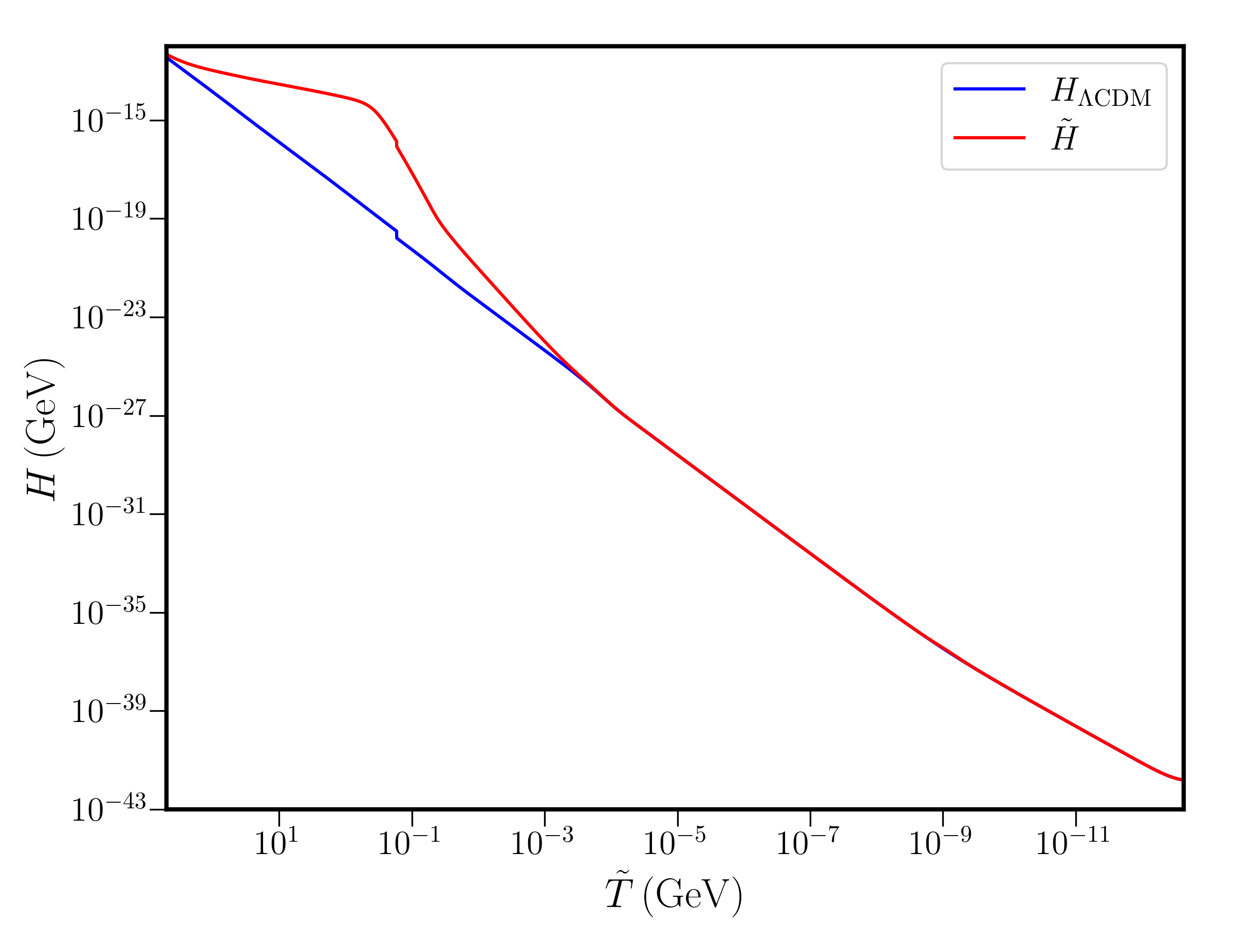
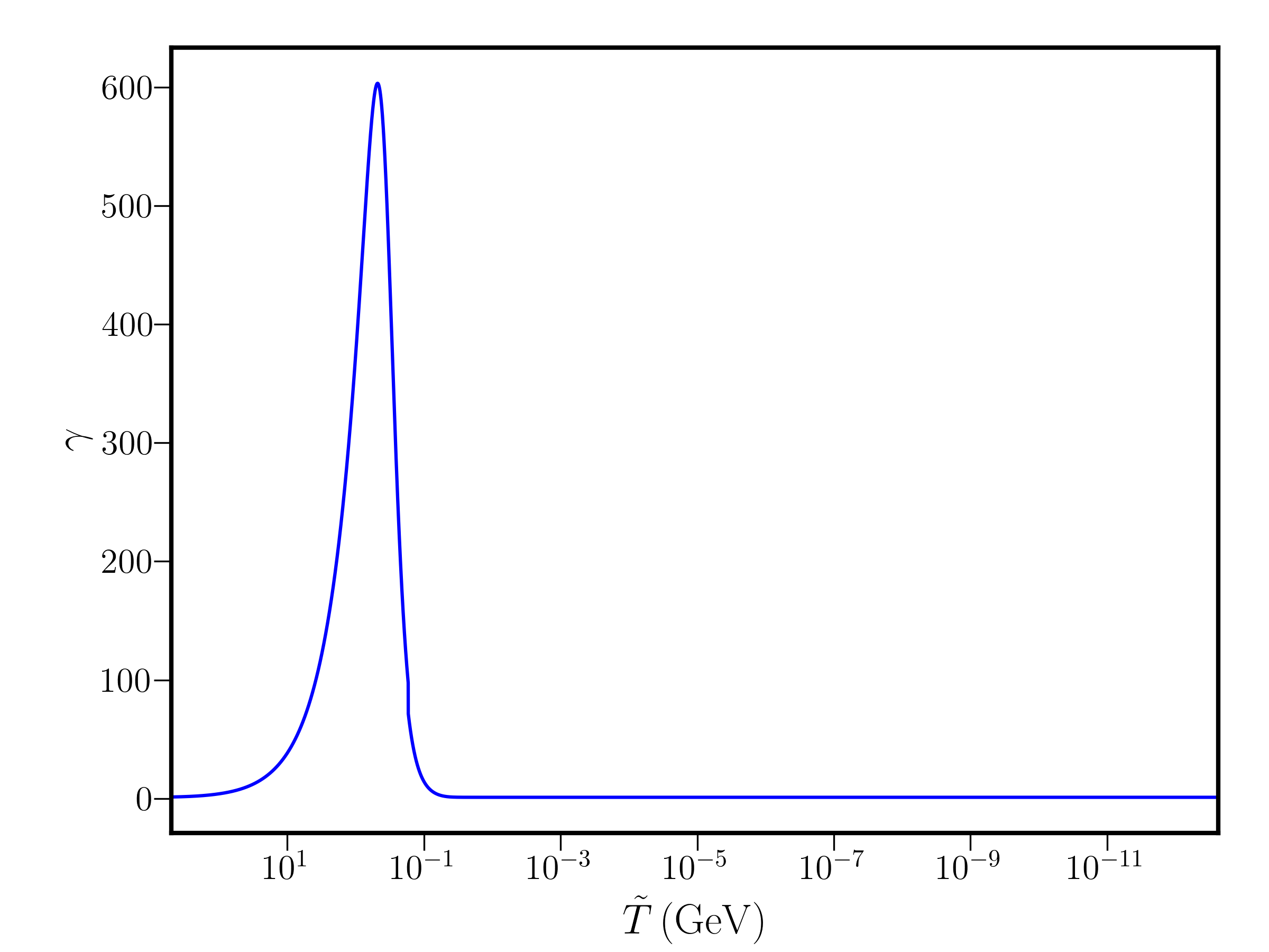
Figure 1: Left panel: Evolution of the Hubble parameter in our scalar-tensor set-up (red line) and in $\Lambda$CDM case (blue line), plotted as functions of temperature. Right panel: Evolution of the Lorentz factor $\gamma$ starting from the initial conditions in Table 1.

We show how an early modification of standard evolution associated with the DBI-type action (2.2) amplifies the amplitude of inflationary gravitational waves at PTA scales. We exploit the fact that this quantity is affected by an early-time non-standard cosmological evolution. The scalar-tensor dynamics, as controlled by the evolution equations of section 2, starts soon after inflation ends. We assume that initial conditions are chosen such that initially the scalar is driven by the DBI kinetic terms only, as appearing in action (2.2), with negligible contribution from the potential terms (see e.g. [17, 18, 19]). The parameter controlling the kinetic part of the action is $M$, whose value can chosen together with the initial conditions for $H_{i}$, $\varphi_{i}$, $\varphi_{N}^{i}$ – the last quantity entering in the initial value $\gamma_{i}$ for the DBI Lorentz parameter of eq (2.13). The initial value for $H$ is determined as described in Appendix A, starting from an initial value for the DBI parameter $\gamma_{i}$ of order ${\cal O}(1)$. Once $\varphi_{N}^{i}$ is fixed along with an initial temperature $T_{i}$ – which is associated with the initial value of the scale factor – the value of $M$ is bounded from below by requiring that the solutions for $H^{2}$ be real and positive and such as not to spoil the predictions of BBN. Assuming that entropy is conserved, the relation between the temperature of the universe $T$ and the scale factor $a$ is

$$\frac{a}{a_{0}}\,=\,\left(\frac{g_{*s,0}}{g_{*s}}\right)^{1/3}\,\frac{T_{0}}{T}\,,$$ (3.1)

where the index $0$ indicates quantities evaluated today.

$\varphi_{i}$	$\varphi_{N}^{i}$	$H_{i}$	$T_{i}$	$M$
$0.2$	$3.9\times 10^{-7}$	$3.75359\times 10^{-13}$ GeV	$499.8043$ GeV	$765$ MeV

Table 1: Initial conditions and disformal scale (recall that $\varphi$ is dimensionless and measured in Planck units).

We select initial conditions as in Table 1. The initial conditions for $\varphi$ and the Hubble parameter are chosen such as to lead to an initial steady growth of the DBI Lorentz factor $\gamma$ of eq (2.13), and a transitory large deviation of the Hubble parameter from its GR value. See Fig 1. We select the parameter $M$ demanding that the scalar evolution does not interfere with BBN, which happens around 1 MeV – see Fig 1. The value of $M$ turns out to be of the order of the QCD scale of $170$ MeV. Recall that we work in the Jordan frame – see section 2 – hence with tilded quantities.

The initial enhancement of the Lorentz factor, as well as the early modifications of the Hubble parameter, leads to an amplification of inflationary gravitational waves. The fractional energy density of primordial gravitational waves measured today is given by (we follow the treatments in [50, 51, 52, 53]):

$$\tilde{\Omega}^{0}_{\rm GW}(k) \equiv \frac{1}{\rho_{c}^{0}}\,\frac{d\,\tilde{\rho}_{\rm GW}^{0}(k)}{d\ln k}$$ (3.2)

$$\simeq \frac{1}{24}\,{\cal P}_{T}(k)\,\left(\frac{\tilde{a}_{\rm hc}}{\tilde{a}_{0}}\right)^{4}\,\left(\frac{\tilde{H}_{\rm hc}}{\tilde{H}_{0}}\right)^{2}$$ (3.3)

where ${\cal P}_{T}$ is the primordial inflationary tensor spectrum, and the suffix ‘${\rm hc}$’ indicates horizon crossing time for the mode $k$. The quantity ${\cal P}_{T}$ is

$${\cal P}_{T}(k)\,=\,\frac{2\,H^{2}}{\pi^{2}\,M_{\rm Pl}^{2}}\Big{|}_{k=aH}\,,$$ (3.4)

and we take its amplitude at CMB scales to be ${\cal P}_{T}\,=\,rA_{S}$, with $A_{S}=2.1\times 10^{-9}$. For simplicity we assume that $r$ saturates the current upper bound $r=0.036$ provided by the BICEP/Keck collaboration [54].

Formula (3.3) indicates that any deviation of the cosmological evolution from standard $\Lambda$CDM can change the predictions for $\tilde{\Omega}^{0}_{\rm GW}(k)$, and possibly amplifies the spectrum of inflationary GW. In fact, we make use of the evolution equations (2.12a)-(2.12c), and re-express $\tilde{\Omega}^{0}_{\rm GW}$ as

$$h^{2}\,\tilde{\Omega}^{0}_{\rm GW}\,=\,\left(\frac{{\cal P}_{T}}{24}\right)\,\left(\frac{\tilde{a}}{\tilde{a}_{0}}\right)^{4}\,\frac{\gamma^{3}\,H_{\rm GR}^{2}}{B\,(H_{0}/h)^{2}}\,.$$ (3.5)

The quantity $\gamma$ is given in eq (2.13), while $B$ in eq (2.14). $H_{\rm GR}$ corresponds to the GR Hubble parameter in absence of scalar field contributions. Expression (3.5) shows that an enhancement of the DBI Lorentz factor $\gamma$, and a modification of the Hubble parameter with respect its GR value influence the scale-dependence of $\Omega^{0}_{\rm GW}$. We can express this quantity as function of frequency $f=2\pi\,k\,a_{0}$, through the formula [51, 52, 55]

$$f\,=\,2.41473\times 10^{23}\,\left(\frac{T_{0}}{T_{\rm hc}}\right)\,\left(\frac{g_{*s,0}}{g_{*s,{\rm hc}}}\right)^{1/3}\,\sqrt{\frac{8\pi\rho_{\rm hc}}{3M_{\rm Pl}^{2}}}\,{\rm Hz}\,,$$ (3.6)

where recall that hc is the horizon crossing scale of the mode $k$.

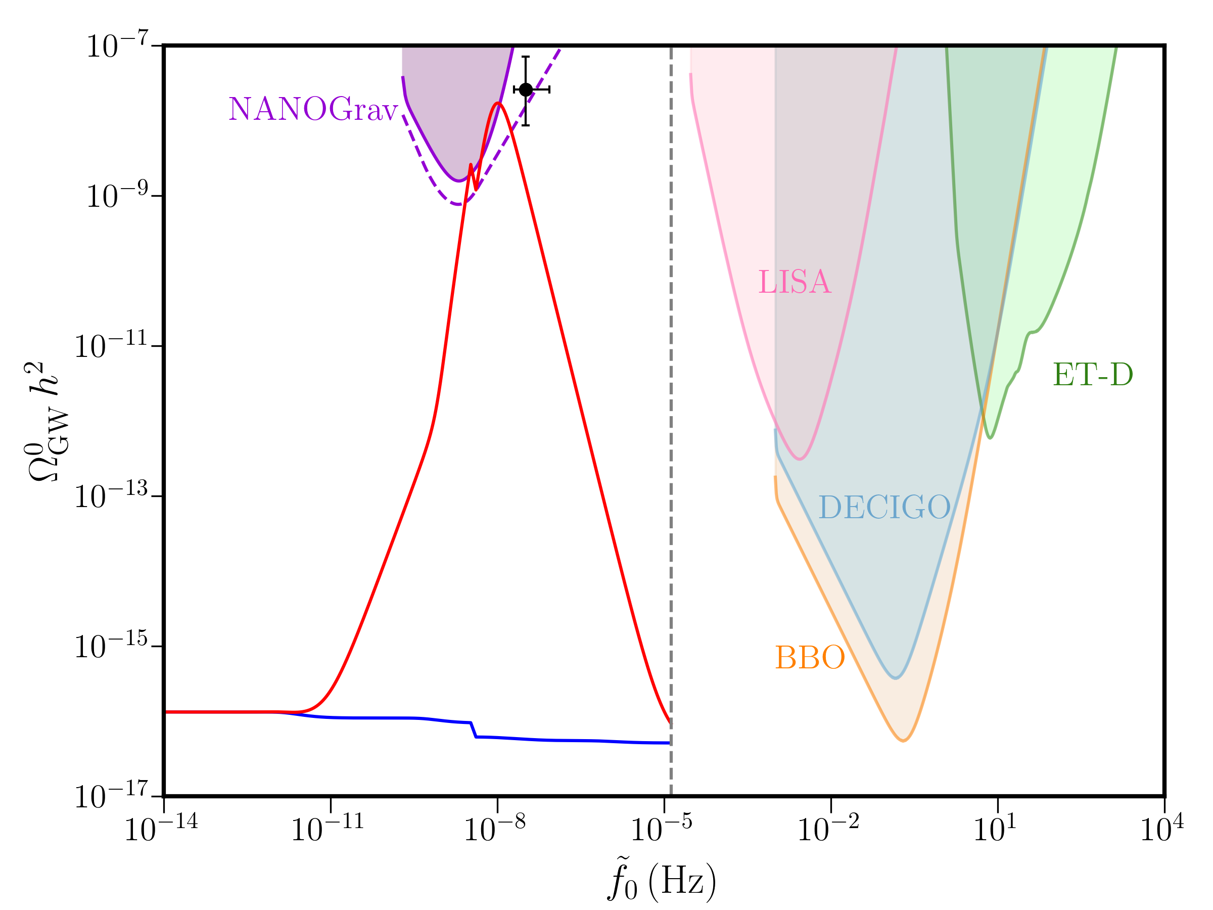
Figure 2: The profile of the primordial GW energy density of eq (3.5) in our DBI-driven scalar-tensor system (red line), as compared with the standard prediction in $\Lambda$CDM (blue line). The dashed vertical line indicates the frequency corresponding to the initial temperature $T_{i}$ at which the scalar evolution starts. The sensitivity curves for various experiments are plotted using the notion of broken power-law sensitivity (BPLS) curve [19] for ET-D, LISA, BBO, and DECIGO experiments with the condition of SNR $\geq 10$. For NANOGrav, the sensitivity curves have been constructed using the corresponding noise spectra for the stochastic gravitational wave background [56, 57]. The light violet shaded portion corresponds to the BPLS sensitivity region with SNR $\geq 5$, while the dashed violet line denotes the boundary of the power-law sensitivity (PLS) region with SNR $\geq 5$. The black point along with the y-axis error bar denotes the value $\Omega_{{}_{\rm GW}}\,h^{2}=2.6^{+4.5}_{-1.7}\times 10^{-8}$ obtained with a model of the timing-residual power spectral density with variable power-law exponent, as described by the NANOGrav collaboration [20]. This value is derived from a fiducial power-law model, which explains why it lies outside the BPLS region, but within the allowed PLS region. The x-axis error bar denotes the $90\%$ confidence region of $3.2^{+5.4}_{-1.2}\times 10^{-8}$ Hz for the break frequency in a broken power-law model as obtained by the NANOGrav collaboration [20]. The peak of the GW spectrum reaches a maximum value of $\sim 1.7\times 10^{-8}$, in agreement with the above bound, while the peak in the profile occurs at around $\sim 1.02\times 10^{-8}$ Hz.

We represent in Fig 2 the GW spectrum obtained by numerically solving the evolution equations of section 2, and plugging the results in eq (3.5). The initial conditions in Table 1 lead to a rapid, transient increase of $\gamma$, and allow us to amplify the GW signal at PTA frequencies. In fact, the energy density associated with primordial gravitational waves is raised by several orders of magnitude with respect to its standard value, for a frequency around the $10^{-9}-10^{-8}$ Hz band that is probed by PTA experiments. The frequency profile of the spectrum acquires a broken power-law shape. It initially rises as $f^{2}$, to then grow as $f^{5}$ up to the peak, and then decreases as $f^{-3}$. The peak amplitude is of the same order as the value detected by the NANOGrav collaboration [20]. However, the NANOGrav value we compare with is based on a fiducial power-law model, and a more sophisticated data analysis would be needed for comparing our broken power-law shape with the amplitude obtained by PTA data. In fact, [20] also provides a brief analysis of broken power-law models, providing the best-fit value for the break of the frequency profile: our result is consistent with their value.

Figure 2 also contains the sensitivity curves for the NANOGrav experiment, as well as other detectors for reference. The sensitivity curves are built with the broken power-law sensitivity (BPLS) curve technique, introduced in [19] as an extension of the traditional power-law sensitivity curves of [58]. (Our definition and methods to obtain BPLS is slightly different from [59].) The BPLS curve allows one to visually realise whether a broken power-law signal can be detected by a given experiment: our profile for $\tilde{\Omega}_{\rm GW}h^{2}$ enters into the sensitivity curve of NANOGrav, showing that the scalar-tensor theory we described allows us to amplify the primordial spectrum of inflationary tensor fluctuations at a level detectable by PTA experiments. We conclude that our signal might contribute to the stochastic GW background recently detected by PTA experiments [20, 21, 22, 23].

In order to compare the results of our D-brane disformal scenario with the recent NANOGrav 15-year data, we model the peak of the broken power-law GW spectrum as obtained in Fig. 2 as follows [60, 20]:

$$\tilde{\Omega}_{\rm GW}^{0}\,h^{2}=A_{\rm b}^{2}\,f^{2}\left(\frac{f}{f_{\rm yr}}\right)^{\sigma-3}\left[1+\left(\frac{f}{f_{\rm b}}\right)^{1/\varepsilon}\right]^{\varepsilon(\mu-\sigma)},$$ (3.7)

where $f_{\rm yr}=1/{\rm year}$ in Hz. On fitting this model to our numerical results, we find the following values of the parameters: ${\rm log}_{10}(A_{\rm b}/{\rm s})=5.279$, ${\rm log}_{10}(f_{\rm b}/{\rm Hz})=-8.048$, $\sigma=6.0$, $\varepsilon=0.25$, and $\mu=-2.0$. Keeping the spectral indices fixed, we vary ${\rm log}_{10}(A_{\rm b}/{\rm s})$ and ${\rm log}_{10}(f_{\rm b}/{\rm Hz})$ to arrive at the best-fit values for these quantities by using the publicly available code PTArcade [61, 62, 63]. The results have been plotted in Fig. 3. According to these results, the Bayesian estimates for the best-fit values are: ${\rm log}_{10}(A_{\rm b}/{\rm s})=5.242\pm 0.191$ and ${\rm log}_{10}(f_{\rm b}/{\rm Hz})=-8.149\pm 0.144$. By comparing these limits with our aforementioned fitting parameters, we find that they are well in agreement with the NANOGrav data.

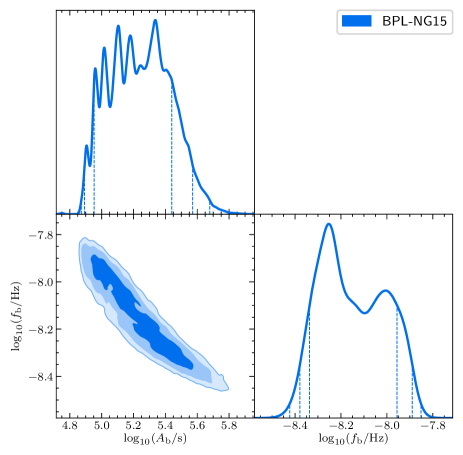
Figure 3: The lower left panel in this plot shows the $68\%$, $95\%$, and $99\%$ confidence levels of the $2$-dimensional posterior distribution for the parameters of the broken power-law fitting function: ${\rm log}_{10}(A_{\rm b}/{\rm s})$ and ${\rm log}_{10}(f_{\rm b}/{\rm Hz})$. The other two panels show the $1$-dimensional marginalized posterior distributions for these parameters. The dashed vertical lines in the plots for the $1$-dimensional distributions indicate the $68\%$, $95\%$, and $99\%$ credible intervals. The uniform priors used in this analysis are: ${\rm log}_{10}(A_{\rm b}/{\rm s})\in[2.0,8.0]$ and ${\rm log}_{10}(f_{\rm b}/{\rm Hz})\in[-10.0,-6.0]$. We also assume Hellings & Downs correlations between the pulsars.

3.2 Early and late dark energy

Following the initial phase of DBI kination domination enhancing the GW spectrum (see Fig 2), the DBI Lorentz factor $\gamma$ returns to small values (see Fig 1). The subsequent scalar dynamics is smoothly matched to a second phase, mainly controlled by the potential terms of eq (2.8). The potential-dominated phase allows us to realize a scenario including both an early dark energy (EDE) epoch, as well a late dark energy (LDE) phase which explains the present day acceleration of the universe.

The scalar potential (2.8) has been recently considered in [41, 42] as a possible way to relax the so called $H_{0}$ tension in cosmology, via the injection of an early period of dark energy domination, driven by the scalar $\phi$, called early dark energy (EDE) (see [65, 66] for early EDE models). The $H_{0}$ tension refers to the discrepancy between local measurements of the Hubble parameter today from supernovae, and its inferred value from cosmic microwave background (CMB) measurements assuming the standard $\Lambda$CDM cosmological model (for recent reviews on the $H_{0}$ tension and solutions see [26, 27]. For recent reviews on EDE models see [67, 68]). As discussed in section 2, in our case the potential also includes an additional term, leading to a LDE domination driven by the axion [69]. In total, the potential expressed in terms of the dimensionless scalar field $\varphi$ can be written as (recall that the decay constants are dimensionless and given in Planck units):

$$V(\varphi)=V_{0_{\rm ede}}\left(1-\cos[\varphi/f_{1}]\right)^{3}+V_{0_{\rm de}}\left(1-\cos[\varphi/f_{2}]\right)\,.$$ (3.8)

The first term is responsible for the EDE epoch, and we select $V_{0_{\rm ede}}\sim{\rm eV}^{4}$; the second term leads to late time acceleration, hence $V_{0_{\rm de}}\sim(0.002\,{\rm eV})^{4}$. The axionic evolution controlled by the potential terms is preceded by the DBI kinetic evolution of section 3.1: the requirement of matching the two phases partially determines the parameters of the model, as in Table 2. Interestingly, this matching connects the early DBI kination phase which enhances the GW signal, to a later evolution contributing to the physics of the dark universe.

$V_{0_{\rm ede}}$	$V_{0_{\rm de}}$	$f_{1}$	$f_{2}$
$(6.32\times 10^{-10}\,{\rm GeV})^{4}$	$1.45247\times 10^{-47}\,{\rm GeV}^{4}$	$0.3569$	$0.1044$

Table 2: The values of the parameters in the scalar potential (3.8).

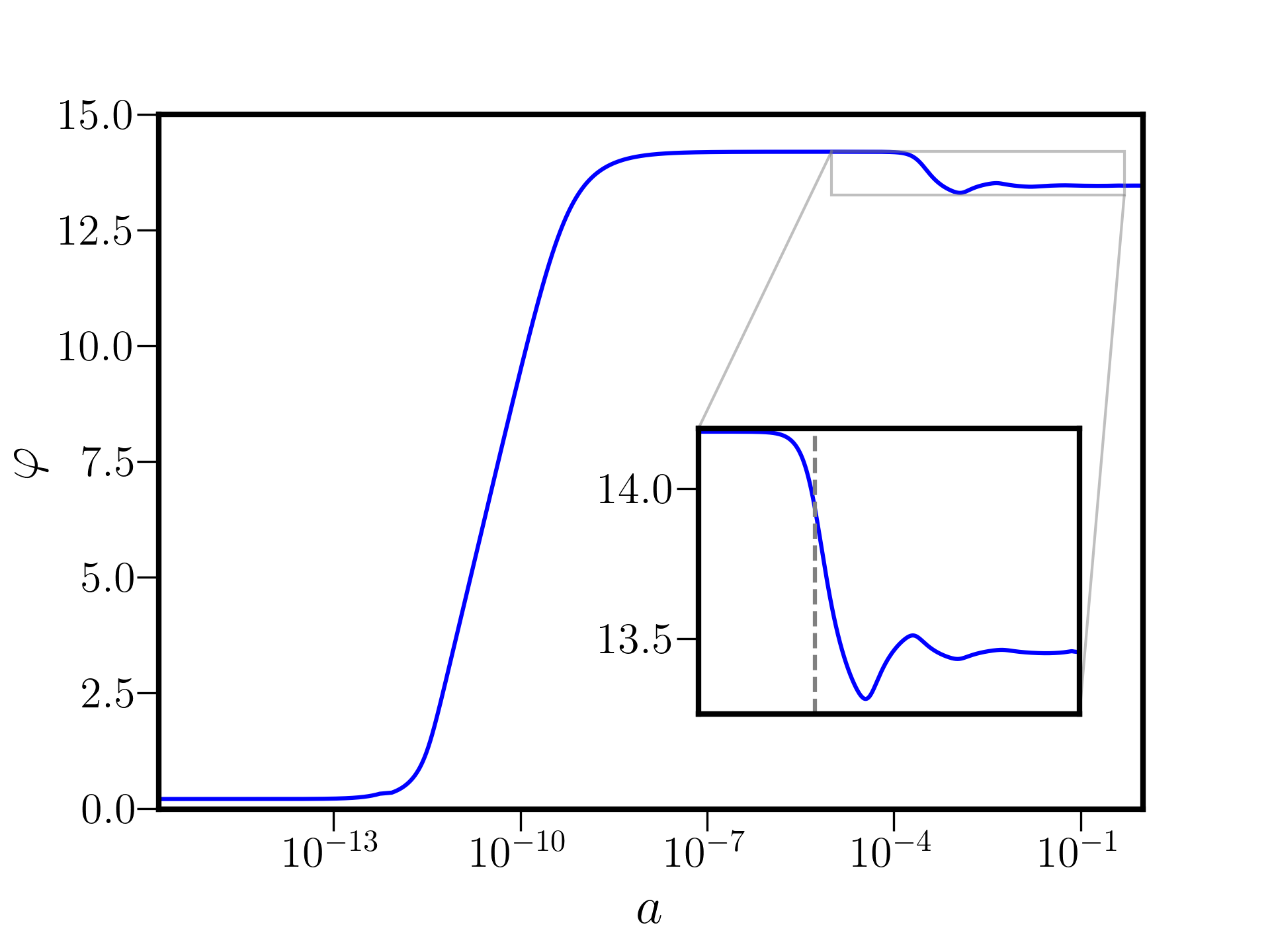
Figure 4: The evolution of the scalar field $\varphi$ as a function of the scale factor in our set-up. The initial conditions and parameter values can be found in Tables 1 and  2. In the inset, we have zoomed into the region where the field oscillates around the minimum of the EDE potential. The dashed vertical line in the inset corresponds to a redshift of $z\sim 10^{3.562}$, which is around the time when the fractional energy density of the EDE component reaches its maximum value (see Fig. 5 and associated discussions for more details).

The initial conditions for the field, its velocity, and the Hubble expansion rate are chosen as discussed in section 3.1. Once these are set, we have to choose values for the parameters describing the potential (3.8). Since the EDE energy density must decay faster than the energy density of matter or radiation, the value of $n$ is restricted to be $\geq 3$. In our analysis, we fix this value to be $n=3$. The other two parameters relevant for EDE, i.e. $V_{0_{\rm ede}}$ and $f_{1}$, are chosen such that we satisfy the two conditions that the EDE component contributes $\sim 12\%$ of the total energy density of the universe, and the maximum of the EDE energy density occurs around the time of matter-radiation equality. The parameters $V_{0_{\rm de}}$ and $f_{2}$ are similarly chosen such that the onset of LDE domination occurs recently and at the correct energy scale so as to account for the current accelerated expansion of the universe.

The value for the EDE decay constant $f_{1}$ turns out to be sub-Planckian, while we choose the value of the LDE decay constant $f_{2}$ as

$$f_{2}\simeq\frac{2q}{2m+1}\,f_{1}\,,$$ (3.9)

with $q,m$ being integers. The quantity $q$ is determined by the periodicity of the EDE potential, $2\pi f_{1}$, and the value of $\varphi$ is determined at an epoch where the DBI kinetic effects end. By choosing a sufficiently large $m$, the value of $f_{2}$ relevant for LDE can be made sufficiently small in Planck units potentially satisfying the constraints from the weak gravity conjecture for EDE [72]. For the values in Table 2 we have $q=6$ and we choose $m=20$.

Figure 4 shows the evolution of the scalar field as a function of the universe temperature, starting from the initial conditions after inflation of Table 1. During the initial epoch of DBI-kination, the field is unaffected by the potential. The axion potential becomes relevant at around $T\sim$ eV, where the field value remains frozen by the Hubble friction acting as a cosmological constant: this corresponds to the phase of EDE domination. In order to satisfy current constraints, and help in ameliorating the Hubble tension, the fractional energy density contributed by the EDE component,

$$f_{\rm EDE}(z)\equiv\frac{\rho_{\rm EDE}}{\rho_{T}}\,,$$ (3.10)

should not exceed values around $12\%$ (see e.g. [67, 68]). This requirement is satisfied in our set-up, see Fig 5. It would nevertheless be important to analyse in more detail whether our modified evolution equation is in agreement with current CMB constraints: this goes beyond the scope of this work, and we defer it to a separate study.

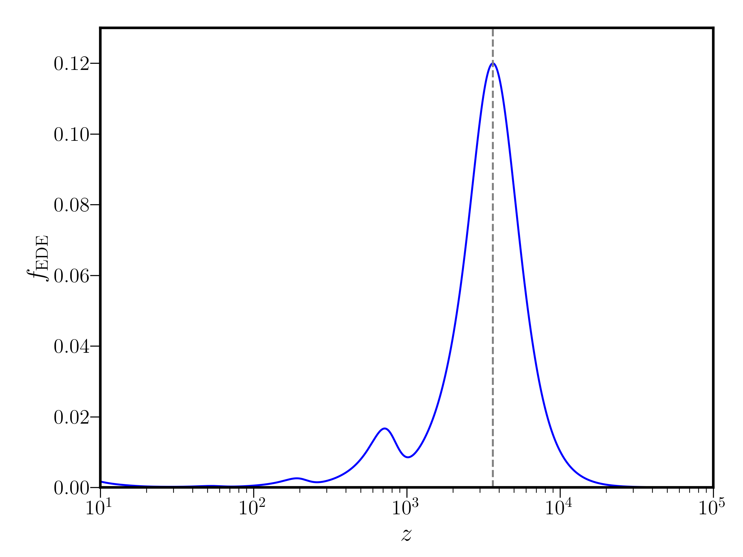
Figure 5: The fractional contribution of the EDE to the total energy density has been plotted as a function of redshift. It reaches a maximum value of $\sim 0.12$ around $\log_{10}z\sim 3.562$, which has been shown to help in relaxing the Hubble tension [73].

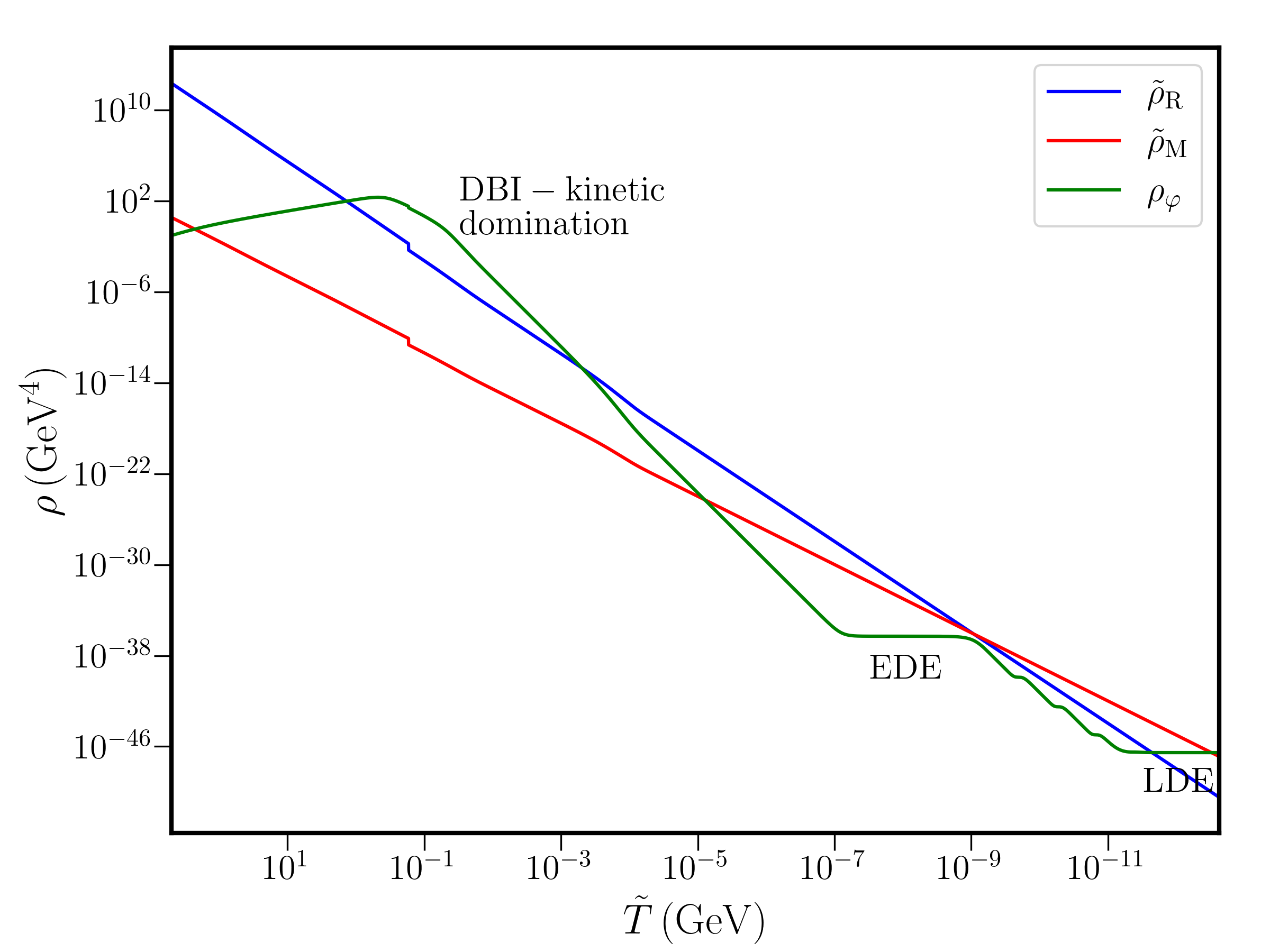
Figure 6: Plot of the different contributions to the energy density of the universe as a function of the universe temperature. The behaviour of the scalar field energy density at different temperatures illustrates the DBI kination epoch – the scalar energy density transiently dominates over the other energy densities at high temperatures – the EDE epoch – the scalar energy density is constant and subdominant at intermediate temperatures – and the LDE epoch – the scalar energy density returns to a constant value driving present-day acceleration.

As the temperature of the universe decreases, the axion field rolls to the minimum of the EDE potential, around which it oscillates until it feels the second LDE potential in eq (3.8). This leads to the current cosmological acceleration. In Figure 6 we plot the evolution of the separate contributions to the total energy density of the universe from radiation, matter, and the axion field. The figure shows three epochs driven by the D-brane axionic field: DBI kination, EDE, and LDE. During the first phase of DBI kination the scalar contribution briefly dominates the energy density; in the phase of EDE the scalar energy density is almost constant, and subdominant; in the last phase of LDE the scalar energy density is again constant, and eventually starts to dominate the total energy density.

4 Discussion

The recent detection of a stochastic GW background by several PTA collaborations raises the question of its origin. In this work we explored the possibility that it is sourced by cosmic inflation, a well-known source of primordial GW. The inflationary GW background amplitude is enhanced at PTA scales by a non-standard early cosmological evolution, driven by a kinetically-dominated scalar-tensor dynamics motivated by string theory. The resulting GW energy density has a distinctive broken power-law frequency profile, entering the PTA band with a peak amplitude consistent with the recent GW detections. Our framework – besides providing a possible explanation for the recent PTA results – also sheds light on other well-known cosmological problems. It provides a realization of an early dark energy scenario aimed to address the $H_{0}$ tension, and a late dark energy model which explains the current cosmological acceleration with no need of a cosmological constant.

Several questions are left for further exploring this connection between GW in the PTA band and the physics of the dark universe. It will be interesting to test in detail our specific broken power-law frequency profile for the GW energy density against the actual PTA data that are being currently released. It would also be important to develop more careful tests of the early dark energy scenario we propose, for example comparing it against constraints from CMB observations, to further restrict our parameter space. This analysis would require to modify existing CMB codes to accommodate the details of our set-up. Since the characteristic energy scale of the mechanism we propose is set around the scale of QCD transition, our scenario can have further consequences for the predictions of dark matter relic density and sterile neutrinos (see e.g. [14]). We leave some of these investigations to a forthcoming work.

Acknowledgments

We are partially funded by the STFC grant ST/T000813/1. For the purpose of open access, the authors have applied a Creative Commons Attribution licence to any Author Accepted Manuscript version arising.

Appendix A Determining the initial condition for $H$

In this appendix we briefly describe how we fix the initial conditions for the Hubble parameter in our analysis. We define the Hubble parameter in the standard $\Lambda$CDM scenario as

$$H_{\Lambda{\rm CDM}}^{2}=\frac{\kappa^{2}}{3}\,\left(\tilde{\rho}_{\rm R}+\tilde{\rho}_{\rm M}+\tilde{\rho}_{\Lambda}\right)=\frac{\kappa^{2}}{3}\,\tilde{\rho}_{\rm bg}.$$ (A.1)

The Hubble parameter in the disformal DBI case can be expressed as

$$H^{2} =\frac{\kappa^{2}}{3}\,\left(\rho_{{}_{\varphi}}+\rho_{\rm bg}\right)$$

$$=\frac{\kappa^{2}}{3\,B}\,\left(\,\gamma\,\tilde{\rho_{\rm bg}}+V\right).$$ (A.2a)

Using the expression (2.14), we can write

$$H^{2}\left[1-\frac{\gamma^{2}\,\varphi_{{}_{N}}^{2}}{3\,(\gamma+1)}\right]=\frac{\kappa^{2}}{3}\,\left(\,\gamma\,\tilde{\rho_{\rm bg}}+V\right).$$ (A.3)

Substituting the relation (2.13), we get the following quartic equation in $\gamma$:

$$\gamma^{4}\left(M^{-4}\,\varphi_{{}_{N}}^{2}\,\,\tilde{\rho}_{\rm bg}+\varphi_{{}_{N}}^{2}\right) + \gamma^{3}\left(M^{-4}\,\varphi_{{}_{N}}^{2}\,V-3\,\right)+\gamma^{2}\left(M^{-4}\,\varphi_{{}_{N}}^{2}\,\,\tilde{\rho}_{\rm bg}-3\,-\,\varphi_{{}_{N}}^{2}\right)$$ (A.4)

$$+ \gamma\left(M^{-4}\,\varphi_{{}_{N}}^{2}\,V+3\,\right)+3\,=0.$$

This equation can be solved to obtain four initial values of $\gamma$ for a given set of initial conditions. For our system, we choose the value of $\gamma_{i}$ to be real and of order one. With this choice of $\gamma_{i}$, we can then obtain the value of $H_{i}$ from the relation (2.13).

References

- [1] L. P. Grishchuk, Amplification of gravitational waves in an istropic universe, Zh. Eksp. Teor. Fiz. 67 (1974) 825–838.
- [2] A. A. Starobinsky, Spectrum of relict gravitational radiation and the early state of the universe, JETP Lett. 30 (1979) 682–685.
- [3] V. A. Rubakov, M. V. Sazhin, and A. V. Veryaskin, Graviton Creation in the Inflationary Universe and the Grand Unification Scale, Phys. Lett. B 115 (1982) 189–192.
- [4] R. Fabbri and M. d. Pollock, The Effect of Primordially Produced Gravitons upon the Anisotropy of the Cosmological Microwave Background Radiation, Phys. Lett. B 125 (1983) 445–448.
- [5] L. F. Abbott and M. B. Wise, Constraints on Generalized Inflationary Cosmologies, Nucl. Phys. B 244 (1984) 541–548.
- [6] M. R. Haque, D. Maity, T. Paul, and L. Sriramkumar, Decoding the phases of early and late time reheating through imprints on primordial gravitational waves, Phys. Rev. D 104 (2021), no. 6 063513, [arXiv:2105.09242].
- [7] A. Ashoorioon, K. Rezazadeh, and A. Rostami, NANOGrav signal from the end of inflation and the LIGO mass and heavier primordial black holes, Phys. Lett. B 835 (2022) 137542, [arXiv:2202.01131].
- [8] S.-Y. Guo, M. Khlopov, X. Liu, L. Wu, Y. Wu, and B. Zhu, Footprints of Axion-Like Particle in Pulsar Timing Array Data and JWST Observations, arXiv:2306.17022.
- [9] M. Giovannini, Gravitational waves constraints on postinflationary phases stiffer than radiation, Phys. Rev. D 58 (1998) 083504, [hep-ph/9806329].
- [10] L. A. Boyle and A. Buonanno, Relating gravitational wave constraints from primordial nucleosynthesis, pulsar timing, laser interferometers, and the CMB: Implications for the early Universe, Phys. Rev. D 78 (2008) 043531, [arXiv:0708.2279].
- [11] L. A. Boyle and P. J. Steinhardt, Probing the early universe with inflationary gravitational waves, Phys. Rev. D 77 (2008) 063504, [astro-ph/0512014].
- [12] P. Salati, Quintessence and the relic density of neutralinos, Phys. Lett. B 571 (2003) 121–131, [astro-ph/0207396].
- [13] R. Catena, N. Fornengo, A. Masiero, M. Pietroni, and F. Rosati, Dark matter relic abundance and scalar - tensor dark energy, Phys. Rev. D 70 (2004) 063519, [astro-ph/0403614].
- [14] G. B. Gelmini, J.-H. Huh, and T. Rehagen, Asymmetric dark matter annihilation as a test of non-standard cosmologies, JCAP 08 (2013) 003, [arXiv:1304.3679].
- [15] A. B. Lahanas, N. E. Mavromatos, and D. V. Nanopoulos, Dilaton and off-shell (non-critical string) effects in Boltzmann equation for species abundances, PMC Phys. A 1 (2007) 2, [hep-ph/0608153].
- [16] C. Pallis, Cold Dark Matter in non-Standard Cosmologies, PAMELA, ATIC and Fermi LAT, Nucl. Phys. B 831 (2010) 217–247, [arXiv:0909.3026].
- [17] B. Dutta, E. Jimenez, and I. Zavala, Dark Matter Relics and the Expansion Rate in Scalar-Tensor Theories, JCAP 06 (2017) 032, [arXiv:1612.05553].
- [18] B. Dutta, E. Jimenez, and I. Zavala, D-brane Disformal Coupling and Thermal Dark Matter, Phys. Rev. D 96 (2017), no. 10 103506, [arXiv:1708.07153].
- [19] D. Chowdhury, G. Tasinato, and I. Zavala, The rise of the primordial tensor spectrum from an early scalar-tensor epoch, JCAP 08 (2022), no. 08 010, [arXiv:2204.10218].
- [20] NANOGrav Collaboration, G. Agazie et al., The NANOGrav 15-year Data Set: Evidence for a Gravitational-Wave Background, Astrophys. J. Lett. 951 (2023), no. 1 [arXiv:2306.16213].
- [21] D. J. Reardon et al., Search for an isotropic gravitational-wave background with the Parkes Pulsar Timing Array, Astrophys. J. Lett. 951 (2023), no. 1 [arXiv:2306.16215].
- [22] J. Antoniadis et al., The second data release from the European Pulsar Timing Array III. Search for gravitational wave signals, arXiv:2306.16214.
- [23] H. Xu et al., Searching for the Nano-Hertz Stochastic Gravitational Wave Background with the Chinese Pulsar Timing Array Data Release I, Res. Astron. Astrophys. 23 (2023), no. 7 075024, [arXiv:2306.16216].
- [24] NANOGrav Collaboration, A. Afzal et al., The NANOGrav 15-year Data Set: Search for Signals from New Physics, Astrophys. J. Lett. 951 (2023), no. 1 [arXiv:2306.16219].
- [25] J. Antoniadis et al., The second data release from the European Pulsar Timing Array: V. Implications for massive black holes, dark matter and the early Universe, arXiv:2306.16227.
- [26] E. Di Valentino, O. Mena, S. Pan, L. Visinelli, W. Yang, A. Melchiorri, D. F. Mota, A. G. Riess, and J. Silk, In the realm of the Hubble tension—a review of solutions, Class. Quant. Grav. 38 (2021), no. 15 153001, [arXiv:2103.01183].
- [27] N. Schöneberg, G. Franco Abellán, A. Pérez Sánchez, S. J. Witte, V. Poulin, and J. Lesgourgues, The H0 Olympics: A fair ranking of proposed models, Phys. Rept. 984 (2022) 1–55, [arXiv:2107.10291].
- [28] J. D. Bekenstein, The Relation between physical and gravitational geometry, Phys. Rev. D 48 (1993) 3641–3647, [gr-qc/9211017].
- [29] K. Rezazadeh, A. Ashoorioon, and D. Grin, Cascading Dark Energy, arXiv:2208.07631.
- [30] M. Cicoli, J. P. Conlon, A. Maharana, S. Parameswaran, F. Quevedo, and I. Zavala, String Cosmology: from the Early Universe to Today, arXiv:2303.04819.
- [31] T. Koivisto, D. Wills, and I. Zavala, Dark D-brane Cosmology, JCAP 06 (2014) 036, [arXiv:1312.2597].
- [32] J. Sakstein, Disformal Theories of Gravity: From the Solar System to Cosmology, JCAP 12 (2014) 012, [arXiv:1409.1734].
- [33] C. van de Bruck and E. M. Teixeira, Dark D-Brane Cosmology: from background evolution to cosmological perturbations, Phys. Rev. D 102 (2020), no. 10 103503, [arXiv:2007.15414].
- [34] J. Polchinski, Tasi lectures on D-branes, in Theoretical Advanced Study Institute in Elementary Particle Physics (TASI 96): Fields, Strings, and Duality, pp. 293–356, 11, 1996. hep-th/9611050.
- [35] Z. Kenton and S. Thomas, D-brane Potentials in the Warped Resolved Conifold and Natural Inflation, JHEP 02 (2015) 127, [arXiv:1409.1221].
- [36] D. Chakraborty, R. Chiovoloni, O. Loaiza-Brito, G. Niz, and I. Zavala, Fat inflatons, large turns and the -problem, JCAP 01 (2020) 020, [arXiv:1908.09797].
- [37] P. Candelas and X. C. de la Ossa, Comments on Conifolds, Nucl. Phys. B342 (1990) 246–268.
- [38] L. A. Pando Zayas and A. A. Tseytlin, 3-branes on resolved conifold, JHEP 11 (2000) 028, [hep-th/0010088].
- [39] I. R. Klebanov and A. Murugan, Gauge/Gravity Duality and Warped Resolved Conifold, JHEP 03 (2007) 042, [hep-th/0701064].
- [40] D. Baumann, A. Dymarsky, S. Kachru, I. R. Klebanov, and L. McAllister, D3-brane Potentials from Fluxes in AdS/CFT, JHEP 06 (2010) 072, [arXiv:1001.5028].
- [41] V. Poulin, T. L. Smith, D. Grin, T. Karwal, and M. Kamionkowski, Cosmological implications of ultralight axionlike fields, Phys. Rev. D 98 (2018), no. 8 083525, [arXiv:1806.10608].
- [42] V. Poulin, T. L. Smith, T. Karwal, and M. Kamionkowski, Early Dark Energy Can Resolve The Hubble Tension, Phys. Rev. Lett. 122 (2019), no. 22 221301, [arXiv:1811.04083].
- [43] N. Kaloper and L. Sorbo, Of pngb quintessence, JCAP 04 (2006) 007, [astro-ph/0511543].
- [44] Planck Collaboration, P. A. R. Ade et al., Planck 2015 results. XIV. Dark energy and modified gravity, Astron. Astrophys. 594 (2016) A14, [arXiv:1502.01590].
- [45] T. Damour and K. Nordtvedt, Tensor - scalar cosmological models and their relaxation toward general relativity, Phys. Rev. D 48 (1993) 3436–3450.
- [46] P. G. Ferreira and M. Joyce, Cosmology with a primordial scaling field, Phys. Rev. D 58 (1998) 023503, [astro-ph/9711102].
- [47] K. Redmond, A. Trezza, and A. L. Erickcek, Growth of Dark Matter Perturbations during Kination, Phys. Rev. D 98 (2018), no. 6 063504, [arXiv:1807.01327].
- [48] R. T. Co, D. Dunsky, N. Fernandez, A. Ghalsasi, L. J. Hall, K. Harigaya, and J. Shelton, Gravitational wave and CMB probes of axion kination, JHEP 09 (2022) 116, [arXiv:2108.09299].
- [49] Y. Gouttenoire, G. Servant, and P. Simakachorn, Kination cosmology from scalar fields and gravitational-wave signatures, arXiv:2111.01150.
- [50] N. Bernal, A. Ghoshal, F. Hajkarim, and G. Lambiase, Primordial Gravitational Wave Signals in Modified Cosmologies, JCAP 11 (2020) 051, [arXiv:2008.04959].
- [51] Y. Watanabe and E. Komatsu, Improved Calculation of the Primordial Gravitational Wave Spectrum in the Standard Model, Phys. Rev. D 73 (2006) 123515, [astro-ph/0604176].
- [52] K. Saikawa and S. Shirai, Primordial gravitational waves, precisely: The role of thermodynamics in the Standard Model, JCAP 05 (2018) 035, [arXiv:1803.01038].
- [53] N. Bernal and F. Hajkarim, Primordial Gravitational Waves in Nonstandard Cosmologies, Phys. Rev. D 100 (2019), no. 6 063502, [arXiv:1905.10410].
- [54] BICEP, Keck Collaboration, P. A. R. Ade et al., Improved Constraints on Primordial Gravitational Waves using Planck, WMAP, and BICEP/Keck Observations through the 2018 Observing Season, Phys. Rev. Lett. 127 (2021), no. 15 151301, [arXiv:2110.00483].
- [55] M. Kamionkowski, A. Kosowsky, and M. S. Turner, Gravitational radiation from first order phase transitions, Phys. Rev. D 49 (1994) 2837–2851, [astro-ph/9310044].
- [56] NANOGrav Collaboration, G. Agazie et al., The NANOGrav 15 yr Data Set: Detector Characterization and Noise Budget, Astrophys. J. Lett. 951 (2023), no. 1 L10, [arXiv:2306.16218].
- [57] The NANOGrav Collaboration, Noise Spectra and Stochastic Background Sensitivity Curve for the NG15-year Dataset, .
- [58] E. Thrane and J. D. Romano, Sensitivity curves for searches for gravitational-wave backgrounds, Phys. Rev. D 88 (2013), no. 12 124032, [arXiv:1310.5300].
- [59] K. Schmitz, New Sensitivity Curves for Gravitational-Wave Signals from Cosmological Phase Transitions, JHEP 01 (2021) 097, [arXiv:2002.04615].
- [60] NANOGrav Collaboration, Z. Arzoumanian et al., The NANOGrav 12.5 yr Data Set: Search for an Isotropic Stochastic Gravitational-wave Background, Astrophys. J. Lett. 905 (2020), no. 2 L34, [arXiv:2009.04496].
- [61] A. Mitridate and D. Wright, PTArcade, .
- [62] A. Mitridate, D. Wright, R. von Eckardstein, T. Schröder, J. Nay, K. Olum, K. Schmitz, and T. Trickle, PTArcade, arXiv:2306.16377.
- [63] W. G. Lamb, S. R. Taylor, and R. van Haasteren, The Need For Speed: Rapid Refitting Techniques for Bayesian Spectral Characterization of the Gravitational Wave Background Using PTAs, arXiv:2303.15442.
- [64] N. Kitajima and T. Takahashi, Stochastic gravitational wave background from early dark energy, arXiv:2306.16896.
- [65] C. Wetterich, Phenomenological parameterization of quintessence, Phys. Lett. B 594 (2004) 17–22, [astro-ph/0403289].
- [66] M. Doran and G. Robbers, Early dark energy cosmologies, JCAP 06 (2006) 026, [astro-ph/0601544].
- [67] M. Kamionkowski and A. G. Riess, The Hubble Tension and Early Dark Energy, arXiv:2211.04492.
- [68] V. Poulin, T. L. Smith, and T. Karwal, The Ups and Downs of Early Dark Energy solutions to the Hubble tension: a review of models, hints and constraints circa 2023, arXiv:2302.09032.
- [69] J. E. Kim and H. P. Nilles, A Quintessential axion, Phys. Lett. B 553 (2003) 1–6, [hep-ph/0210402].
- [70] E. McDonough and M. Scalisi, Towards Early Dark Energy in String Theory, arXiv:2209.00011.
- [71] M. Cicoli, M. Licheri, R. Mahanta, E. McDonough, F. G. Pedro, and M. Scalisi, Early Dark Energy in Type IIB String Theory, JHEP 06 (2023) 052, [arXiv:2303.03414].
- [72] T. Rudelius, Constraints on early dark energy from the axion weak gravity conjecture, JCAP 01 (2023) 014, [arXiv:2203.05575].
- [73] J. C. Hill, E. McDonough, M. W. Toomey, and S. Alexander, Early dark energy does not restore cosmological concordance, Phys. Rev. D 102 (2020), no. 4 043507, [arXiv:2003.07355].