Real-time Likelihood Methods for Improved $\gamma$-ray Transient Detection and Localization

Abstract

We present a maximum likelihood (ML) algorithm that is fast enough to detect $\gamma$-ray transients in real time on low-performance processors often used for space applications. We validate the routine with simulations and find that, relative to algorithms based on excess counts, the ML method is nearly twice as sensitive, allowing detection of 240–280% more short $\gamma$-ray bursts. We characterize a reference implementation of the code, estimating its computational complexity and benchmarking it on a range of processors. We exercise the reference implementation on archival data from the Fermi Gamma-ray Burst Monitor (GBM), verifying the sensitivity improvements. In particular, we show that the ML algorithm would have detected GRB 170817A even if it had been nearly four times fainter. We present an ad hoc but effective scheme for discriminating transients associated with background variations. We show that the on-board localizations generated by ML are accurate, but that refined off-line localizations require a detector response matrix with about ten times finer resolution than is current practice. Increasing the resolution of the GBM response matrix could substantially reduce the few-degree systematic uncertainty observed in the localizations of bright bursts.

1 Introduction

The prompt emission from $\gamma$-ray bursts (GRBs) is typically concentrated between 100 keV and 1 MeV (von Kienlin et al., 2020; Poolakkil et al., 2021) and varies in duration from $<$2 s (short GRBs, Kouveliotou et al., 1993) to minutes (long GRBs), to hours (rare ultra-long GRBs, Levan et al., 2014). These soft $\gamma$ rays primarily Compton scatter, limiting detection technologies. Wideband Compton telescopes reconstruct the photon interaction and provide a wide field-of-view and modest effective area, but they require very high-resolution, expensive detector elements and readout systems (e.g. Tomsick et al., 2019; McEnery et al., 2019). Coded masks enable indirect imaging up to 100–200 keV (when the mask becomes transparent) with modest field-of-view and angular resolution: the Burst Alert Telescope is capable of providing GRB localizations to $<$1’ (Barthelmy et al., 2005) in a 30^∘ field-of-view. Laue lenses allow direct focusing via coherent Bragg scattering (Frontera & von Ballmoos, 2010), but their bulk, cost, and narrow field-of-view are impractical for all-sky monitoring.

Scintillating crystals provide effective stopping power over a wide energy range and can be read out with simple electronics. Doped NaI and CsI can be grown to large sizes, offering exceptional sensitivity-to-cost ratio, and detectors based on these crystals have been widely used for $\gamma$-ray transient detection. The Vela nuclear test monitoring system used CsI detectors in its serendipitous discovery of GRBs (Klebesadel et al., 1973). The pioneering (Meegan et al., 1992) Burst and Transient Source Experiment (BATSE) on the Compton Gamma-Ray Observatory used very large NaI scintillators that were viewed from the side with photomultiplier tubes. The Gamma-ray Burst Monitor (GBM) on the Fermi Gamma-Ray Space Telescope uses much smaller NaI pucks with Be windows read from the large face to maximize light yield, enabling a particularly low ($\sim$10 keV) threshold (Meegan et al., 2009). Future experiments like Glowbug (Woolf et al., 2022) and Starburst (Kocevski, 2022) will use large, thin crystals read out from the edge with silicon photomultipliers (SiPMs, Mitchell et al., 2021) to achieve very high sensitivity in a compact, low-voltage, low-cost design.

Scintillators have fast scintillation and readout times, typically $\lesssim$1 $\mu$s, enabling photon counting but providing no position information. Instead, comparing rates between two detectors with differing incidence angles constrains the source position to a fuzzy great circle. Additional detector pairs provide further constraints and reduce the uncertainty, and many pairs yield a localization that is well-described as a single point with a gaussian-distributed uncertainty. Increasing the signal-to-background ratio further reduces the uncertainty, allowing for designs with a few large facets (Glowbug) or many smaller facets (GBM) to produce comparable localizing power.

Scintillators also provide no intrinsic discrimination of background events, e.g. from energetic particles trapped in earth’s magnetosphere or $\gamma$ rays produced by internal radioactivation. Time-dependent background variations can mimic a $\gamma$-ray transient, so a detector system must first recognize it, i.e. trigger. Triggers often initiate resource-intensive processes, such as re-pointing the spacecraft or downlinking a large volume of data for offline analysis. Thus, trigger criteria and algorithms must be carefully tuned to provide sensitivity to transients while minimizing false positives. GBM provides one example of an effective on-board trigger scheme (Meegan et al., 2009): it autonomously measures the background rate in each NaI detector, averages excess counts over a range of timescales, and triggers when two or more detectors register a $>$4.5$\sigma$ excess.

Large SiPM-read crystals, the availability of cheap commercial SmallSat spacecraft buses, and rideshare launch opportunities mean it is now possible to launch $\gamma$-ray transient detectors with the performance of heritage instruments at a fraction of the cost. Such detectors will have limited telemetry bandwidth, so a sensitive trigger is required to maximize the scientific merit of the data that are downlinked. For example, the short GRBs accompanying neutron star mergers are expected to be faint because future gravitational wave detectors will detect more distant mergers and because the jetted emission will not generally point towards earth. GRB 170817A was exceptionally close but was only 7% over the GBM trigger threshold (Goldstein et al., 2017).

In this work, we propose to improve trigger sensitivity and efficiency by using maximum likelihood (ML) for the on-board detection and localization of GRBs and other $\gamma$-ray transients. ML methods are already used for offline analysis of GRB spectra and positions (Berlato et al., 2019; Goldstein et al., 2020) and for post facto detection (Blackburn et al., 2015; Kocevski et al., 2018). We show that such methods are capable of running in real-time on the low-power, low-performance processors typically used for space applications and that they can detect transients that are half as bright as those detectable with rate-based triggers. Moreover, ML links detection and localization, so a coarse position is available immediately upon detection, enabling very low-latency alerts. The same framework can be used to rapidly refine the localization. Finally, ML methods can be tuned to different source classes, including backgrounds, allowing efficient filtering of desired transients.

In the next section, we develop the formalism for ML detection and localization with scintillator detectors and show that some simple approximations yield fast but reliable estimates of transient significance. In $3, we use Monte Carlo simulations of a GBM-like dataset to validate the ML estimators for detection and localization and to estimate the threshold transient flux, allowing an estimate of the relative sensitivity. We describe the computational performance of a reference implementation in §4 in theory and as benchmarked on relevant hardware. We characterize the algorithmic performance in §5, demonstrating both sensitivity to bona fide GRBs and an effective method of reducing false triggers from particle backgrounds. We consider the accuracy of both coarse and follow-up localization in §6, finding that the reliability depends strongly on the spatial resolution of the detector response matrix. Finally, we conclude with a summary of the results and a discussion of potential new applications enabled by the method in §7.

2 Fast likelihood methods

$\gamma$-ray/$e^{-}$ interactions in a scintillator release a pulse of optical light that is collected, amplified, and measured. For a thick scintillator, the incident energy $E^{\prime}$ is entirely converted to a pulse height $E$ proportional to $E^{\prime}$ with a spectral resolution of order 5%. For thin crystals/higher energies, scattered photons and electrons may escape, yielding $E$ possibly much less than $E^{\prime}$. The conversion efficiency (effective area) also drops with increasing energy until pair production begins.

The effective area and the energy redistribution can be encapsulated in a response matrix (RM) that converts $\gamma$ rays from a distant source incident at angle $\Omega$ with spectral flux density $F(E^{\prime})$ ($\mathrm{ph}\,\mathrm{keV}^{-1}\,\mathrm{s}^{-1}\,\mathrm{cm}^{-2}$) into an observed counts spectrum $N(E)$ ($\mathrm{ph}\,\mathrm{keV}^{-1}\,\mathrm{s}^{-1}$):

$$N(E)=\int_{0}^{\infty}dE^{\prime}R(E,E^{\prime},\Omega)F(E^{\prime},\Omega).$$ (1)

The RM is typically estimated with Monte Carlo simulations and particle transport codes and tabulated as a matrix, $R_{lijq}$: the response to a pixel centered on $\Omega_{l}$, for a detector with index $i$, averaged over observed/measured energy channel centered on $E_{j}$, averaged over incident energy channel centered on $E_{q}$. $R$ typically depends on time, and a spacecraft pointing history relates source coordinates to instrument coordinates. We adopt a source model with a background rate ($b_{ij}$) for each detector element ($i$) and energy channel ($j$) and a point source at position $\Omega_{l}$ with spectrum $F_{k}(E)$ ($k$ just labels this spectral shape). The predicted counts per unit time are then

$$\lambda_{klij}= \ b_{ij}+\alpha_{kl}\sum_{q}R_{lijq}F_{k}(E_{q})$$ (2)

$$\equiv \ b_{ij}+\alpha_{kl}F_{klij}.$$ (3)

The second line re-expresses the convolution of the source spectrum with $R$ as a fiducial “template” $F$ for the observed counts. The fiducial template is scaled by the source amplitude $\alpha_{kl}$ to produce the final counts prediction. The observed counts $n_{ij}$ follow a Poisson distribution, so an estimator for the source amplitude $\hat{\alpha}_{kl}$ can be obtained by maximizing the log likelihood

$$\log\mathcal{L}(\alpha_{kl})=\sum_{i=1}^{\mathrm{N_{det}}}\sum_{j=1}^{\mathrm{N_{chan}}}n_{ij}\log\left(b_{ij}+\alpha_{kl}F_{klij}\right)-b_{ij}-\alpha_{kl}F_{klij}.$$ (4)

Source significance can be estimated with the log likelihood ratio test statistic $\mathrm{TS}\equiv 2\times\left[\log\mathcal{L}(\hat{\alpha_{kl}})-\log\mathcal{L}(0)\right]$. Wilks (1938) shows that $\mathrm{TS}$ asymptotically follows a $\chi^{2}_{1}$ distribution. By appeal to the Cramér-Rao bound, this is also the most sensitive detection statistic.

For detection, we must scan over possible source positions and spectral shapes, obtaining sets of $\alpha_{kl}$ and $\mathrm{TS}(\alpha_{kl})$ for each time interval of interest. These evaluations are expensive, and a fast method is critical for real-time applications. We can focus on transients that are near-threshold, because bright transients will produce obvious signals. Thus, we write

$$\log\mathcal{L}(\alpha_{kl})= \ \sum_{i=1}^{\mathrm{N_{det}}}\sum_{j=1}^{\mathrm{N_{chan}}}n_{ij}\log\left(1+\alpha_{kl}F_{klij}/b_{ij}\right)-b_{ij}-\alpha_{kl}F_{klij}+\mathrm{const.}$$ (5)

$$\equiv \ \sum_{i=1}^{\mathrm{N_{det}}}\sum_{j=1}^{\mathrm{N_{chan}}}\left[n_{ij}\log\left(1+\alpha_{kl}t_{klij}\right)\right]-B-\alpha_{kl}F_{kl},$$ (6)

where we have defined $t$ as the ratio of source to background counts and have defined data-integrated quantities $B$ and $F_{kl}$. Taylor expanding the logarithm yields

$$\log\mathcal{L}(\alpha_{kl})= \ \sum_{i=1}^{\mathrm{N_{det}}}\sum_{j=1}^{\mathrm{N_{chan}}}\left[n_{ij}\left(\alpha_{kl}t_{klij}-\frac{1}{2}(\alpha_{kl}t_{klij})^{2}+\frac{1}{3}(\alpha_{kl}t_{klij})^{3}+\dots\right)\right]-B-\alpha_{kl}F_{kl}$$ (7)

$$\equiv \ \alpha_{kl}\langle NT_{kl}\rangle-\frac{\alpha_{kl}^{2}}{2}\langle NT_{kl}^{2}\rangle+\frac{\alpha_{kl}^{3}}{3}\langle NT_{kl}^{3}\rangle+\dots-B-\alpha_{kl}F_{kl},$$ (8)

where quantities like $\langle NT\rangle$ are moments of the data (counts) weighted by $t$. Differentiating and discarding remaining terms $\mathcal{O}(\alpha^{2})$ and higher yields the first-order estimator

$$\hat{\alpha}_{1kl}=\frac{\langle NT_{kl}\rangle-F_{kl}}{\langle NT_{kl}^{2}\rangle},$$ (9)

with $F_{l}$ now denoting the sum of all predicted counts. Inserting this estimator into the likelihood ratio test statistic and discarding terms $\mathcal{O}(\alpha^{3})$ yields the simple first-order estimator

$$\mathrm{TS}_{1}(\hat{\alpha}_{1kl})=\hat{\alpha}_{1kl}^{2}\langle NT_{kl}^{2}\rangle=\frac{\left(\langle NT_{kl}\rangle-F_{kl}\right)^{2}}{\langle NT_{kl}^{2}\rangle}$$ (10)

As we show below, it is helpful to consider a higher-order estimator formed from $\hat{\alpha}_{1kl}$ and the $\mathcal{O}(\alpha^{3})$ terms in Eq. 8:

$$\mathrm{TS}_{2}(\hat{\alpha}_{1kl})=\mathrm{TS}_{1}(\hat{\alpha}_{1kl})+\frac{2}{3}\hat{\alpha}_{1kl}^{3}\langle NT_{kl}^{3}\rangle$$ (11)

This expression neglects higher-order corrections to $\hat{\alpha}_{1kl}$, because (1) doing so requires choosing the correct solution to a quadratic equation and (2) the larger error is in the evaluation of $\mathrm{TS}$, so this simple correction is effective.

These expressions are summed over observed energy, but it is also useful to consider the estimators for each energy channel. Finally, we note that these expressions can be used to iteratively obtain the full maximum likelihood estimator $\hat{\alpha}_{kl}$ and hence the exact TS, which we denote $\mathrm{TS_{e}}(\hat{\alpha}_{kl})$.

Thus, a real-time, maximum likelihood based technique for transient detection (and localization) is as follows: (1) group events into time bins, e.g. 64 ms, 2,048 ms, …; (2) evaluate the approximate TS (TS₁ or TS₂) over a set of pixels corresponding to possible transient positions (unocculted space for GRBs, towards the nadir for terrestrial $\gamma$-ray flashes, etc.); (3) assess the significance of any large values to evaluate trigger criteria. We discuss the practical and efficient implementation of this approach further in §4. However, we first illustrate general properties of the ML estimator on somewhat idealized data and compare it to existing real-time detection schemes.

Channel	Trigger	Emin	Emax	Bkg. Rate	Bkg. Std
	Channel	(keV)	(kev)	(evt s-1)	(evt $s^{-1}$)
0	0	30	50	161	20
1	1	50	82	117	7
2	1	82	135	99	5
3	1	135	223	73	6
4	1	223	367	42	3
5	2	367	606	26	2
6	2	606	1000	51	18
7	–	1000	2000	38	16

Table 1: Channel edges used in simulation and later GBM data analysis. Note that the last channel includes overflow events. The second column indicates which channels are used in the GBM-like counts excess trigger. The background event rate, averaged over the 12 NaI detectors, is given here for reference, as is the variation (standard deviation) over the detectors.

3 Calibration and Sensitivity

In order to determine the sensitivity of the likelihood method, it is first necessary to determine the distribution of the likelihood test statistic in the absence of a signal, and thus a false alarm rate for any non-stationary signal (GRBs or other transients). For a given false alarm rate, the threshold can be mapped to a sensitivity in terms of transient flux. We carry out this procedure with simulations.

3.1 Simulation Setup

Archival GBM data, with its high time resolution, is ideal for validating burst-detection algorithms. To evaluate performance with known signal and background characterists, we here simulate “GBM-like” data. First, from archival data we estimate the typical background $b_{ai}$ for each NaI detector in 8 energy channels (Table 1). The variation in rates over detectors is modest except at the highest energies.

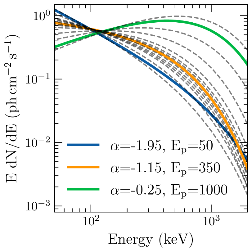
Figure 1: Spectral models for simulation and detection of GRBs. The colored lines represent three representative GRB spectra from Goldstein et al. (2020) and form a basis for detection, while the 12 black dashed lines form a basis for simulation.

Goldstein et al. (2020, hereafter G20) reported a set of three representative “Comptonized power law” models,

$$F(E)=N_{0}\left(\frac{E}{100\,\mathrm{keV}}\right)^{\alpha}\exp\left[-(2+\alpha)\frac{E}{E_{\mathrm{p}}}\right].$$ (12)

with parameters chosen to represent an unusually soft-spectrum GRB ($\alpha=-1.95$, $E_{\mathrm{p}}=50$ keV), a typical GRB ($\alpha=-1.15$, $E_{\mathrm{p}}=350$ keV), and an unusually hard-spectrum GRB ($\alpha=-0.25$, $E_{\mathrm{p}}=1000$ keV). We adopt these as our detection templates. However, to simulate a broader population, we have devised 12 “basis” spectra that do not overlap the G20 templates and cover a range around them (see Figure 1.) They are concentrated most densely around the “normal” model, and by choosing randomly between them, we can approximate drawing randomly from the population of GRBs. (The softest and hardest simulated spectra are even more extreme than G20 models, so in the simulations below we reduce the weight of these two templates by 50%.) The normalizations $N_{0}$ are chosen to give a 50–300 keV flux of 1 ph cm^-2 s^-1. We fold these basis spectral models through the GBM RM, obtained from the files distributed with gbmrsp. For consistency with the rest of our software, we resample the provided 272 spatial pixels to a 482-pixel icosahedral tessellation of the sky. The results predict the counts in 8 output channels (see Table 1 for boundaries) for each possible incidence direction.

To simulate a GRB—the alternative hypothesis—we choose one of the 12 spectral basis models and 482 incident directions at random, add the source rate to the background, scale the predicted rates by the duration $\delta t$, and draw Poisson random variables with the resulting mean, producing an array of $\mathrm{N_{det}}\times\mathrm{N_{chan}}$ ($12\times 8$) photon counts. (We use the 12 NaI detectors but neglect the 2 BGO detectors.) The null hypothesis is obtained in the same way but with zero source contribution.

3.2 Calibrating the Test Statistic

For each simulated data set, we evaluate the TS for the three G20 templates and for the 482 incident directions. (We reiterate that the simulation and detection templates are different.) We first examined the null hypothesis and found that the distribution of TS for a single template/pixel follows the expected asymptotic distribution ($\chi^{2}_{1}$) almost perfectly, even for short time windows ($\delta t=$64 ms) with typically only a few counts in each channel. However, the detection statistic is the maximum TS over pixels and templates, for which the distribution is not known. Furthermore, the sample values of TS are not independent because of finite angular resolution and because the GRB templates are not orthogonal. (The extent to which the pixels over- or undersample the angular resolution depends on the brightness of a given burst. Thus the distribution of the TS in the alternative hypothesis will in general be even more complicated.)

All of this means that the significance of any apparently-large TS must be calibrated with simulations. Fortunately, because the null distribution of TS does not depend on the time window $\delta t$, we can calibrate TS universally simply by simulating many realization of the null distribution ($\alpha\rightarrow 0$) and calculating the maximum TS over the pixels and templates, in this specific case, $3\times 482=1446$ values.

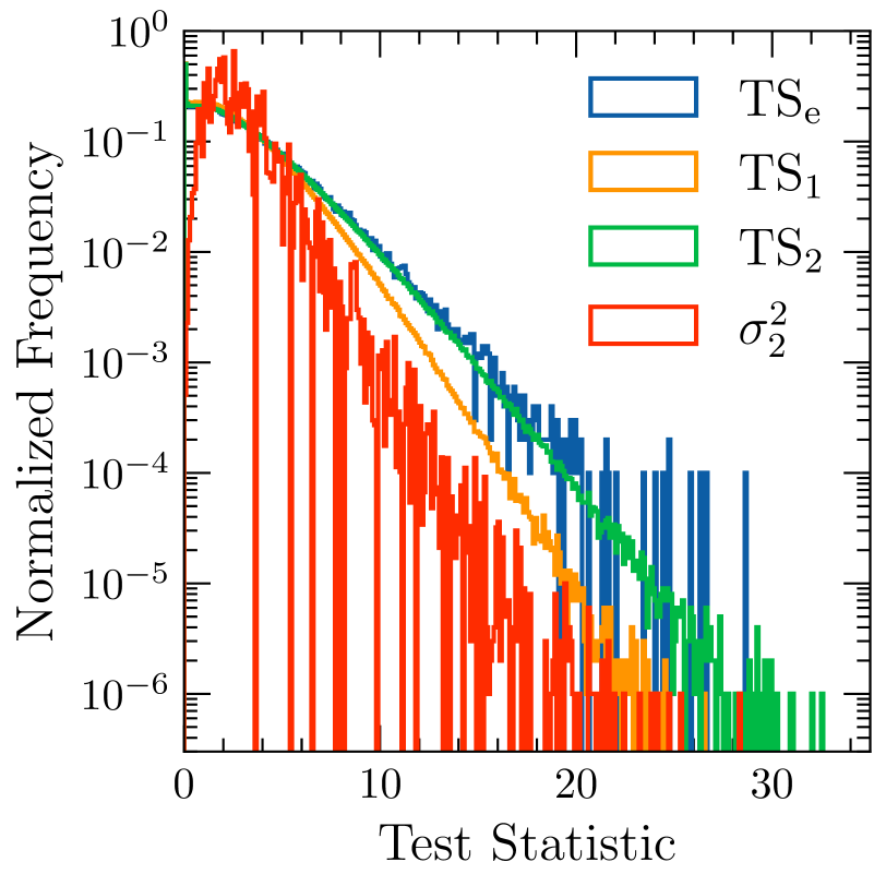
Figure 2: The maximum TS from a scan over 482 possible incident directions and 3 trial template spectra from simulations of the null hypothesis, i.e. background only. $\sigma_{2}$ is the Poisson significance of the third highest rate excess in the 12 detectors. There are $10^{7}$ realizations of TS₁, TS₂, and $\sigma_{2}$ and $10^{4}$ of the more computationally expensive $\mathrm{TS_{e}}$.

The results for many simulations are shown in Figure 2. Because the exact TS is expensive to evaluate, we have carried out extensive simulations (N=$10^{7}$) only for TS₁ and TS₂. We further calculate $\sigma_{2}$, a detection statistic similar to the one operating on GBM. Of the 12 detectors, it is the second-highest excess rate expressed in “sigma” units: $(c-b)/\sqrt{b}$, with $c$ the observed counts and $b$ the expected background. The counts are chosen in three coarse channels (see Table 1) that approximately match the bounds used for the on-board GBM trigger, and the the maximum excess from these three coarse channels is $\sigma_{2}$.

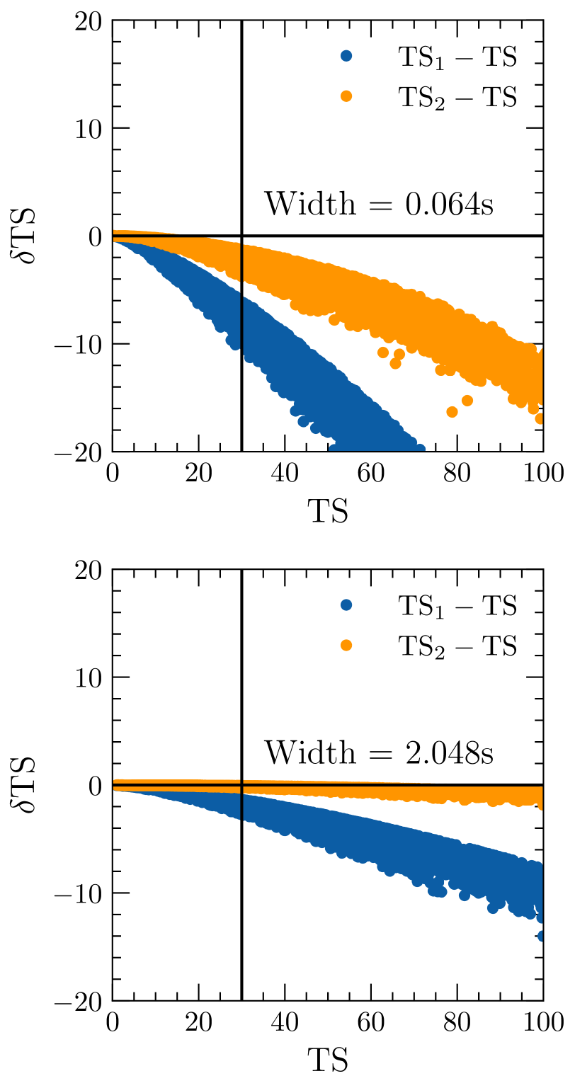
Figure 3: A comparison of exact vs. approximate evaluation of the test statistic for two characteristic time windows. Both estimators agree well for the longer window—which has more photons—while only TS₂ is a sufficient approximation for short search windows.

It is clear (Figure 2) that the approximate estimators TS₁ and TS₂ undershoot the exact $\mathrm{TS_{e}}$. For the purposes of detection, the TS estimator needs only be accurate up to a typical threshold of $\sim$30. To gauge the differences more accurately, we simulate bursts with a small, real signal, in order to shift the distribution to higher values of TS. The results for $\delta t=64$ ms and 2048 ms are shown in Figure 3. Both approximate and exact methods work for the longer window, but in the shorter window, where there are fewer photons, the linear approximation TS₁ is lower than the exact value by up to 30%. In this case, one must either use the better approximation $\mathrm{TS}_{2}$ or use the faster TS₁ but with lower thresholds for narrower time windows.

In summary, the approximate TS estimators work well for detection. To facilitate comparison of results, we henceforth use the TS₂ statistic. Thus, from the simulations yielding Figure 2, we can easily estimate trigger thresholds with a known false positive rate. Given the 10⁷ simulations, we choose a chance false probability of 10^-6, corresponding to a value of TS${}_{2}=29.6$ and $\sigma_{2}=4.7$ and a false positive rate of about 1 per day assuming a minimum $\delta t$ of 64 ms. In general, these trigger thresholds could be sharpened somewhat with operational constraints, e.g. discarding the TS from pixels where the sky is occulted by the earth. We also note that these simulations yield a trigger threshold very close to the on-board GBM trigger ($\sigma_{2}=4.8$).

Finally, we note here that these simulations demonstrate the capability of the algorithm to test the null hypothesis, i.e. if the data consistent with a slowly-varying background. It will in general then detect a wide variety of transient signals, including both pulses of charged particles and bona fide GRBs. Classifying the sources of transients is a post-detection step, which is not the focus of this work. However, in §4 and §5, we show that the TS itself can be used for preliminary classification.

3.3 Transient Sensitivity

We can now determine the detection threshold by simulating many realizations of the alternative hypothesis over a range of fluxes to estimate the fraction yielding a value of TS₂ ($\sigma_{2}$) above the trigger threshold. We adopt two windows, $\delta t=$64 ms and 1024 ms, which are of interest for detection of short GRBs and which facilitate comparison with the catalog of GBM GRBs (von Kienlin et al., 2020).

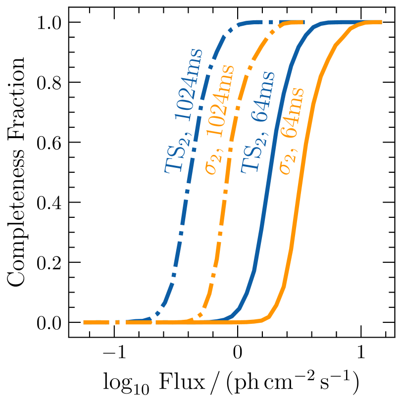
Figure 4: The fraction of simulated bursts producing a test statistic that surpasses the thresholds discussed in the main text, for two time windows, as a function of the 50–300 keV flux of the simulated burst.

The results of these simulations are shown in Figure 4. If we take 50% completeness for a detection threshold, we find values for 64ms of 1.8 ph cm^-2 s^-1 for TS₂ and 3.3 ph cm^-2 s^-1 for $\sigma_{2}$. At 1024 ms, the thresholds are 0.42 and 0.83 ph cm^-2 s^-1, respectively. In summary, the ML algorithm is almost twice as sensitive as the rate-based trigger.

Using the GBM catalog, an instrumental threshold can be estimated from an observed turnover in the 64-ms GRB fluxes at $\sim$3 ph cm^-2 s^-1, in good agreement with our estimate of the $\sigma_{2}$ threshold. However, we note that the real instrument samples a much wider range of background rates and, while its sensitivity peaks in the equatorial plane (instrumental coordinates), this plane generally intersects the earth because the rocking profile exposes less sensitive aspects of the instrument to the sky. We have not attempted to capture such details. Further, these simple simulations assume a top- hat shape burst that is perfectly aligned with the time window used to extract data, and so in general realistic thresholds will be higher. However, these simplifications are common to both algorithms, so we conclude that the use of ML methods could substantially improve the onboard trigger performance of an instrument like GBM.

3.4 Real-time Localization

The localization power of an instrument like GBM or Glowbug depends on the relative brightness of the transient and how much contrast in count rate between detector elements the instrument design provides. The 482 pixels used for the simulations and for the reference implementation below provide a resolution of about 9^∘, which is adequate for estimating the position of transients near threshold but too coarse for precise localization. Here, we assess the reliability of coarse positions that result from the detection algorithm and that might be used in low-latency alerts. We defer discussion of refined, post-detection localization to §6.

If the templates used for detection exactly match the detected burst spectrum, then the maximum-TS pixel should correspond to the true (simulated) direction up to the limits of statistical precision. However, our design mimics real-world applications, with a mismatch between the true spectrum and the templates, and so the inferred positions will be biased.

We determined the size of the bias by simulating 10,000 bright bursts with a 50–300 keV flux of 10 ph cm^-2 s^-1 and a duration of 1.024 s, producing a typical TS_e of 7000. (NB that for localization, it is critical to use the exact TS.) For each simulation, there are three position estimates, i.e. the pixels that maximize the likelihood for each G20 template. In general, these differ, with only 6.4% of the bursts yielding the same coarse position for all three templates. However, by using the pixel/template combination that maximizes the total TS, we recovered the correct position 97% of the time. Of the remaining 3% of bursts with incorrect positions (a substantial systematic error of $\geq$$9^{\circ}$), more than 90% were from bursts simulated with the template that is mid-way between the normal and the hard G20 templatete. From Figure 1, it is apparent that the “distance” between these templates is larger than between the normal and soft templates.

Thus, it is clear that the problem of localization cannot be separated from the question of the true spectrum, and using the wrong template can generate tremendous ($>$10^∘) errors. On the other hand, even with just three templates, the coarse positions from the detection algorithm are correct almost all the time, suggesting the prescription can be used “out of the box” for GRB direction finding and for seeding of follow-up localization.

Near-threshold GRBs will in general be poorly localized, but it is also of interest if the real-time localization of such faint GRBs is also accurate. Using the same approach, but adjusting the source rate to produce a mean TS of about 40, we determined the distribution of the TS difference between the TS-maximizing pixel and the pixel of the true position. We found that $\delta\mathrm{TS}<5.99$ about 92% of the time, in reasonable agreement with the expectation of 95%. Thus, probability maps for faint-GRB localization should be reliable.

4 Reference Implementation

Here, we present a reference implementation (RI) of the ML approach presented in §2 and whose idealized scientific performance was estimated in §3. The RI is designed to work as a real-time transient detection algorithm on $\gamma$-ray sensors and to allow real-world computational and scientific performance evaluations. Parameters governing some aspects of the RI are listed in Table 2; they are fully customizable, but the specific values used in benchmarking are listed.

The base implementation is in C, and a parallel implementation in Python allows rapid prototyping and testing of features. The C implementation—with additional instrument-specific data handling, command and control, and housekeeping layers—also provides the burst detection algorithm for the Glowbug flight software.

Name	Symbol	Description	RI Value
Detector elements	$\mathrm{N_{det}}$	Number of independent detectors	12
Energy channels	$\mathrm{N_{chan}}$	Number of energy channels	8
Transient spectra	$\mathrm{N_{tmpl}}$	Number of spectral templates used for search	3
Incident directions	$\mathrm{N_{pix}}$	Number of spatial pixels/directions to search	482
Input timescale	$\mathrm{\tau_{min}}$	Update timescale for detection algorithm	32 ms
Number of timescales	$\mathrm{N_{F}}$	Hierarchical streams	7 (64 ms–4096 ms)
Background timescale	$\mathrm{\tau_{b}}$	Update timescale for background model	1.024 ms ($32\times\mathrm{\tau_{min}}$)
Background samples	$\mathrm{N_{b}}$	Number of samples used to estimate background	120 / 60 / 30

Table 2: Parameters, all of which are adjustable, used in the reference implementation (RI) of the algorithm. The particular values used in the RI are given in the rightmost column.

4.1 Data Synchronization and Aggregation

For the RI, we abstract away the frontend electronics and assume as input a stream of individual events comprising a detector element index, an energy channel index, and an absolute timestamp. For our RI with 12 detectors, these take the form of a 4-byte word that provides a 1-ms resolution timestamp and an 8-channel energy resolution. We further assume that pseudo-events triggered by clock pulses (PPS, or pulse-per-second) are provided in the datastream from the onboard clock.

We make no assumptions about raw data ordering, so the first step is to synchronize the data over detector elements and bin it into uniform time bins. Data are discarded until the first PPS is received, which determines the epochs. Data are stored in a circular buffer with resolution $\mathrm{\tau_{min}}$ (32 ms), so a bitshift efficiently converts epoch-subtracted timestamps into buffer indices. Data are synchronized by tracking the detector whose last delivered event is the oldest, $t_{\mathrm{synch},n}$. When that detector next delivers data, a new oldest detector is identified, whose latest event is $t_{\mathrm{synch},n+1}$. By construction, all detectors have delivered at least one event after $t_{\mathrm{synch},n+1}$, so all bins with $t_{\mathrm{synch},n}<=t<t_{\mathrm{synch},n+1}$ are synchronized and the buffer indicates these samples are available to downstream processing. The output of this procedure is a uniform time series of counts spectra similar to the CTIME data product of GBM.

It is necessary to consider transients with a wide range of durations, and we adopt the same procedure used onboard GBM, aggregating the data into hierarchical streams that differ in time resolution by 2$\times$. Each stream has two phases. Thus, when each new $\mathrm{\tau_{min}}$ (32-ms) sample arrives, it is combined with the preceding $\mathrm{\tau_{min}}$ sample to update one phase of the $2\mathrm{\tau_{min}}$ (64-ms) resolution stream. It is combined with the next $\mathrm{\tau_{min}}$ sample to arrive to update the second phase. These two phases feed a $4\mathrm{\tau_{min}}$ stream, which updates every $2\mathrm{\tau_{min}}$, etc. The efficient aggregation means that the longest timescales searched for transients are set not by computational constraint but by movement of the spacecraft and by confusion with the time-variable background.

The RI is tickless: whenever new events arrive, they are written into the synchronizing buffer, which will produce 0, 1, or more synchronized, $\mathrm{\tau_{min}}$ samples depending on the specifics of the detector readout scheme. As soon as any samples are available, they are fed into the hierarchical summing and the transient search is run on any updated phases. (So in the RI, the 64 ms-timescale search runs every 32 ms, etc.) Tasks with an inherent timescale are tied to particular streams. E.g., the background mode updates every $\tau_{b}=1.024$ s by tapping one phase of the 1.024 s stream.

We use a 32-bit floating point format for all data, including counts, in the RI. Doing so simplifies data structures, and the memory requirements for the buffer are quite modest, $<$1 MiB per minute of data.

Finally, we briefly consider the computational requirements for the synchronizing buffer, which is the only component of the RI which depends directly on the event rate. In general, operations will depend on the specific data format. In the RI, there are about 10 bitwise operations used to extract and test portions of the 4-byte word, and three integer arithmetic operations (including a modulo) to determine the buffer index to increment. For a typical scintillator, the maximum event rate is set by deadtime and is likely to be $<$$10^{5}$ Hz. For ten such detector elements operating at the maximum rate—an extraordinary circumstance—processing the event data will require $10^{7}$ s^-1 integer operations. This rate is less than the $\approx$2$\times 10^{7}$ floating point operations required for transient searches (§4.3 and §4.6).

Memory
Name	Complexity	Reference	MiB
Synchronizing buffer	$\mathrm{N_{chan}}\mathrm{N_{det}}\times\frac{\mathrm{t_{buff}}}{\mathrm{\tau_{min}}}$	$12\times 8\times\frac{600\,\mathrm{s}}{32\,\mathrm{ms}}$	6.90
Templates	$\mathrm{N_{tmpl}}\mathrm{N_{pix}}\mathrm{N_{chan}}\mathrm{N_{det}}$	$3\times 482\times 8\times 12$	0.53
Floating Point Ops
Name	Complexity	Reference	106 OP s-1
TS1, $+$	$\mathcal{L}_{\mathrm{N_{F}}}\mathrm{N_{tmpl}}\mathrm{N_{pix}}(\mathrm{N_{chan}}\mathrm{N_{det}}+1)/\mathrm{\tau_{min}})$	$3.97\times 3\times 482\times 8\times 12/32\,\mathrm{ms}$	17.4
TS1, $\times$	$\mathcal{L}_{\mathrm{N_{F}}}\mathrm{N_{tmpl}}\mathrm{N_{pix}}(\mathrm{N_{chan}}\mathrm{N_{det}}+1)/\mathrm{\tau_{min}}$	$3.97\times 3\times 482\times 8\times 12/32\,\mathrm{ms}$	17.4
TS1, $\div$	$\mathcal{L}_{\mathrm{N_{F}}}\mathrm{N_{tmpl}}\mathrm{N_{pix}}/\mathrm{\tau_{min}}$	$3.97\times 3\times 482/32\,\mathrm{ms}$	0.18
Bkg. update, $\times$	$\mathrm{N_{tmpl}}\mathrm{N_{pix}}\mathrm{N_{chan}}\mathrm{N_{det}}/\mathrm{\tau_{b}}$	$3\times 482\times 8\times 12/1024\,\mathrm{ms}$	0.14

Table 3: Computational requirements in terms of memory and floating point operations. The second column indicates the theoretical complexity and, where applicable, the memory layout of arrays. The third column gives the specific values for the reference implementation, and the fourth either the required storage in bytes (all storage and operations are implemented with 32-bit precision floating point) or the required number of floating point operations.

4.2 Background Estimation

In §3 we assumed perfect knowledge of the background, but in application it must be estimated. The primary challenge is the orbital variation in both the incident particle background and internal background from activation, especially from passages through the South Atlantic Anomaly (SAA), a region with a high flux of energetic particles. The variations further depend on the orbital precession phase, the solar cycle, and solar flaring activity.

Ideally, background variations could be predicted with parametric models (Biltzinger et al., 2020) or from archival data from earlier orbits. However, with high background count rates, even small errors in the background model produce spurious or missed transient detections. Thus, for the RI we estimate the background with a simple, robust moving average.

Specifically, we collect $\mathrm{N_{b}}$ (120) samples of data from the $\tau_{\mathrm{b}}$ stream (1.024 s) and from this estimate the mean and slope of the count rate for each detector and channel. To avoid overlap of the background samples with those being searched for transients, we project the background estimate forward in time, typically about 4 s.

This linear model can only capture some of the true background variations, so we also attempt to determine if the estimate is consistent with the data. Of particular concern are (1) intervals when the instrument is entering or exiting the SAA, where the background rate may change nonlinearly over the time $\mathrm{N_{b}}\mathrm{\tau_{b}}$, and (2) rapid “spikes” in background due to incident particles, e.g. particle precipitation events. To mitigate the first issue, we invalidate the background estimate if the magnitude of the observed slope exceeds a maximum per-channel value. To mitigate spikes, we observe the residuals of the samples in the background window. If the model is adequate, then these residuals should follow an approximately normal distribution with variance equal to the typical count rate. We test for normality using a kurtosis-only version of the D’Agostino test (D’Agostino & Belanger, 1990), and if there is substantial unmodeled rate variation (exceeding the D’Agostino test threshold), the background model is invalidated.

It is often too restrictive to require linear background variation over $\mathrm{N_{b}}\mathrm{\tau_{b}}=123$ s, so the RI additionally implements nested models operating on $\mathrm{N_{b}}/2$ and $\mathrm{N_{b}}/4$ samples. If the longest window is invalid, the shorter windows are considered, with larger thresholds for the time derivative and D’Agostino test. Whenever the background model is in steady state, the preferred, longest window is used. If a (short) rate excursion occurs, all three windows will fail the check, but within $\mathrm{N_{b}}/4$ samples, the spike will leave the shortest window, which will furnish a new background estimate. $\mathrm{N_{b}}/4$ samples later, the next longest window ($\mathrm{N_{b}}/2$) will be adopted, and finally the spike will exit the full window and steady state is restored. This approach preserves 75% of the exposure compared to a single background window.

In general, most parameters in the RI are adjustable but have been tuned for the orbit and altitude of GBM. We show examples of the background estimator in operation in §5. We expect that this approach will also be suitable for orbits of instruments such as Glowbug (inclination 52^∘) with suitable parameter updates, but may require additional features to capture and mitigate background variations in the auroral zones.

Because the computation associated with the background model update has complexity $\mathcal{O}(\mathrm{N_{det}}\mathrm{N_{chan}})$, it is negligible compared to the evaluation of TS.

4.3 TS Computation

Whenever a new sample becomes available in one of the time-averaged streams, we search for a transient by evaluating TS in a four-dimensional loop over $\mathrm{N_{tmpl}}$ templates (index $k$), $\mathrm{N_{pix}}$ spatial directions ($l$), $\mathrm{N_{chan}}$ energy channels ($i$), and $\mathrm{N_{det}}$ detector elements ($j$). From Equations 10 and 11, the innermost loops are an evaluation of an inner product between the observed counts and the predicted signal-to-background ratio:

$$NT_{kl}= \sum_{i=1}^{\mathrm{N_{chan}}}\sum_{j=1}^{\mathrm{N_{det}}}c_{ij}F_{klij}/b_{ij}\equiv c_{ij}t_{klij}$$ (13)

$$NT^{2}_{kl}= \sum_{i=1}^{\mathrm{N_{chan}}}\sum_{j=1}^{\mathrm{N_{det}}}(c_{ij}t_{klij})t_{klij}$$ (14)

$$NT^{3}_{kl}= \sum_{i=1}^{\mathrm{N_{chan}}}\sum_{j=1}^{\mathrm{N_{det}}}(c_{ij}t^{2}_{klij})t_{klij}.$$ (15)

In the innermost loop, each moment requires a single multiply and add, and so from Equation 10 it is apparent that evaluating TS₁ thus requires $2\mathrm{N_{tmpl}}\mathrm{N_{pix}}(\mathrm{N_{chan}}\mathrm{N_{det}}+1)$ adds and multiplies and $\mathrm{N_{tmpl}}\mathrm{N_{pix}}$ divisions. From Equation 11, evaluating TS₂ requires an additional $\mathrm{N_{tmpl}}\mathrm{N_{pix}}(\mathrm{N_{chan}}\mathrm{N_{det}}+1)$ adds and $\mathrm{N_{tmpl}}\mathrm{N_{pix}}(\mathrm{N_{chan}}\mathrm{N_{det}}+3)$ multiplies. Some architectures are likely to support the sequential multiplies, adds, and assignments via fused operators. Up to negligible factors, TS₂ requires about 50% more multiplies and adds than TS₁. In the RI, the maximum TS for each template is recorded, requiring $\mathrm{N_{tmpl}}\mathrm{N_{pix}}$ floating point comparisons, likely also to be negligible except on hardware where comparisons and jumps are anomalously slow.

It is convenient to scale these computational requirements per input sample. In the RI there are 7 streams (64 ms, 128 ms, …, 4096 ms), so the amortized computations per input are $\mathcal{L}_{N_{F}}\equiv\sum_{i=1}^{\mathrm{N_{F}}}2^{1-i}\approx 1.98\times$ those required to evaluate 64 ms stream. Thus, for evaluation of TS₁, for each $\mathrm{\tau_{min}}$ (32 ms) input sample, there are (amortized) $3.97\mathrm{N_{tmpl}}\mathrm{N_{pix}}(\mathrm{N_{chan}}\mathrm{N_{det}}+1)$ adds and multiplies, $3.97\mathrm{N_{tmpl}}\mathrm{N_{pix}}$ divides, and $\mathrm{N_{tmpl}}\mathrm{N_{pix}}\mathrm{N_{chan}}\mathrm{N_{det}}\mathrm{\tau_{min}}/\mathrm{\tau_{b}}$ multiplies for the background update.

The most substantial ancillary computation is the pre-computation of $t_{klij}$, requiring $\mathrm{N_{tmpl}}\mathrm{N_{pix}}\mathrm{N_{chan}}\mathrm{N_{det}}$ multiplies every $\tau_{b}$ s. When the background model is “bad”, $t$ is set to 0, producing 0 for all evaluations of TS.

In addition to the standard, template-based TS computation, we have determined that a per-channel TS can help to identify transients due to spikes in the particle background. The most useful of these are the lowest channel, appropriate for soft electrons, and the highest channel, typically for rapidly rising proton rates on entering the SAA. The per-channel TS computation is very similar to that outlined above, but requires additional overhead in the “channel” loop that is surprisingly expensive. In the RI, we compute the per-channel TS for all $\mathrm{N_{chan}}$ channels, but suggest it should be tuned to application. We have further chosen a memory layout that simplifies programming logic (there is always a sum over $\mathrm{N_{det}}$ in the innermost loop), but swapping the innermost two dimensions may be favorable on some architectures.

4.4 Triggering

In general, any TS value—from any stream—that surpasses a pre-defined threshold value could be considered a trigger. However, it may be advantageous to prefer longer time windows, which generally improve statistical precision, have reduced trials factors, and could provide better seed localizations for follow-up analysis. Further, the use of per-channel TS can help to reject background variations, and we have found that this is more effective with the improved precision of longer time windows.

Thus we distinguish a local trigger—any time the TS surpasses the threshold value—from a global trigger, which is evaluated only on the longest averaging timescale and which can change the instrument mode to a triggered state.

Name	Processor	Clock Speed	GFLOPs
Xeon	Intel Xeon W-2123	3.6 GHz	13.0
Rpi4	ARM Cortex A72	1.5 GHz	1.7
Q8	ARM Cortex A53	1.2 GHz	0.5

Table 4: Brief specifications for benchmark systems.

	Xeon	Xeon	RPi4	RPi4	Q8	Q8
Task	Time (s)	Fractional	Time (s)	Fractional	Time (s)	Fractional
Event processing	0.26	$4.8\times 10^{-5}$	0.54	$1.0\times 10^{-4}$	–	–
Bkg model and update	0.29	$5.4\times 10^{-5}$	0.99	$1.8\times 10^{-4}$	–	–
TS1	9.36	$1.7\times 10^{-3}$	61.11	$1.1\times 10^{-2}$	148	$2.7\times 10^{-2}$
TS2	11.92	$2.2\times 10^{-3}$	85.35	$1.6\times 10^{-2}$	183	$3.5\times 10^{-2}$
Per-channel TS1	15.34	$2.8\times 10^{-3}$	38.54	$7.1\times 10^{-3}$	98	$1.8\times 10^{-2}$
Per-channel TS2	17.41	$3.2\times 10^{-3}$	56.56	$1.0\times 10^{-2}$	115	$2.1\times 10^{-2}$
Other	$<$0.30	$5.6\times 10^{-5}$	$<$1.48	$2.7\times 10^{-4}$	–	–
Total	29.99	$5.6\times 10^{-3}$	145.52	$2.7\times 10^{-2}$	298	$5.5\times 10^{-2}$

Table 5: Execution times required to process 5400 s of data. The “Time” columns indicate the absolute processing time, while the “Fractional” columns give the ratio of the processing time to the total time (5400 s). In all cases, the TS computation dominates the run time, and in all cases, the total fractional processing time is $\ll$1, indicating suitability for real-time operation. Note that TS₂ times are inclusive of the time required to compute TS₁.

We assess the presence of a global trigger as follows. For each update of the longest timescale (4096 ms, every 2048 ms), we check for local triggers in all of the shorter windows that overlap the global window and select the one with the highest TS. E.g. in the event of a very short GRB (say 160 ms), then the 128 ms window should be selected, while a long GRB (say 20 s) should produce the highest TS in the 4096 ms window.

We select the optimal window for both the template TS and for the per-channel TS from the lowest- and highest-energy channels. If these per-channel TS values are comparable or greater than the template TS, it indicates the transient consists primarily of very soft or very hard particles and is thus likely associated with charged particle background. In the RI, a global trigger is initiated when the template TS exceeds both the soft and hard-channel TS by a factor of 1.3.

4.5 GBM Data Playback

We use GBM data both for the benchmarks reported below and in §5 to test the scientific performance of the transient search algorithm. To do this, we break the archival data set up into 1-day intervals, and further divide this data set into “orbits”, which are determined either when GBM enters the SAA or when 90 minutes have elapsed.

For each day, we begin with the archival TTE format data and take the intersection of the Good Time Intervals for each detector. We re-channelize the data from the original 256 to approximately match the 8 desired channel boundaries. We insert PPS events into the data stream at each 1-s boundary, then group data into packets of up to 250 events, converting each event timestamp, channel, and PPS flag into the 4-word format used by the RI (and by Glowbug). Finally, we order the packets according to the timestamp of the last event in them, thus emulating the staggered data delivery expected in real-time application.

4.6 Benchmarking

To compare with the floating point complexity estimates made above, and to provide realistic performance expectations, we benchmark the RI on several distinct platforms. Specifically, we play back the first 5400 s of GBM data acquired on 9 Feb 2014, which has an average summed event rate (within the energy range) of 7.3 kHz. For each platform, we consider the following scenarios:

• The RI is run with the TS computation disabled. This allows estimation of overhead and the event processing rate, further isolated with the use of gprof.

• The RI with template-based TS₁ computation enabled.

• The RI with template-based TS₂ computation enabled.

• The RI with template and channel-based TS₁ computation enabled.

• The RI with template and channel-based TS₂ computation enabled.

Together, these benchmarks provide a full indication of the computational requirements for real-time use on an arbitrary platform.

For each hardware platform, we adopt the compiler command gcc -pg -g -O3 -ftree-vectorize -ffast-math -march=native -std=c11. Further, we use the “linpack” benchmark to estimate a characteristic single-precision, single-threaded floating point performance (Table 4).

There are exactly 168718 32 ms samples processed in the benchmark run, and so from Table 3, we expect the TS₁ calculation to require, in the inner loop, $9.3\times 10^{10}$ each of adds and floats. For the Xeon, with estimated single-precision floating point rate of 13 GFLOPs, the estimated required time is 14.3 s, about 50% higher than the observed value, indicating some effectiveness of SIMD vectorization of loops. We expect that an implementation with hard-coded loop invariants ($\mathrm{N_{det}}$, $\mathrm{N_{chan}}$, etc. could all be fixed in a flight system) would produce more aggressively optimized code, as would manual implementation of the inner loop assembly code. However, the code is already very fast on a Xeon, requiring $<$1% processor utilization on a single core to process the data in real-time equivalent.

The Cortex A72 on the Raspberry Pi 4 is a much less performant processor, running at half the clock speed and with much smaller pools of cache and functional units. As it is also the flight processor for Glowbug, the performance on this platform is critical. It completes the benchmark run about 5$\times$ slower than the Xeon, meaning it is capable of real-time data processing with $<$3% processor utilization.

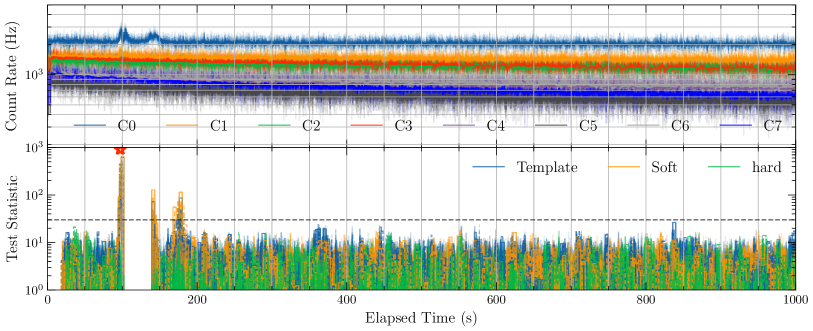
Figure 5: Example of the application of the maximum likelihood algorithm to archival GBM data from 08 Feb 2014 beginning at MET 413575773.952. The top panel shows the count rate summed over all 12 NaI detectors and grouped into the 8 energy channels listed in Table 1. The rate decreases as energy increases. All streams are shown overlaid, with the faster ones using a higher degree of transparency. The top panel gives the maximum template TS (over 482 positions and the three G20 templates) Also shown are the soft-channel and hard-channel TS values. There is a clear transient, generated by incident electrons, which appears primarily in the soft channel C0, though the initial pulse is also visible in channel C1 ($>$50 keV). These particles generate a local trigger (unfilled red star), but because the soft-channel TS is comparable to the template TS, no global trigger is issued. The transient causes the background model to be flagged as invalid while the initial pulse lies in the background window; during these intervals, TS$=$0. The remainder of the 1 ks of data show a steady count rate and correspondingly a TS well below threshold (indicated here by the black dashed line at TS$=$30).

Finally, we consider a processor designed specifically for space applications, the radiation-hardened Xiphos Q8. Its system-on-a-chip includes a 4-core Cortex A53 as well as an FPGA fabric, though we consider only evaluation of the CPU. We built a custom yocto image with czmq support and cross-compiled the RI. Evaluation of the full suite at real-time requires $<$6% utilization of a single core, and the scaling is in good agreement with the relative difference in floating point performance compared to the A72.

In summary, the RI implementation supports real-time ML-based burst detection on processors likely to be selected for a deployment in space, both at low- and high-cost levels.

5 Real-world Detection Performance

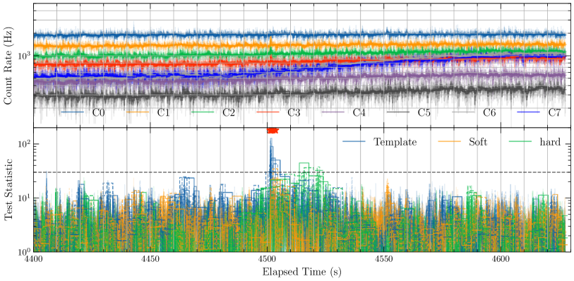
Figure 6: As Figure 5, but showing data beignning at MET 524661967.952, a few minutes surrounding GRB 170817A. The GRB is clearly detected and generates a global trigger (filled red star). The maximum observed TS is 107, occurring in the 256 ms streams. Since the GRB is relatively faint, the background model remains valid.

Here we show two examples of applying the RI implementation to archival GBM data. The first, in Figure 5, shows 1000 ks of data containing a pulse of incident electrons on top of an otherwise slow evolution of the background rates. This example illustrates the computation of TS. Several local triggers are generated in the faster streams because the TS is a random variable and suffers more noise in short time windows. On the other hand, in the longer windows, the template TS is always lower than the soft-channel TS. These local triggers are vetoed and indicated by the unfilled red stars. Extensive testing has shown this prescription is an effective means of identifying such particle transients, even excluding soft events to mimic an instrument with a higher threshold (30–50 keV) compared to GBM. (The $\sim$10 keV threshold for GBM makes electron events particularly obvious.) Following the arrival of the first bright electron pulse, the background model begins to fail the self-consistency check and is flagged as invalid, which automatically sets TS to 0. Following the initial pulse, the background model is re-established. The fainter, slower electron pulses only generate large values of TS in the slow streams and are always vetoed.

The second example shows the ML algorithm applied to GRB 170817A. It generates a global trigger (filled star) with a maximum TS₂ of 118 in the 256 ms window. Goldstein et al. (2017) note that the GRB generated significant detections in three detectors, and that the strongest signal was achieved with the 512 ms filter, with the second-highest significance yielding a $\sigma_{2}$ of 6.3$\sigma$. Consequently GBM would have detected GRB 170817A onboard if it were up to 40% fainter. On the other hand, with a reasonable threshold of TS$=30$, the ML approach would have allowed GBM to detect GRB 170817A if it were 4.3$\times$ fainter! Alternatively, it could have detected it at twice the distance, increasing the rate of such GRBs by about 8. This claim is somewhat conservative because the RI only uses data $>$30 keV.

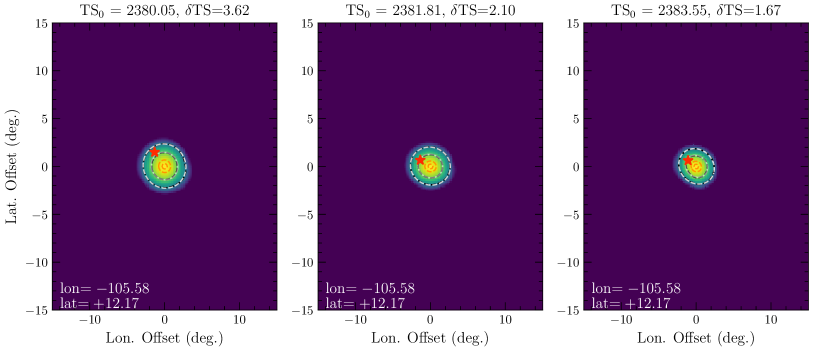
Figure 7: The TS map for three resolutions of the RM, using 192 (left), 642 (center) and 2562 (right) pixels. The TS is evaluated on a 15^∘$\times$15^∘ grid in Cartesian projection around the position that maximizes the overall TS. The true (simulated) position of the transient appears as a red star. The black contours indicate TS drops of 5.99 and 2.30, corresponding to 95% and 68% confidence regions. The red contours indicate TS drops of 0.5 and 0.1, simply for reference. The white contours indicate the 68% and 95% confidence regions for the error ellipse that best fits the TS surface. The simulated transient position is annotated at lower left, and the resulting maximum TS and the TS difference between the simulated position and the best-fit position ($\delta$Ts) are annotated above each panel.

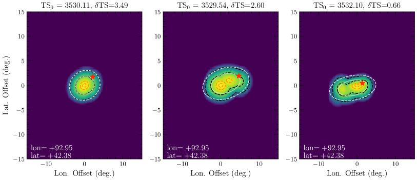
Figure 8: As Figure 7, but showing a case where the higher spatial resolution RM reveals a more complicated TS map.

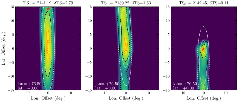
Figure 9: As Figure 7, but for a transient incident from the southern hemisphere, producing elongated and complex uncertainty regions.

6 Precise Localization

As discussed and validated above, ML-based detection automatically provides coarse localizations. In principle, finer real-time localizations could be obtained simply by searching over more directions, but degree-scale precision is likely too expensive for low-power processors. Instead, these coarse localizations are appropriate as seeds for a follow-up analysis that produces a refined position estimate.

The RI does not have such a follow-up capability, but the additional computational complexity is small. A straightforward approach is to generate a degree-scale “TS map” by evaluating the TS over a grid that covers the full coarse pixel from the seed location. Such a map is sufficient to generate a centroid and confidence region and requires only $\sim$100 additional TS evaluations, a negligible increase on those performed by the detection algorithm.

Here, we test how well this procedure might work—and the reliability of ML localizations generally. It is well-demonstrated that GBM localizations—which use ML—suffer from a systematic error of a few degrees (Connaughton et al., 2015). Such localizations rely on two key ingredients: the “true” spectrum of the burst, and the “true” instrument RM to that burst. The GBM RM is based on Monte Carlo particle transport simulations (Kippen et al., 2007; Hoover et al., 2008) of the Fermi Gamma-ray Space Telescope sampled over 272 incident directions. If the mass model used in the simulations is incomplete or inaccurate, then the RM will also suffer inaccuracies. On the other hand, Berlato et al. (2019) note the importance of an accurate spectral template and claim to reduce systematic errors by using using more degrees of freedom in the spectral model.

We consider a related possibility: the effect of the number of pixels used in the representation of the RM. To do this, we used SWORD (Duvall et al., 2019) to create a detailed mass model for Glowbug (instrument only), performed Monte Carlo simulations of an incident broadband $\gamma$-ray spectrum on Glowbug with the underlying GEANT4 (Allison et al., 2016) radiation transport package, and evaluated the RM at three spatial resolutions, using 192, 642, and 2562 incident directions. We do not consider atmospheric scattering, which is an important consideration in GRB localization but which essentially only changes the response matrix.

We then simulated 2000 realizations of data as in §3 with the following differences: (1) we used the 2562-pixel Glowbug RM instead of the GBM RM; (2) we used only the “normal” G20 template (but continue to select a random incident pixel) with a 50–300 keV flux of 3 ph cm^-2 s^-1; (3) we simulated 1.024 s time windows; (4) we restricted the incidence polar angle to $\cos\theta>0$, i.e. the portions of the sky with the best Glowbug sensitivity. These parameters yield a fairly bright burst relative to the background that can typically be localized with a precision of a few degrees. For each simulation, we processed the data using the three spatial resolutions, specifically (1) determining the coarse pixel that maximized the TS according to the GRB template; (2) adaptively refining the localization by spherically, linearly interpolating the instrument response to predict the counts on a finer grid; and (3) producing a final 15^∘$\times$15^∘ TS map on a uniform (Cartesian projection) grid around the maximum TS position. NB that unlike as in §3, we use the same GRB spectral template for both simulation and evaluating the TS in order to isolate the systematic effect of RM resolution.

A good localization must deliver accurate estimates of both the position and its uncertainty, since the latter often governs whether or not it is possible to follow-up transients with narrow-field instruments. The TS is a random field distributed as $\chi^{2}_{2}$, so confidence intervals around the best-fit position can be estimated as, e.g., the contour by which the TS drops from the maximum value by 2.30 (68%) or 5.99 (95%). Alternatively, for cases where the likelihood surface is not particularly gaussian, the likelihood can be combined with a uniform prior and treated numerically to derive Bayesian credible intervals. Thus, we can assess the quality of the localization by analysis of the TS maps produced for the three resolution levels.

The TS maps from the simulations can be grouped into several classes. An example from most common class appears in Figure 7. The transient is well-localized at all three resolutions, and the uncertainty contours are effectively gaussian, as indicated by the agreement between the TS map contours with a quadratic fit to the surface. Such a result could be accurately encapsulated as a single position and an uncertainty ellipse. As the spatial resolution of the RM increases, the size of the error ellipse decreases. (The TS difference between the simulated position and the best-fit position also decreases.) As we will see, this is a general trend.

The second example, Figure 8, shows a class where the smoothing in the low-pixel RM generates misleadingly gaussian TS maps while the high-pixel RM yields a TS map with a more complicated structure. In these cases, it is more suitable to describe the position with the full map. This more complex surface includes the true position in the high-probability region, whereas it is in low-probability region (outside the 95% contours) in the low-resolution versions.

Finally, we consider a transient incident in the equatorial plane of Glowbug. Because the detectors form a half cube, such low-latitude bursts can be moved “up” and “down” without changing the predicted counts very much, and the uncertainty regions thus become narrow ellipses, as shown in Figure 9. Here, because the true count rate varies little over the long ellipse, the systematic differences between the RMs are magnified, and we see the high-resolution RM yields a TS map with substantially more structure and that again better includes the true position.

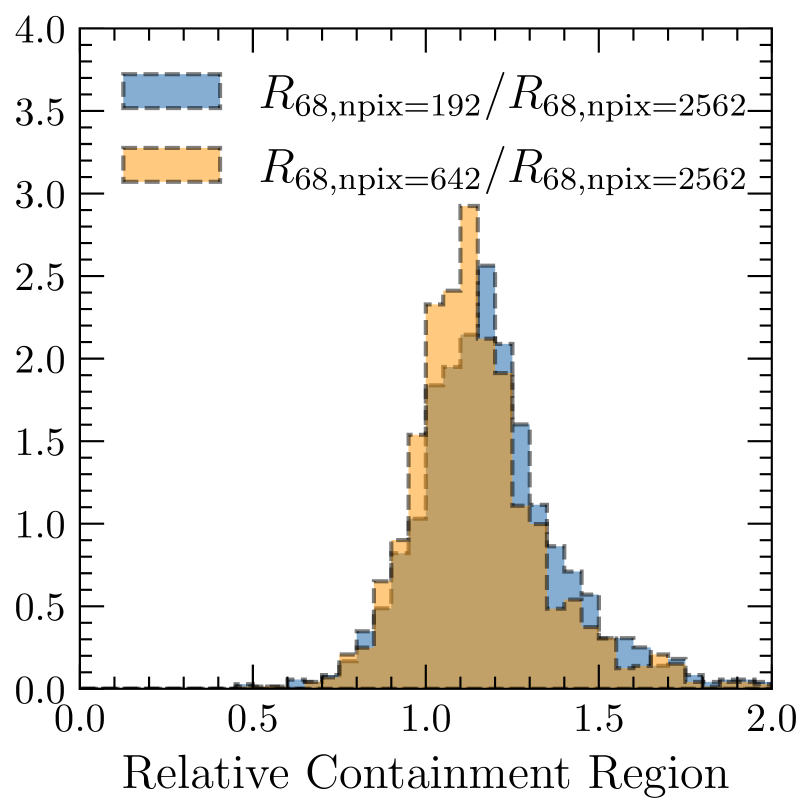
Figure 10: The distribution of relative sizes of the size of the 68% confidence region, $R_{68}$, for the two low-resolution RMs as compared to the highest-resolution version.

Figure 11: The cumulative distribution of the offset in position between the simulated and best-fit position, scaled by the size of the uncertainty region. Specifically, this is estimated from the cumulative $\chi^{2}_{2}$ distribution evaluated for the difference in TS between the positions. If the positions and uncertainty regions are accurate, the distribution should be linear.

To synthesize these results, we consider two key questions: what is the relative size of the uncertainty regions, and how often is the true position of the transient within them? In Figure 10, we show the relative ratios of sizes of $R_{68}$, the region expected to contain the true transient position 68% of the time, estimated directly from the TS map as the summed area of all pixels within $\delta\mathrm{TS}<2.30$ of the peak. From this, it is clear that the confidence regions are larger when using the low-resolution RMs: the median region is 17% larger for 192 pixels and 13% for 642 pixels. But the tails are heavy, with e.g. 16% of the regions are 40% larger (192 pixels) and 33% larger; and the worst 5% of the regions are 61% larger and 54% larger, respectively.

Next, we consider the reliability of the uncertainty regions, which is best assessed by considering the difference in TS between the best-fit and simulated positions, $\delta$TS. The probability to observe a transient with a given offset is then simply $p=\int_{0}^{\delta\mathrm{TS}}\chi^{2}_{2}(x)\,dx$. Then, if the TS distribution truly follows the $\chi^{2}_{2}$ distribution (the uncertainty estimates are accurate), $p$ should follow a uniform distribution. Figure 11 shows the cumulative distribution of $p$, from which it is clear that the low-pixel RMs yield likelihood surfaces that underestimate the uncertainty, particularly for the 192-pixel version.

All of these effects would be magnified if considering even more off-axis bursts with $\cos\theta<0$. In conclusion, we find that it is critical to use a high-resolution response matrix, with about an order of magnitude more pixels than are currently in use by, e.g., GBM analysis tools. Doing so yields both improved constraints on position and reduces systematic error stemming from inaccuracies in the TS maps used to infer positions. The magnitude of these errors are often several degrees, in the case of these bright bursts, and thus it is plausible that this imprecision in the RM, along with potential inaccuracies in the Fermi mass model, contributes substantially to the observed systematic errors in GBM positions.

7 Discussion

We have developed maximum likelihood algorithms that are fast enough to run in real-time on low-power processors. Their trigger thresholds can be calibrated with a predictable false-positive rate, and for a given trigger threshold they deliver a detection threshold about half that of existing on-board triggers. In a test with archival GBM data (GRB 170817A), the sensitivity was improved by more than $4\times$.

From an instrumental design standpoint, this is a substantial sensitivity boost. With thin scintillators, both the signal and background rates scale approximately linearly with effective area, $A$, so the signal-to-noise ratio for a given transient only scales as $\sqrt{A}$. Because we have shown that the computational burden is modest and requires no unusual hardware, adopting ML algorithms allows an instrument to reach the same sensitivity as one about four times larger for “free”.

From a scientific standpoint, it is also a substantial gain. The transients of most interest for multimessenger astronomy are relatively nearby, and thus uniformly distributed through a detection volume such that $\log N$–$\log S\propto S^{-3/2}$. This degree of improvement of sensitivity yields a transient rate that is increased to $1.8^{\frac{3}{2}}$ to $2.0^{\frac{3}{2}}$ (240–280%) of the baseline rate.

We note that with GBM data, this sensitivity improvement can be and has already been exploited in the “sub-threshold” search pipeline (Blackburn et al., 2015; Kocevski et al., 2018), which is possible post facto because GBM can downlink every photon event with TDRSS. (In principle the CTIME data would be sufficient for ML detection, but the low spectral resolution would complicate analysis.) Access to such high-bandwidth telemetry is not guaranteed for future experiments, and in particular Starburst will not be able to send its full event data to the ground. However, we have shown it is possible to realize ML techniques with on-board processing, ensuring that faint transients can be identified while only downlinking data of interest.

Because the RI presented here only requires $<$10% of a single core of low-power processors, we can consider even more ambitious applications. Possibilities include searches for ms-scale transients, such as terrestrial $\gamma$-ray flashes (TGFs, e.g. Roberts et al., 2018) or the use of a truly fine spatial grid to provide real-time near-degree-scale localizations. At a minimum, the use of an expanded library of GRB templates relative to the RI could reduce systematic errors in rapid localization. Such rapid, accurate localization would facilitate robotic follow-up observations of rapidly-fading afterglows.

Our investigation into the robustness of precise burst localization revealed a surprising dependence on the spatial resolution of the instrument RM, and we suspect this effect contributes to the systematic uncertainty of GRB localizations with GBM. Goldstein et al. (2020) find evidence for a two-component model in which about half of GRBs have a small uncertainty concentrated around $\sim$2^∘, and the other half occupy a long tail with a typical value of $\sim$4^∘. (Previous analyses of BATSE data (Briggs et al., 1999) and GBM data (Connaughton et al., 2015) found similar distributions.) Both values are consistent with classes of systematic errors we observed in our analysis with low-resolution RMs, and we speculate that the two components may simply result from the proximity of the true GRB position to one of the RM sampling points. This idea could be tested with a higher-resolution RM for GBM. We used the Glowbug RM for our study because we had developed substantial machinery for creating mass models, performing Monte Carlo, and parsing the results into detector RMs. The GBM mass model is substantially more complicated (including the entire Fermi spacecraft), and creating a higher resolution RM is a substantial undertaking. However, archival and future GBM data are critical for multi-messenger astronomy, and obtaining more reliable localizations make it a worthwhile endeavor.

Finally, the relative ease of performing ML detection on-board also informs GRB experimental design. In particular, it increases the value of instruments with good “geometry factors”, i.e. those that expose discrete detector elements to different portions of the sky, like GBM. Given the rapidly improving availability of affordable SmallSat spacecraft buses and the development of large-area (heavy) scintillator detectors, this medium-scale form factor may be the “sweet spot” for future networks of $\gamma$-ray sensors.

References

- Allison et al. (2016) Allison, J., Amako, K., Apostolakis, J., et al. 2016, Nuclear Instruments and Methods in Physics Research A, 835, 186, doi: 10.1016/j.nima.2016.06.125
- Barthelmy et al. (2005) Barthelmy, S. D., Barbier, L. M., Cummings, J. R., et al. 2005, Space Sci. Rev., 120, 143, doi: 10.1007/s11214-005-5096-3
- Berlato et al. (2019) Berlato, F., Greiner, J., & Burgess, J. M. 2019, ApJ, 873, 60, doi: 10.3847/1538-4357/ab0413
- Biltzinger et al. (2020) Biltzinger, B., Kunzweiler, F., Greiner, J., Toelge, K., & Burgess, J. M. 2020, A&A, 640, A8, doi: 10.1051/0004-6361/201937347
- Blackburn et al. (2015) Blackburn, L., Briggs, M. S., Camp, J., et al. 2015, ApJS, 217, 8, doi: 10.1088/0067-0049/217/1/8
- Briggs et al. (1999) Briggs, M. S., Pendleton, G. N., Kippen, R. M., et al. 1999, ApJS, 122, 503, doi: 10.1086/313221
- Connaughton et al. (2015) Connaughton, V., Briggs, M. S., Goldstein, A., et al. 2015, ApJS, 216, 32, doi: 10.1088/0067-0049/216/2/32
- D’Agostino & Belanger (1990) D’Agostino, R. B., & Belanger, A. 1990, The American Statistician, 44, 316
- Duvall et al. (2019) Duvall, W., Phlips, B., Hutcheson, A., et al. 2019, in 2019 IEEE International Symposium on Technologies for Homeland Security (HST), 1–6
- Frontera & von Ballmoos (2010) Frontera, F., & von Ballmoos, P. 2010, X-Ray Optics and Instrumentation, 2010, 215375, doi: 10.1155/2010/215375
- Goldstein et al. (2017) Goldstein, A., Veres, P., Burns, E., et al. 2017, ApJ, 848, L14, doi: 10.3847/2041-8213/aa8f41
- Goldstein et al. (2020) Goldstein, A., Fletcher, C., Veres, P., et al. 2020, ApJ, 895, 40, doi: 10.3847/1538-4357/ab8bdb
- Hoover et al. (2008) Hoover, A. S., Kippen, R. M., Wallace, M. S., et al. 2008, in American Institute of Physics Conference Series, Vol. 1000, Gamma-ray Bursts 2007, ed. M. Galassi, D. Palmer, & E. Fenimore, 565–568
- Kippen et al. (2007) Kippen, R. M., Hoover, A. S., Wallace, M. S., et al. 2007, in American Institute of Physics Conference Series, Vol. 921, The First GLAST Symposium, ed. S. Ritz, P. Michelson, & C. A. Meegan, 590–591
- Klebesadel et al. (1973) Klebesadel, R. W., Strong, I. B., & Olson, R. A. 1973, ApJ, 182, L85, doi: 10.1086/181225
- Kocevski (2022) Kocevski, D. 2022, Bulletin of the AAS, 54
- Kocevski et al. (2018) Kocevski, D., Burns, E., Goldstein, A., et al. 2018, ApJ, 862, 152, doi: 10.3847/1538-4357/aacb7b
- Kouveliotou et al. (1993) Kouveliotou, C., Meegan, C. A., Fishman, G. J., et al. 1993, ApJ, 413, L101, doi: 10.1086/186969
- Levan et al. (2014) Levan, A. J., Tanvir, N. R., Starling, R. L. C., et al. 2014, ApJ, 781, 13, doi: 10.1088/0004-637X/781/1/13
- McEnery et al. (2019) McEnery, J., van der Horst, A., Dominguez, A., et al. 2019, in Bulletin of the American Astronomical Society, Vol. 51, 245
- Meegan et al. (2009) Meegan, C., Lichti, G., Bhat, P. N., et al. 2009, ApJ, 702, 791, doi: 10.1088/0004-637X/702/1/791
- Meegan et al. (1992) Meegan, C. A., Fishman, G. J., Wilson, R. B., et al. 1992, Nature, 355, 143, doi: 10.1038/355143a0
- Mitchell et al. (2021) Mitchell, L., Phlips, B., Johnson, W. N., et al. 2021, Nuclear Instruments and Methods in Physics Research A, 988, 164798, doi: 10.1016/j.nima.2020.164798
- Poolakkil et al. (2021) Poolakkil, S., Preece, R., Fletcher, C., et al. 2021, ApJ, 913, 60, doi: 10.3847/1538-4357/abf24d
- Roberts et al. (2018) Roberts, O., Fitzpatrick, G., Stanbro, M., et al. 2018, Journal of Geophysical Research: Space Physics, 123, doi: 10.1029/2017JA024837
- Tomsick et al. (2019) Tomsick, J., Zoglauer, A., Sleator, C., et al. 2019, in Bulletin of the American Astronomical Society, Vol. 51, 98
- von Kienlin et al. (2020) von Kienlin, A., Meegan, C. A., Paciesas, W. S., et al. 2020, ApJ, 893, 46, doi: 10.3847/1538-4357/ab7a18
- Wilks (1938) Wilks, S. S. 1938, The Annals of Mathematical Statistics, 9, 60 , doi: 10.1214/aoms/1177732360
- Woolf et al. (2022) Woolf, R. S., Grove, J. E., Briggs, M. S., et al. 2022, in Space Telescopes and Instrumentation 2022: Ultraviolet to Gamma Ray, ed. J.-W. A. den Herder, S. Nikzad, & K. Nakazawa, Vol. 12181, International Society for Optics and Photonics (SPIE), 121811O. https://doi.org/10.1117/12.2630543