Implications for the non-Gaussianity of curvature perturbation
from pulsar timing arrays

Abstract

The recently released data by pulsar timing array (PTA) collaborations present strong evidence for a stochastic signal consistent with a gravitational-wave background. Assuming this signal originates from scalar-induced gravitational waves, we jointly use the PTA data from the NANOGrav 15-yr data set, PPTA DR3, and EPTA DR2 to probe the small-scale non-Gaussianity. We put the first-ever constraint on the non-Gaussianity parameter, finding $|F_{\mathrm{NL}}|\lesssim 13.9$ for a lognormal power spectrum of the curvature perturbations. Furthermore, we obtain $-13.9\lesssim F_{\mathrm{NL}}\lesssim-0.1$ to prevent excessive production of primordial black holes. Moreover, the multi-band observations with the space-borne gravitational-wave detectors, such as LISA/Taiji/TianQin, will provide a complementary investigation of primordial non-Gaussianity. Our findings pave the way to constrain inflation models with PTAs.

Introduction. Various inflation models (see e.g. Armendariz-Picon et al. (1999); Garriga and Mukhanov (1999); Kobayashi et al. (2010); Arkani-Hamed et al. (2004); Alishahiha et al. (2004); Baumann et al. (2016); Seery and Lidsey (2005); Kobayashi et al. (2011)) predict the existence of a sizable primordial non-Gaussianity, making it an important role in exploring the early Universe Baumann and Green (2011, 2012); Kristiano and Yokoyama (2022). How to probe the non-Gaussianity of the Universe is one of the key questions in modern physics. Over several decades, significant advancements have been made in precisely measuring a nearly scale-invariant power spectrum characterizing primordial density fluctuations. These measurements have been accomplished through the utilization of observational data from the cosmic microwave background (CMB) Aghanim et al. (2020a) and large-scale structure Alam et al. (2021); Pandey et al. (2022) surveys, offering valuable insights into the fundamental properties of the Universe. Although significant efforts have been dedicated to precisely characterizing power spectra of primordial perturbations on large scales, searching for new and independent probes becomes crucial when examining phenomena at the small scale.

Gravitational waves (GWs) offer a fascinating avenue for acquiring insights into the history and composition of the Universe, serving as another probe of small-scale non-Gaussianity. In fact, space-borne GW detectors, such as LISA Amaro-Seoane et al. (2017), Taiji Ruan et al. (2020), and TianQin Luo et al. (2016), can explore the non-Gaussianity through scalar-induced GWs (SIGWs) Tomita (1967); Saito and Yokoyama (2009); Young et al. (2014); Cai et al. (2019a, b); Kohri and Terada (2018); Yuan et al. (2019, 2020a); Chen et al. (2020); Yuan et al. (2020b) in the mHz frequency band. Pulsar timing arrays (PTA) Sazhin (1978); Detweiler (1979), on the other hand, are sensitive in the nHz frequency band, providing another opportunity to probe the early Universe. Recently, NANOGrav Agazie et al. (2023a, b), PPTA Zic et al. (2023); Reardon et al. (2023), EPTA+InPTA Antoniadis et al. (2023a, b), and CPTA Xu et al. (2023) all announced the evidence for a stochastic signal in their latest data sets consistent with the Hellings-Downs Hellings and Downs (1983) spatial correlations expected by a stochastic gravitational-wave background (SGWB). Although there can be a lot of sources Li et al. (2019); Vagnozzi (2021); Chen et al. (2021); Wu et al. (2022a); Chen et al. (2022a); Benetti et al. (2022); Chen et al. (2022b); Ashoorioon et al. (2022); Wu et al. (2022b, 2023a); Falxa et al. (2023); Wu et al. (2023b); Dandoy et al. (2023); Madge et al. (2023) in the PTA window, whether this signal is of astrophysical or cosmological origin is still under intensive investigation Afzal et al. (2023); Antoniadis et al. (2023c); King et al. (2023); Niu and Rahat (2023); Datta and Samanta (2023); Vagnozzi (2023); Bi et al. (2023); Wu et al. (2023c); Jin et al. (2023); Liu et al. (2023a); Yi et al. (2023a); Agazie et al. (2023c); Yi et al. (2023b); You et al. (2023); Chen et al. (2023a).

A possible explanation for this signal is the SIGW produced by the primordial curvature perturbations at small scales. When the primordial curvature perturbations reach significant magnitudes, they can generate a considerable SGWB through second-order effects resulting from the non-linear coupling of perturbations. Additionally, large curvature perturbations can trigger the formation of primordial black holes (PBHs) Zel’dovich and Novikov (1967); Hawking (1971); Carr and Hawking (1974). PBHs have attracted a lot of attention in recent years Belotsky et al. (2014); Carr et al. (2016); Garcia-Bellido and Ruiz Morales (2017); Carr et al. (2017); Germani and Prokopec (2017); Chen et al. (2019); Liu et al. (2019a); Chen and Huang (2018); Liu et al. (2019b); Fu et al. (2019); Liu et al. (2020a); Cai et al. (2020); Chen and Huang (2020); Liu et al. (2020b); Fu et al. (2020); De Luca et al. (2021a); Wu (2020); Vaskonen and Veermäe (2021); De Luca et al. (2021b); Domènech and Pi (2022); Hütsi et al. (2021); Chen et al. (2022c); Kawai and Kim (2021); Braglia et al. (2021); Liu et al. (2023b); Braglia et al. (2023); Zheng et al. (2023); Liu et al. (2023c); Meng et al. (2023); Chen et al. (2023b, c); Guo et al. (2023) (see also reviews Sasaki et al. (2018); Carr et al. (2021); Carr and Kuhnel (2020)) as a promising candidate for dark matter and can explain the binary black holes detected by LIGO-Virgo-KAGRA Bird et al. (2016); Sasaki et al. (2016). The formation rate of PBHs would be entirely altered if there is any significant non-Gaussianity, as PBHs are produced at the large amplitude tail of the curvature perturbation probability distribution Young and Byrnes (2013).

In this letter, assuming that the signal detected by PTAs is from SIGWs, we jointly use the NANOGrav 15-yr data set, PPTA DR3, and EPTA DR2 to constrain the small-scale non-Gaussianity when the scalar modes re-enter the horizon. As a demonstration, we employ a lognormal power spectrum of curvature perturbations and constrain the non-Gaussianity parameter as $-13.9\lesssim F_{\mathrm{NL}}\lesssim-0.1$.

SIGWs and PBHs. We will briefly review the SIGWs that arise as a result of the local-type non-Gaussian curvature perturbations Cai et al. (2019a); Unal (2019); Yuan and Huang (2021); Adshead et al. (2021); Ragavendra (2022); Garcia-Saenz et al. (2023). The local-type non-Gaussianities are characterized by the expansion of the curvature perturbation, $\mathcal{R}(\vec{x})$, in terms of the Gaussian component in real space. Specifically, the expansion up to the quadratic order can be written as Verde et al. (2000, 2001); Komatsu and Spergel (2001); Bartolo et al. (2004a); Boubekeur and Lyth (2006); Byrnes et al. (2007)

$$\mathcal{R}(\vec{x})=\mathcal{R}_{\mathrm{G}}(\vec{x})+F_{\mathrm{NL}}\left(\mathcal{R}_{\mathrm{G}}^{2}(\vec{x})-\left\langle\mathcal{R}_{\mathrm{G}}^{2}(\vec{x})\right\rangle\right),$$ (1)

where $\mathcal{R}_{\mathrm{G}}({\vec{x}})$ follows Gaussian statistics, and $F_{\mathrm{NL}}$ represents the dimensionless non-Gaussian parameters. It is worth noting that the non-Gaussianity parameter $F_{\mathrm{NL}}$ is related to the commonly used notation $f_{\mathrm{NL}}$ through the relation $F_{\mathrm{NL}}\equiv 3/5f_{\mathrm{NL}}$. The non-Gaussian contributions are incorporated by defining the effective power spectrum of curvature perturbations, ${P}^{\mathrm{NG}}_{\mathcal{R}}(k)$, as Cai et al. (2019a)

$${P}^{\mathrm{NG}}_{\mathcal{R}}={P}_{\mathcal{R}}(k)+F_{\mathrm{NL}}^{2}\int_{0}^{\infty}\!\!\!\mathrm{d}v\!\!\int_{|1-v|}^{1+v}\mathrm{d}u~{}\frac{{P}_{\mathcal{R}}(uk){P}_{\mathcal{R}}(vk)}{u^{2}v^{2}}.$$ (2)

In the conformal Newton gauge, the metric perturbations can be expressed as

$$ds^{2}=a^{2}(\eta)\left\{-(1+2\phi)\mathrm{d}\eta^{2}+[(1-2\phi)\delta_{ij}+h_{ij}]\mathrm{d}x^{i}\mathrm{d}x^{j}\right\},$$ (3)

where $\eta$ represents the conformal time, $\phi$ is the Newtonian potential, and $h_{ij}$ corresponds to the tensor mode of the metric perturbation in the transverse-traceless gauge. The equation of motion for $h_{ij}$ can be obtained by considering the perturbed Einstein equation up to the second order, namely

$$h_{ij}^{\prime\prime}+2\mathcal{H}h_{ij}^{\prime}-\nabla^{2}h_{ij}=-4\mathcal{T}_{ij}^{\ell m}S_{\ell m},$$ (4)

where the prime denotes a derivative with respect to the conformal time $\eta$, $\mathcal{H}\equiv\frac{a^{\prime}}{a}$ represents the conformal Hubble parameter, and $\mathcal{T}_{ij}^{\ell m}$ is the transverse traceless projection operator in Fourier space. The source term $S_{ij}$, which is of second order in scalar perturbations, reads

$$S_{ij}=3\phi\partial_{i}\partial_{j}\phi-\frac{1}{\mathcal{H}}\left(\partial_{i}\phi^{\prime}\partial_{j}\phi+\partial_{i}\phi\partial_{j}\phi^{\prime}\right)-\frac{1}{\mathcal{H}^{2}}\partial_{i}\phi^{\prime}\partial_{j}\phi^{\prime}.$$ (5)

The characterization of SGWBs often involves describing their energy density per logarithmic frequency interval relative to the critical density $\rho_{c}(\eta)$,

$$\Omega_{\mathrm{GW}}(k,\eta)\equiv\frac{1}{\rho_{c}(\eta)}\frac{\mathrm{d}\rho_{\mathrm{GW}}(k,\eta)}{\mathrm{d}\ln k}=\frac{k^{3}}{48\pi^{2}}\left(\frac{k}{\mathcal{H}}\right)^{2}\overline{\left\langle\left|h_{\bm{k}}(\eta)\right|^{2}\right\rangle},$$ (6)

where the overline represents an average over a few wavelengths. During the radiation-dominated era, GWs are generated by curvature perturbations, and their density parameter at the matter-radiation equality is denoted as $\Omega_{\mathrm{GW}}(k)=\Omega_{\mathrm{GW}}(k,\eta\rightarrow\infty)$. Using the relation between curvature perturbations $\mathcal{R}$ and scalar perturbations $\phi$ in the radiation-dominated era, $\phi=(2/3)\mathcal{R}$, we can calculate $\Omega_{\mathrm{GW}}(k)$ as Kohri and Terada (2018)

$$\Omega_{\mathrm{GW}}(k)=\int_{0}^{\infty}\mathrm{d}v\int_{|1-v|}^{1+v}\mathrm{d}u\mathcal{T}\,{P}^{\mathrm{NG}}_{\mathcal{R}}(vk){P}^{\mathrm{NG}}_{\mathcal{R}}(uk),$$ (7)

where the transfer function $\mathcal{T}=\mathcal{T}(u,v)$ is given by

$$\mathcal{T}(u,v)= \frac{3}{1024v^{8}u^{8}}\left[4v^{2}-\left(v^{2}-u^{2}+1\right)^{2}\right]^{2}\left(v^{2}+u^{2}-3\right)^{2}$$ (8)

$$\times\Bigg{\{}\left[\left(v^{2}+u^{2}-3\right)\ln\left(\left|\frac{3-(v+u)^{2}}{3-(v-u)^{2}}\right|\right)-4vu\right]^{2}$$

$$+\pi^{2}\left(v^{2}+u^{2}-3\right)^{2}\Theta(v+u-\sqrt{3})\Bigg{\}}.$$

According to the Eq. (2) and Eq. (7), $\Omega_{\mathrm{GW}}(k)$ can be expanded as

$$\Omega_{\mathrm{GW}}(k)=A^{2}\Omega^{(0)}(k)+A^{3}F_{\text{NL}}^{2}\Omega^{(2)}(k)+A^{4}F_{\text{NL}}^{4}\Omega^{(4)}(k),$$ (9)

where $\Omega^{(0)}(k)$, $\Omega^{(2)}(k)$, and $\Omega^{(4)}(k)$ represent the corresponding integral terms, and $A\equiv\int{P}_{\mathcal{R}}\,\mathrm{d}\ln k$ is the amplitude of ${P}_{\mathcal{R}}$. From Eq. (9), we see that positive and negative $F_{\mathrm{NL}}$ will generate identical SIGWs. In other words, positive and negative $F_{\mathrm{NL}}$ are degenerate regarding their impact on SIGWs.

Using the relation between the wavenumber and frequency, $k=2\pi f$, we obtain the energy density fraction spectrum of SIGWs at the present time,

$$\Omega_{\mathrm{GW},0}(f)=\Omega_{\mathrm{r},0}\left[\frac{g_{*,r}(T)}{g_{*,r}\left(T_{\mathrm{eq}}\right)}\right]\left[\frac{g_{*,s}\left(T_{\mathrm{eq}}\right)}{g_{*,s}(T)}\right]^{\frac{4}{3}}\Omega_{\mathrm{GW}}(k).$$ (10)

It is given by the product of $\Omega_{\mathrm{GW}}(k)$, the present energy density fraction of radiation, $\Omega_{r,0}$, and two factors involving the effective degrees of freedom for entropy density, $g_{,s}$, and radiation, $g_{,r}$. To demonstrate the method, we adopt a commonly used power spectrum for ${P}_{\mathcal{R}}$, taking the lognormal form Kohri and Terada (2018); Ferrante et al. (2023)

$${P}_{\mathcal{R}}(k)=\frac{A}{\sqrt{2\pi}\Delta}\exp\left(-\frac{\ln^{2}(k/k_{*})}{2\Delta^{2}}\right),$$ (11)

where $A$ is the amplitude, $k_{*}$ is the characteristic scale, and $\Delta$ denotes the width of the spectrum.

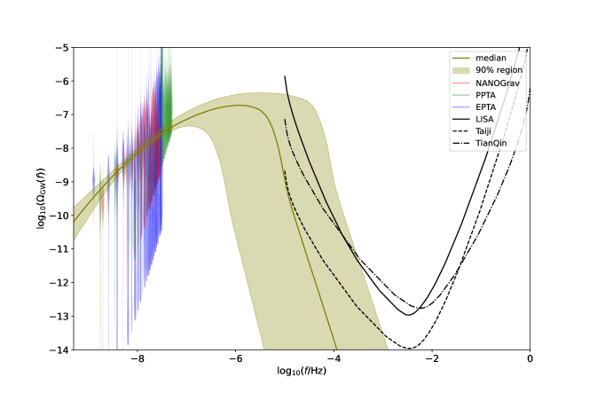
Figure 1: The posterior predictive distribution for the energy density from SIGWs for the $\mathcal{M}_{\mathrm{NG}}$ model. The solid olive line is the median value, while the shaded region represents the $90\%$ credible region. We also show the energy density spectra derived from the free spectrum from NANOGrav 15-yr data set (red violins), PPTA DR3 (green violins), and EPTA DR2 (blue violins). The black solid, dashed, and dash-dotted lines represent the power-law integrated sensitivity curves for LISA, Taiji, and TianQin, respectively.

Parameter	$A$	$\Delta$	$f_{*}/\mathrm{Hz}$	$|F_{\mathrm{NL}}|$
Prior	log-${\mathcal{U}}(-3,2)$	${\mathcal{U}}(0.05,5)$	log-${\mathcal{U}}(-9,-2)$	log-${\mathcal{U}}(-5,3)$
Result for $\mathcal{M}_{\mathrm{G}}$	$1.73^{+5.57}_{-1.47}$	$3.24^{+0.70}_{-1.34}$	$3.25^{+51.1}_{-3.22}\times 10^{-5}$	–
Result for $\mathcal{M}_{\mathrm{NG}}$	$1.06^{+5.20}_{-1.02}$	$3.36^{+1.10}_{-1.29}$	$1.81^{+45.3}_{-1.79}\times 10^{-5}$	$\lesssim 13.9$

Table 1: Prior distributions and results for the model parameters. We consider two cases: a model with non-Gaussianity, $\mathcal{M}_{\mathrm{NG}}$, and a model without non-Gaussianity, $\mathcal{M}_{\mathrm{G}}$. Here ${\mathcal{U}}$ and log-${\mathcal{U}}$ denote the uniform and log-uniform distributions, respectively. We quote each parameter’s median value and $90\%$ equal-tail credible interval.

We note that a positive value of $F_{\mathrm{NL}}$ will increase the abundance of PBHs for a given power spectrum of curvature perturbations. Conversely, a negative value of $F_{\mathrm{NL}}$ will decrease the abundance of PBHs. This behavior highlights the impact of non-Gaussianity, quantified by $F_{\mathrm{NL}}$, on the formation and abundance of PBHs. The Gaussian curvature perturbation $\mathcal{R}_{\mathrm{G}}$ can be determined by solving Eq. (1) as Byrnes et al. (2012); Young and Byrnes (2013)

$$\mathcal{R}_{\mathrm{G}}^{\pm}(\mathcal{R})=\frac{1}{2F_{\text{NL}}}\left(-1\pm\sqrt{1+4F_{\text{NL}}\mathcal{R}+4F_{\text{NL}}^{2}\langle\mathcal{R}_{\mathrm{G}}^{2}\rangle}\right).$$ (12)

PBHs are expected to form when the curvature perturbation exceeds a certain threshold value $\mathcal{R}_{\mathrm{c}}\sim 1$ Musco et al. (2005, 2009); Musco and Miller (2013); Harada et al. (2013). The PBH mass fraction at formation time can be calculated as Young and Byrnes (2013)

$$\beta(M)\simeq\frac{1}{2}\!\left\{\begin{array}[]{cl}\!\!\!\operatorname{erfc}\!\!\left(\frac{\mathcal{R}_{\mathrm{G}}^{+}\left(\mathcal{R}_{\mathrm{c}}\right)}{\sqrt{2\left\langle\mathcal{R}_{\mathrm{G}}^{2}\right\rangle}}\right)+\operatorname{erfc}\!\!\left(-\frac{\mathcal{R}_{\mathrm{G}}^{-}\left(\mathcal{R}_{\mathrm{c}}\right)}{\sqrt{2\left\langle\mathcal{R}_{\mathrm{G}}^{2}\right\rangle}}\right);&F_{\mathrm{NL}}>0,\\ \!\!\operatorname{erf}\!\!\left(\frac{\mathcal{R}_{\mathrm{G}}^{+}\left(\mathcal{R}_{\mathrm{c}}\right)}{\sqrt{2\left\langle\mathcal{R}_{\mathrm{G}}^{2}\right\rangle}}\right)-\operatorname{erf}\!\!\left(\frac{\mathcal{R}_{\mathrm{G}}^{-}\left(\mathcal{R}_{\mathrm{c}}\right)}{\sqrt{2\left\langle\mathcal{R}_{\mathrm{G}}^{2}\right\rangle}}\right);&F_{\mathrm{NL}}<0.\end{array}\right.$$ (13)

One can define the total abundance of PBHs in the dark matter at present as Sasaki et al. (2018)

$$f_{\mathrm{PBH}} \equiv\frac{\Omega_{\mathrm{PBH}}}{\Omega_{\mathrm{CDM}}}=2.7\times 10^{8}\int_{-\infty}^{\infty}\mathrm{d}\ln M$$ (14)

$$\times\left(\frac{g_{*,r}}{10.75}\right)^{3/4}\left(\frac{g_{*,s}}{10.75}\right)^{-1}\left(\frac{M}{M_{\odot}}\right)^{-1/2}\beta(M),$$

where $\Omega_{\mathrm{CDM}}$ is the cold dark matter density.

Data analyses and results. We jointly use the NANOGrav 15-yr data set, PPTA DR3, and EPTA DR2 to estimate the model parameters. The ongoing efforts of these PTAs have lasted for more than a decade. Specifically, the NANOGrav 15-yr data set contains observations of $68$ pulsars with a time span of $16.03$ years Agazie et al. (2023a), PPTA DR3 contains observations of $32$ pulsars with a time span of up to $18$ years Zic et al. (2023), and EPTA DR2 contains observations of $25$ pulsars with a time span of $24.7$ years Antoniadis et al. (2023a). These PTA data sets all present a stochastic signal consistent with the Hellings-Downs spatial correlations expected for an SGWB. If this signal is indeed of GW origin, it should share the same properties among these PTAs. Therefore, we combine the observations from these PTAs to estimate model parameters to increase the precision rather than using each individual PTA. In this letter, we use the free spectrum amplitude derived by each PTA with Hellings-Downs correlations. Given the time span $T_{\mathrm{obs}}$ of a PTA, the free spectrum starts with the lowest frequency $1/T_{\mathrm{obs}}$. NANOGrav, PPTA, and EPTA use $14$, $28$, and $24$ frequency components in their SGWB searches, respectively. Combining these data together results in $66$ frequencies of a free spectrum ranging from $1.28$ nHz to $49.1$ nHz. A visualization of the data used in the analyses is shown in Fig. 1. In this work, we also consider the constraint from baryon acoustic oscillation and CMB Aghanim et al. (2020b) for the integrated energy-density fraction that $\int_{k_{\min}}^{\infty}h^{2}\Omega_{\mathrm{GW},0}(k)\,d\ln k\lesssim 2.9\times 10^{-7}$ Clarke et al. (2020), where $h=H_{0}/(100\mathrm{km}\,\mathrm{s}^{-1}\,\mathrm{Mpc}^{-1})=0.674$ Aghanim et al. (2020b) is the dimensionless Hubble constant.

We use the time delay data released by each PTA. The time delay $d(f)$ can be converted to the power spectrum $S(f)$ by

$$d(f)=\sqrt{S(f)/T_{\mathrm{obs}}}.$$ (15)

We then convert $S(f)$ to the characteristic strain, $h_{c}(f)$, by

$$h_{c}^{2}(f)=12\pi^{2}f^{3}S(f).$$ (16)

Further, we obtain the free spectrum energy density as

$$\hat{\Omega}_{\mathrm{GW}}(f)=\frac{2\pi^{2}}{3H_{0}^{2}}f^{2}h_{c}^{2}(f)=\frac{8\pi^{4}}{H_{0}^{2}}T_{\mathrm{obs}}f^{5}d^{2}(f).$$ (17)

For each frequency $f_{i}$, with the posteriors of $\hat{\Omega}_{\mathrm{GW}}(f_{i})$ at hand, we can estimate the corresponding kernel density $\mathcal{L}_{i}$. Therefore, the total likelihood is

$$\mathcal{L}(\Lambda)=\prod_{i=1}^{66}\mathcal{L}_{i}(\Omega_{\mathrm{GW}}(f_{i},\Lambda)),$$ (18)

where $\Lambda\equiv\{A,\Delta,f_{*},|F_{\mathrm{NL}}|\}$ is the collection of the model parameters. We use dynesty Speagle (2020) sampler wrapped in Bilby Ashton et al. (2019); Romero-Shaw et al. (2020) package to search over the parameter space. The model parameters and their priors are summarized in Table 1.

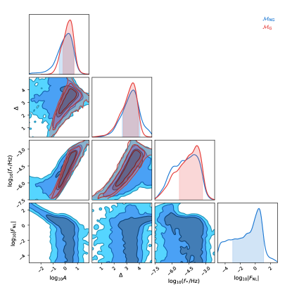
Figure 2: One and two-dimensional marginalized posteriors of the parameters for the $\mathcal{M}_{\mathrm{G}}$ (red) model and the $\mathcal{M}_{\mathrm{NG}}$ (blue) model. We jointly use the PTA data from the NANOGrav 15-yr data set, PPTA DR3, and EPTA DR2. The contours in the two-dimensional plot correspond to the $1\sigma$, $2\sigma$, and $3\sigma$ credible regions, respectively.

We consider two models: one without non-Gaussianity, $\mathcal{M}_{\mathrm{G}}$, and another with non-Gaussianity, $\mathcal{M}_{\mathrm{NG}}$. The posterior distributions for the parameters are shown in Fig. 2, and the median and $90\%$ credible interval values for each parameter are summarized in Table 1. We note that the $\mathcal{M}_{\mathrm{G}}$ model has been studied by NANOGrav with their 15-yr data set, which is called SIGW-GAUSS in their paper. While we obtain consistent results, the combined data from NANOGrav, PPTA, and EPTA can constrain the parameters to higher precision than using the NANOGrav data set alone, as expected. For the $\mathcal{M}_{\mathrm{NG}}$ model, the $F_{\mathrm{NL}}$ and $A$ parameters are generally degenerate. The combined data can constrain the amplitude to be $A=1.06^{+5.20}_{-1.02}$, therefore constraining $|F_{\mathrm{NL}}|\lesssim 13.9$. Since positive and negative $F_{\mathrm{NL}}$ values are degenerate, we have $-13.9\lesssim F_{\mathrm{NL}}\lesssim 13.9$. Moreover, the abundance of PBHs cannot exceed that of dark matter, i.e., $f_{\mathrm{PBH}}\lesssim 1$. Using Eqs. (13) and (14), this limitation allows us to break the degeneracy and obtain constraints on $F_{\mathrm{NL}}$ as $-13.9\lesssim F_{\mathrm{NL}}\lesssim-0.1$.

Summary and discussion. While the CMB and large-scale structure observations have provided increasingly precise measurements on the largest scales of the Universe, our knowledge of small scales remains limited, except for the constraints imposed by PBHs. PTAs, on the other hand, are an invaluable tool to probe the small-scale non-Gaussianity through SIGWs. Assuming the stochastic signal detected by the PTA collaborations originates from SIGWs, we jointly use the NANOGrav 15-yr data set, PPTA DR3, and EPTA DR2 to constrain the SIGWs accounting for non-Gaussianity. For the first time, we constrain the non-linear parameter as $|F_{\mathrm{NL}}|\lesssim 13.9$ for a lognormal power spectrum of the curvature perturbation. Furthermore, we obtain $-13.9\lesssim F_{\mathrm{NL}}\lesssim-0.1$ to avoid overproduction of PBHs. Although we have only dealt with the lognormal power spectrum of curvature perturbations, the method and the framework proposed in this work can be easily extended to different types of power spectra. For instance, a similar constraint on the non-Gaussianity parameter associated with the broken power-law spectrum is presented in the Supplementary Material.

The constraints on primordial non-Gaussianity of local type have significant implications for inflation models that involve scalar fields, other than the inflaton, in generating the primordial curvature perturbations. For instance, adiabatic curvaton models predict that Bartolo et al. (2004b, 2010)

$$f_{\mathrm{NL}}=\frac{5}{3}F_{\mathrm{NL}}=\frac{5}{4r_{\mathrm{D}}}-\frac{5r_{\mathrm{D}}}{6}-\frac{5}{3},$$ (19)

when the curvaton field has a quadratic potential Lyth and Wands (2002); Lyth et al. (2003); Lyth and Rodriguez (2005); Malik and Lyth (2006); Sasaki et al. (2006). Here the parameter $r_{\mathrm{D}}=3\rho_{\mathrm{curvaton}}/(3\rho_{\mathrm{curvaton}}+4\rho_{\mathrm{radiation}})$ represents the “curvaton decay fraction” at the time of curvaton decay under sudden decay approximation. Our constraint $|F_{\mathrm{NL}}|\lesssim 13.9$ implies

$$r_{\mathrm{D}}\gtrsim 0.05\quad(95\%),$$ (20)

and the further constraint that $F_{\mathrm{NL}}\lesssim-0.1$ yields

$$r_{\mathrm{D}}\gtrsim 0.62\quad(95\%),$$ (21)

indicating that the curvaton field has a non-negligible energy density when it decays. Our findings, therefore, pave the way to constrain inflation models with PTA data.

Furthermore, as indicated in Fig. 1, the energy density spectrum of SIGW can generally be extended to the frequency band of the space-borne GW detector. Therefore, the multi-band observations of PTAs with the forthcoming space-borne GW detectors, such as LISA/Taiji/TianQin, will provide a complementary investigation of non-Gaussianity.

Note added. While finalizing this work, we found two parallel independent studies Franciolini et al. (2023); Wang et al. (2023) that also explore the potential connection between the NANOGrav signal and SIGWs associated with non-Gaussianity. In particular, Ref. Franciolini et al. (2023) focused on the significance of the non-Gaussianity parameter to address the issue of PBH overproduction; however, it did not constrain the non-Gaussianity parameter with PTA data. On the other hand, Ref. Wang et al. (2023) did obtain a constraint on the non-Gaussianity parameter with the NANOGrav data, but it is noteworthy that Ref. Wang et al. (2023) adopted a less rigorous approach by manually fixing other model parameters. In contrast, our approach employs a comprehensive Bayesian inference methodology, providing a rigorous constraint on the non-Gaussianity parameter using multiple PTA data sets.

Acknowledgments. The contour plots are generated with ChainConsumer Hinton (2016). LL is supported by the National Natural Science Foundation of China (Grant No. 12247112 and No. 12247176) and the China Postdoctoral Science Foundation Fellowship No. 2023M730300. ZCC is supported by the National Natural Science Foundation of China (Grant No. 12247176 and No. 12247112) and the China Postdoctoral Science Foundation Fellowship No. 2022M710429. QGH is supported by grants from NSFC (Grant No. 12250010, 11975019, 11991052, 12047503), Key Research Program of Frontier Sciences, CAS, Grant No. ZDBS-LY-7009, CAS Project for Young Scientists in Basic Research YSBR-006, the Key Research Program of the Chinese Academy of Sciences (Grant No. XDPB15).

I Impact of non-Gaussianity on PBH abundance

We consider the model of local quadratic non-Gaussianity as Verde et al. (2000, 2001); Komatsu and Spergel (2001); Bartolo et al. (2004a); Boubekeur and Lyth (2006); Byrnes et al. (2007)

$$\mathcal{R}(\vec{x})=\mathcal{R}_{\mathrm{G}}(\vec{x})+F_{\mathrm{NL}}\left(\mathcal{R}_{\mathrm{G}}^{2}(\vec{x})-\left\langle\mathcal{R}_{\mathrm{G}}^{2}(\vec{x})\right\rangle\right),$$ (S1)

where $\mathcal{R}_{\mathrm{G}}({\vec{x}})$ follows Gaussian statistics and the term $\left\langle\mathcal{R}_{\mathrm{G}}^{2}\right\rangle$ is included to ensure that the expectation value for the curvature perturbations remains zero, $\langle\mathcal{R}\rangle=0$. Solving this equation to find $\mathcal{R}_{G}$ as a function of $\mathcal{R}$ gives two solutions Byrnes et al. (2012); Young and Byrnes (2013)

$$\mathcal{R}_{\mathrm{G}}^{\pm}(\mathcal{R})=\frac{1}{2F_{\text{NL}}}\left(-1\pm\sqrt{1+4F_{\text{NL}}\mathcal{R}+4F_{\text{NL}}^{2}\langle\mathcal{R}_{\mathrm{G}}^{2}\rangle}\right).$$ (S2)

Making a formal change of variable, we can achieve the non-Gaussian probability distribution function as

$$P_{\mathrm{NG}}(\mathcal{R})d\mathcal{R}=\sum_{i=\pm}\left|\frac{d\mathcal{R}_{\mathrm{G}}^{i}(\mathcal{R})}{d\mathcal{R}}\right|P_{\mathrm{G}}\left(\mathcal{R}_{\mathrm{G}}^{i}(\mathcal{R})\right)d\mathcal{R},$$ (S3)

where

$$P_{\mathrm{G}}(\mathcal{R})=\frac{1}{\sqrt{2\pi\left\langle\mathcal{R}_{\mathrm{G}}^{2}(\vec{x})\right\rangle}}\exp\left(-\frac{1}{2}\frac{\mathcal{R}^{2}}{\left\langle\mathcal{R}_{\mathrm{G}}^{2}(\vec{x})\right\rangle}\right)$$ (S4)

is the Gaussian probability distribution function. The PBH mass fraction at formation time is given by

$$\beta\simeq\int_{\mathcal{R}_{c}}^{\mathcal{R}_{\rm max}}P_{\rm NG}(\mathcal{R})d\mathcal{R}.$$ (S5)

When $F_{\rm NL}$ is positive (or zero), $\mathcal{R}_{\rm max}=\infty$. However, if $F_{\rm NL}$ is negative, then $\mathcal{R}$ is bounded from Eq. (S2). In this case, $\mathcal{R}_{\rm max}$ is given by the expression Young and Byrnes (2013)

$$\mathcal{R}_{\rm max}=-\frac{1}{4F_{\rm NL}}\left(1+4F_{\rm NL}^{2}\langle\mathcal{R}_{\mathrm{G}}^{2}\rangle\right).$$ (S6)

Fig. S1 illustrates the impact of the non-Gaussianity parameter $F_{\mathrm{NL}}$ on the probability distribution of the curvature perturbation $\mathcal{R}$. The primary effect of $F_{\rm NL}$ is to skew the distribution of $\mathcal{R}$. When $F_{\rm NL}$ is positive, we observe a peak in the distribution for negative values of $\mathcal{R}$, along with a large tail for positive values of $\mathcal{R}$. Conversely, for negative $F_{\rm NL}$, we observe a peak in the distribution for positive values of $\mathcal{R}$, along with a small tail for positive values of $\mathcal{R}$. If the maximum curvature perturbation $\mathcal{R}_{\rm max}$ satisfies $\mathcal{R}_{\rm max}<\mathcal{R}_{c}$, then no PBH formation would be expected for these values. In summary, a positive value of $F_{\mathrm{NL}}$ will increase the abundance of PBHs, while a negative value of $F_{\mathrm{NL}}$ will decrease the abundance of PBHs. From Eq. (S5), for $F_{\rm NL}>0$, we have

$$\beta\simeq\frac{1}{2}\left[\operatorname{erfc}\!\!\left(\frac{\mathcal{R}_{\mathrm{G}}^{+}\left(\mathcal{R}_{\mathrm{c}}\right)}{\sqrt{2\left\langle\mathcal{R}_{\mathrm{G}}^{2}\right\rangle}}\right)+\operatorname{erfc}\!\!\left(-\frac{\mathcal{R}_{\mathrm{G}}^{-}\left(\mathcal{R}_{\mathrm{c}}\right)}{\sqrt{2\left\langle\mathcal{R}_{\mathrm{G}}^{2}\right\rangle}}\right)\right],$$ (S7)

and $F_{\rm NL}<0$, we have

$$\beta\simeq\frac{1}{2}\left[\operatorname{erf}\!\!\left(\frac{\mathcal{R}_{\mathrm{G}}^{+}\left(\mathcal{R}_{\mathrm{c}}\right)}{\sqrt{2\left\langle\mathcal{R}_{\mathrm{G}}^{2}\right\rangle}}\right)-\operatorname{erf}\!\!\left(\frac{\mathcal{R}_{\mathrm{G}}^{-}\left(\mathcal{R}_{\mathrm{c}}\right)}{\sqrt{2\left\langle\mathcal{R}_{\mathrm{G}}^{2}\right\rangle}}\right)\right].$$ (S8)

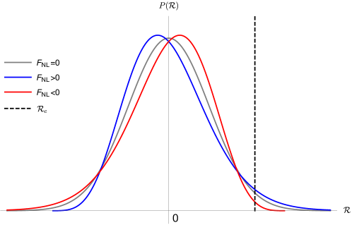
Figure S1: An illustration of the impact of the non-Gaussianity parameter $F_{\mathrm{NL}}$ on the probability distribution of the curvature perturbation $\mathcal{R}$. Notably, non-Gaussianity induces a skew in the distribution. A positive $F_{\mathrm{NL}}$ extends the tail of the probability distribution for $\mathcal{R}>0$, thereby elevating the likelihood of $\mathcal{R}>\mathcal{R}_{c}$ and consequently leading to increased production of PBHs. Conversely, a negative $F_{\mathrm{NL}}$ diminishes the PBH production.

II Broken power-law spectrum

Here, we consider another curvature perturbation spectrum characterized by a broken power-law form. The broken power-law spectrum can describe a common class of spectra that exhibit peaks, often associated with single-field inflation or curvaton models. The functional form is given by

$$\mathcal{P}^{\rm BPL}_{\mathcal{R}}(k)=A\frac{\left(\alpha+\beta\right)^{\gamma}}{\left[\beta\left(k/k_{*}\right)^{-\alpha/\gamma}+\alpha\left(k/k_{*}\right)^{\beta/\gamma}\right]^{\gamma}}.$$ (S9)

Here, $\alpha$ and $\beta$ are both positive numbers that describe the growth and decay of the spectrum around the peak, respectively. The parameter $\gamma$ characterizes the flatness of the peak, with typical values for $\alpha$ being $\alpha\lesssim 4$ Byrnes et al. (2019). Additionally, in quasi-inflection-point models that give rise to stellar-mass PBHs, one typically expects $\beta\gtrsim 0.5$, while for curvaton models $\beta\gtrsim 2$.

Parameter	$f_{*}/\mathrm{Hz}$	$A$	$\alpha$	$\beta$	$\gamma$	$|F_{\mathrm{NL}}|$
Prior	log-${\mathcal{U}}(-9,-2)$	log-${\mathcal{U}}(-3,2)$	${\mathcal{U}}(0,2)$	${\mathcal{U}}(0,10)$	${\mathcal{U}}(0,10)$	log-${\mathcal{U}}(-5,4)$
Result for $\mathcal{M}_{\mathrm{G}}$	$3.2^{+12.3}_{-2.5}\times 10^{-7}$	$0.82^{+0.58}_{-0.37}$	$0.86^{+0.76}_{-0.21}$	$4.6^{+4.8}_{-3.60}$	$4.9^{+4.6}_{-4.2}$	–
Result for $\mathcal{M}_{\mathrm{NG}}$	$2.7^{+9.8}_{-2.1}\times 10^{-7}$	$0.67^{+0.67}_{-0.65}$	$0.83^{+0.79}_{-0.30}$	$4.8^{+4.50}_{-3.7}$	$5.1^{+4.4}_{-4.4}$	$\lesssim 11.1$

Table S1: Same as Table 1, but for the broken power-law spectrum.

The model parameters, along with their priors and inferred values are summarized in Table S1, while the posterior distributions for the parameters are shown in Fig. S2. The joint analysis, incorporating the NANOGrav 15-yr data set, PPTA DR3, and EPTA DR2, yields the constraint: $-11.1\lesssim F_{\mathrm{NL}}\lesssim 11.1$. To avoid the PBH overproduction, we further constrain the non-Guassianity parameter as $-11.1\lesssim F_{\mathrm{NL}}\lesssim-0.3$.

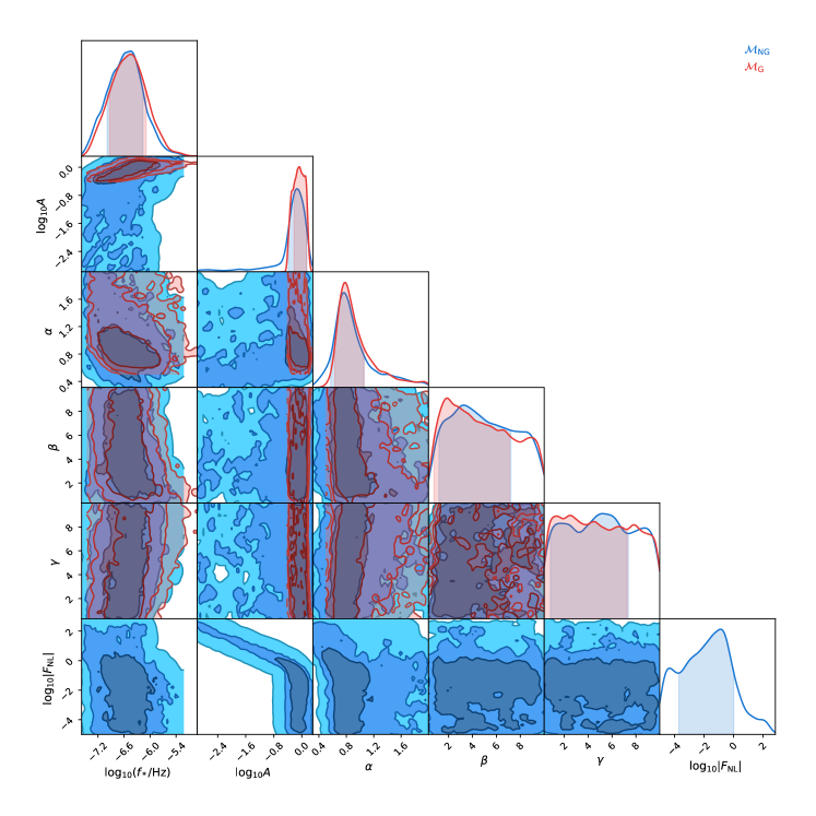
Figure S2: Same as Fig. 2, but for the broken power-law spectrum.

References

- Armendariz-Picon et al. (1999) C. Armendariz-Picon, T. Damour, and V. F. Mukhanov, Phys. Lett. B 458, 209 (1999), arXiv:hep-th/9904075 .
- Garriga and Mukhanov (1999) J. Garriga and V. F. Mukhanov, Phys. Lett. B 458, 219 (1999), arXiv:hep-th/9904176 .
- Kobayashi et al. (2010) T. Kobayashi, M. Yamaguchi, and J. Yokoyama, Phys. Rev. Lett. 105, 231302 (2010), arXiv:1008.0603 [hep-th] .
- Arkani-Hamed et al. (2004) N. Arkani-Hamed, H.-C. Cheng, M. A. Luty, and S. Mukohyama, JHEP 05, 074 (2004), arXiv:hep-th/0312099 .
- Alishahiha et al. (2004) M. Alishahiha, E. Silverstein, and D. Tong, Phys. Rev. D 70, 123505 (2004), arXiv:hep-th/0404084 .
- Baumann et al. (2016) D. Baumann, H. Lee, and G. L. Pimentel, JHEP 01, 101 (2016), arXiv:1507.07250 [hep-th] .
- Seery and Lidsey (2005) D. Seery and J. E. Lidsey, JCAP 06, 003 (2005), arXiv:astro-ph/0503692 .
- Kobayashi et al. (2011) T. Kobayashi, M. Yamaguchi, and J. Yokoyama, Phys. Rev. D 83, 103524 (2011), arXiv:1103.1740 [hep-th] .
- Baumann and Green (2011) D. Baumann and D. Green, JCAP 09, 014 (2011), arXiv:1102.5343 [hep-th] .
- Baumann and Green (2012) D. Baumann and D. Green, Phys. Rev. D 85, 103520 (2012), arXiv:1109.0292 [hep-th] .
- Kristiano and Yokoyama (2022) J. Kristiano and J. Yokoyama, Phys. Rev. Lett. 128, 061301 (2022), arXiv:2104.01953 [hep-th] .
- Aghanim et al. (2020a) N. Aghanim et al. (Planck), Astron. Astrophys. 641, A5 (2020a), arXiv:1907.12875 [astro-ph.CO] .
- Alam et al. (2021) S. Alam et al. (eBOSS), Phys. Rev. D 103, 083533 (2021), arXiv:2007.08991 [astro-ph.CO] .
- Pandey et al. (2022) S. Pandey et al. (DES), Phys. Rev. D 106, 043520 (2022), arXiv:2105.13545 [astro-ph.CO] .
- Amaro-Seoane et al. (2017) P. Amaro-Seoane et al. (LISA), (2017), arXiv:1702.00786 [astro-ph.IM] .
- Ruan et al. (2020) W.-H. Ruan, Z.-K. Guo, R.-G. Cai, and Y.-Z. Zhang, Int. J. Mod. Phys. A 35, 2050075 (2020), arXiv:1807.09495 [gr-qc] .
- Luo et al. (2016) J. Luo et al. (TianQin), Class. Quant. Grav. 33, 035010 (2016), arXiv:1512.02076 [astro-ph.IM] .
- Tomita (1967) K. Tomita, Progress of Theoretical Physics 37, 831 (1967).
- Saito and Yokoyama (2009) R. Saito and J. Yokoyama, Phys. Rev. Lett. 102, 161101 (2009), [Erratum: Phys.Rev.Lett. 107, 069901 (2011)], arXiv:0812.4339 [astro-ph] .
- Young et al. (2014) S. Young, C. T. Byrnes, and M. Sasaki, JCAP 07, 045 (2014), arXiv:1405.7023 [gr-qc] .
- Cai et al. (2019a) R.-g. Cai, S. Pi, and M. Sasaki, Phys. Rev. Lett. 122, 201101 (2019a), arXiv:1810.11000 [astro-ph.CO] .
- Cai et al. (2019b) R.-G. Cai, S. Pi, S.-J. Wang, and X.-Y. Yang, JCAP 10, 059 (2019b), arXiv:1907.06372 [astro-ph.CO] .
- Kohri and Terada (2018) K. Kohri and T. Terada, Phys. Rev. D 97, 123532 (2018), arXiv:1804.08577 [gr-qc] .
- Yuan et al. (2019) C. Yuan, Z.-C. Chen, and Q.-G. Huang, Phys. Rev. D 100, 081301 (2019), arXiv:1906.11549 [astro-ph.CO] .
- Yuan et al. (2020a) C. Yuan, Z.-C. Chen, and Q.-G. Huang, Phys. Rev. D 101, 043019 (2020a), arXiv:1910.09099 [astro-ph.CO] .
- Chen et al. (2020) Z.-C. Chen, C. Yuan, and Q.-G. Huang, Phys. Rev. Lett. 124, 251101 (2020), arXiv:1910.12239 [astro-ph.CO] .
- Yuan et al. (2020b) C. Yuan, Z.-C. Chen, and Q.-G. Huang, Phys. Rev. D 101, 063018 (2020b), arXiv:1912.00885 [astro-ph.CO] .
- Sazhin (1978) M. V. Sazhin, Soviet Astronomy 22, 36 (1978).
- Detweiler (1979) S. L. Detweiler, Astrophys. J. 234, 1100 (1979).
- Agazie et al. (2023a) G. Agazie et al. (NANOGrav), Astrophys. J. Lett. 951, L9 (2023a), arXiv:2306.16217 [astro-ph.HE] .
- Agazie et al. (2023b) G. Agazie et al. (NANOGrav), Astrophys. J. Lett. 951, L8 (2023b), arXiv:2306.16213 [astro-ph.HE] .
- Zic et al. (2023) A. Zic et al., Publ. Astron. Soc. Austral. 40, e049 (2023), arXiv:2306.16230 [astro-ph.HE] .
- Reardon et al. (2023) D. J. Reardon et al., Astrophys. J. Lett. 951, L6 (2023), arXiv:2306.16215 [astro-ph.HE] .
- Antoniadis et al. (2023a) J. Antoniadis et al. (EPTA), Astron. Astrophys. 678, A48 (2023a), arXiv:2306.16224 [astro-ph.HE] .
- Antoniadis et al. (2023b) J. Antoniadis et al. (EPTA, InPTA:), Astron. Astrophys. 678, A50 (2023b), arXiv:2306.16214 [astro-ph.HE] .
- Xu et al. (2023) H. Xu et al., Res. Astron. Astrophys. 23, 075024 (2023), arXiv:2306.16216 [astro-ph.HE] .
- Hellings and Downs (1983) R. w. Hellings and G. s. Downs, Astrophys. J. Lett. 265, L39 (1983).
- Li et al. (2019) J. Li, Z.-C. Chen, and Q.-G. Huang, Sci. China Phys. Mech. Astron. 62, 110421 (2019), [Erratum: Sci.China Phys.Mech.Astron. 64, 250451 (2021)], arXiv:1907.09794 [astro-ph.CO] .
- Vagnozzi (2021) S. Vagnozzi, Mon. Not. Roy. Astron. Soc. 502, L11 (2021), arXiv:2009.13432 [astro-ph.CO] .
- Chen et al. (2021) Z.-C. Chen, C. Yuan, and Q.-G. Huang, Sci. China Phys. Mech. Astron. 64, 120412 (2021), arXiv:2101.06869 [astro-ph.CO] .
- Wu et al. (2022a) Y.-M. Wu, Z.-C. Chen, and Q.-G. Huang, Astrophys. J. 925, 37 (2022a), arXiv:2108.10518 [astro-ph.CO] .
- Chen et al. (2022a) Z.-C. Chen, Y.-M. Wu, and Q.-G. Huang, Commun. Theor. Phys. 74, 105402 (2022a), arXiv:2109.00296 [astro-ph.CO] .
- Benetti et al. (2022) M. Benetti, L. L. Graef, and S. Vagnozzi, Phys. Rev. D 105, 043520 (2022), arXiv:2111.04758 [astro-ph.CO] .
- Chen et al. (2022b) Z.-C. Chen, Y.-M. Wu, and Q.-G. Huang, Astrophys. J. 936, 20 (2022b), arXiv:2205.07194 [astro-ph.CO] .
- Ashoorioon et al. (2022) A. Ashoorioon, K. Rezazadeh, and A. Rostami, Phys. Lett. B 835, 137542 (2022), arXiv:2202.01131 [astro-ph.CO] .
- Wu et al. (2022b) Y.-M. Wu, Z.-C. Chen, Q.-G. Huang, X. Zhu, N. D. R. Bhat, Y. Feng, G. Hobbs, R. N. Manchester, C. J. Russell, and R. M. Shannon (PPTA), Phys. Rev. D 106, L081101 (2022b), arXiv:2210.03880 [astro-ph.CO] .
- Wu et al. (2023a) Y.-M. Wu, Z.-C. Chen, and Q.-G. Huang, Phys. Rev. D 107, 042003 (2023a), arXiv:2302.00229 [gr-qc] .
- Falxa et al. (2023) M. Falxa et al. (IPTA), Mon. Not. Roy. Astron. Soc. 521, 5077 (2023), arXiv:2303.10767 [gr-qc] .
- Wu et al. (2023b) Y.-M. Wu, Z.-C. Chen, and Q.-G. Huang, JCAP 09, 021 (2023b), arXiv:2305.08091 [hep-ph] .
- Dandoy et al. (2023) V. Dandoy, V. Domcke, and F. Rompineve, SciPost Phys. Core 6, 060 (2023), arXiv:2302.07901 [astro-ph.CO] .
- Madge et al. (2023) E. Madge, E. Morgante, C. Puchades-Ibáñez, N. Ramberg, W. Ratzinger, S. Schenk, and P. Schwaller, JHEP 10, 171 (2023), arXiv:2306.14856 [hep-ph] .
- Afzal et al. (2023) A. Afzal et al. (NANOGrav), Astrophys. J. Lett. 951, L11 (2023), arXiv:2306.16219 [astro-ph.HE] .
- Antoniadis et al. (2023c) J. Antoniadis et al. (EPTA), (2023c), arXiv:2306.16227 [astro-ph.CO] .
- King et al. (2023) S. F. King, D. Marfatia, and M. H. Rahat, (2023), arXiv:2306.05389 [hep-ph] .
- Niu and Rahat (2023) X. Niu and M. H. Rahat, Phys. Rev. D 108, 115023 (2023), arXiv:2307.01192 [hep-ph] .
- Datta and Samanta (2023) S. Datta and R. Samanta, Phys. Rev. D 108, L091706 (2023), arXiv:2307.00646 [hep-ph] .
- Vagnozzi (2023) S. Vagnozzi, JHEAp 39, 81 (2023), arXiv:2306.16912 [astro-ph.CO] .
- Bi et al. (2023) Y.-C. Bi, Y.-M. Wu, Z.-C. Chen, and Q.-G. Huang, Sci. China Phys. Mech. Astron. 66, 120402 (2023), arXiv:2307.00722 [astro-ph.CO] .
- Wu et al. (2023c) Y.-M. Wu, Z.-C. Chen, and Q.-G. Huang, (2023c), arXiv:2307.03141 [astro-ph.CO] .
- Jin et al. (2023) J.-H. Jin, Z.-C. Chen, Z. Yi, Z.-Q. You, L. Liu, and Y. Wu, JCAP 09, 016 (2023), arXiv:2307.08687 [astro-ph.CO] .
- Liu et al. (2023a) L. Liu, Z.-C. Chen, and Q.-G. Huang, JCAP 11, 071 (2023a), arXiv:2307.14911 [astro-ph.CO] .
- Yi et al. (2023a) Z. Yi, Z.-Q. You, Y. Wu, Z.-C. Chen, and L. Liu, (2023a), arXiv:2308.14688 [astro-ph.CO] .
- Agazie et al. (2023c) G. Agazie et al. (International Pulsar Timing Array), (2023c), arXiv:2309.00693 [astro-ph.HE] .
- Yi et al. (2023b) Z. Yi, Z.-Q. You, and Y. Wu, (2023b), arXiv:2308.05632 [astro-ph.CO] .
- You et al. (2023) Z.-Q. You, Z. Yi, and Y. Wu, JCAP 11, 065 (2023), arXiv:2307.04419 [gr-qc] .
- Chen et al. (2023a) Z.-C. Chen, Q.-G. Huang, C. Liu, L. Liu, X.-J. Liu, Y. Wu, Y.-M. Wu, Z. Yi, and Z.-Q. You, (2023a), arXiv:2310.00411 [astro-ph.IM] .
- Zel’dovich and Novikov (1967) Y. B. Zel’dovich and I. D. Novikov, Sov. Astron. 10, 602 (1967).
- Hawking (1971) S. Hawking, Mon. Not. Roy. Astron. Soc. 152, 75 (1971).
- Carr and Hawking (1974) B. J. Carr and S. W. Hawking, Mon. Not. Roy. Astron. Soc. 168, 399 (1974).
- Belotsky et al. (2014) K. M. Belotsky, A. D. Dmitriev, E. A. Esipova, V. A. Gani, A. V. Grobov, M. Y. Khlopov, A. A. Kirillov, S. G. Rubin, and I. V. Svadkovsky, Mod. Phys. Lett. A 29, 1440005 (2014), arXiv:1410.0203 [astro-ph.CO] .
- Carr et al. (2016) B. Carr, F. Kuhnel, and M. Sandstad, Phys. Rev. D 94, 083504 (2016), arXiv:1607.06077 [astro-ph.CO] .
- Garcia-Bellido and Ruiz Morales (2017) J. Garcia-Bellido and E. Ruiz Morales, Phys. Dark Univ. 18, 47 (2017), arXiv:1702.03901 [astro-ph.CO] .
- Carr et al. (2017) B. Carr, M. Raidal, T. Tenkanen, V. Vaskonen, and H. Veermäe, Phys. Rev. D 96, 023514 (2017), arXiv:1705.05567 [astro-ph.CO] .
- Germani and Prokopec (2017) C. Germani and T. Prokopec, Phys. Dark Univ. 18, 6 (2017), arXiv:1706.04226 [astro-ph.CO] .
- Chen et al. (2019) Z.-C. Chen, F. Huang, and Q.-G. Huang, Astrophys. J. 871, 97 (2019), arXiv:1809.10360 [gr-qc] .
- Liu et al. (2019a) L. Liu, Z.-K. Guo, and R.-G. Cai, Phys. Rev. D 99, 063523 (2019a), arXiv:1812.05376 [astro-ph.CO] .
- Chen and Huang (2018) Z.-C. Chen and Q.-G. Huang, Astrophys. J. 864, 61 (2018), arXiv:1801.10327 [astro-ph.CO] .
- Liu et al. (2019b) L. Liu, Z.-K. Guo, and R.-G. Cai, Eur. Phys. J. C 79, 717 (2019b), arXiv:1901.07672 [astro-ph.CO] .
- Fu et al. (2019) C. Fu, P. Wu, and H. Yu, Phys. Rev. D 100, 063532 (2019), arXiv:1907.05042 [astro-ph.CO] .
- Liu et al. (2020a) J. Liu, Z.-K. Guo, and R.-G. Cai, Phys. Rev. D 101, 023513 (2020a), arXiv:1908.02662 [astro-ph.CO] .
- Cai et al. (2020) R.-G. Cai, Z.-K. Guo, J. Liu, L. Liu, and X.-Y. Yang, JCAP 06, 013 (2020), arXiv:1912.10437 [astro-ph.CO] .
- Chen and Huang (2020) Z.-C. Chen and Q.-G. Huang, JCAP 08, 039 (2020), arXiv:1904.02396 [astro-ph.CO] .
- Liu et al. (2020b) L. Liu, Z.-K. Guo, R.-G. Cai, and S. P. Kim, Phys. Rev. D 102, 043508 (2020b), arXiv:2001.02984 [astro-ph.CO] .
- Fu et al. (2020) C. Fu, P. Wu, and H. Yu, Phys. Rev. D 102, 043527 (2020), arXiv:2006.03768 [astro-ph.CO] .
- De Luca et al. (2021a) V. De Luca, V. Desjacques, G. Franciolini, P. Pani, and A. Riotto, Phys. Rev. Lett. 126, 051101 (2021a), arXiv:2009.01728 [astro-ph.CO] .
- Wu (2020) Y. Wu, Phys. Rev. D 101, 083008 (2020), arXiv:2001.03833 [astro-ph.CO] .
- Vaskonen and Veermäe (2021) V. Vaskonen and H. Veermäe, Phys. Rev. Lett. 126, 051303 (2021), arXiv:2009.07832 [astro-ph.CO] .
- De Luca et al. (2021b) V. De Luca, G. Franciolini, and A. Riotto, Phys. Rev. Lett. 126, 041303 (2021b), arXiv:2009.08268 [astro-ph.CO] .
- Domènech and Pi (2022) G. Domènech and S. Pi, Sci. China Phys. Mech. Astron. 65, 230411 (2022), arXiv:2010.03976 [astro-ph.CO] .
- Hütsi et al. (2021) G. Hütsi, M. Raidal, V. Vaskonen, and H. Veermäe, JCAP 03, 068 (2021), arXiv:2012.02786 [astro-ph.CO] .
- Chen et al. (2022c) Z.-C. Chen, C. Yuan, and Q.-G. Huang, Phys. Lett. B 829, 137040 (2022c), arXiv:2108.11740 [astro-ph.CO] .
- Kawai and Kim (2021) S. Kawai and J. Kim, Phys. Rev. D 104, 083545 (2021), arXiv:2108.01340 [astro-ph.CO] .
- Braglia et al. (2021) M. Braglia, J. Garcia-Bellido, and S. Kuroyanagi, JCAP 12, 012 (2021), arXiv:2110.07488 [astro-ph.CO] .
- Liu et al. (2023b) L. Liu, X.-Y. Yang, Z.-K. Guo, and R.-G. Cai, JCAP 01, 006 (2023b), arXiv:2112.05473 [astro-ph.CO] .
- Braglia et al. (2023) M. Braglia, J. Garcia-Bellido, and S. Kuroyanagi, Mon. Not. Roy. Astron. Soc. 519, 6008 (2023), arXiv:2201.13414 [astro-ph.CO] .
- Zheng et al. (2023) L.-M. Zheng, Z. Li, Z.-C. Chen, H. Zhou, and Z.-H. Zhu, Phys. Lett. B 838, 137720 (2023), arXiv:2212.05516 [astro-ph.CO] .
- Liu et al. (2023c) L. Liu, Z.-Q. You, Y. Wu, and Z.-C. Chen, Phys. Rev. D 107, 063035 (2023c), arXiv:2210.16094 [astro-ph.CO] .
- Meng et al. (2023) D.-S. Meng, C. Yuan, and Q.-G. Huang, Sci. China Phys. Mech. Astron. 66, 280411 (2023), arXiv:2212.03577 [astro-ph.CO] .
- Chen et al. (2023b) Z.-C. Chen, S. P. Kim, and L. Liu, Commun. Theor. Phys. 75, 065401 (2023b), arXiv:2210.15564 [gr-qc] .
- Chen et al. (2023c) Z.-C. Chen, S.-S. Du, Q.-G. Huang, and Z.-Q. You, JCAP 03, 024 (2023c), arXiv:2205.11278 [astro-ph.CO] .
- Guo et al. (2023) S.-Y. Guo, M. Khlopov, X. Liu, L. Wu, Y. Wu, and B. Zhu, (2023), arXiv:2306.17022 [hep-ph] .
- Sasaki et al. (2018) M. Sasaki, T. Suyama, T. Tanaka, and S. Yokoyama, Class. Quant. Grav. 35, 063001 (2018), arXiv:1801.05235 [astro-ph.CO] .
- Carr et al. (2021) B. Carr, K. Kohri, Y. Sendouda, and J. Yokoyama, Rept. Prog. Phys. 84, 116902 (2021), arXiv:2002.12778 [astro-ph.CO] .
- Carr and Kuhnel (2020) B. Carr and F. Kuhnel, Ann. Rev. Nucl. Part. Sci. 70, 355 (2020), arXiv:2006.02838 [astro-ph.CO] .
- Bird et al. (2016) S. Bird, I. Cholis, J. B. Muñoz, Y. Ali-Haïmoud, M. Kamionkowski, E. D. Kovetz, A. Raccanelli, and A. G. Riess, Phys. Rev. Lett. 116, 201301 (2016), arXiv:1603.00464 [astro-ph.CO] .
- Sasaki et al. (2016) M. Sasaki, T. Suyama, T. Tanaka, and S. Yokoyama, Phys. Rev. Lett. 117, 061101 (2016), [Erratum: Phys.Rev.Lett. 121, 059901 (2018)], arXiv:1603.08338 [astro-ph.CO] .
- Young and Byrnes (2013) S. Young and C. T. Byrnes, JCAP 08, 052 (2013), arXiv:1307.4995 [astro-ph.CO] .
- Unal (2019) C. Unal, Phys. Rev. D 99, 041301 (2019), arXiv:1811.09151 [astro-ph.CO] .
- Yuan and Huang (2021) C. Yuan and Q.-G. Huang, Phys. Lett. B 821, 136606 (2021), arXiv:2007.10686 [astro-ph.CO] .
- Adshead et al. (2021) P. Adshead, K. D. Lozanov, and Z. J. Weiner, JCAP 10, 080 (2021), arXiv:2105.01659 [astro-ph.CO] .
- Ragavendra (2022) H. V. Ragavendra, Phys. Rev. D 105, 063533 (2022), arXiv:2108.04193 [astro-ph.CO] .
- Garcia-Saenz et al. (2023) S. Garcia-Saenz, L. Pinol, S. Renaux-Petel, and D. Werth, JCAP 03, 057 (2023), arXiv:2207.14267 [astro-ph.CO] .
- Verde et al. (2000) L. Verde, L.-M. Wang, A. Heavens, and M. Kamionkowski, Mon. Not. Roy. Astron. Soc. 313, L141 (2000), arXiv:astro-ph/9906301 .
- Verde et al. (2001) L. Verde, R. Jimenez, M. Kamionkowski, and S. Matarrese, Mon. Not. Roy. Astron. Soc. 325, 412 (2001), arXiv:astro-ph/0011180 .
- Komatsu and Spergel (2001) E. Komatsu and D. N. Spergel, Phys. Rev. D 63, 063002 (2001), arXiv:astro-ph/0005036 .
- Bartolo et al. (2004a) N. Bartolo, E. Komatsu, S. Matarrese, and A. Riotto, Phys. Rept. 402, 103 (2004a), arXiv:astro-ph/0406398 .
- Boubekeur and Lyth (2006) L. Boubekeur and D. H. Lyth, Phys. Rev. D 73, 021301 (2006), arXiv:astro-ph/0504046 .
- Byrnes et al. (2007) C. T. Byrnes, K. Koyama, M. Sasaki, and D. Wands, JCAP 11, 027 (2007), arXiv:0705.4096 [hep-th] .
- Ferrante et al. (2023) G. Ferrante, G. Franciolini, A. Iovino, Junior., and A. Urbano, Phys. Rev. D 107, 043520 (2023), arXiv:2211.01728 [astro-ph.CO] .
- Byrnes et al. (2012) C. T. Byrnes, E. J. Copeland, and A. M. Green, Phys. Rev. D 86, 043512 (2012), arXiv:1206.4188 [astro-ph.CO] .
- Musco et al. (2005) I. Musco, J. C. Miller, and L. Rezzolla, Class. Quant. Grav. 22, 1405 (2005), arXiv:gr-qc/0412063 .
- Musco et al. (2009) I. Musco, J. C. Miller, and A. G. Polnarev, Class. Quant. Grav. 26, 235001 (2009), arXiv:0811.1452 [gr-qc] .
- Musco and Miller (2013) I. Musco and J. C. Miller, Class. Quant. Grav. 30, 145009 (2013), arXiv:1201.2379 [gr-qc] .
- Harada et al. (2013) T. Harada, C.-M. Yoo, and K. Kohri, Phys. Rev. D 88, 084051 (2013), [Erratum: Phys.Rev.D 89, 029903 (2014)], arXiv:1309.4201 [astro-ph.CO] .
- Aghanim et al. (2020b) N. Aghanim et al. (Planck), Astron. Astrophys. 641, A6 (2020b), [Erratum: Astron.Astrophys. 652, C4 (2021)], arXiv:1807.06209 [astro-ph.CO] .
- Clarke et al. (2020) T. J. Clarke, E. J. Copeland, and A. Moss, JCAP 10, 002 (2020), arXiv:2004.11396 [astro-ph.CO] .
- Speagle (2020) J. S. Speagle, Mon. Not. Roy. Astron. Soc. 493, 3132 (2020), arXiv:1904.02180 [astro-ph.IM] .
- Ashton et al. (2019) G. Ashton et al., Astrophys. J. Suppl. 241, 27 (2019), arXiv:1811.02042 [astro-ph.IM] .
- Romero-Shaw et al. (2020) I. M. Romero-Shaw et al., Mon. Not. Roy. Astron. Soc. 499, 3295 (2020), arXiv:2006.00714 [astro-ph.IM] .
- Bartolo et al. (2004b) N. Bartolo, S. Matarrese, and A. Riotto, Phys. Rev. D 69, 043503 (2004b), arXiv:hep-ph/0309033 .
- Bartolo et al. (2010) N. Bartolo, S. Matarrese, and A. Riotto, Adv. Astron. 2010, 157079 (2010), arXiv:1001.3957 [astro-ph.CO] .
- Lyth and Wands (2002) D. H. Lyth and D. Wands, Phys. Lett. B 524, 5 (2002), arXiv:hep-ph/0110002 .
- Lyth et al. (2003) D. H. Lyth, C. Ungarelli, and D. Wands, Phys. Rev. D 67, 023503 (2003), arXiv:astro-ph/0208055 .
- Lyth and Rodriguez (2005) D. H. Lyth and Y. Rodriguez, Phys. Rev. Lett. 95, 121302 (2005), arXiv:astro-ph/0504045 .
- Malik and Lyth (2006) K. A. Malik and D. H. Lyth, JCAP 09, 008 (2006), arXiv:astro-ph/0604387 .
- Sasaki et al. (2006) M. Sasaki, J. Valiviita, and D. Wands, Phys. Rev. D 74, 103003 (2006), arXiv:astro-ph/0607627 .
- Franciolini et al. (2023) G. Franciolini, A. Iovino, Junior., V. Vaskonen, and H. Veermae, Phys. Rev. Lett. 131, 201401 (2023), arXiv:2306.17149 [astro-ph.CO] .
- Wang et al. (2023) S. Wang, Z.-C. Zhao, J.-P. Li, and Q.-H. Zhu, (2023), arXiv:2307.00572 [astro-ph.CO] .
- Hinton (2016) S. R. Hinton, The Journal of Open Source Software 1, 00045 (2016).
- Byrnes et al. (2019) C. T. Byrnes, P. S. Cole, and S. P. Patil, JCAP 06, 028 (2019), arXiv:1811.11158 [astro-ph.CO] .