Dyson-Schwinger equations in zero dimensions and polynomial approximations

Abstract

The Dyson-Schwinger (DS) equations for a quantum field theory in $D$-dimensional space-time are an infinite sequence of coupled integro-differential equations that are satisfied exactly by the Green’s functions of the field theory. This sequence of equations is underdetermined because if the infinite sequence of DS equations is truncated to a finite sequence, there are always more Green’s functions than equations. An approach to this problem is to close the finite system by setting the highest Green’s function(s) to zero. One can examine the accuracy of this procedure in $D=0$ because in this special case the DS equations are just a sequence of coupled polynomial equations whose roots are the Green’s functions. For the closed system one can calculate the roots and compare them with the exact values of the Green’s functions. This procedure raises a general mathematical question: When do the roots of a sequence of polynomial approximants to a function converge to the exact roots of that function? Some roots of the polynomial approximants may (i) converge to the exact roots of the function, or (ii) approach the exact roots at first and then veer away, or (iii) converge to limiting values that are unequal to the exact roots. In this study five field-theory models in $D=0$ are examined, Hermitian $\phi^{4}$ and $\phi^{6}$ theories and non-Hermitian $i\phi^{3}$, $-\phi^{4}$, and $-i\phi^{5}$ theories. In all cases the sequences of roots converge to limits that differ by a few percent from the exact answers. Sophisticated asymptotic techniques are devised that increase the accuracy to one part in $10^{7}$. Part of this work appears in abbreviated form in Phys. Rev. Lett. 130, 101602 (2023).

I Introduction

In a recent Letter R1 we examined the effectiveness of the Dyson-Schwinger (DS) equations to calculate the Green’s functions for both Hermitian and $\mathcal{PT}$-symmetric quantum field theories. This letter presents in compact form our studies of five zero-dimensional models: Hermitian $\phi^{4}$ and $\phi^{6}$ and non-Hermitian $i\phi^{3}$, $-\phi^{4}$, and $-i\phi^{5}$ theories. Field theories in $D=0$ are useful because the Green’s functions are already known exactly and the DS equations are polynomial equations in the Green’s functions, so one can evaluate the accuracy of the truncation scheme used to close the infinite system of coupled DS equations. The current paper presents the detailed results of this study R2 .

The advantage of studying zero-dimensional field theory is that we can reduce a very difficult problem – that of solving the DS equations for the Green’s functions of a field theory – to the generic problem of finding the roots of a polynomial equation. The polynomial depends on the choice of field theory and also on the scheme that is used to solve the infinite tower of DS equations. To construct this polynomial we first truncate the infinite sequence of DS equations to a finite set consisting of the first $N$ coupled polynomial equations. This finite system is underdetermined because there are always more Green’s functions than equations. Next, we set all but the first $N$ Green’s functions to zero and solve the resulting determined coupled polynomial system. This polynomial system is triangular so it is easy to eliminate successively all but the lowest Green’s function, which then satisfies the $N$th degree polynomial equation $P_{N}(x)=0$.

This kind of iterative approach in which we take more and more DS equations is common in field theory: One begins with a leading approximation and then constructs a sequence of approximations that one hopes will approach the exact answer. If we knew the underlying function that the sequence of polynomial approximants $P_{N}(x)$ represents, we could use standard techniques such as Newton’s method to determine the roots. However, for difficult problems in physics, as is the case here, the polynomial $P_{N}(x)$ is only an approximate consequence of the DS equations.

We are led to ask, Do the roots of the polynomial approximation at each order lead to the correct solution, and what is the nature of the convergence (if it exists)? There are several possibilities: (i) The accuracy of the roots of the polynomial approximation $P_{N}(x)$ improve as $N\to\infty$ (that is, as one includes more DS equations), and some or all of the roots converge to the correct answer; (ii) The roots of $P_{N}(x)$ at first approach the correct answer, but then diverge away from it. The former behavior is characteristic of Taylor expansions, where, if the sequence of approximants converges, it converges to the right answer. The latter behavior is characteristic of asymptotic series. Both (i) and (ii) reflect the usual behavior of series approximations.

There is also a third possibility: (iii) The roots of $P_{N}(x)$ converge as $N\to\infty$, but they converge to the wrong answer, that is, to a number that may be close to the exact answer but is not the correct answer. This means that the procedure may be used to gain an approximate understanding of the physics but that the accuracy of the result is limited. It is rather unusual for a sequence of approximants to behave in this way.

Our expectation in solving the $D=0$ field-theoretic models for the Green’s functions was that increasing the number of DS equations would lead to increasing accuracy in our results if we use the unbiased procedure of truncating the DS equations by setting higher Green’s functions to zero rather than guessing the behavior of the higher Green’s functions. However, this is not the case: The unbiased truncation procedure does not lead to convergence to the correct value for the Green’s function as we go to higher orders. Rather, we observe the third possibility (iii). This discovery holds for both Hermitian and non-Hermitian theories. The only truncation strategy that appears to work (for both kinds of theories) is to find the asymptotic behavior of the Green’s function in the limit of large order of truncation; that is, to find the asymptotic behavior of the $n$th Green’s function for large $n$. Finding this asymptotic behavior is nontrivial. However, if this is done, we find that order-by-order in the asymptotic approximation, the roots of the polynomials rapidly get closer to the exact values of the Green’s functions.

One objective of our study was to search for differences in the convergence behavior of the DS equations for Hermitian and non-Hermitian field theories. There are subtle differences in the convergence behavior: Hermitian theories display a monotone behavior while non-Hermitian theories have an oscillatory behavior.

This paper is organized as follows. In Sec. II we use a parabolic cylinder function to illustrate the difficulties with calculating the zeros of a function from polynomial approximations to that function. The question is whether the sequence of polynomials obtained from a Taylor series or from an asymptotic series can approximate the zeros of the parabolic cylinder function. This problem is interesting because, like the DS equations, the polynomial sequences have infinitely many roots while the function being approximated only has a finite number of roots. In Sec. III we show how to derive the DS equations for a general quantum field theory. From the lowest-order calculations of the Hermitian $\phi^{4}$ and non-Hermitian $-\phi^{4}$ theories in $D=1$, we quantify the errors that arise and motivate the need for examining higher-order truncations of the DS equations.

We then study the Hermitian $\phi^{4}$ and $\phi^{6}$ and the non-Hermitian $i\phi^{3}$, $-\phi^{4}$, and $i\phi^{5}$ quantum field theories in $D=0$ dimensions. We begin with the Hermitian quartic theory $\phi^{4}$ in Sec. IV and progress to the non-Hermitian cubic theory $i\phi^{3}$ in Sec. V, the non-Hermitian quartic theory $-\phi^{4}$ in Sec. VI, a quintic theory in Sec. VII, and a sextic theory $\phi^{6}$ in Sec. VIII. Conclusions are presented in Sec. IX.

II Example: Zeros of a parabolic cylinder function

To illustrate the nature of polynomial approximations, we attempt to calculate the zeros of the parabolic cylinder function ${\rm D}_{3.5}(x)$. This function satisfies the time-independent Schrödinger equation for the quantum harmonic oscillator,

$$-f^{\prime\prime}(x)+\big{(}\mbox{$\textstyle{\frac{1}{4}}$}x^{2}-4\big{)}f(x)=0,$$ (1)

and is uniquely determined by the initial conditions

$${\rm D}_{3.5}(0)=\pi^{\tfrac{1}{2}}2^{\tfrac{7}{4}}/\Gamma\big{(}-\tfrac{5}{4}\big{)}\leavevmode\nobreak\ {\rm and}\leavevmode\nobreak\ {\rm D}_{3.5}^{\prime}(0)=\pi^{\tfrac{1}{2}}2^{\tfrac{9}{4}}/\Gamma(-\tfrac{7}{4}).$$

Note that $f(x)={\rm D}_{3.5}(x)$ is not an eigenfunction (and $4$ is not an eigenvalue) because, as Fig. 1 shows, while $f(x)$ vanishes as $x\to\infty$, $f(x)$ blows up as $x\to-\infty$.

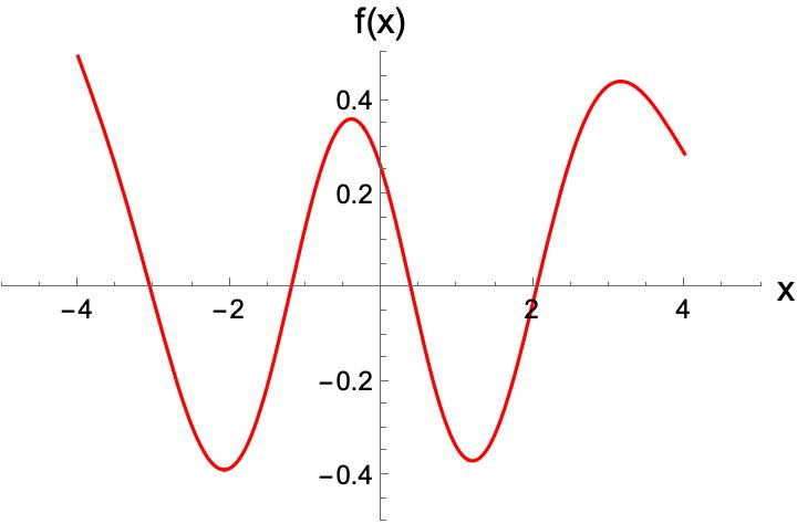
Figure 1: Plot of the parabolic cylinder function $f(x)={\rm D}_{3.5}(x)$ for $-4<x<4$; $f(x)$ is not a harmonic-oscillator eigenfunction because it blows up when $x$ is large and negative. Note that $f(x)$ has four real zeros.

The four real zeros of $f(x)$, as shown in Fig. 1, are located at

$$-3.04735...,\leavevmode\nobreak\ \leavevmode\nobreak\ -1.19090...,\leavevmode\nobreak\ \leavevmode\nobreak\ 0.39183...,\leavevmode\nobreak\ \leavevmode\nobreak\ 2.04542...\,.$$ (2)

There are no other zeros in the complex-$x$ plane.

One way to find these zeros in (2) is to (i) expand $f(x)$ in a Taylor series, (ii) truncate this series to obtain a polynomial, and (iii) find the roots of the polynomial. The $2N$-term Taylor series for ${\rm D}_{3.5}(x)$ has the form

$${\rm D}_{3.5}(x) = {\rm D}_{3.5}(0)\sum_{n=0}^{N-1}x^{2n}\frac{a_{n}}{(2n)!}$$ (3)

$$\quad+{\rm D}_{3.5}^{\prime}(0)\sum_{n=0}^{N-1}x^{2n+1}\frac{b_{n}}{(2n+1)!}.$$

For even powers of $x$, $a_{0}=1$, $a_{1}=-4$, and $a_{n}=-4a_{n-1}+\mbox{$\textstyle{\frac{1}{2}}$}(n-1)(2n-3)a_{n-2}$; for odd powers of $x$, $b_{0}=1$, $b_{1}=-4$, and $b_{n}=-4b_{n-1}+\mbox{$\textstyle{\frac{1}{2}}$}(n-1)(2n-1)b_{n-2}$.

The Taylor series (3) has an infinite radius of convergence but many terms are required to obtain accurate approximations to the zeros of ${\rm D}_{3.5}(x)$. In Fig. 2 we plot the zeros of the 9th-degree Taylor polynomial. A 17th-degree Taylor polynomial gives slightly better approximations to the zeros, as we see in Fig. 3. Figures 4 and 5 display the roots of 25th-degree and 33rd-degree Taylor polynomials. As expected, the real zeros continue to approach the exact zeros of the parabolic cylinder function and the spurious zeros continue to move slowly outward as the degree of the Taylor polynomial increases.

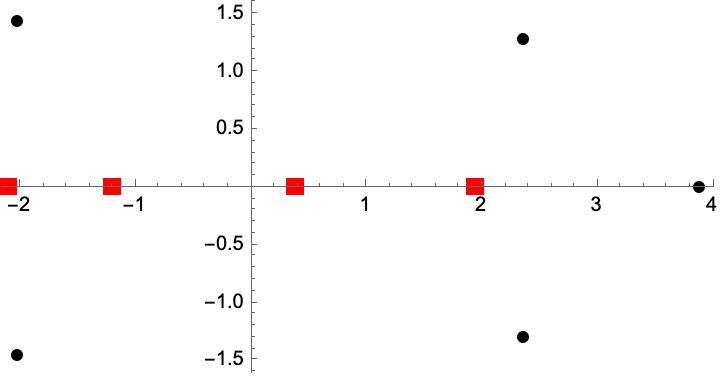
Figure 2: [color online] Roots of the 9th-degree Taylor-polynomial approximation to ${\rm D}_{3.5}(x)$ plotted in the complex-$x$ plane. Four real roots (red squares) are located at $x=-2.09226...$, $-1.19286...$, $0.39183...$, $1.94724...$, which are moderately close to the exact roots of $f(x)$ given in (2). The remaining roots (black dots) are spurious zeros that gradually move outward to complex $\infty$ as the degree of the Taylor polynomial increases.

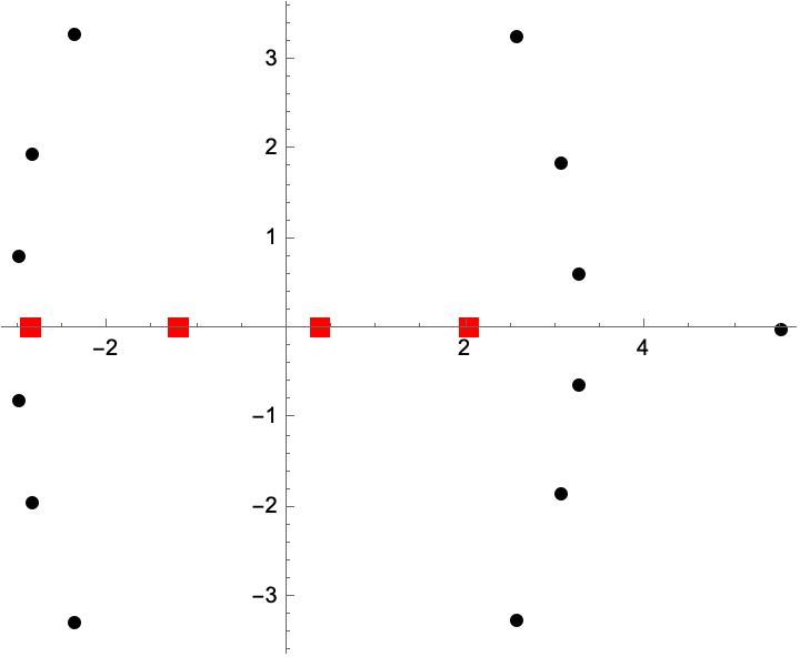
Figure 3: [color online] Roots of the 17th-degree Taylor polynomial approximation to ${\rm D}_{3.5}(x)$ plotted in the complex-$x$ plane. The real roots (red squares) lie at $x=-2.84103...$, $-1.19090...$, $0.39183...$, $2.04519...$ and are fairly close to their exact values in (2). Spurious roots (black dots) lie along parenthesis-shaped curves along with an isolated spurious root on the positive-real axis.

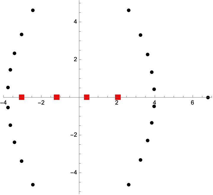
Figure 4: [color online] Roots of the 25th-degree Taylor polynomial approximation to ${\rm D}_{3.5}(x)$ plotted in the complex-$x$ plane. Real roots (red squares) at $x=-3.04510...$, $-1.19090...$, $0.39183...$, $2.04545...$ are closer to their exact values in (2). All but one of the spurious roots (black dots) lie on parenthesis-shaped curves that expand outward slowly as the degree of the Taylor polynomial increases. The isolated spurious root on the positive-real axis also moves outward.

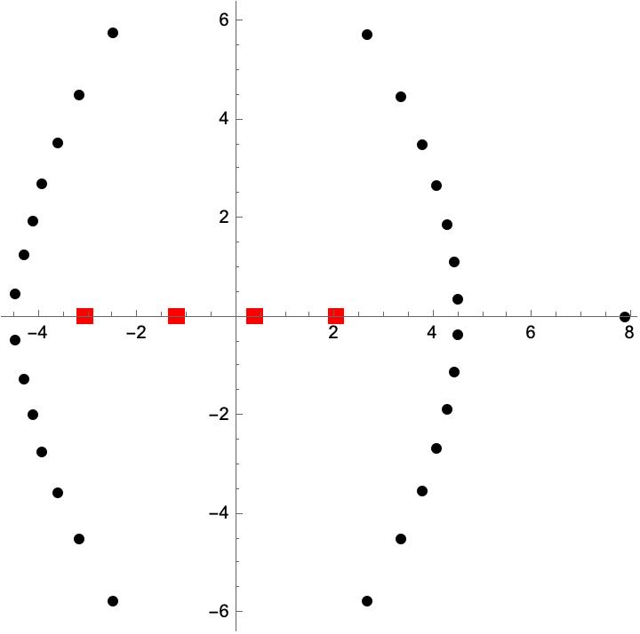
Figure 5: [color online] Roots of the 33rd-degree Taylor polynomial approximation to ${\rm D}_{3.5}(x)$ plotted in the complex-$x$ plane. Real roots (red squares) at $x=-3.04735...$, $-1.19090...$, $0.39183...$, $2.04542...$ are now are quite close to their exact values in (2). Spurious roots (black dots) lie on parenthesis-shaped curves and the isolated spurious root on the positive-real axis continue to move slowly outward.

Why is such a high-degree Taylor polynomial required to provide accurate approximations to the four zeros of the parabolic cylinder function? The answer is that, as shown in Fig. 1, the parabolic cylinder function behaves differently on the positive-real and the negative-real axes; it decays exponentially like $\exp\big{(}\!-\!\mbox{$\textstyle{\frac{1}{4}}$}x^{2}{\big{)}}$ on the positive-real axis but grows exponentially like $\exp\big{(}\mbox{$\textstyle{\frac{1}{4}}$}x^{2}\big{)}$ on the negative-real axis. However, as the Taylor series converges everywhere in the complex plane, it is difficult for the Taylor polynomials to provide accurate approximations on both the positive and the negative axes.

Asymptotic series do not suffer from this problem because such series are not valid in all directions in the complex plane. Their validity is limited to wedge-shaped regions called Stokes sectors. The asymptotic series representation for ${\rm D}_{3.5}(x)$ is

$${\rm D}_{3.5}(x) \sim e^{-x^{2}/4}\,x^{-7/2}\sum_{n=0}^{\infty}x^{-2n}\frac{c_{n}}{2^{n}n!}$$ (4)

$$\quad\big{(}|x|\to\infty,\leavevmode\nobreak\ -\mbox{$\textstyle{\frac{3}{4}}$}\pi<{\rm arg}\,x<\mbox{$\textstyle{\frac{3}{4}}$}\pi\big{)},$$

where $c_{n}=(-1)^{n}\Gamma\big{(}\frac{9}{2}\big{)}\Gamma\big{(}2n-\frac{9}{2}\big{)}/\pi$. This asymptotic series is valid in a Stokes sector of angular opening $270^{\circ}$ that includes the positive-real axis but not the negative-real axis. Thus, if we factor off the leading asymptotic behavior to obtain a polynomial, this polynomial will not give useful information about the negative zeros.

Although the asymptotic series is valid as $|x|\to\infty$, early terms provide good approximations to the positive zeros. The positive-real roots ($x=0.59521$ and $x=2.04530$) of the five-term polynomial ($1+\alpha x^{2}+\beta x^{4}+\gamma x^{6}+\delta x^{8}$) are already quite accurate (see Fig. 6); the second root is accurate to one part in 20,000.

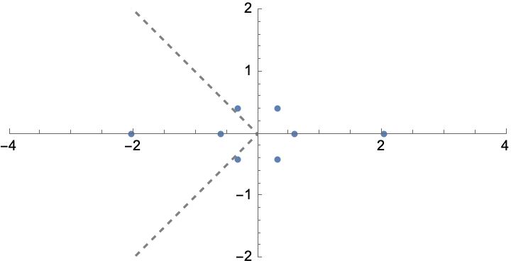
Figure 6: All eight roots of the five-term polynomial obtained from the truncated asymptotic expansion (4) plotted in the complex-$x$ plane. The two roots on the positive axis are numerically quite accurate. The other six roots are spurious. Dashed lines indicate the edges of the Stokes sector in which the asymptotic series is valid.

As the degree of the polynomial obtained from the asymptotic series increases, the ring of spurious zeros expands. For the ten-term polynomial this ring expands past the smaller of the two positive zeros, but there is still a very good approximation to the larger positive root (see Fig. 7). For the fifteen-term polynomial, this ring expands past the second positive zero and is no longer directly useful (see Fig. 8). Summation techniques such as Padé approximation give even better accuracy but we do not discuss this here.

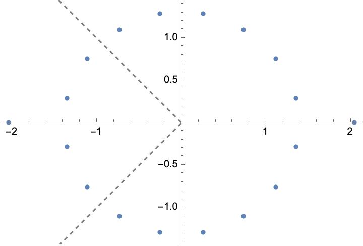
Figure 7: All eighteen roots of the ten-term polynomial obtained from the truncated asymptotic expansion (4). The roots are shown as dots in the complex-$x$ plane. Compared with Fig. 6, the ring of spurious roots has moved outward past the smaller positive zero of the parabolic cylinder function ${\rm D}_{3.5}(x)$ at $x=0.39183$ but the second positive zero is given accurately.

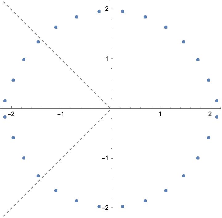
Figure 8: All 28 roots of the fifteen-term polynomial obtained from the truncated asymptotic expansion (4). The ring of spurious roots in the complex-$x$ plane has now expanded past the actual zeros of the parabolic cylinder function. Thus, without summation techniques the asymptotic series in (4) is no longer useful.

Without using summation techniques, the accuracy of an asymptotic-series approximation typically increases as we include more terms until it reaches an optimal level and then it decreases. This is illustrated in Fig. 9, which shows the value of the root of the asymptotic-series polynomial near 2 as a function of the number of terms in the polynomial. Note that the root oscillates about the exact zero of the parabolic cylinder function. Optimal accuracy is attained for the 6-term polynomial after which the accuracy decreases rapidly.

To summarize these findings, if we use a Taylor expansion to determine the roots of the parabolic cylinder function, we find more roots than the function actually has, and their number increases with the order of the expansion. Most of these spurious roots are imaginary but there is at least one real spurious root. To distinguish between actual and spurious roots one can use the criterion of stability; that is, one can argue that the spurious roots move outward in the complex plane while the positions of the actual roots stabilize as the order of the expansion increases. Finally, the order of approximation that is required to obtain an accurate result is high, which is unfortunate. We emphasize that the coefficients of the Taylor expansion remain unchanged as we go to higher order. This is not the case for the polynomials associated with the DS equations.

The asymptotic series approach also has advantages and disadvantages. Its region of validity is limited to the interior of a Stokes sector and not the entire complex plane. Thus, the number of roots that it can possibly find is also limited. However, in its region of validity, the convergence is fast and requires only very few terms. Like the Taylor expansion, the asymptotic series also has many other roots in the complex plane that are spurious.

Evidently, without prior knowledge of a function, it may be difficult to determine from a polynomial expansion of that function which roots are close to the actual roots and which roots are spurious. In the following sections, we restrict our analysis to quantum field theories in $D=0$ because we can find analytic solutions. This allows us to investigate the systematics of finding the correct roots from the polynomial DS equations.

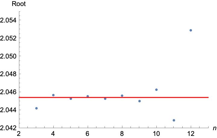
Figure 9: The root near $x=2$ of the polynomial obtained from the truncated asymptotic series approximation to the parabolic cylinder function plotted as a function of the degree of the polynomial. The six-term polynomial gives optimal accuracy after which the accuracy rapidly decreases.

III Derivation of DS Equations

The objective in quantum field theory is to calculate the Green’s functions $\gamma_{n}(x_{1},\,x_{2},\,...,\,x_{n})$, which are defined as vacuum-expectation values of time-ordered products of the field $\phi(x)$:

$$\gamma_{n}(x_{1},x_{2},...x_{n})\equiv\langle 0|{\rm T}\big{\{}\phi\big{(}x_{1}\big{)}\phi\big{(}x_{2}\big{)}...\phi\big{(}x_{n}\big{)}\big{\}}|0\rangle.$$

These Green’s functions are then combined into structures called cumulants that give the connected Green’s functions $G_{n}(x_{1},x_{2},...x_{n})$. The connected Green’s functions are correlation functions that contain the physical content (energy spectrum, scattering amplitudes) of the quantum field theory. In principle, the program is first to solve the field equations (which are partial differential equations like the classical equations of fluid mechanics) for the quantum field $\phi(x)$ and then to calculate the vacuum expectation values of products of the fields directly.

It is advantageous to calculate the connected Green’s functions $G_{n}$, rather than the nonconnected Green’s functions $\gamma_{n}$ because this eliminates the problem of vacuum divergences. As a consequence of translation invariance, each disconnected contribution to $\gamma_{n}$ introduces an additional factor of the spacetime volume $V$, which is an infinite quantity when $D>0$.

The difficulty in quantum field theory is that the field $\phi(x)$ is an operator-valued distribution rather than a function. Free fields obey linear differential equations but interacting fields obey nonlinear differential equations. (The field equation for a $g\phi^{4}$ quantum field theory contains a cubic term.) Unfortunately, products of fields are singular and require great care to define them properly.

An early approach to this difficulty was to calculate Green’s functions in terms of Feynman diagrams. This perturbative procedure (in powers of the coupling constant $g$) avoids high-level mathematical analysis and reduces the problem to the evaluation of integrals. Indeed, in the early days of quantum field theory one view was that one could simply define a field theory as nothing but a set of Feynman rules and thereby avoid technical mathematical problems R3 .

However, Feynman perturbation theory has its own mathematical difficulties: First, individual terms in the graphical expansion may be infinite and must be renormalized to remove the infinities. Second, the resulting renormalized perturbation series is divergent and may not be easily summable. Third, nonperturbative effects are difficult or even impossible to obtain by using perturbative graphical methods alone.

Dyson and Schwinger developed another technique for calculating the Green’s functions that requires only c-number functional analysis (differential and integral equations), so one need not be concerned about operators, Hilbert spaces, and other mathematical issues R4 ; R5 ; R6 . In principle, one can use this technique to obtain the nonperturbative as well as the perturbative behavior of Green’s functions. The procedure is to (i) construct an infinite system of coupled equations called Dyson-Schwinger (DS) equations that is satisfied exactly by the connected Green’s functions, and then (ii) truncate the infinite set of equations to a finite closed system of coupled equations that can be solved to provide approximations to the first few connected Green’s functions.

To be precise, the DS equations are an infinite triangular system of coupled equations obeyed by the connected Green’s functions $G_{n}$. Each new equation introduces additional Green’s functions so a truncation of the system always contains more Green’s functions than equations and the truncated system is underdetermined. An unbiased solution strategy is to close the truncated system by setting the highest Green’s function (or Green’s functions) to zero. The system can then be solved by successive elimination. The question investigated here is whether this procedure gives increasingly accurate approximations to the Green’s functions as the size of the truncated system increases. We also examine the differences between Hermitian and non-Hermitian theories. We will see below that the accuracy of a first-order calculation of $G_{2}$ is significantly higher for a one-dimensional Hermitian $\phi^{4}$ theory than for a non-Hermitian $\mathcal{PT}$-symmetric $-\phi^{4}$ theory.

The DS equations for a quantum field theory can be derived directly from the Euclidean functional integral

$$Z[J]=\int\!\mathcal{D}\phi\,\exp\bigg{[}\int\!dx\{-\mathcal{L}[\phi(x)]+J(x)\phi(x)\}\bigg{]},$$ (5)

where $\mathcal{L}$ is the Lagrangian and $J$ is a c-number external source. Here, $Z[0]$ is the Euclidean partition function and $\langle 0_{+}|0_{-}\rangle_{J}\equiv Z[J]$ represents the vacuum-persistence amplitude; that is, the probability amplitude for the ground state in the far past to remain in the ground state in the far future despite the action of the external source $J$.

The vacuum-persistence functional is a generating function for the Green’s functions. If we take $n$ functional derivatives of $Z[J]$ with respect to $J$ and then set $J\equiv 0$, we obtain the $n$-point Green’s function $\gamma_{n}$:

$$\gamma_{n}(x_{1},\,...\,x_{n})=\frac{\delta}{\delta J(x_{1})}...\frac{\delta}{\delta J(x_{n})}Z[J]\Big{|}_{J\equiv 0}.$$

And, if we take $n$ functional derivatives of $\log(Z[J])$ with respect to $J$ and set $J\equiv 0$, we obtain the connected $n$-point Green’s function:

$$G_{n}(x_{1},\,...\,x_{n})=\frac{\delta}{\delta J(x_{1})}...\frac{\delta}{\delta J(x_{n})}\log(Z[J])\big{|}_{J\equiv 0}.$$ (6)

III.1 Example: Hermitian quartic theory in $D=1$

For a Hermitian massless $\phi^{4}$ theory in one-dimensional spacetime, we begin with the Euclidean functional integral $Z[J]=\int D\phi e^{-\int dt\mathcal{L}}$, where

$$\mathcal{L}=\mbox{$\textstyle{\frac{1}{2}}$}{\dot{\phi}}^{2}+\mbox{$\textstyle{\frac{1}{4}}$}g\phi^{4}-J\phi\quad(g>0).$$ (7)

The field equation for this theory is $-{\ddot{\phi}}(t)+g\phi^{3}(t)-J(t)=0$. We take the vacuum expectation value of the field equation and divide by $Z[J]$:

$$-{\ddot{G}}_{1}(t)+g\gamma_{3}(t,t,t)/Z[J]=J(t),$$ (8)

where $G_{1}(t)$ and $\gamma_{3}(t,t,t)$ are functionals of $J$.

To obtain the DS equations for the connected Green’s functions we eliminate the nonconnected Green’s function $\gamma_{3}$ in (8) in favor of connected Green’s functions. We functionally differentiate the equation $\gamma_{1}(t)=\langle 0|\phi(t)|0\rangle=Z[J]G_{1}(t)$ repeatedly with respect to $J(t)$:

$$\gamma_{2}(t,t)=\langle 0|\phi^{2}(t)|0\rangle=Z[J]G_{2}(t,t)+Z[J]G_{1}^{2}(t),$$

$$\gamma_{3}(t,t,t) = \langle 0|\phi^{3}(t)|0\rangle$$

$$= Z[J]G_{3}(t,t,t)+3Z[J]G_{1}(t)G_{2}(t,t)$$

$$\quad+Z[J]G_{1}^{3}(t).$$

We then divide this equation by $Z[J]$ and use the result to eliminate $\gamma_{3}$ in (8):

$$-{\ddot{G}}_{1}(t)+g[G_{3}(t,t,t)+3G_{1}(t)G_{2}(t,t)$$

$$\qquad\qquad+G_{1}^{3}(t)]=J(t).$$ (9)

This is the key equation; the entire set of DS equations is obtained from (9) by repeated differentiation with respect to $J$ and setting $J\equiv 0$. To get the first DS equation we set $J\equiv 0$ in (9). This restores translation invariance, so $G_{1}$ is a constant and ${\ddot{G}}_{1}=0$. Parity invariance implies that all odd-numbered Green’s functions vanish. Thus, the first DS equation becomes trivial: $0=0$.

To get the second DS equation we functionally differentiate (9) once with respect to $J(s)$, set $J\equiv 0$, and drop all odd-numbered Green’s functions:

$$-{\ddot{G}}_{2}(s-t)+M^{2}G_{2}(s-t)+gG_{4}(s,t,t,t)=\delta(s-t),$$ (10)

where the renormalized mass is

$$M^{2}=3gG_{2}(0).$$ (11)

We cannot solve (10) because it is one equation in two unknowns, $G_{2}$ and $G_{4}$. As stated above, each new DS equation introduces one new unknown Green’s function: The third DS equation is trivial but the fourth contains $G_{6}$, the fifth is trivial but the sixth contains $G_{8}$, and so on. To proceed, we simply set $G_{4}=0$ in (10).

To solve the resulting equation we take a Fourier transform to get $(p^{2}+M^{2}){\tilde{G}}_{2}(p)=1$. Thus, the two-point connected Green’s function in momentum space is

$${\tilde{G}}_{2}(p)=1/\big{(}p^{2}+M^{2}\big{)}.$$

Taking the inverse transform, we get $G_{2}(t)=e^{-M|t|}/(2M)$, so $G_{2}(0)=1/(2M)$. Inserting $G_{2}(0)$ into (11) gives a cubic equation for the renormalized mass whose solution for $g=1$ is $M=(3/2)^{1/3}=1.145...\,$.

To check the accuracy of this result we note that the renormalized mass is the energy of the lowest excitation above the ground state. For this model (massless quantum anharmonic oscillator) the exact answer is $M=E_{1}-E_{0}=1.088...\,$. Thus, the DS result is 5.2% high, which is not bad for a leading-order truncation.

III.2 Example: $\mathcal{PT}$-symmetric quartic theory in $D=1$

We obtain a non-Hermitian $\mathcal{PT}$-symmetric massless $\phi^{4}$ theory in $D=1$ if $g$ in (7) is negative. In this case the Green’s functions are not parity symmetric, so the odd-$n$ Green’s functions do not vanish. The first DS equation is not trivial, $3G_{2}(0)+G_{1}^{2}=0$, where we have divided by the common factor $G_{1}$. Following the procedure in the example above, the second DS equation leads to two more equations

$$M^{2}=3g[G_{1}^{2}+G_{2}(0)],\quad G_{2}(0)=1/(2M).$$

We set $g=-1$ and solve the three equations above for the renormalized mass:

$$M=3^{1/3}=1.442...\,.$$ (12)

The exact value of $M$ obtained by solving the Schrödinger equation for the $\mathcal{PT}$-symmetric quantum-mechanical Hamiltonian $H=\mbox{$\textstyle{\frac{1}{2}}$}p^{2}-\mbox{$\textstyle{\frac{1}{4}}$}x^{4}$ is $M=E_{1}-E_{0}=1.796...\,$. Thus, the result in (12) is 19.7% low.

The two examples above raise the following question: Does the accuracy improve if we perform higher-level truncations of the DS equations? In general, this is not an easy question to answer because higher-order truncations of the DS equations lead to nonlinear integral equations, which require detailed numerical analysis. However, we can solve the DS equations in very high order to study the convergence in zero spacetime dimensions. In the next sections we examine this question in detail for the $D=0$ Hermitian $g\phi^{4}$ ($g>0$) theory, the $D=0$ non-Hermitian $i\phi^{3}$ theory, the $D=0$ non-Hermitian $g\phi^{4}$ ($g<0$) theory, the $D=0$ non-Hermitian $-i\phi^{5}$ theory, and the $D=0$ Hermitian $\phi^{6}$ theory.

IV $D=0$ Hermitian quartic theory

In zero-dimensional spacetime the functional integral (5) becomes the ordinary integral

$$Z[J]=\int_{-\infty}^{\infty}d\phi\,e^{-\mathcal{L}(\phi)},$$ (13)

where $\mathcal{L}(\phi)=\mbox{$\textstyle{\frac{1}{4}}$}\phi^{4}-J\phi$ and we have set $g=1$. The connected two-point Green’s function is an ordinary integral, which we evaluate exactly:

$$G_{2} = \int_{-\infty}^{\infty}d\phi\,\phi^{2}e^{-\phi^{4}/4}\Big{/}\int_{-\infty}^{\infty}d\phi\,e^{-\phi^{4}/4}$$ (14)

$$= 2\Gamma\big{(}\mbox{$\textstyle{\frac{3}{4}}$}\big{)}\big{/}\Gamma\big{(}\mbox{$\textstyle{\frac{1}{4}}$}\big{)}=0.675\,978...\,.$$

The theory defined in (13) has parity invariance when $J=0$, so all odd Green’s functions vanish, $G_{1}=G_{3}=G_{5}=\,...\,=0$ and the first nontrivial DS equation is $G_{4}=-3G_{2}^{2}+1$. If we truncate this equation by setting $G_{4}=0$ and solve the resulting equation $3G_{2}^{2}=1$, we get the approximate numerical result $G_{2}=1/\sqrt{3}=0.577\,350...\,$. In comparison with (14) this result is 14.6% low.

Let us include more DS equations: The first four are

$$G_{4}\! = \!-3G_{2}^{2}+1,$$

$$G_{6}\! = \!-12G_{2}G_{4}-6G_{2}^{3},$$

$$G_{8}\! = \!-18G_{2}G_{6}-30G_{4}^{2}-60G_{2}^{2}G_{4},$$

$$G_{10}\! = \!-24G_{2}G_{8}-168G_{4}G_{6}-126G_{2}^{2}G_{6}-420G_{2}G_{4}^{2},$$

and the next six are

$$G_{12}\! = \!-30G_{2}G_{10}-360G_{4}G_{8}-216G_{2}^{2}G_{8}-378G_{6}^{2}$$

$$\!-3024G_{2}G_{4}G_{6},$$

$$G_{14}\! = \!-36G_{2}G_{12}-660G_{4}G_{10}-330G_{2}^{2}G_{10}$$

$$\!-2376G_{6}G_{8}-7920G_{2}G_{4}G_{8}-8316G_{2}G_{6}^{2}$$

$$\!-41580G_{3}G_{5}G_{6}-27720G_{4}^{2}G_{6},$$

$$G_{16}\! = \!-42G_{2}G_{14}-1092G_{4}G_{12}-468G_{2}^{2}G_{12}$$

$$\!-6006G_{6}G_{10}-17160G_{2}G_{4}G_{10}-5148G_{8}^{2}$$

$$\!-61776G_{2}G_{6}G_{8}-102960G_{4}^{2}G_{8}-216216G_{4}G_{6}^{2},$$

$$G_{18}\! = \!-48G_{2}G_{16}-1680G_{4}G_{14}-630G_{2}^{2}G_{14}$$

$$\!-13104G_{6}G_{12}-32760G_{2}G_{4}G_{12}-34320G_{8}G_{10}$$

$$\!-180180G_{2}G_{6}G_{10}-300300G_{4}^{2}G_{10}$$

$$\!-154440G_{2}G_{8}^{2}-2162160G_{4}G_{6}G_{8}-756756G_{6}^{3},$$

$$G_{20}\! = \!-54G_{2}G_{18}-2448G_{4}G_{16}-816G_{2}^{2}G_{16}$$

$$\!-25704G_{6}G_{14}-57120G_{2}G_{4}G_{14}-95472G_{8}G_{12}$$

$$\!-445536G_{2}G_{6}G_{12}-742560G_{4}^{2}G_{12}-72930G_{10}^{2}$$

$$\!-7001280G_{4}G_{8}^{2}-1166880G_{2}G_{8}G_{10}$$

$$\!-8168160G_{4}G_{6}G_{10}-14702688G_{6}^{2}G_{8}$$

$$\!-17153136G_{6}G_{7}^{2},$$

$$G_{22}\! = \!-60G_{2}G_{20}-3420G_{4}G_{18}-1026G_{2}^{2}G_{18}$$ (15)

$$\!-46512G_{6}G_{16}-93024G_{2}G_{4}G_{16}$$

$$\!-232560G_{8}G_{14}-976752G_{2}G_{6}G_{14}$$

$$\!-1627920G_{4}^{2}G_{14}-503880G_{10}G_{12}$$

$$\!-3627936G_{2}G_{8}G_{12}-25395552G_{4}G_{6}G_{12}$$

$$\!-2771340G_{2}G_{10}^{2}-66512160G_{4}G_{8}G_{10}$$

$$\!-69837768G_{6}^{2}G_{10}-119721888G_{6}G_{8}^{2}.$$

Because the DS equations (15) are exact, we can find the precise values of all $G_{2n}$ sequentially by substituting the exact value of $G_{2}$ from (14) into (15). The results are given in Table 1. Observe that the $G_{2n}$ alternate in sign as $n$ increases, a feature that is not immediately evident from the structure of the equations in (15). Close examination of the terms contributing to a given $G_{2n}$ reveals that all terms are of similar size, so it is not easy to identify a dominant contribution.

The oscillation in sign of $G_{2n}$ as $n$ increases differs from the behavior of the disconnected Green’s functions,

$$\gamma_{2n}=\int_{-\infty}^{\infty}d\phi\phi^{2n}e^{-\phi^{4}/4}=2^{n-1/2}\Gamma(\tfrac{2n+1}{4}),$$ (16)

all of which from (16) are positive. The first eleven numerical values are also given in Table 1.

Table 1: Exact values of the first 11 nonzero connected Green’s functions (left) and the first 11 nonzero disconnected Green’s functions (right) for the Hermitian quartic theory (13).

$G_{2}^{\rm exact}$	$0.675\,978\,24$
$G_{4}^{\rm exact}$	$-0.370\,839\,74$
$G_{6}^{\rm exact}$	$1.154\,839\,49$
$G_{8}^{\rm exact}$	$-8.010\,060\,86$
$G_{10}^{\rm exact}$	$96.364\,571\,49$
$G_{12}^{\rm exact}$	$-1,775.987\,088\,64$
$G_{14}^{\rm exact}$	$46,449.956\,507\,74$
$G_{16}^{\rm exact}$	$-1,635,683.384\,912\,06$
$G_{18}^{\rm exact}$	$74,607,360.536\,889\,26$
$G_{20}^{\rm exact}$	$-4,278,841,318.741\,397\,69$
$G_{22}^{\rm exact}$	$301,366,607,264.871\,591\,99$

$\gamma_{2}^{\rm exact}$	$1.733$
$\gamma_{4}^{\rm exact}$	$2.56369$
$\gamma_{6}^{\rm exact}$	$5.199$
$\gamma_{8}^{\rm exact}$	$12.8185$
$\gamma_{10}^{\rm exact}$	$36.393$
$\gamma_{12}^{\rm exact}$	$115.366$
$\gamma_{14}^{\rm exact}$	$400.323$
$\gamma_{16}^{\rm exact}$	$1\,499.76$
$\gamma_{18}^{\rm exact}$	$6\,004.85$
$\gamma_{20}^{\rm exact}$	$25\,495.9$
$\gamma_{22}^{\rm exact}$	$114\,092.$

It is possible to check the expressions for the connected Green’s functions in (15) using an alternative, independent method. We calculate the $G_{2n}$ directly from a generating function $w(x)$, which in this case is possible, since we know $\gamma_{2n}$ explicitly: we can write down the generating function for $G_{2n}$ in terms of it,

$$w(x)=\ln\big{[}1+\frac{1}{2!}\frac{\gamma_{2}}{\gamma_{0}}x^{2}+\frac{1}{4!}\frac{\gamma_{4}}{\gamma_{0}}x^{4}+\frac{1}{6!}\frac{\gamma_{6}}{\gamma_{0}}x^{6}+\dots\big{]},$$ (17)

expand this in a Taylor series, and identify the $G_{2n}$ as $(2n!)\times$ the coefficient of $x^{2n}$. One easily finds that the coefficient of $x^{2}$ is $\Gamma(\tfrac{3}{4})/\Gamma(\tfrac{1}{4})$, so that one recovers the value of $G_{2}$ given in (14). The next five Green’s functions calculated in this way are

$$G_{4} = 1-12\frac{\Gamma(\tfrac{3}{4})^{2}}{\Gamma(\tfrac{1}{4})^{2}},$$

$$G_{6} = -24\frac{\Gamma(\tfrac{3}{4})}{\Gamma(\tfrac{1}{4})}+240\frac{\Gamma(\tfrac{3}{4})^{3}}{\Gamma(\tfrac{1}{4})^{3}},$$

$$G_{8} = -30+1\,344\frac{\Gamma(\tfrac{3}{4})^{2}}{\Gamma(\tfrac{1}{4})^{2}}-10\,080\frac{\Gamma(\tfrac{3}{4})^{4}}{\Gamma(\tfrac{1}{4})^{4}},$$

$$G_{10} = 4\,632\frac{\Gamma(\tfrac{3}{4})}{\Gamma(\tfrac{1}{4})}-120\,960\frac{\Gamma(\tfrac{3}{4})^{3}}{\Gamma(\tfrac{1}{4})^{3}}+725\,760\frac{\Gamma(\tfrac{3}{4})^{5}}{\Gamma(\tfrac{1}{4})^{5}}.$$

$$G_{12} = 9\,120-877\,536\frac{\Gamma(\tfrac{3}{4})^{2}}{\Gamma(\tfrac{1}{4})^{2}}+15\,966\,720\frac{\Gamma(\tfrac{3}{4})^{4}}{\Gamma(\tfrac{1}{4})^{4}}$$ (18)

$$\quad-79\,833\,600\frac{\Gamma(\tfrac{3}{4})^{6}}{\Gamma(\tfrac{1}{4})^{6}},$$

with the expansion of the logarithm leading to alternating signs of the terms contributing to each $G_{2n}$.

A numerical evaluation of (18) confirms the exact values given in Table 1. The analytic relationships among the $G_{2n}$, as derived from the DS equations (15), can be easily confirmed. This calculation confirms the DS equations, but (18) does not lend itself to an asymptotic analysis because the sign of $G_{2n}$ as evaluated from these expressions is determined by a delicate cancellation of terms having different signs. The alternation in signs of the $G_{2n}$ occurs because these functions are cumulants, reflecting only connected terms and therefore requiring subtractions. From the DS equations (15) it is not at all obvious that the signs are oscillating.

IV.1 Approximate solutions

As a rule, we do not know the exact solutions to the DS equations, and must therefore employ approximate methods of solution. The system of DS equations (15) is not closed. Rather it is triangular, and the number of unknowns is always one more than the number of equations. A standard unbiased procedure is to define a truncation scheme in which as a first approximation $G_{4}=G_{6}=G_{8}=...=0$; the next level of approximation is reached by setting $G_{6}=G_{8}=G_{10}=...=0$, the next by setting $G_{8}=G_{10}=G_{12}=G_{14}=...=0$, and so on.

To do this efficiently, we reorganize (15). We eliminate $G_{4}$ by substituting the first equation into the second, we eliminate $G_{6}$ by substituting the first two equations into the third, and so on. Continuing this way, we obtain an expression for $G_{2n}$ as an $n$th degree polynomial in $G_{2}$ only. We denote the monic form of these polynomials (where the highest power of $x$ is 1) as $P_{n}(G_{2})$. The first ten such polynomials are

$$P_{2}(x) = x^{2}-\tfrac{1}{3},$$

$$P_{3}(x) = x^{3}-\tfrac{2}{5}x,$$

$$P_{4}(x) = x^{4}-\tfrac{8}{15}x^{2}+\tfrac{1}{21},$$

$$P_{5}(x) = x^{5}-\tfrac{2}{3}x^{3}+\tfrac{193}{1890}x$$

$$P_{6}(x) = x^{6}-\tfrac{4}{5}x^{4}+\tfrac{277}{1575}x^{2}-\tfrac{76}{10395},$$

$$P_{7}(x) = x^{7}-\tfrac{14}{15}x^{5}+\tfrac{361}{1350}x^{3}-\tfrac{85}{3861}x,$$

$$P_{8}(x) = x^{8}-\tfrac{16}{15}x^{6}+\tfrac{356}{945}x^{4}-\tfrac{475792}{10135125}x^{2}+\tfrac{1229}{1091475},$$

$$P_{9}(x) = x^{9}-\tfrac{6}{5}x^{7}+\tfrac{529}{1050}x^{5}-\tfrac{13583}{160875}x^{3}$$

$$\quad+\tfrac{8413529}{1929727800}x,$$

$$P_{10}(x) = x^{10}-\tfrac{4}{3}x^{8}+\tfrac{613}{945}x^{6}-\tfrac{92464}{675675}x^{4}$$

$$\quad+\tfrac{3658792}{328930875}x^{2}-\tfrac{32372}{186642225},$$

$$P_{11}(x) = x^{11}-\tfrac{22}{15}x^{9}+\tfrac{7667}{9450}x^{7}-\tfrac{190319}{921375}x^{5}$$ (19)

$$\quad+\tfrac{130461193}{5638815000}x^{3}-\tfrac{61559809}{74996239500}x.$$

Truncating the DS equations (15) is equivalent to finding the zeros of these polynomials. We list the nonnegative zeros below (negative zeros are excluded because $G_{2}=M^{-2}$, where $M$ is the renormalized mass). The first seven sets of zeros are

$${\rm zero\leavevmode\nobreak\ of}\leavevmode\nobreak\ P_{2}: \leavevmode\nobreak\ 0.577350,$$

$${\rm zeros\leavevmode\nobreak\ of}\leavevmode\nobreak\ P_{3}: \leavevmode\nobreak\ 0.0,\leavevmode\nobreak\ \leavevmode\nobreak\ 0.632456,$$

$${\rm zeros\leavevmode\nobreak\ of}\leavevmode\nobreak\ P_{4}: \leavevmode\nobreak\ 0.336742,\leavevmode\nobreak\ \leavevmode\nobreak\ 0.648026,$$

$${\rm zeros\leavevmode\nobreak\ of}\leavevmode\nobreak\ P_{5}: \leavevmode\nobreak\ 0.0,\leavevmode\nobreak\ \leavevmode\nobreak\ 0.488357,\leavevmode\nobreak\ \leavevmode\nobreak\ 0.654350,$$

$${\rm zeros\leavevmode\nobreak\ of}\leavevmode\nobreak\ P_{6}: \leavevmode\nobreak\ 0.232147,\leavevmode\nobreak\ \leavevmode\nobreak\ 0.560220,\leavevmode\nobreak\ \leavevmode\nobreak\ 0.657466,$$

$${\rm zeros\leavevmode\nobreak\ of}\leavevmode\nobreak\ P_{7}: \leavevmode\nobreak\ 0.0,\leavevmode\nobreak\ \leavevmode\nobreak\ 0.376821,\leavevmode\nobreak\ \leavevmode\nobreak\ 0.597310,\leavevmode\nobreak\ \leavevmode\nobreak\ 0.659212,$$

$${\rm zeros\leavevmode\nobreak\ of}\leavevmode\nobreak\ P_{8}: \leavevmode\nobreak\ 0.176270,\leavevmode\nobreak\ \leavevmode\nobreak\ 0.466447,\leavevmode\nobreak\ \leavevmode\nobreak\ 0.618098,$$

$$\quad\leavevmode\nobreak\ \leavevmode\nobreak\ 0.660287,$$

and the next three sets of zeros are

$${\rm zeros\leavevmode\nobreak\ of}\leavevmode\nobreak\ P_{9}: \leavevmode\nobreak\ 0.0,\leavevmode\nobreak\ \leavevmode\nobreak\ 0.302770,\leavevmode\nobreak\ \leavevmode\nobreak\ 0.523189,\leavevmode\nobreak\ \leavevmode\nobreak\ 0.630624,$$

$$\quad\leavevmode\nobreak\ \leavevmode\nobreak\ 0.660997,$$

$${\rm zeros\leavevmode\nobreak\ of}\leavevmode\nobreak\ P_{10}: \leavevmode\nobreak\ 0.141830,\leavevmode\nobreak\ \leavevmode\nobreak\ 0.392352,\leavevmode\nobreak\ \leavevmode\nobreak\ 0.560204,$$

$$\quad\leavevmode\nobreak\ \leavevmode\nobreak\ 0.638652,\leavevmode\nobreak\ \leavevmode\nobreak\ 0.661493,$$

$${\rm zeros\leavevmode\nobreak\ of}\leavevmode\nobreak\ P_{11}: \leavevmode\nobreak\ 0.0,\leavevmode\nobreak\ \leavevmode\nobreak\ 0.251866,\leavevmode\nobreak\ \leavevmode\nobreak\ 0.456057,\leavevmode\nobreak\ \leavevmode\nobreak\ 0.585125,$$ (20)

$$\quad\leavevmode\nobreak\ \leavevmode\nobreak\ 0.644070,\leavevmode\nobreak\ \leavevmode\nobreak\ 0.661853.$$

The roots up to $n=80$ are plotted in Fig. 10. Note that all roots are real and nondegenerate, and range from 0 up to just below the exact value of $G_{2}$ in (14). If we did not already know the exact value $G_{2}$, we could not guess which root gives the best approximation to $G_{2}$. However, with increasing truncation order, the roots become more dense at the upper end of the range, so we would conjecture that the largest root gives the best approximation. Unfortunately, while the accuracy improves monotonically with the order of the truncation, it improves slowly; the largest root of $P(x)$ is still 1.85% below the exact value. Using Richardson extrapolation, we can determine the value to which the largest root converges R7 : $G_{2}=0.663\,488\dots$. Thus, the limiting value of the sequence of roots does not converge to the true value $G_{2}=0.675\,978\dots$ R1 . To understand this discrepancy, we examine the large-$n$ asymptotic behavior of the $G_{2n}$ in detail in the following subsection.

Figure 10: Zeros of $P_{n}(x)$ in (19) plotted as a function of $n$. The zeros are nondegenerate and range from 0 up to just below $0.675\,978...$, the exact value of $G_{2}$ in (14) (heavy horizontal line) and they become more dense at the upper end of this range. The zeros of successive polynomials interlace.

Figure 10 also shows that the zeros of successive polynomials $P_{n}(x)$ interlace. This interlacing behavior might suggest that the polynomials $P_{n}(x)$ form an orthogonal set with respect to some weight function, but this conjecture is false. Nevertheless, these polynomials do have interesting properties. In particular, there are relatively simple formulas for the polynomial coefficients: The coefficient of $x^{n}$, the highest power of $x$ in $P_{n}(x)$, is 1 (these are monic polynomials) and the formula for the coefficient of $x^{n-2}$, the second highest power of $x$, is $-\mbox{$\textstyle{\frac{2}{15}}$}n\leavevmode\nobreak\ \leavevmode\nobreak\ (n>2)$. The coefficient of $x^{n-4}$ is

$$\textstyle{\frac{1}{2!}}(\mbox{$\textstyle{\frac{2}{15}}$})^{2}[n^{2}-\textstyle{\frac{227}{84}}n]\quad(n>4),$$

the coefficient of $x^{n-6}$ is

$$-\textstyle{\frac{1}{3!}}(\mbox{$\textstyle{\frac{2}{15}}$})^{3}[n^{3}-\textstyle{\frac{227}{28}}n^{2}+\textstyle{\frac{31453}{2002}}n]\quad(n>6),$$

and the coefficient of $x^{n-8}$ is

$$\textstyle{\frac{1}{4!}}(\mbox{$\textstyle{\frac{2}{15}}$})^{4}[n^{4}-\textstyle{\frac{227}{14}}n^{3}+\textstyle{\frac{28505063}{336336}}n^{2}-\textstyle{\frac{404875283}{2858856}}n]\quad(n>8).$$

IV.2 Large-$n$ behavior of the Green’s functions $G_{2n}$

The question is whether it is valid to truncate the DS equations (15) by replacing $G_{2n}$ with zero. To answer this question we look at the asymptotic behavior of $G_{2n}$ for large $n$. We have shown both numerically and analytically R1 that the asymptotic behavior of $G_{2n}$ is

$$G_{2n}\sim 2r^{2n}(-1)^{n+1}(2n-1)!\quad(n\to\infty),$$ (21)

where $r=0.409\,505\,7...\,.$

To obtain this result analytically we substitute

$$G_{2n}=(-1)^{n+1}(2n-1)!\,g_{2n},$$

which is suggested by the numerical result in (21), and we define a generating function $u(x)$ for the numbers $g_{2n}$:

$$u(x)\equiv xg_{2}+x^{3}g_{4}+x^{5}g_{6}+...\,.$$ (22)

This generating function obeys the second-order nonlinear differential equation

$$u^{\prime\prime}(x)=3u^{\prime}(x)u(x)-u^{3}(x)-x,$$

subject to the initial conditions $u(0)=0$ and

$$u^{\prime}(0)=G_{2}=2\Gamma\big{(}\mbox{$\textstyle{\frac{3}{4}}$}\big{)}/\Gamma\big{(}\mbox{$\textstyle{\frac{1}{4}}$}\big{)}=0.675\,978\,240\,067\,285...\,.$$

The substitution $u(x)=-y^{\prime}(x)/y(x)$ then gives the third-order linear differential equation

$$y^{\prime\prime\prime}(x)=xy(x),$$

which is a higher-order generalization of the Airy equation $y^{\prime\prime}(x)=xy(x)$. The function $y(x)$ satisfies the initial conditions $y(0)=1$, $y^{\prime}(0)=0$, and

$$y^{\prime\prime}(0)=-G_{2}=-0.675\,978\,240\,067\,285...\,.$$

The exact solution $y(x)$ satisfying these boundary conditions is found by taking a cosine transform:

$$y(x)=\frac{2\sqrt{2}}{\Gamma(1/4)}\int_{0}^{\infty}dt\,\cos(xt)\,e^{-t^{4}/4}.$$ (23)

When $y(x)$ passes through 0, $u(x)$ becomes infinite, so the value of $x$ at which $y(x)=0$ determines the radius of convergence of the series (22) for the generating function. We find that $u(x)$ passes through 0 at $x=\pm 2.441\,968...\,$. Therefore, $r=1/x=0.409\,506...\,$, which confirms the numerical results in (21).

The asymptotic behavior in (21) is surprising; it shows that the connected Green’s functions $G_{2n}$ grow much faster with increasing $n$ than the nonconnected Green’s functions $\gamma_{2n}$ which are given exactly for all $n$ in (16). One might not expect $G_{2n}$ to grow faster than $\gamma_{2n}$ because we obtain the connected Green’s function by subtracting the disconnected parts from $\gamma_{2n}$. Surprisingly, subtracting disconnected parts makes the absolute values of the connected Green’s functions larger and not smaller with increasing $n$.

Even more remarkable is that neglecting the huge quantity $G_{2n}$ on the left side of the truncated DS equations (15) still leads to a reasonably accurate result for $G_{2}$, as Fig. 10 shows. This accuracy improves with increasing $n$. We can begin to understand this heuristically by observing that while the term on the left side is very big, the terms on the right side are of roughly comparable size because the coefficients are also big.

The numerical technique of Legendre interpolation provides a helpful analogy. Given a set of $n$ data points $x_{1},\,...,\,x_{n}$ at which we measure a function $f(x)$,

$$f(x_{1})=f_{1},\,...,\,f(x_{n})=f_{n},$$

Legendre interpolation fits this data by constructing a polynomial $P_{n-1}(x)$ of degree $n-1$ that passes exactly through the value $f(x_{k})$ at $x=x_{k}$ for all $1\leq k\leq n$. There is a simple formula for this polynomial. However, this construction has a serious problem; while the constructed polynomial passes exactly through the data points, between data points the polynomial exhibits wild oscillations where it becomes alternately large and positive and large and negative. This reveals a fundamental instability associated with high-degree polynomials. This instability is associated with the inherent stiffness of polynomials R8 . If there are many data points, it is much better to use a least-squares polynomial approximation, which passes close to, but not exactly through the input data points. (This explains why cubic splines are used to approximate functions rather than, say, octic splines.)

It is precisely the instability associated with the stiffness of high-degree polynomials that allows the DS approach to give reasonably accurate results! If we use the exact values of the Green’s functions on the right side of the DS equations (15), we obtain the exact value of the Green’s function on the left side, which is a huge number. However, changing the Green’s functions on the right side of (15) very slightly by replacing the exact values by the approximate values of the lower Green’s functions now gives 0, instead of $G_{2n}$.

Padé approximation does not improve the calculation of $G_{2}$ from the DS polynomials in (19). One might anticipate that Padé techniques would be useful because the coefficients of successive powers of $x$ alternate in sign. The approach would be to divide all odd-numbered polynomials by $x$ and then to replace $x^{2}$ in each polynomial by $y$. If one does this for $P_{11}$, for example, one can then calculate the $[1,4]$, $[2,3]$, $[3,2]$, and $[4,1]$ approximants. Unfortunately, the zeros of these approximants are not near the exact value of $G_{2}^{2}$, and such an attempt to improve the accuracy of the DS equations fails. Why does this approach fail? Padé approximation accelerates the convergence of a truncated series even if the series diverges. However, unlike the infinite Taylor series expansion of the parabolic cylinder function in (3) where the coefficients of powers of $x$ remain the same as the order is increased, the coefficients in the DS equations change from order to order. Other approaches, such as assuming a value of $G_{2n}$ estimated from $G_{2n-2}$ converge to a limit that is very slightly closer to the correct one, but which is still not correct, and thus also fail.

One approach does give excellent numerical results: If the left side of the DS equations is approximated by the asymptotic approximation (21), $G_{2}$ reaches an accuracy of seven decimal places in only six steps. (See Fig. 11.) At $n=7$, we have $G_{2}=0.675\,978\,218\ldots$ in comparison with the exact result $G_{2,\,{\rm exact}}=0.675\,978\,240\ldots\,.$

Figure 11: Results for $G_{2}$ plotted as a function of $n$ ($1\leq n\leq 30$) calculated using the asymptotic approximation for $G_{2n}$ in (21). We observe a dramatic improvement over Fig. 10; there is no longer a dense concentration of roots below the exact answer but rather an isolated root that is six orders of magnitude closer to the exact answer.

While we have gained six orders of magnitude in precision, the result in Fig. 11 is not exact. This is because (21) is only a leading-order asymptotic approximation. Higher-order asymptotic approximations for $G_{2n}$ will improve this impressive numerical result even further. This suggests that the DS equations can be used to provide extremely accurate solutions for the Green’s functions, even when $D>0$, but these equations must be supplemented by including the large-$n$ asymptotic behavior of the Green’s function $G_{2n}$. This asymptotic behavior cannot be determined from the DS equations; it must be obtained from a large-$n$ asymptotic approximation to the integral representing the Green’s function.

V $D=0$ non-Hermitian cubic theory

This section considers the cubic massless non-Hermitian $\mathcal{PT}$-symmetric Lagrangian

$$\mathcal{L}=\mbox{$\textstyle{\frac{1}{3}}$}ig\phi^{3}.$$ (24)

For (24) the connected one-point Green’s function is

$$G_{1}=\int dx\,x\exp(-ix^{3}/3)\Big{/}\int dx\,\exp(-ix^{3}/3),$$ (25)

where we take $g=1$. The path of integration lies inside a $\mathcal{PT}$-symmetric pair pair of Stokes sectors. These integrals can be evaluated exactly:

$$G_{1}=-i3^{1/3}\Gamma\big{(}\mbox{$\textstyle{\frac{2}{3}}$}\big{)}/\Gamma\big{(}\mbox{$\textstyle{\frac{1}{3}}$}\big{)}=-0.729\,011\,13...\,i.$$ (26)

The DS equations for the Lagrangian (24) are simpler than those in (15) for the Hermitian quartic theory. The first 19 DS equations are given by

$$G_{2}\! = \!-G_{1}^{2},$$

$$G_{3}\! = \!-2G_{1}G_{2}-i,$$

$$G_{4}\! = \!-2G_{2}^{2}-2G_{1}G_{3},$$

$$G_{5}\! = \!-6G_{2}G_{3}-2G_{1}G_{4},$$

$$G_{6}\! = \!-6G_{3}^{2}-8G_{2}G_{4}-2G_{1}G_{5},$$

$$G_{7}\! = \!-20G_{3}G_{4}-10G_{2}G_{5}-2G_{1}G_{6},$$

$$G_{8}\! = \!-20G_{4}^{2}-30G_{3}G_{5}-12G_{2}G_{6}-2G_{1}G_{7},$$

$$G_{9}\! = \!-70G_{4}G_{5}-42G_{3}G_{6}-14G_{2}G_{7}-2G_{1}G_{8},$$

$$G_{10}\! = \!-70G_{5}^{2}-112G_{4}G_{6}-56G_{3}G_{7}-16G_{2}G_{8}$$

$$\!-2G_{1}G_{9},$$

$$G_{11}\! = \!-252G_{5}G_{6}-168G_{4}G_{7}-72G_{3}G_{8}$$

$$\!-18G_{2}G_{9}-2G_{1}G_{10},$$

$$G_{12}\! = \!-252G_{6}^{2}-420G_{5}G_{7}-240G_{4}G_{8}$$

$$\!-90G_{3}G_{9}-20G_{2}G_{10}-2G_{1}G_{11},$$

$$G_{13}\! = \!-924G_{6}G_{7}-660G_{5}G_{8}-330G_{4}G_{9}-110G_{3}G_{10}$$

$$\!-22G_{2}G_{11}-2G_{1}G_{12},$$

$$G_{14}\! = \!-924G_{7}^{2}-1584G_{6}G_{8}-990G_{5}G_{9}-440G_{4}G_{10}$$

$$\!-132G_{3}G_{11}-24G_{2}G_{12}-2G_{1}G_{13},$$

$$G_{15}\! = \!-3432G_{7}G_{8}-2574G_{6}G_{9}-1430G_{5}G_{10}$$

$$\!-572G_{4}G_{11}-156G_{3}G_{12}-26G_{2}G_{13}-2G_{1}G_{14},$$

$$G_{16}\! = \!-3432G_{8}^{2}-6006G_{7}G_{9}-4004G_{6}G_{10}$$

$$\!-2002G_{5}G_{11}-728G_{4}G_{12}-182G_{3}G_{13}$$

$$\!-28G_{2}G_{14}-2G_{1}G_{15},$$

$$G_{17}\! = \!-12870G_{8}G_{9}-10010G_{7}G_{10}-6006G_{6}G_{11}$$

$$\!-2730G_{5}G_{12}-910G_{4}G_{13}$$

$$\!-210G_{3}G_{14}-30G_{2}G_{15}-2G_{1}G_{16},$$

$$G_{18}\! = \!-12870G_{9}^{2}-22880G_{8}G_{10}-16016G_{7}G_{11}$$

$$\!-8736G_{6}G_{12}-3640G_{5}G_{13}-1120G_{4}G_{14}$$

$$\!-240G_{3}G_{15}-32G_{2}G_{16}-2G_{1}G_{17},$$

$$G_{19}\! = \!-48620G_{9}G_{10}-38896G_{8}G_{11}-24752G_{7}G_{12}$$

$$\!-12376G_{6}G_{13}-4760G_{5}G_{14}-1360G_{4}G_{15}$$

$$\!-272G_{3}G_{16}-34G_{2}G_{17}-2G_{1}G_{18},$$

$$G_{20}\! = \!-48620G_{10}^{2}-87516G_{9}G_{11}-63648G_{8}G_{12}$$

$$\!-37128G_{7}G_{13}-17136G_{6}G_{14}-6120G_{5}G_{15}$$

$$\!-1632G_{4}G_{16}-306G_{3}G_{17}-36G_{2}G_{18}-2G_{1}G_{19}.$$

The coefficients in these equations can be checked easily; the sum of the coefficients on the right side of each equation is an increasing power of 2. For example, for $G_{8}$ the sum of the coefficients is $20+30+12+2=2^{6}$, and for $G_{9}$ the sum is $70+42+14+2=2^{7}$.

As in Sec. IV, we again use the unbiased truncation scheme of setting higher-order Green’s functions to zero. We obtain the leading approximation to $G_{1}$ by substituting the first of these equations into the second and truncating by setting $G_{3}=G_{4}=\dots=0$. The resulting cubic equation $G_{1}^{3}=\mbox{$\textstyle{\frac{1}{2}}$}i$ has three solutions, and we choose the solution that is consistent with $\mathcal{PT}$ symmetry:

$$G_{1}=-2^{-1/3}i=-0.793\,700\,53...\,i.$$ (28)

This result differs by $8.9\%$ from the exact value of $G_{1}$ in (26). However, the accuracy improves if we include more DS equations: We close the system by using the first equation to eliminate $G_{2}$, the second to eliminate $G_{3}$, and so on. The result is that the right side of the $G_{n}$ equation becomes a polynomial of degree $n$ in the variable $G_{1}$, and we truncate the system by setting the left side to zero and finding the roots of this polynomial.

At first, the roots consistent with $\mathcal{PT}$ symmetry that are obtained with this procedure seem to approach the exact value of $G_{1}$ in (26) but unlike the roots for the Hermitian quartic theory, where the approach is monotone (see Fig. 10), the approach here is oscillatory at first: For the $n=4$ truncation the closest root is $-0.693\,361\,27...\,i$, which is smaller in magnitude than the exact value of $G_{1}$, and for $n=5$ the closest root is $-0.746\,900\,79...\,i$, which is larger in magnitude than the exact value. This pattern seems to persist: For $n=6$ the closest root is $-0.712\,564\,55...\,i$ and for $n=7$ the closest root is $-0.739\,871\,08...\,i$. However, for $n=8$ this pattern breaks: The closest root is $-0.712\,368\,70...\,i$, which is smaller in magnitude than the exact value, but is a slightly worse approximation than the $n=6$ root.

The departure from the oscillatory convergence pattern at $n=8$ signals a new behavior. The closest root for $n=9$ is $G_{1}=-0.738\,595\,46...\,i$, which is slightly better than the $n=7$ root, but for $n=10$ we observe a qualitative change in the character of the approximants. The polynomial associated with $G_{10}$ is

$$G_{10}=40\big{(}9072G_{1}^{10}-7560iG_{1}^{7}-1881G_{1}^{4}+119iG_{1}\big{)}.$$

If we truncate by setting the right side to zero and ignore the trivial root at 0, we see that all nontrivial roots come in triplets located at the vertices of equilateral triangles. The roots that are closest to the exact value of $G_{1}$, which lies on the negative-imaginary axis, are not pure imaginary. Rather, there is a pair of roots close to and on either side of the negative-imaginary axis at $-0.717\,367\,67...\,i\pm 0.016\,050\,677...\,.$

For higher truncations we find an accumulation of roots near the exact negative-imaginary value in (26), but arranged in a ring around this exact value. We have solved the DS equations up to the 200th truncation and we plot the solutions as dots in the complex plane in Fig. 12.

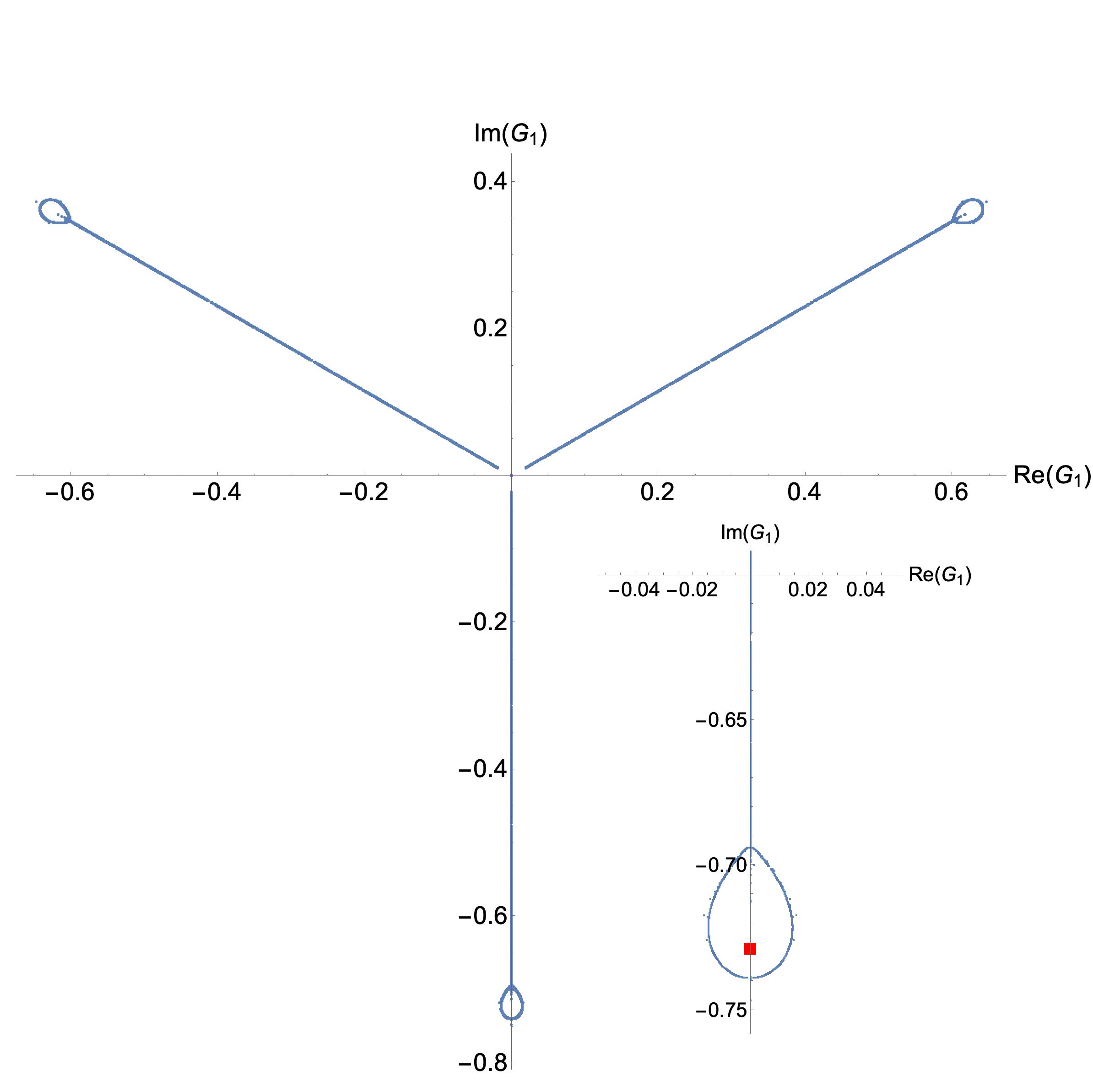
Figure 12: All solutions $G_{1}$ to the DS equations from the third to the 200th truncation plotted in the complex plane. The exact value of $G_{1}$ is $-0.72901113...\,i$. The full set of solutions has threefold symmetry; solutions lie on a three-bladed propeller with each blade having a small dense loop of solutions at the end. The inset shows that the exact solution (red square) lies on the negative-imaginary axis inside this loop.

We seek solutions that are near the negative-imaginary axis for two reasons: First, $\mathcal{PT}$ symmetry requires that $G_{1}$ be negative imaginary. Second, the first equation in (V), $G_{2}=-G_{1}^{2}$, shows that otherwise $G_{2}$ will not be positive; the second Green’s function must be positive because $G_{2}=M^{-2}$, where $M$ is the renormalized mass. A blow-up of the ring structure on the negative-imaginary axis is shown in Fig. 13 for the solution to the $n=200$ polynomial only. This emphasizes that the roots on the ring are not approaching the exact value of $G_{1}$ shown in Fig. 12 as $n$ increases, but rather are just becoming dense on the ring.

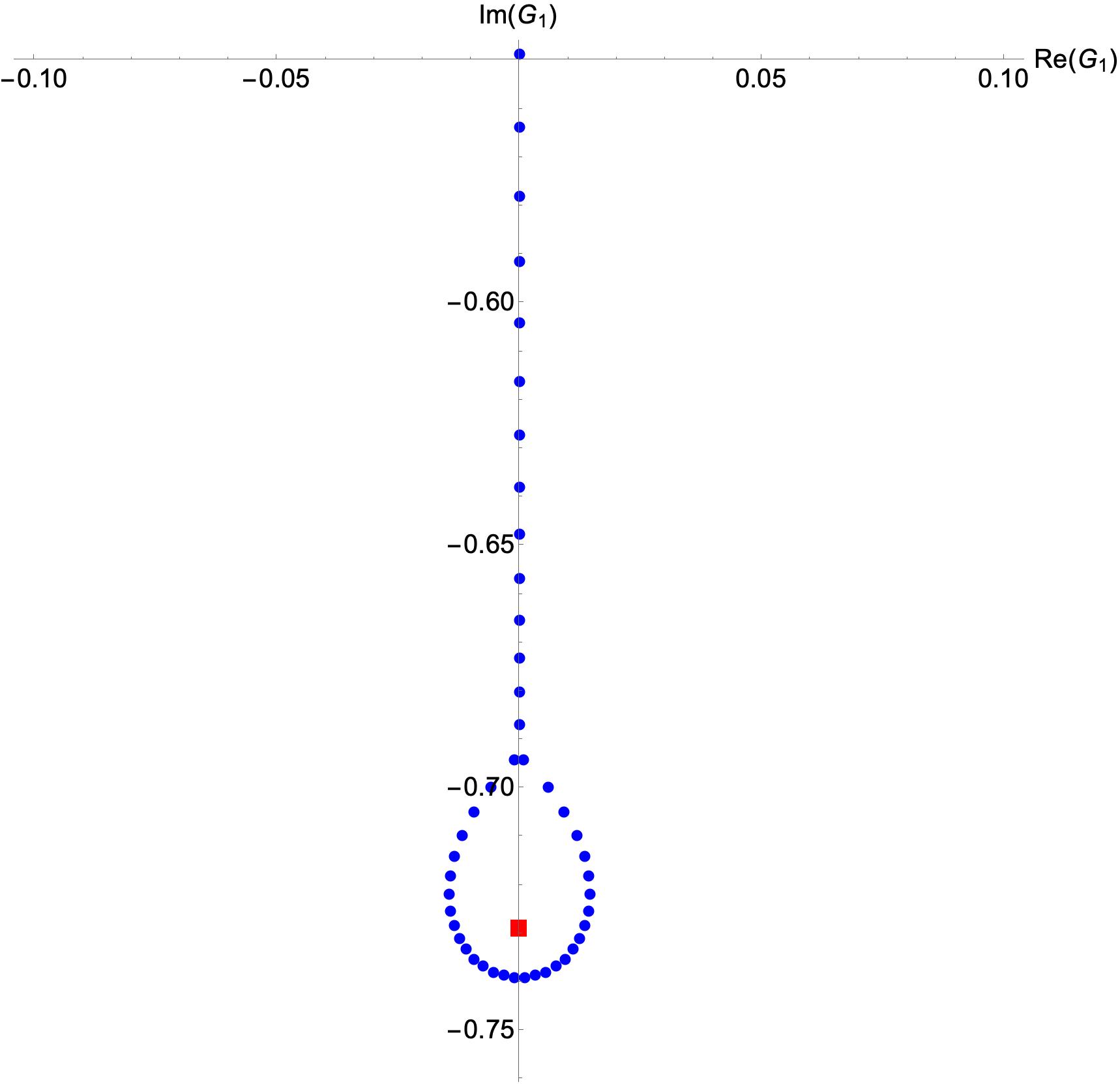
Figure 13: [color online] Blowup of the negative imaginary axis for the solution $n=200$ showing the loop-shaped concentration of solutions for $G_{1}$ around the exact value of $G_{1}$, which lies in the interior of the loop as shown in Fig. 12.

The three-fold symmetry of the roots in Fig. 12 arises because the monic polynomial equations that come from solving successively truncated DS equations contain only powers of $x^{3}$ (after we exclude the trivial roots at 0):

$$P_{3n}(x)=x^{3n}+C_{1}x^{3n-3}+C_{2}x^{3n-6}+...+C_{n}.$$ (29)

Five such polynomials (with factors of $i$ excluded) are

$$P_{3} = x^{3}+\tfrac{1}{2},$$

$$P_{6} = x^{6}+\tfrac{1}{2}x^{3}+\tfrac{1}{20},$$

$$P_{9} = x^{9}+\tfrac{3}{4}x^{6}+\tfrac{87}{560}x^{3}+\tfrac{1}{160},$$ (30)

$$P_{12} = x^{12}+x^{9}+\tfrac{93}{280}x^{6}+\tfrac{13}{336}x^{3}+\tfrac{7}{8800},$$

$$P_{15} = x^{15}+\tfrac{5}{4}x^{12}+\tfrac{4}{7}x^{9}+\tfrac{19}{168}x^{6}+\tfrac{56909}{6726720}x^{3}+\tfrac{1}{9856}.$$

Like the coefficients of the polynomials in (19), the coefficients $C_{k}$ in (29) have a fairly simple structure:

$$C_{1}(n) = \tfrac{1}{1!}\big{(}\mbox{$\textstyle{\frac{1}{4}}$}\big{)}^{1}n\quad(n>1),$$

$$C_{2}(n) = \tfrac{1}{2!}\big{(}\mbox{$\textstyle{\frac{1}{4}}$}\big{)}^{2}\big{(}n^{2}-\tfrac{47}{35}n\big{)}\quad(n>2),$$

$$C_{3}(n) = \tfrac{1}{3!}\big{(}\mbox{$\textstyle{\frac{1}{4}}$}\big{)}^{3}\big{(}n^{3}-\tfrac{47\cdot 3}{35}n^{2}+\tfrac{134}{35}n\big{)}\quad(n>3),$$

$$C_{4}(n) = \tfrac{1}{4!}\big{(}\mbox{$\textstyle{\frac{1}{4}}$}\big{)}^{4}\big{(}n^{4}-\tfrac{47\cdot 6}{35}n^{3}+\tfrac{25387}{1225}n^{2}-\tfrac{1471121}{175175}n\big{)}\^{A}~$$ (31)

$$\qquad(n>4).$$

V.1 Asymptotic behavior of $G_{n}$ for large $n$

In Sec. IV we investigated the large-$n$ asymptotic behavior of the Green’s functions in order to study the validity of the truncation procedure for the quartic Hermitian theory. We repeat this analysis for the non-Hermitian cubic theory. The DS equations (26) and (V) determine the exact values of the $G_{n}$. These are listed in Table 2.

Table 2: Exact values of the first 14 nonzero connected Green’s functions for the $\mathcal{PT}$-symmetric cubic theory.

$G_{2}^{\rm exact}=0.531\,457\,23$	$G_{3}^{\rm exact}=-0.225\,123\,53\,i$
$G_{4}^{\rm exact}=-0.236\,658\,45$	$G_{5}^{\rm exact}=0.372\,807\,88\,i$
$G_{6}^{\rm exact}=0.766\,712\,18$	$G_{7}^{\rm exact}=-1.928\,978\,72\,i$
$G_{8}^{\rm exact}=-5.715\,182\,10$	$G_{9}^{\rm exact}=19.444\,890\,40\,i$
$G_{10}^{\rm exact}=74.616\,669\,21$	$G_{11}^{\rm exact}=-318.582\,603\,45\,i$
$G_{12}^{\rm exact}=-1,497.372\,869\,48$	$G_{13}^{\rm exact}=7,680.861\,833\,65\,i$
$G_{14}^{\rm exact}=42,692.806\,116\,42$	$G_{15}^{\rm exact}=-255,589.034\,701\,83\,i$

Applying Richardson extrapolation to the entries in Table 2, we find that the asymptotic behavior of $G_{n}$ for large $n$ (including the overall multiplicative constant) is

$$G_{n}\sim-(n-1)!\,r^{n}(-i)^{n}\quad(n\to\infty),$$ (32)

where $r=0.427\,696\,347\,707...\,.$

This asymptotic behavior is confirmed analytically in Ref. R1 . The derivation goes as follows. We define

$$g_{p}\equiv-i^{n}G_{p}/(p-1)!$$

and express the DS equations for the Green’s functions $G_{n}$ in compact form as a recursion relation:

$$g_{p}=\frac{1}{p-1}\sum_{k=1}^{p-1}g_{k}g_{p-k}+\frac{1}{2}\delta_{p,3}\qquad(p\geq 2).$$

We then multiply by $(p-1)x^{p}$ to get $x^{p}(p-1)g_{p}=\sum_{k=1}^{p-1}g_{k}x^{k}g_{p-k}x^{p-k}+x^{3}\delta_{p,3}$, and rewrite the left side as $x\frac{d}{dx}x^{p}g_{p}-x^{p}g_{p}$. Next, we sum in $p$ from 2 to $\infty$ and define the generating function $f(x)$:

$$f(x)\equiv\sum_{p=1}^{\infty}x^{p}g_{p}.$$

This generating function satisfies the Riccati equation

$$xf^{\prime}(x)-f(x)=f^{2}(x)+x^{3}.$$

We linearize this equation by substituting $f(x)=-xu^{\prime}(x)/u(x)$ and

$$f^{\prime}(x)=x\frac{[u^{\prime}(x)]^{2}}{[u(x)]^{2}}-\frac{u^{\prime}(x)}{u(x)}-x\frac{u^{\prime\prime}(x)}{u(x)}$$

into the Riccati equation. Four terms cancel and we get

$$u^{\prime\prime}(x)=-xu(x).$$

This is an Airy equation of negative argument whose general solution is $u(x)=a{\rm Ai}(-x)+b{\rm Bi}(-x)$, where $a$ and $b$ are arbitrary constants. Thus,

$$f(x)=x\frac{a{\rm Ai}^{\prime}(-x)+b{\rm Bi}^{\prime}(-x)}{a{\rm Ai}(-x)+b{\rm Bi}(-x)}.$$ (33)

To determine the constants $a$ and $b$, we note that

$$f^{\prime}(0)=g_{1}=-3^{1/3}\Gamma\big{(}\mbox{$\textstyle{\frac{2}{3}}$}\big{)}/\Gamma\big{(}\mbox{$\textstyle{\frac{1}{3}}$}\big{)}=-0.729\,011\,132\,947...\,.$$

Hence,

$$-3^{1/3}\Gamma\big{(}\mbox{$\textstyle{\frac{2}{3}}$}\big{)}/\Gamma\big{(}\mbox{$\textstyle{\frac{1}{3}}$}\big{)}=\frac{a{\rm Ai}^{\prime}(0)+b{\rm Bi}^{\prime}(0)}{a{\rm Ai}(0)+b{\rm Bi}(0)}$$

We then substitute

$${\rm Ai}(0) = 3^{-2/3}/\Gamma\big{(}\mbox{$\textstyle{\frac{2}{3}}$}\big{)},\leavevmode\nobreak\ {\rm Ai}^{\prime}(0)=-3^{-1/3}/\Gamma\big{(}\mbox{$\textstyle{\frac{1}{3}}$}\big{)},$$

$${\rm Bi}(0) = 3^{-1/6}/\Gamma\big{(}\mbox{$\textstyle{\frac{2}{3}}$}\big{)},\leavevmode\nobreak\ {\rm Bi}^{\prime}(0)=3^{1/6}/\Gamma\big{(}\mbox{$\textstyle{\frac{1}{3}}$}\big{)},$$

cancel the Gamma functions, and obtain $-1=(-a+b\sqrt{3})/(a+b\sqrt{3})$. Thus, $a$ is arbitrary and $b=0$, so

$$f(x)=x{\rm Ai}^{\prime}(-x)\big{/}{\rm Ai}(-x).$$

The generating function $f(x)$ is a power series, and it blows up when the denominator in this equation is zero. This happens first when $x=2.338\,107\,410\,459...\,$, which is the radius of convergence of the series. The inverse of this number is precisely the value of $r$ in (32).

Once again, we are faced with justifying the truncation needed to solve the system of DS equations and we repeat the argument in Sec. IV. As before, the unbiased truncation gives a slowly converging sequence of approximants that does not converge to the exact value of $G_{1}$. The novelty here is that, if we use the asymptotic expression (32) as the basis of the truncation, an entirely new root, which is extremely close to the exact value of $G_{1}$, appears inside the tight loop of roots in the complex plane, as shown in Fig. 14. This figure gives a comparison of the $n=200$ evaluation using this asymptotic approximation (red) and the unbiased truncation (blue). The blue and red loops are almost the same size, but the new root agrees with the exact value of $G_{1}$ to seven decimal places. However, corresponding new roots also appear in the loops at the ends of the other two propellers. The condition of global $\mathcal{PT}$ symmetry does not exclude these roots because the entire constellation of zeros is $\mathcal{PT}$ symmetric. To exclude these spurious zeros we can impose the condition that the $G_{2}$ be positive (spectral positivity). We do so by using the first DS equation in (V).

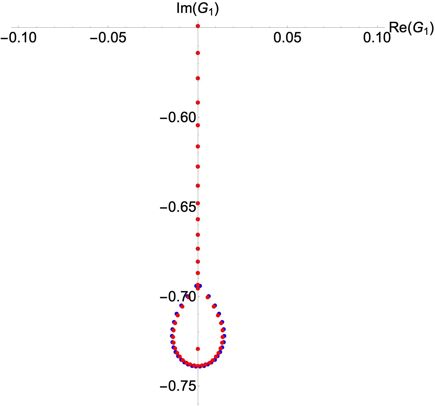
Figure 14: [color online] Blowup of the negative imaginary axis for the $n=200$ truncation showing solutions for $G_{1}$, obtained from (i) the unbiased (blue) and (ii) the asymptotic approximations (red) for $G_{n}$. The blue and red loops are almost the same size, but there is a new red dot that is almost exactly equal to $G_{1}$. These dots also appear in the two other loops at the ends of the three-bladed propeller.

To see more clearly the effect of including the asymptotic behavior of $G_{n}$ in the truncation scheme, we plot the absolute values of the solutions along the negative axis for $n$ ranging from 1 to 200 in Fig. 15. As we see in Fig. 14, there are solutions which are both larger and smaller (in absolute value) than the exact solution. Thus, we do not observe a monotonic behavior of the roots for increasing $n$. However, the the isolated root inside the loop in Fig. 14 is indistinguishable from the exact solution (red line).

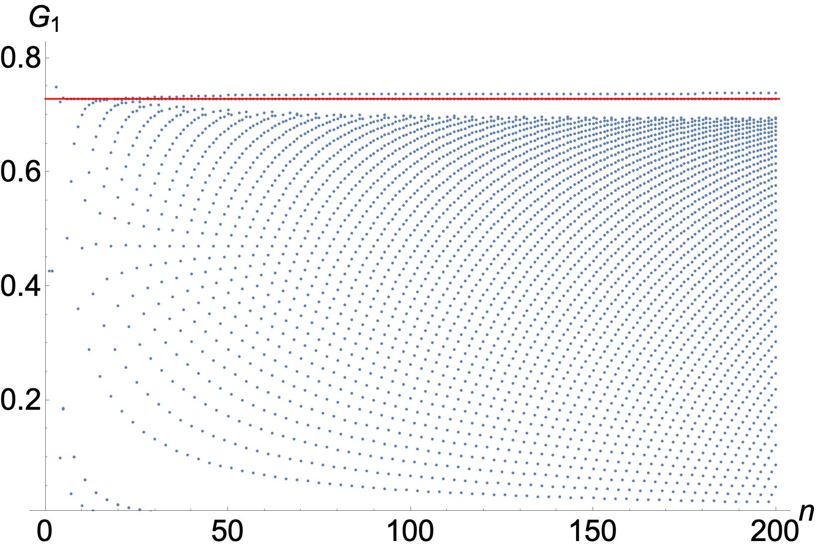
Figure 15: [color online] Absolute values of the solutions for $G_{1}$ on the imaginary axis, obtained using the asymptotic approximation to $G_{n}$ for $n$ ranging from 1 up to 200. The heavy red line shows the exact value of $\big{|}G_{1}\big{|}$.

VI $D=0$ non-Hermitian quartic theory

To understand more broadly the behavior of our truncation schemes, we consider next the quartic Lagrangian

$$\mathcal{L}=-\mbox{$\textstyle{\frac{1}{4}}$}g\phi^{4},$$ (34)

which defines a non-Hermitian massless $\mathcal{PT}$-symmetric theory in zero-dimensional spacetime. The connected one-point Green’s function is for this Lagrangian

$$G_{1}=\int dx\,x\exp(gx^{4}/4)\Big{/}\int dx\,\exp(gx^{4}/4),$$ (35)

where the paths of integration lie inside a $\mathcal{PT}$-symmetric pair of Stokes sectors of angular opening $\tfrac{\pi}{4}$ centered about $-\tfrac{\pi}{4}$ and $-\tfrac{3\pi}{4}$ in the lower-half complex-$x$ plane. Without loss of generality, we set $g=1$ and evaluate these integrals exactly:

$$G_{1}=-2i\sqrt{\pi}\big{/}\Gamma\big{(}\mbox{$\textstyle{\frac{1}{4}}$}\big{)}=-0.977\,741\,07...\,i.$$ (36)

The first eight DS equations for this theory are

$$G_{3} = -G_{1}^{3}-3G_{1}G_{2},$$

$$G_{4} = -3G_{1}G_{3}-3G_{2}^{2}-3G_{1}^{2}G_{2}-1,$$

$$G_{5} = -3G_{1}G_{4}-9G_{2}G_{3}-3G_{1}^{2}G_{3}-6G_{1}G_{2}^{2},$$

$$G_{6} = -3G_{1}G_{5}-12G_{2}G_{4}-3G_{1}^{2}G_{4}-9G_{3}^{2}$$

$$\leavevmode\nobreak\ -18G_{1}G_{2}G_{3}-6G_{2}^{3},$$

$$G_{7} = -3G_{1}G_{6}-15G_{2}G_{5}-3G_{1}^{2}G_{5}-30G_{3}G_{4}$$

$$\leavevmode\nobreak\ -24G_{1}G_{2}G_{4}-18G_{1}G_{3}^{2}-36G_{2}^{2}G_{3},$$

$$G_{8} = -3G_{1}G_{7}-18G_{2}G_{6}-3G_{1}^{2}G_{6}-45G_{3}G_{5}$$

$$\leavevmode\nobreak\ -30G_{1}G_{2}G_{5}-30G_{4}^{2}-60G_{1}G_{3}G_{4}$$

$$\leavevmode\nobreak\ -60G_{2}^{2}G_{4}-90G_{2}G_{3}^{2},$$

$$G_{9} = -3G_{1}G_{8}-21G_{2}G_{7}-3G_{1}^{2}G_{7}-63G_{3}G_{6}$$

$$\leavevmode\nobreak\ -36G_{1}G_{2}G_{6}-105G_{4}G_{5}-90G_{1}G_{3}G_{5}$$

$$\leavevmode\nobreak\ -90G_{2}^{2}G_{5}-60G_{1}G_{4}^{2}-360G_{2}G_{3}G_{4}-90G_{3}^{3},$$

$$G_{10} = -3G_{1}G_{9}-24G_{2}G_{8}-3G_{1}^{2}G_{8}-84G_{3}G_{7}$$ (37)

$$\leavevmode\nobreak\ -42G_{1}G_{2}G_{7}-168G_{4}G_{6}-126G_{1}G_{3}G_{6}$$

$$\leavevmode\nobreak\ -126G_{2}^{2}G_{6}-105G_{5}^{2}-210G_{1}G_{4}G_{5}$$

$$\leavevmode\nobreak\ -630G_{2}G_{3}G_{5}-420G_{2}G_{4}^{2}-630G_{3}^{2}G_{4}.$$

The unbiased approach to solving these equations consists of fixing $n$ and then using successive linear elimination to obtain polynomial equations to be solved numerically for the lowest Green’s functions. However, the procedure is more difficult than for the Hermitian quartic theory in (13) or the non-Hermitian cubic theory in (24) because this elimination process concludes with two polynomials containing not one but two Green’s functions $G_{1}$ and $G_{2}$. That is, we obtain a coupled pair of polynomial equations to solve for $G_{1}$ and $G_{2}$ rather than one polynomial equation in one Green’s function.

For example, the leading truncation ($n=4$) consists of eliminating $G_{3}$ in the second DS equation by substituting the first DS equation into it. We then truncate by setting $G_{3}=G_{4}=G_{5}=\dots=0$ and solve the resulting pair of simultaneous equations. This leads to $G_{1}^{4}=3/2$, and the $\mathcal{PT}$-symmetric solution in the negative-half plane is

$$G_{1}=-i\,\big{(}\mbox{$\textstyle{\frac{3}{2}}$}\big{)}^{1/4}=-1.106\,681\,92...\,i.$$ (38)

This result has an error of $13.2\%$ in comparison with the exact value of $G_{1}$ in (36).

For larger values of $n$ the procedure for solving the pair of polynomial equations is tedious: We multiply each equation by an expression that makes the coefficient of highest power of $G_{1}$ (or $G_{2}$) the same and then subtract the two equations to eliminate this highest-power term. We repeat this process until one of the equations becomes linear in $G_{2}$. We solve this equation for $G_{2}$ and eliminate it algebraically from the other equation. This gives a high-degree polynomial equation for $G_{1}$ that we can finally solve numerically.

The problem with this procedure is that each multiplication introduces spurious roots. However, we find that the final polynomial in powers of $G_{1}$ factors into two polynomials; the roots of one factor are all spurious while the roots of the other factor, which is a polynomial in powers of $G_{1}^{4}$, solve the original pair of equations. The number of roots increases rapidly with $n$ and all roots come in quartets that lie at the vertices of squares in the complex plane. All (nonspurious) roots up to $n=33$ are displayed in Fig. 15. The $\mathcal{PT}$ symmetry of the Lagrangian (34) requires that $G_{1}$ be a negative-imaginary number.

Since we must solve coupled equations for $G_{1}$ and $G_{2}$, we require the exact value of $G_{2}$ in order to calculate the exact values of all of the Green’s functions from (37). The exact value of $G_{2}$ is

$$G_{2}=4\pi\big{/}\Gamma^{2}\big{(}\mbox{$\textstyle{\frac{1}{4}}$}\big{)}-2\Gamma\big{(}\mbox{$\textstyle{\frac{3}{4}}$}\big{)}\big{/}\Gamma\big{(}\mbox{$\textstyle{\frac{1}{4}}$}\big{)}=0.279\,999\,35...\,.$$ (39)

Then, using $G_{1}$ in (36) and $G_{2}$ in (39) we obtain the results given in Table 3.

Table 3: Exact values of 20 Green’s functions for the non-Hermitian quartic theory.

$G_{3}^{\rm exact}=-0.113\,397\,i$	$G_{4}^{\rm exact}=-0.099\,559$
$G_{5}^{\rm exact}=0.128\,446\,i$	$G_{6}^{\rm exact}=0.215\,052\,$
$G_{7}^{\rm exact}=-0.439\,386\,i$	$G_{8}^{\rm exact}=-1.055\,947$
$G_{9}^{\rm exact}=2.912\,307\,i$	$G_{10}^{\rm exact}=9.055\,948$
$G_{11}^{\rm exact}=-31.325\,429\,i$	$G_{12}^{\rm exact}=-119.269\,436$
$G_{13}^{\rm exact}=495.565\,822\,i$	$G_{14}^{\rm exact}=2,231.100\,879$
$G_{15}^{\rm exact}=-10,818.525\,260\,i$	$G_{16}^{\rm exact}=-56,209.003\,831$
$G_{17}^{\rm exact}=311,520.607\,892\,i$	$G_{18}^{\rm exact}=1,834,444.674\,851$
$G_{19}^{\rm exact}=-11,438,011.031\,i$	$G_{20}^{\rm exact}=-75,280,067.556$
$G_{21}^{\rm exact}=521,539,592.082\,i$	$G_{22}^{\rm exact}=3,793,889,240.849$

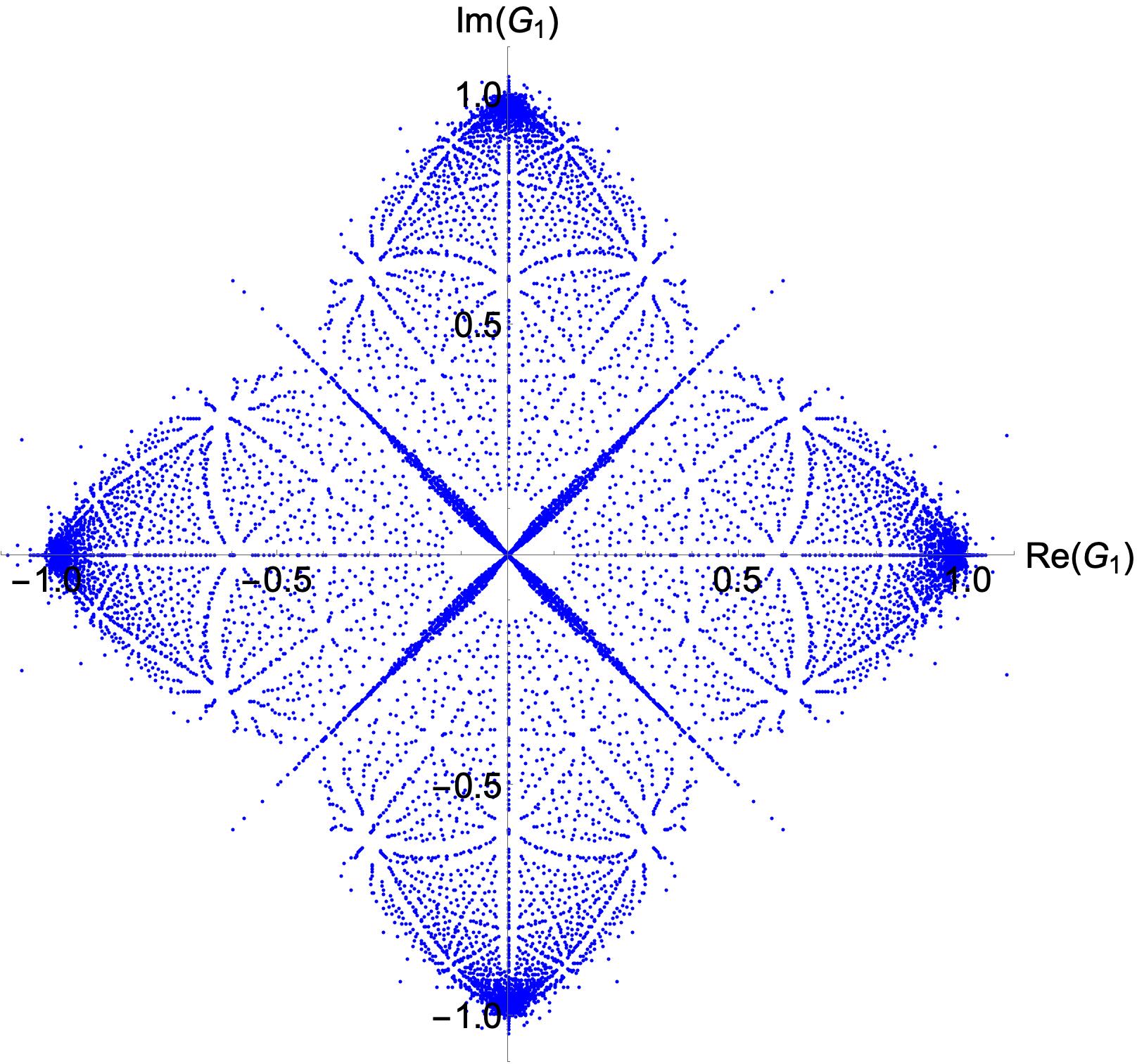
Figure 16: [color online] All solutions for $G_{1}$ in the complex plane up to $n=40$. The roots exhibit fourfold symmetry. However, $\mathcal{PT}$ symmetry requires that $G_{1}$ be negative imaginary, so only the roots on or near the negative-imaginary axis are physically acceptable. The exact value of $G_{1}$, given in (36), lies inside the concentration of roots near $-i$.

VI.1 Asymptotic behavior of $G_{n}$ for large $n$

Inspection of Table 3 shows that the exact values of the odd (even) Green’s functions oscillate in sign as $n$ increases, and that the odd Green’s functions are imaginary, while the even ones are real. Applying Richardson extrapolation to the entries in Table 3, we find that the asymptotic behavior of $G_{n}$ for large $n$ is

$$G_{n}\sim-(n-1)!\,(-i)^{n}r^{n}\quad(n\to\infty),$$ (40)

where $r=0.34640...$. (The overall multiplicative constant in the asymptotic behavior is exactly 1.) This result is similar to the behavior in (32) for the Green’s functions of the non-Hermitian cubic theory.

VII $D=0$ non-Hermitian Quintic Theory

Next, we analyze the quintic $\mathcal{PT}$-symmetric Lagrangian

$$\mathcal{L}=-\tfrac{1}{5}ig\phi^{5}.$$ (41)

The one-point Green’s function is given by

$$G_{1}=\int dx\,x\exp(gx^{5}/5)\Big{/}\int dx\,\exp(gx^{5}/5).$$ (42)

Choosing $\mathcal{PT}$-symmetric Stokes wedges in the negative half-plane and setting $g=1$, we get the exact value

$$G_{1}=-1.078\,653\dots\,.$$ (43)

The first three DS equations that one obtains are

$$G_{4} = -G_{1}^{4}-6G_{2}G_{1}^{2}-4G_{3}G_{1}-3G_{2}^{2}$$

$$G_{5} = -4G_{2}^{3}G_{2}-12G_{1}G_{2}^{2}-6G_{1}^{3}G_{3}-10G_{2}G_{3}$$

$$\quad-4G_{1}G_{4}+i$$

$$G_{6} = -12G_{1}^{2}G_{2}^{2}-4G_{1}^{2}G_{3}-12G_{2}^{3}-36G_{1}G_{2}G_{3}$$ (44)

$$\quad-6G_{1}^{2}G_{4}-10G_{3}^{2}-14G_{2}G_{4}-4G_{1}G_{5}.$$

The first equation for $G_{4}$ contains three unknowns, $G_{1},G_{2}$ and $G_{3}$, so setting $G_{4}=G_{5}=\dots=0$ as a first unbiased truncation means that we must solve three coupled equations. At the next truncation $G_{4}\neq 0$, but all higher $G_{n}=0$. We therefore eliminate $G_{4}$ in terms of $G_{1}$, $G_{2}$, and $G_{3}$, and must solve the next set of three equations. Thus, the solution is complicated. Figure 17 gives a plot of the roots in the complex plane up to $n=11$. These roots exhibit five-fold symmetry.

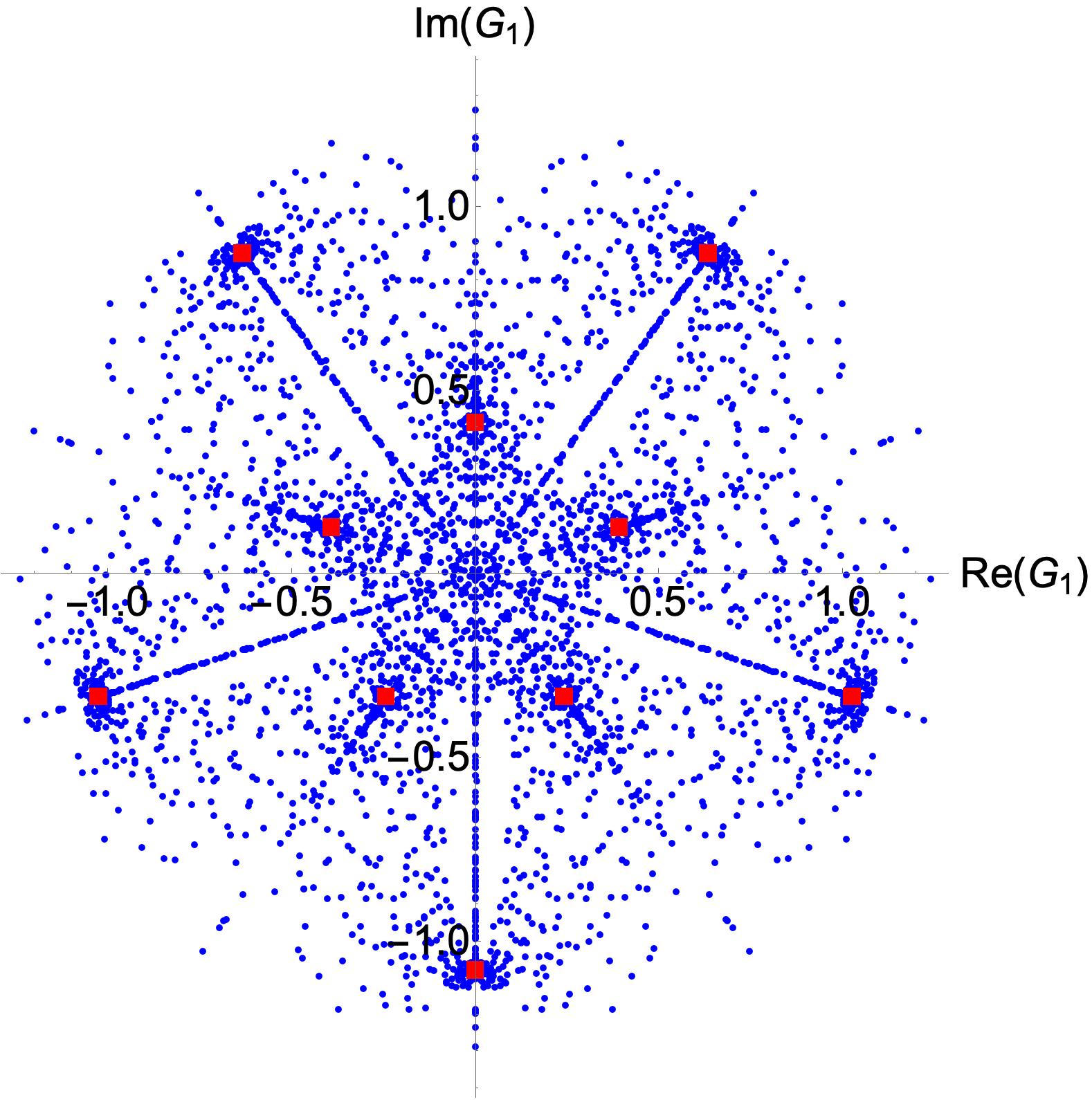
Figure 17: [color online] All solutions for $G_{1}$ in the complex plane, up to $n=11$. The roots exhibit fivefold symmetry but $\mathcal{PT}$ symmetry requires that $G_{1}$ be negative imaginary, so only the roots on or near the negative-imaginary axis are physically acceptable. The exact value of $G_{1}$, given in (43), lies inside the concentration of roots near $-i$.

We observe ten concentrations of roots. One can understand this as follows: Associated with the Lagrangian (41) are five Stokes sectors that define the regions of convergence of the integral (42) in the complex plane (Stokes sectors). Thus, there are ten possible distinct paths of integration in the complex plane, each of which lead to different values of $G_{1}$. Aside from the imaginary value in (43), there is another imaginary $\mathcal{PT}$-symmetric solution from $\mathcal{PT}$-symmetric (left-right symmetric) integration in the upper-half plane that gives $G_{1}=0.4120\dots i$. The other possible complex values of the integral for $G_{1}$ are $\pm 0.392\dots+0.127\dots i$, $\pm 0.242\dots-0.333\dots i$, $\pm 0.634\dots+0.872\dots i$, and $\pm 1.025\dots-0.333\dots i$. These ten values for $G_{1}$ are plotted as red squares on Fig. 17, and correspond to the dense regions of solutions.

This feature is a general one: for the quartic and cubic systems discussed in the previous sections, an analysis of all possible paths of integration in each case results in all possible solutions of the Green’s functions being represented in the complex plane.

VIII $D=0$ Hermitian Sextic Theory

Here we consider the zero-dimensional model described by the massless Lagrangian

$$\mathcal{L}=\frac{1}{6}g\phi^{6}.$$ (45)

The first two Green’s functions are given by

$$G_{1} = \int d\phi\phi e^{-\phi^{6}/6}\Big{/}\int d\phi e^{-\phi^{6}/6}$$

$$G_{2} = \int d\phi\phi^{2}e^{-\phi^{6}/6}\Big{/}\int d\phi e^{-\phi^{6}/6},$$ (46)

where $g=1$. The paths of integration must be specified, and there are six distinct regions of convergence bounded by the Stokes lines at $\tfrac{\pi}{12}+n\tfrac{\pi}{6}$, so there are 15 possible combinations of integration paths. Thus, there are 15 different theories associated with the Lagrangian (45).

The first DS equation is complicated and contains five unknowns:

$$G_{5} = -G_{1}^{5}-10G_{1}^{3}G_{2}-10G_{1}^{2}G_{3}-15G_{1}G_{2}^{2},$$ (47)

$$\qquad-5G_{1}G_{4}-10G_{2}G_{3}\,,$$

and, in general, a complete solution of the DS equations would require that we solve four coupled polynomial equations at each truncation level.

To reduce the calculational complexity, we restrict the system to be parity symmetric, so that all odd Green’s functions vanish. The Hermitian sextic theory has an integration path along the real axis. The exact value of $G_{2}$, obtained by integrating (46) along this path gives

$$G_{2}=0.578\,616\,519\dots.$$ (48)

However, there are two other choices for the integration path that also respect parity symmetry and give rise to the values

$$G_{2}=-0.2893\dots\pm 0.5010\dots i.$$ (49)

Imposing parity symmetry on the first DS equation (47) gives the trivial equation $0=0$. The first five (nontrivial) DS equations link the even-$n$ Green’s functions to others of higher order:

$$G_{6} = -15G_{2}^{3}-15G_{2}G_{4}+1,$$

$$G_{8} = -60G_{2}^{4}-165G_{2}^{2}G_{4}-35G_{4}^{2}-25G_{2}G_{6},$$

$$G_{10} = -120G_{2}^{5}-1200G_{2}^{3}G_{4}-1150G_{2}G_{4}^{2}-365G_{2}^{2}G_{6}$$

$$-205G_{4}G_{6},$$

$$G_{12} = -4200G_{2}^{4}G_{4}-16800G_{2}^{2}G_{4}^{2}-4550G_{4}^{3}$$

$$-3360G_{2}^{3}G_{6}-8470G_{2}G_{4}G_{6}-455G_{6}^{2}$$

$$-645G_{2}^{2}G_{8}-460G_{4}G_{8}-45G_{2}G_{10},$$

$$G_{14} = -100800G_{2}^{3}G_{4}^{2}-168000G_{2}G_{4}^{3}-15120G_{2}^{4}G_{6}$$

$$-151200G_{2}^{2}G_{4}G_{6}-76020G_{4}^{2}G_{6}-23310G_{2}G_{6}^{2}$$

$$-7200G_{2}^{3}G_{8}-22680G_{2}G_{4}G_{8}-2910G_{6}G_{8}$$

$$-1005G_{2}^{2}G_{10}-875G_{4}G_{10}-55G_{2}G_{12}.$$

As before, we truncate the DS equations by taking at each step a pair of successive equations and setting the highest-order connected Green’s functions to zero. This constitutes a truncation of order $n$. The results for $G_{2}$ up to $n=30$ (where we solve the equations $G_{64}=G_{66}=0$) are shown in Fig. 18.

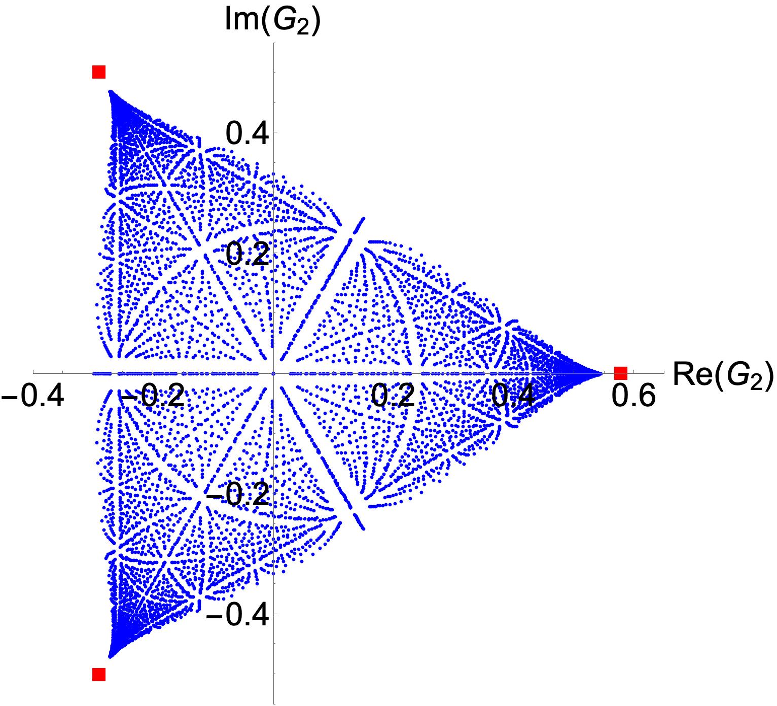
Figure 18: [color online] Roots of the DS equations for the Hermitian sextic case obtained by means of the unbiased truncation scheme. There are three concentrations of solutions for $G_{2}$ that differ from the exact values in (48) and (49) (red squares) by a few percent.

Like the quartic case, the roots converge monotonically to points near the three exact values of $G_{2}$ in (48) and (49). Richardson extrapolation gives the limiting values of the truncated sequences and these limiting values differ from the exact values by 6% (see Fig. 19).

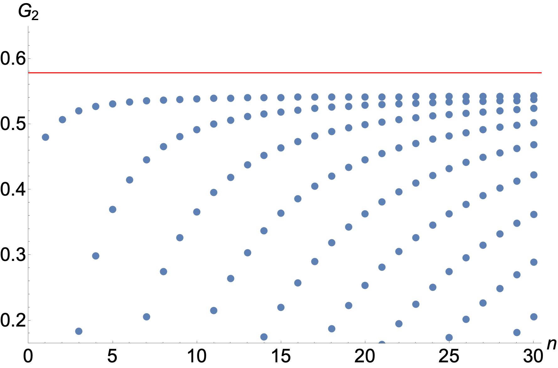
Figure 19: [color online] Positive values of the roots of the SD equations for the Hermitian sextic case (dots). The exact value of $G_{2}=0.578\,616\dots$ is indicated by the red line and the DS results converge to a number that differs from the exact value by about 20%.

IX Conclusions

In this paper we have studied the effectiveness of the DS equations as a way to calculate the Green’s functions of a quantum field theory. We have examined the DS equations for zero-dimensional field theories only because in this case we can evaluate the integral representations of the Green’s functions exactly and then compare these exact results with the approximants provided by the DS equations. We find that while the Green’s functions exactly satisfy the infinite system of coupled DS equations, the DS equations alone cannot be used to obtain accurate results for the Green’s functions.

The reason for this is that Green’s functions are expressed in terms of moments of the functional integral that specifies the partition function $Z$ of the quantum field theory. However, the DS equations are derived by functional differentiation of the partition function. While differentiation preserves local information, the global information in the functional integral, which is required to specify the Green’s functions uniquely, is lost.

As a trivial example, consider the function

$$f(x)=\tfrac{1}{4}x^{3}+\tfrac{2}{x}\quad(1\leq x\leq 2).$$ (50)

We may differentiate $f(x)$ once to obtain a differential equation satisfied by $f(x)$:

$$f^{\prime}(x)+\tfrac{f(x)}{x}=x^{2}.$$ (51)

However, while this equation describes the local behavior of $f(x)$ at each point $x$, we have lost the global boundary data needed to recover the original function $f(x)$: The general solution to this differential equation,

$$f(x)=\tfrac{1}{4}x^{3}+\tfrac{C}{x},$$ (52)

contains an arbitrary constant. However, if we specify the boundary data $f(2)=3$, this determines that $C=2$ and we have recovered $f(x)$ in (50).

As explained in Sec. III, deriving the DS equations involves a somewhat more complicated differentiation process. However, the resulting coupled infinite system of DS equations is so complicated that it obscures the simple fact that in the differentiation process some information has been lost. For example, the functional-integral representation of the partition function exists because the path of functional integration terminates as $|\phi|\to\infty$ inside a pair of Stokes sectors in complex-$\phi$ space ($\phi$ is the integration variable). Because there are many possible pairs of sectors that give a convergent functional integral, when we solve the DS equations we find all possible solutions to the DS equations corresponding to all possible pairs of Stokes sectors, some corresponding to Hermitian theories and others corresponding to non-Hermitian theories (both $\mathcal{PT}$-symmetric and non-$\mathcal{PT}$-symmetric). For instance, in Fig. 17 there are 10 concentrations of roots corresponding to the ten possible paths of integration for a quintic field theory. The DS equations weight each of these theories equally.

There is even more loss of information than this. As we have shown, solving the DS equations is a two-step process. First, we truncate the infinite triangular system of DS equations, but when we do so, the resulting finite system always has more Green’s functions than equations and is therefore indeterminate. Next, to obtain a closed system of coupled equations we perform a further truncation in which we set the highest Green’s functions to 0. (In this paper we call this truncation procedure unbiased.) There are other truncation possibilities as well, but in all cases we find that as we include more and more DS equations, the solutions do not converge to the already known exact values of the Green’s functions.

Nevertheless, a remarkable feature of the unbiased approach is that for all five theories studied in this paper, as we include more DS equations, the approximate Green’s functions actually converge to limiting values, and these limiting values are fairly accurate – several percent off from the exact values for all of the Green’s functions for all of the theories corresponding to the possible pairs of Stokes sectors, as discussed above.

Finally, we have found a successful way to insert the missing information back into the DS equations. Instead of using the unbiased ansatz of setting the higher unknown Green’s functions to zero, we replace $G_{n}$ by its asymptotic behavior for large $n$. This procedure gives new and extremely accurate numerical results for the Green’s functions (many decimal places). However, it does not eliminate all of the spurious theories associated with different pairs of Stokes sectors; this can only be done by imposing external additional conditions on the DS equations such as spectral positivity. The use of the asymptotic behavior of $G_{n}$ for large $n$ suggests a new and interesting general mathematical problem that has not been studied previously in this context, namely, finding the asymptotic behavior of many-legged Green’s functions in higher-dimensional field theories.

One last remark: A simple way to force the DS equations to give sequences of approximants that converge to the exact values of the Green’s functions is to require that the Green’s functions all have formal weak-coupling expansions in powers of a coupling constant. This approach has been known for a long time R9 . To illustrate this idea we return to the trivial differential-equation example above. We can demand that the solution to the differential equation (51) be entire; that is, that the solution $f(x)$ have a convergent Taylor-series representation. This condition uniquely determines the unknown constant $C$ in (52): $C=0$. Unfortunately, it does not recover the original function $f(x)$ in (50), which is singular at the origin. Similarly, if we require that all Green’s functions have weak-coupling expansions, we immediately exclude the possibility of using the DS equations to calculate Green’s functions having nonperturbative behavior. Indeed, if we ignore the possibility of nonperturbative behavior, there is no reason to consider the DS equations at all because Feynman diagrams give the perturbative representations of Green’s functions.

- (1) C. M. Bender, C. Karapoulitidis, and S. P. Klevansky, Underdetermined Dyson-Schwinger equations, Phys. Rev. Lett. 130, 101602 (2023).
- (2) Early low-dimensional studies of the DS equations may be found in C. M. Bender, G. S. Guralnik, R. W. Keener, and K. Olaussen, Numerical study of truncated Green’s function equations, Phys. Rev. D 14, 2590 (1976); C. M. Bender, K. A. Milton, and V. M. Savage, Solution of Schwinger-Dyson Equations for PT-Symmetric Quantum Field Theory, Phys. Rev. D 62, 085001 (2000); C. M. Bender and S. P. Klevansky, Families of particles with different masses in -symmetric quantum field theory, Phys. Rev. Lett. 105, 031601 (2010).
- (3) We thank S. Coleman for a lengthy discussion of this history.
- (4) F. J. Dyson, The matrix in quantum electrodynamics, Phys. Rev. 75, 1736 (1949).
- (5) J. Schwinger, On the Green’s functions of quantized fields I, Proc. Nat. Acad. Sci. 37, 452 (1951).
- (6) J. Schwinger, On the Green’s functions of quantized fields II, Proc. Nat. Acad. Sci. 37, 455 (1951).
- (7) See discussion of Richardson extrapolation in C. M. Bender and S. A. Orszag, Advanced Mathematical Methods for Scientists and Engineers (Springer-Verlag, New York, 1999), Chap. 8.
- (8) See discussion of Wilkinson polynomials in C. M. Bender and S. A. Orszag, Ibid., Chap. 7.
- (9) C. M. Bender, F. Cooper, and L. M. Simmons, Jr., Nonunique solution to the Schwinger-Dyson equations, Phys. Rev. D 39, 2343 (1989). This idea has been rediscovered very recently by W. Li, Taming Dyson-Schwinger equations with null states, arXiv: 2303.10978 and Solving anharmonic oscillator with null states, arXiv: 2305.15992.