New Method for Measuring the Ratio $\mu_{p}G_{E}/G_{M}$ Based on the Polarization Transfer from the Initial Proton to the Final Electron in the $e\vec{p}\to\vec{e}p$ Process

Abstract

In this letter, we propose a new method for measuring the Sachs form factors ratio ($R=\mu_{p}G_{E}/G_{M}$) based on the transfer of polarization from the initial proton to the final electron in the elastic $e\vec{p}\to\vec{e}p$ process, in the case when the axes of quantization of spins of the target proton at rest and of the scattered electron are parallel, i.e., when an electron is scattered in the direction of the spin quantization axis of the proton target. To do this, in the kinematics of the SANE collaboration experiment (2020) on measuring double spin asymmetry in the $\vec{e}\vec{p}\to ep$ process, using Kelly (2004) and Qattan (2015) parametrizations, a numerical analysis was carried out of the dependence of the longitudinal polarization degree of the scattered electron on the square of the momentum transferred to the proton, as well as on the scattering angles of the electron and proton. It is established that the difference in the longitudinal polarization degree of the final electron in the case of conservation and violation of scaling of the Sachs form factors can reach 70%. This fact can be used to set up polarization experiments of a new type to measure the ratio $R$.

Introduction.—Experiments on the study of electric ($G_{E}$) and magnetic ($G_{M}$) proton form factors, the so-called Sachs form factors (SFF), have been conducted since the mid-1950s Hofstadter1958 in the process of elastic scattering of unpolarized electrons off a proton. At the same time, all experimental data on the behavior of SFF were obtained using the Rosenbluth technique (RT) based on the use of the Rosenbluth cross section (in the approximation of the one-photon exchange) for the $ep\to ep$ process in the rest frame of the initial proton Rosen

$$\frac{d\sigma}{d\Omega_{e}}=\frac{\alpha^{2}E_{2}\cos^{2}(\theta_{e}/2)}{4E_{1}^{3}\sin^{4}(\theta_{e}/2)}\frac{1}{1+\tau_{p}}\left(G_{E}^{2}+\frac{\tau_{p}}{\varepsilon}\,G_{M}^{2}\right).$$ (1)

Here $\tau_{p}=Q^{2}/4m^{2}$, $Q^{2}=4E_{1}E_{2}\sin^{2}(\theta_{e}/2)$ is the square of the 4-momentum transferred to the proton; $m$ is the mass of the proton; $E_{1}$ and $E_{2}$ are the energies of the initial and final electrons; $\theta_{e}$ is the electron scattering angle; $\varepsilon=[1+2(1+\tau_{p})\tan^{2}(\theta_{e}/2)]^{-1}$ is the degree of linear (transverse) polarization of the virtual photon Dombey ; Rekalo74 ; AR ; GL97 ; and $\alpha=1/137$ is the fine structure constant.

For large values of $Q^{2}$, as follows from formula (1), the main contribution to the cross section of the $ep\to ep$ process is given by the term proportional to $G_{M}^{\,2}$, which is already at $Q^{2}\geqslant 2\leavevmode\nobreak\ \mbox{GeV}^{2}$ leads to significant difficulties in extracting the contribution of $G_{E}^{\,2}$ ETG15 ; Punjabi2015 .

With the help of RT, the dipole dependence of the SFF on $Q^{2}$ in the region $Q^{2}\leqslant 6\leavevmode\nobreak\ \mbox{GeV}^{2}$ was established ETG15 ; Punjabi2015 . As it turned out, $G_{E}$ and $G_{M}$ are related by the scaling ratio $G_{M}\approx\mu_{p}G_{E}$ ($\mu_{p}=2.79$ – the magnetic moment of the proton), and for their ratio $R\equiv\mu_{p}G_{E}/G_{M}$, the approximate equality $R\approx 1$ is valid.

In the paper of Akhiezer and Rekalo Rekalo74 , a method for measuring the ratio of $R$ is proposed based on the phenomenon of polarization transfer from the initial electron to the final proton in the $\vec{e}p\to e\vec{p}$ process. Precision JLab experiments Jones00 ; Gay01 ; Gay02 , using this method, found a fairly rapid decrease in the ratio of $R$ with an increase in $Q^{2}$, which indicates a violation of the dipole dependence (scaling) of the SFF. In the range $0.4\leavevmode\nobreak\ \mbox{GeV}^{2}\leqslant Q^{2}\leqslant 5.6\leavevmode\nobreak\ \mbox{GeV}^{2}$, as it turned out, this decrease is linear. Next, more accurate measurements of the ratio $R$ carried out in Pun05 ; Puckett10 ; Puckett12 ; Puckett17 ; Qattan2005 in a wide area in $Q^{2}$ up to $8.5\leavevmode\nobreak\ \mbox{GeV}^{2}$ using both the Akhiezer–Rekalo method Rekalo74 and the RT Qattan2005 , only confirmed the discrepancy of the results.

In the SANE collaboration experiment Liyanage2020 (2020), the values of $R$ were obtained by the third method Dombey ; Donnelly1986 by extracting them from the results of measurements of double spin asymmetry in the $\vec{e}\vec{p}\to ep$ process in the case, when the electron beam and the proton target are partially polarized. The extracted values of $R$ in Liyanage2020 are consistent with the experimental results Jones00 ; Gay01 ; Gay02 ; Pun05 ; Puckett10 ; Puckett12 ; Puckett17 .

In JETPL2008 ; JETPL18 ; JETPL19 ; JETPL2021 ; PEPAN2022 ; JETPL2022 , the 4th method of measuring $R$ is proposed based on the transfer of polarization from the initial proton to the final one in the $e\vec{p}\to e\vec{p}$ process in the case when their spins are parallel, i.e. when the proton is scattered in the direction of the quantization axis of the spin of the resting proton target.

In this paper, the 5th method of measuring the ratio of $R$ is proposed based on the transfer of polarization from the initial proton to the final electron in the process $e\vec{p}\to\vec{e}p$ in the case when their spins are parallel, i.e. when the electron is scattered in the direction of the spin quantization axes of the resting proton target.

The helicity and diagonal spin bases.—The spin 4-vector $s=(s_{0},\mbox{\boldmath$s$})$ of the fermion with 4-momentum $p$ ($p^{2}=m^{2})$ satisfying the conditions of orthogonality ($sp=0$) and normalization ($s^{2}=-1$), is given by

$$s=(s_{0},\mbox{\boldmath$s$}),\quad s_{0}=\frac{\mbox{\boldmath$c$}\,\mbox{\boldmath$p$}}{m},\quad\mbox{\boldmath$s$}=\mbox{\boldmath$c$}+\frac{\,(\mbox{\boldmath$c$}\,\mbox{\boldmath$p$})\,\mbox{\boldmath$p$}}{m(p_{0}+m)\,}\;,$$ (2)

where $c$ ($\mbox{\boldmath$c$}^{2}=1$) is the axis of spin quantization.

Expressions (2) allow us to determine the spin 4-vector $s=(s_{0},\mbox{\boldmath$s$})$ by a given 4-momentum $p=(p_{0},\mbox{\boldmath$p$})$ and 3-vector $c$. On the contrary, if the 4-vector $s$ is known, then the spin quantization axis $c$ is given by

$$\mbox{\boldmath$c$}=\mbox{\boldmath$s$}-\frac{s_{0}}{p_{0}+m}\,\mbox{\boldmath$p$},$$ (3)

i.e. $c$ and $s$ for a given $p$ uniquely define each other.

At present, the most popular in high-energy physics is the helicity basis Jacob , in which the spin quantization axis is directed along the momentum of the particle ($\mbox{\boldmath$c$}=\mbox{\boldmath$n$}=\mbox{\boldmath$p$}/|\mbox{\boldmath$p$}|$), while the spin 4-vector (2) defined as

$$s=(s_{0},\mbox{\boldmath$s$})=(|\mbox{\boldmath$v$}|,v_{0}\,\mbox{\boldmath$n$}),$$ (4)

where $v_{0}$ and $v$ are the time and space components of the 4-velocity vector $v=p/m$ ($v^{2}=1$).

For the process under consideration

$$e(p_{1})+p\,(q_{1},s_{p_{1}})\to e(p_{2},s_{e_{2}})+p\,(q_{2}),$$ (5)

where $p_{1}$, $q_{1}$ ($p_{2}$, $q_{2}$) are the 4-momenta of the initial (final) electrons and protons with masses $m_{0}$ and $m$, it is possible to project the spins of the initial proton and the final electron in one common direction given by FIF70 ; GL

$$\mbox{\boldmath$a$}=\mbox{\boldmath$p$}_{2}/p_{20}-\mbox{\boldmath$q$}_{1}/q_{10}.$$ (6)

Since the common axis of spin quantization (6) defines the spin basis and is the difference of two three-dimensional vectors, the geometric image of which is the diagonal of the parallelogram, it is natural to call it the diagonal spin basis (DSB). In it, the spin 4-vectors of the initial proton $s_{p_{1}}$ and the final electron $s_{e_{2}}$ are given by

$$s_{p_{1}} = \frac{m^{2}p_{2}-(q_{1}p_{2})q_{1}}{m\sqrt{(q_{1}p_{2})^{2}-m^{2}m_{0}^{2}}},$$ (7)

$$s_{e_{2}} = \frac{(q_{1}p_{2})p_{2}-m_{0}^{2}q_{1}}{m_{0}\sqrt{(q_{1}p_{2})^{2}-m^{2}m_{0}^{2}}}.$$ (8)

Note that in the papers JETPL2008 ; JETPL18 ; JETPL19 ; JETPL2021 ; PEPAN2022 ; JETPL2022 was used the analogous DSB for the initial and final protons (with a common spin quantization axis $\mbox{\boldmath$a$}=\mbox{\boldmath$q$}_{2}/q_{20}-\mbox{\boldmath$q$}_{1}/q_{10}$) Sik84 ; GS98 .

In the laboratory frame (LF), where the initial proton rests, $q_{1}=(m,\mbox{\boldmath$0$})$, the spin 4-vectors (7), (8) reduces to

$$s_{p_{1}}=(0,\mbox{\boldmath$n_{2}$})\,,\;s_{e_{2}}=(|\mbox{\boldmath$v_{2}$}|,v_{20}\,\mbox{\boldmath$n_{2}$})\,,$$ (9)

where $\mbox{\boldmath$n$}_{2}=\mbox{\boldmath$p_{2}$}/|\mbox{\boldmath$p$}_{2}|$, $v_{2}=(v_{20},\mbox{\boldmath$v_{2}$})=p_{2}/m_{0}$.

Using the explicit form of the spin 4-vectors $s_{p_{1}}$ and $s_{e_{2}}$ (9) and formulas (3) or (6), it is easy to verify that the quantization axes of the initial proton and the final electron spins in the LF have the same form and coincide with the direction of the final electron momentum

$$\mbox{\boldmath$a$}=\mbox{\boldmath$c$}=\mbox{\boldmath$c$}_{p_{1}}=\mbox{\boldmath$c$}_{e_{2}}=\mbox{\boldmath$n$}_{2}=\mbox{\boldmath$p_{2}$}/|\mbox{\boldmath$p$}_{2}|\,.$$ (10)

In the ultrarelativistic limit, when the electron mass can be neglected (i.e. at $p_{10},p_{20}\gg m_{0}$), the spin 4-vectors (7), (8) reduces to

$$s_{p_{1}}=\frac{m^{2}p_{2}-(q_{1}p_{2})\,q_{1}}{m(q_{1}p_{2})},\qquad s_{e_{2}}=\frac{p_{2}}{m_{0}}\,.$$ (11)

Below, in the ultrarelativistic limit, we present the main kinematic relations used in conducting numerical calculations of polarization effects in the $e\vec{p}\to\vec{e}p$ process in the LF.

Kinematics.—The energies of the final electron $E_{2}$ and proton $E_{2p}$ are connected in the LF with the square of the momentum transferred to the proton $Q^{2}=-q^{2}$, $q^{2}=(q_{2}-q_{1})^{2}$ as follows

$$E_{2}=E_{1}-Q^{2}/2m,\qquad E_{2p}=m+Q^{2}/2m,$$ (12)

$$E_{2}=E_{1}-2m\tau_{p},\qquad E_{2p}=m(1+2\tau_{p}).$$ (13)

The dependence of $E_{2}$ and $Q^{2}$ on the scattering angle of the electron $\theta_{e}$ in the LF has the form

$$E_{2}(\theta_{e}) = \frac{E_{1}}{1+(2E_{1}/m)\,\sin^{2}(\theta_{e}/2)},$$ (14)

$$Q^{2}(\theta_{e}) = \frac{4E_{1}^{\,2}\sin^{2}(\theta_{e}/2)}{1+(2E_{1}/m)\sin^{2}(\theta_{e}/2)},$$ (15)

where $\cos(\theta_{e})=\mbox{\boldmath$p$}_{1}\mbox{\boldmath$p$}_{2}/|\mbox{\boldmath$p$}_{1}||\mbox{\boldmath$p$}_{2}|$.

The dependence of $E_{2p}$ and $Q^{2}$ on the scattering angle of the proton $\theta_{p}$ in the LF has the form

$$E_{2p}(\theta_{p}) = m\,\frac{(E_{1}+m)^{2}+E_{1}^{\,2}\cos^{2}(\theta_{p})}{(E_{1}+m)^{2}-E_{1}^{\,2}\cos^{2}(\theta_{p})}\,,$$ (16)

$$Q^{2}(\theta_{p}) = \frac{4m^{2}E_{1}^{\,2}\cos^{2}(\theta_{p})}{(E_{1}+m)^{2}-E_{1}^{\,2}\cos^{2}(\theta_{p})}\,,$$ (17)

where $\cos(\theta_{p})=\mbox{\boldmath$p$}_{1}\mbox{\boldmath$q$}_{2}/|\mbox{\boldmath$p$}_{1}||\mbox{\boldmath$q$}_{2}|$.

The dependence of the scattering angles $\theta_{e}$ and $\theta_{p}$ on $E_{1}$ and $Q^{2}$ has the form

$$\theta_{e}=\arccos{\left(1-\frac{Q^{2}}{2E_{1}E_{2}}\right)},$$ (18)

$$\theta_{p}=\arccos{\left(\frac{E_{1}+m}{E_{1}}\sqrt{\frac{\tau_{p}}{1+\tau_{p}}}\;\right)}.$$ (19)

In the elastic $ep\to ep$ process an electron can be scattered by an angle of $0^{\circ}\leqslant\theta_{e}\leqslant 180^{\circ}$, while the scattering angle of the proton $\theta_{p}$ varies from $90^{\circ}$ to $0^{\circ}$ AR . Possible values of $Q^{2}$ lie in the range $0\leqslant Q^{2}\,\leqslant Q^{2}_{max}$, where

$$Q^{2}_{max}=\frac{4mE_{1}^{\,2}}{(m+2E_{1})}\,.$$ (20)

The results of calculations of the dependence of the scattering angles of the electron and proton on the square of the momentum transferred to the proton $Q^{2}$ in the $ep\to ep$ process at electron beam energies $E_{1}=4.725$ and $5.895\leavevmode\nobreak\ \mbox{GeV}$ in the SANE collaboration experiment Liyanage2020 are presented by the graphs in Figure 1. They correspond to lines with labels $\theta_{e4}$, $\theta_{p4}$ and $\theta_{e5}$, $\theta_{p5}$.

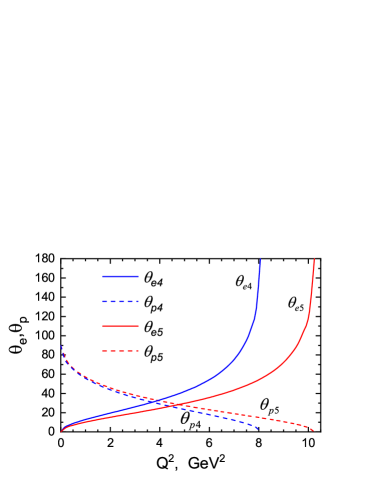
Figure 1: $Q^{2}$-dependence of the scattering angles of the electron $\theta_{e}$ and the proton $\theta_{p}$ (in degrees) at electron beam energies in the experiment Liyanage2020 . The lines $\theta_{e4}$, $\theta_{p4}$ ($\theta_{e5}$, $\theta_{p5}$) correspond to $E_{1}=4.725$ ($5.895$) GeV.

Information about the electron and proton scattering angles (in radians) at electron beam energies and values of $Q^{2}$ in the experiment Liyanage2020 is presented in Table 1. It also contains the corresponding values for $Q^{2}_{max}$ (20).

Table 1: The scattering angles of the electron $\theta_{e}$ and proton $\theta_{p}$ (in radians) at electron beam energies $E_{1}=4.725$ and $5.895\leavevmode\nobreak\ \mbox{GeV}$ and values $Q^{2}$ equal to $2.06$ and $5.66\leavevmode\nobreak\ \mbox{GeV}^{2}$.

$E_{1}$ (GeV)	$Q^{2}$ ($\mbox{GeV}^{2}$)	$\theta_{e}(rad)$	$\theta_{p}(rad)$	$Q^{2}_{max}$ ($\mbox{GeV}^{2}$)
5.895	2.06	0.27	0.79	10.247
5.895	5.66	0.59	0.43	10.247
4.725	2.06	0.35	0.76	8.066
4.725	5.66	0.86	0.35	8.066

Cross section of the $e\vec{p}\to\vec{e}p$ process.—In the one-photon exchange approximation, the differential cross section of the process (5), calculated in an arbitrary reference frame in the DSB (7), (8), reads

$$\frac{d\sigma_{e\vec{p}\to\vec{e}p}}{dt} = \frac{\pi\alpha^{2}}{2\lambda_{s}(1+\tau_{p})}\,\frac{|{T}|^{2}}{t^{2}},$$ (21)

$$|T|^{2} = I_{0}+\lambda_{p_{1}}\lambda_{e_{2}}I_{1},$$ (22)

$$I_{0} = G_{E}^{\,2}Y_{1}+\tau_{p}\,G_{M}^{\,2}Y_{2},$$ (23)

$$I_{1} = \tau_{p}(\,G_{E}G_{M}Y_{3}+G_{M}^{\,2}Y_{4}),$$ (24)

where $t=q^{2}$, $\lambda_{s}=4((p_{1}q_{1})^{2}-m_{0}^{2}\,m^{2})$, $\lambda_{p_{1}}$ ($\lambda_{e_{2}}$) – the degree of polarization of the initial proton (of the final electron).

Here the functions $Y_{i}$ ($i=1,\ldots 4$) defined as

$$Y_{1} = (p_{+}q_{+})^{2}+q_{+}^{2}q_{-}^{2},$$ (25)

$$Y_{2} = (p_{+}q_{+})^{2}-q_{+}^{2}(q_{-}^{2}+4m_{0}^{2}),$$ (26)

$$-Y_{3} = 2\,\kappa\,m^{2}\,((p_{+}q_{+})^{2}+q_{+}^{2}(q_{-}^{2}-4\,m_{0}^{2}\,))\,z^{2},$$ (27)

$$Y_{4} = 2\,(m^{2}p_{+}q_{+}-\kappa q_{+}^{2})(\kappa p_{+}q_{+}-m_{0}^{2}\,q_{+}^{2})z^{2},\leavevmode\nobreak\ \leavevmode\nobreak\ \leavevmode\nobreak\$$

$$z=(\kappa^{2}-m^{2}m_{0}^{2})^{-1/2}\,,\;\kappa=q_{1}p_{2}.$$

Expression (22) for $|T|^{2}$ can be written as

$$|T|^{2}=I_{0}+\lambda_{p_{1}}\lambda_{e_{2}}I_{1}=I_{0}\,(1+\lambda_{e_{2}}\lambda_{e_{2}}^{f}).$$ (29)

Then the value of $\lambda_{e_{2}}^{f}$ in (29) is the longitudinal polarization degree transferred from the initial proton to the final electron in the $e\vec{p}\to\vec{e}p$ process

$$\lambda_{e_{2}}^{f}=\lambda_{p_{1}}\frac{I_{1}}{I_{0}}=\lambda_{p_{1}}\frac{\tau_{p}(G_{E}G_{M}Y_{3}+G_{M}^{\,2}Y_{4})}{G_{E}^{\,2}Y_{1}+\tau_{p}G_{M}^{\,2}Y_{2}}.$$ (30)

Dividing the numerator and denominator in the last expression by $Y_{1}G_{M}^{\,2}$ and introducing the experimentally measured ratio $R\equiv\mu_{p}G_{E}/G_{M}$, we get

$$\lambda_{e_{2}}^{f}=\lambda_{p_{1}}\,\frac{\mu_{p}\tau_{p}\,((Y_{3}/Y_{1})R+\mu_{p}(Y_{4}/Y_{1}))}{R^{\,2}+\mu_{p}^{2}\,\tau_{p}\,(Y_{2}/Y_{1})\,}.$$ (31)

Inverting relation (31), we obtain a quadratic equation with respect to $R$:

$$\alpha_{0}R^{2}-\alpha_{1}R+\alpha_{0}\alpha_{3}-\alpha_{2}=0$$ (32)

with the coefficients:

$$\alpha_{0}=\lambda_{e_{2}}^{f}/\lambda_{p_{1}},\;\alpha_{1}=\tau_{p}\,\mu_{p}\,Y_{3}/Y_{1},$$ (33)

$$\alpha_{2}=\tau_{p}\,\mu_{p}^{2}\,Y_{4}/Y_{1},\;\alpha_{3}=\tau_{p}\,\mu_{p}^{2}\,Y_{2}/Y_{1}.$$

Solutions to equation (32) have the form:

$$R=\frac{\alpha_{1}\pm\sqrt{\alpha_{1}^{2}-4\alpha_{0}(\alpha_{0}\alpha_{3}-\alpha_{2})}}{2\alpha_{0}}.$$ (34)

They allow us to extract the ratio $R$ from the results of an experiment to measure the polarization transferred to the electron $\lambda_{e_{2}}^{f}$ in the $e\vec{p}\to\vec{e}p$ process in the case when the scattered electron moves in the direction of the spin quantization axis of the initial resting proton.

In the ultrarelativistic limit, when the electron mass can be neglected, expressions (25)–(New Method for Measuring the Ratio $\mu_{p}G_{E}/G_{M}$ Based on the Polarization Transfer from the Initial Proton to the Final Electron in the $e\vec{p}\to\vec{e}p$ Process) for $Y_{i}$ ($i=1,\ldots 4$) in LF are given by

$$Y_{1}=8m^{2}(2E_{1}E_{2}-mE_{-}),$$ (35)

$$Y_{2}=8m^{2}(E_{1}^{\,2}+E_{2}^{\,2}+mE_{-}),$$ (36)

$$Y_{3}=-(2m/E_{2})\,Y_{1},$$ (37)

$$Y_{4}=8m^{2}E_{+}E_{-}(m-E_{2})/E_{2},$$ (38)

where $E_{\pm}=E_{1}\pm E_{2}$.

The formulas (35)–(38) were used to numerically calculate the $Q^{2}$-dependence of the longitudinal polarization degree of the scattered electron $\lambda_{e_{2}}^{f}$ (31) as well as the dependencies on the scattering angles of the electron and proton at electron beam energies ($E_{1}=4.725$ and $5.895\leavevmode\nobreak\ \mbox{GeV}$) and the polarization degree of the proton target ($P_{t}=\lambda_{p_{1}}=0.70$) in the SANE collaboration experiment Liyanage2020 as while conserving the scaling of the SFF in the case of a dipole dependence ($R=R_{d}=1$), and in case of its violation. In the latter case, the parametrization $R=R_{j}$ from the paper Qattan2015 was used

$$R_{j}=(1+0.1430\,Q^{2}-0.0086\,Q^{4}+0.0072\,Q^{6})^{-1},\leavevmode\nobreak\ \leavevmode\nobreak\ \leavevmode\nobreak\$$ (39)

and also the parametrization of Kelly from Kelly2004 , formulas for which ($R=R_{k}$) we omit. The calculation results are presented by graphs in Figures 2, 3. Note that in these figures there are no lines corresponding to the parametrization of Kelly Kelly2004 since calculations using $R_{j}$ and $R_{k}$ give almost identical results.

Results of numerical calculations.—$Q^{2}$-dependence of the longitudinal polarization degree of the scattered electron $\lambda_{e_{2}}^{f}$ (31) at the electron beam energies in the experiment Liyanage2020 is presented by graphs in Figure 2, on which the lines $Pd4$, $Pd5$ (dashed) and $Pj4$, $Pj5$ (solid) are constructed for $R=R_{d}$ and $R=R_{j}$ (39). At the same time, the red lines $Pd4$, $Pj4$ and the blue lines $Pd5$, $Pj5$ correspond to the energy of the electron beam $E_{1}=4.725$ and $5.895\leavevmode\nobreak\ \mbox{GeV}$. For all lines in Figure 2 the degree of polarization of the proton target $P_{t}=0.70$.

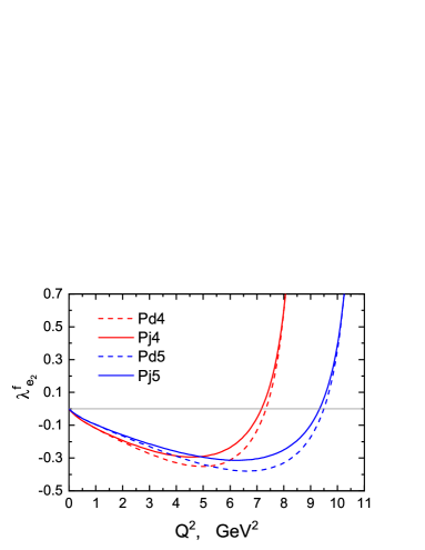
Figure 2: $Q^{2}$-dependence of the longitudinal polarization degree of the scattered electron $\lambda_{e_{2}}^{f}$ (31) at electron beam energies in the experiment Liyanage2020 . The lines $Pd4$, $Pd5$ (dashed) and $Pj4$, $Pj5$ (solid) correspond to the ratio $R=R_{d}$ in the case of dipole dependence and parametrization $R=R_{j}$ (39) from the paper Qattan2015 . The lines $Pd4$, $Pj4$ ($Pd5$, $Pj5$) correspond to the energies $E_{1}=4.725$ ($5.895$) GeV.

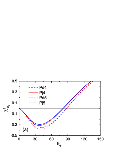
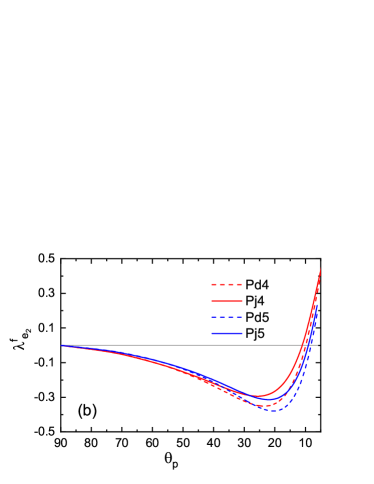
Figure 3: Angular dependence of the longitudinal polarization degree of the scattered electron $\lambda_{e_{2}}^{f}$ (31) at electron beam energies in the experiment Liyanage2020 . Panels (a) and (b) correspond to $\theta_{e}$-and $\theta_{p}$-dependencies expressed in degrees. The marking of lines $Pd4$, $Pd5$, $Pj4$, $Pj5$ is the same as in Figure 2.

As can be seen from Figure 2, the function $\lambda_{e_{2}}^{f}(Q^{2})$ (31) takes negative values for most of the allowed values and has a minimum for some of them. On a smaller part of the allowed values adjacent to $Q^{2}_{max}$ and amounting to approximately 9% of $Q^{2}_{max}$, it takes on positive values. At the boundary of the spectrum at $Q^{2}=Q^{2}_{max}$, the polarization transferred to the electron is equal to the polarization of the proton target, $\lambda_{e_{2}}^{f}(Q^{2}_{max})=P_{t}=0.70$.

Table 2: The degree of longitudinal polarization of the scattered electron $\lambda_{e_{2}}^{f}$ (31) at electron beam energies $E_{1}=4.725$ and $5.895\leavevmode\nobreak\ \mbox{GeV}$ and two values $Q^{2}=2.06$ and $5.66\leavevmode\nobreak\ \mbox{GeV}^{2}$ in the experiment Liyanage2020 . The values in the columns for $P_{d}$, $P_{j}$, $P_{k}$ correspond to the polarization transferred to the electron $\lambda_{e_{2}}^{f}$ (31) with dipole dependence, the parametrization (39) of Qattan Qattan2015 and Kelly Kelly2004 . The corresponding electron and proton scattering angles (in degrees) are given in columns for $\theta_{e}$ and $\theta_{p}$.

$E_{1}$, GeV	$Q^{2}$, $\mbox{GeV}^{2}$	$\theta_{e}\,(^{\circ})$	$\theta_{p}\,(^{\circ})$	$P_{d}$	$P_{j}$	$P_{k}$	$\Delta_{dj}$, %	$\Delta_{jk}$, %
5.895	2.06	15.51	45.23	–0.170	–0.163	–0.163	4.1	0.0
5.895	5.66	33.57	24.48	–0.363	–0.309	–0.308	14.9	0.3
4.725	2.06	19.97	43.27	–0.207	–0.197	–0.197	4.8	0,0
4.725	5.66	49.50	19.77	–0.336	–0.263	–0.262	21.7	0.6

Figure 3 shows the angular dependence of the transferred to the electron polarization $\lambda_{e_{2}}^{f}$ (31) in the $e\vec{p}\to\vec{e}p$ process at electron beam energies $4.725$ and $5.895\leavevmode\nobreak\ \mbox{GeV}$ in the experiment Liyanage2020 . The degree of polarization of the proton target was taken the same for all lines: $P_{t}=0.70$. Panels (a) and (b) correspond to the dependence on the scattering angles of the electron ($\theta_{e}$) and proton ($\theta_{p}$), expressed in degrees.

The parametrizations of Qattan Qattan2015 and Kelly Kelly2004 allow us to calculate the relative difference $\Delta_{dj}$ between the polarization effects in the $e\vec{p}\to\vec{e}p$ process in the case of conservation and violation of the SFF scaling, as well as in the effects between these parametrizations $\Delta_{jk}$:

$$\Delta_{dj}=\Big{|}\frac{\rm{Pd}-\rm{Pj}}{\rm{Pd}}\Big{|},\;\Delta_{jk}=\Big{|}\frac{\rm{Pj}-\rm{Pk}}{\rm{Pj}}\Big{|},$$ (40)

where $P_{d}$, $P_{j}$ and $P_{k}$ are the polarizations calculated by formula (31) for $\lambda_{e_{2}}^{f}$ when using the corresponding parametrizations $R_{d}$, $R_{j}$ and $R_{k}$. The results of calculations of $\Delta_{dj}$ at electron beam energies of $4.725$ and $5.895\leavevmode\nobreak\ \mbox{GeV}$ are shown in Figure 4.

It follows from the graphs in Figure 4 that the relative difference between the polarization transferred from the initial proton to the final electron in the $e\vec{p}\to\vec{e}p$ process in the case of conserving and violation of the scaling of the SFF can reach 70%, which can be used to set up a polarization experiment by measuring the ratio $R$.

Numerical values of the polarization transferred to the final electron in the $e\vec{p}\to\vec{e}p$ process for the three considered parametrizations of the ratio $R$ at $E_{1}$ and $Q^{2}$ used in the experiment Liyanage2020 , are presented in Table 2. In it, the columns of values $P_{d}$, $P_{j}$ and $P_{k}$ correspond to the dipole dependence $R_{d}$, parametrizations $R_{j}$ (39) and $R_{k}$ Kelly2004 ; columns $\Delta_{dj}$, $\Delta_{jk}$ correspond to the relative difference (40) (expressed in percent) at electron beam energies of $4.725$ and $5.895\leavevmode\nobreak\ \mbox{GeV}$ and two values of $Q^{2}$ equal to $2.06$ and $5.66\leavevmode\nobreak\ \mbox{GeV}^{2}$. It follows from Table 2 that the relative difference between $Pj5$ and $Pd5$ at $Q^{2}=2.06\leavevmode\nobreak\ \mbox{GeV}^{2}$ is 4.1% and between $Pj4$ and $Pd4$ it is 4.8%. At $Q^{2}=5.66\leavevmode\nobreak\ \mbox{GeV}^{2}$, the difference increases and becomes equal to 14.9 and 21.7%, respectively. Note that the relative difference $\Delta_{jk}$ between $P_{j}$ and $P_{k}$ for all $E_{1}$ and $Q^{2}$ in Table 2 is less than 1%.

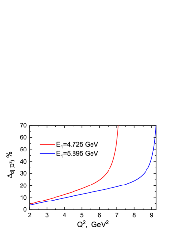
Figure 4: $Q^{2}$-dependence of the relative difference $\Delta_{dj}$ (40) at electron beam energies $E_{1}=4.725\leavevmode\nobreak\ \mbox{GeV}$ (red line) and $E_{1}=5.895\leavevmode\nobreak\ \mbox{GeV}$ (blue line). For all lines, the degree of polarization of the proton target was taken to be the same $P_{t}=0.70$.

Conclusion.—In this paper, we have considered a possible method for measuring the ratio $R\equiv\mu_{p}G_{E}/G_{M}$ based on the transfer of polarization from the initial proton to the final electron in the $e\vec{p}\to\vec{e}p$ process, in the case when their spins are parallel, i.e. when an electron is scattered in the direction of the spin quantization axis of the resting proton target. For this purpose, in the kinematics of the SANE collaboration experiment Liyanage2020 , using the parametrizations of Qattan Qattan2015 and Kelly Kelly2004 , a numerical analysis was carried out of the dependence of the degree of polarization of the scattered electron on the square of the momentum transferred to the proton, as well as from the scattering angles of the electron and proton. As it turned out, the parametrizations of Qattan Qattan2015 and Kelly Kelly2004 give almost identical results in calculations. It is established that the difference in the degree of longitudinal polarization of the final electron in the case of conservation and violation of the SFF scaling can reach 70 %, which can be used to conduct a new type of polarization experiment to measure the ratio $R$.

At present, an experiment to measure the longitudinal polarization degree transferred to an unpolarized electron in the $e\vec{p}\to\vec{e}p$ process when it is scattered in the direction of the spin quantization axis of a resting proton seems quite real since a proton target with a high degree of polarization $P_{t}=70\pm 5$ % was created in principle and has already been used in the experiment Liyanage2020 . For this reason, it would be most appropriate to conduct the proposed experiment at the setup used in Liyanage2020 at the same $P_{t}=0.70$, electron beam energies $E_{1}=4.725$ and $5.895\leavevmode\nobreak\ \mbox{GeV}$. The difference between conducting the proposed experiment and the one in Liyanage2020 consists in the fact that an incident electron beam must be unpolarized, and the detected scattered electron must move strictly along the direction of the spin quantization axis of the proton target. In the proposed experiment, it is necessary to measure only the longitudinal polarization degree of the scattered electron, which is an advantage compared to the method Rekalo74 used in JLab-experiments.

Acknowledgements.—This work was carried out within the framework of scientific cooperation Belarus-JINR and State Program of Scientific Research “Convergence-2025” of the Republic of Belarus under Projects No. 20221590 and No. 20210852.