Anatomy of linear and non-linear intermolecular exchange in $S=1$ nanographenes

Abstract

Nanographene triangulenes with a $S=1$ ground state have been used as building blocks of antiferromagnetic Haldane spin chains realizing a symmetry protected topological phase. By means of inelastic electron spectroscopy, it was found that the intermolecular exchange contains both linear and non-linear interactions, realizing the bilinear-biquadratic Hamiltonian. Starting from a Hubbard model, and mapping it to an interacting Creutz ladder, we analytically derive these effective spin-interactions using perturbation theory, up to fourth order. We find that for chains with more than two units other interactions arise, with same order-of-magnitude strength, that entail second neighbor linear, and three-site non-linear exchange. Our analytical expressions compare well with experimental and numerical results. We discuss the extension to general $S=1$ molecules, and give numerical results for the strength of the non-linear exchange for several nanographenes. Our results pave the way towards rational design of spin Hamiltonians for nanographene based spin chains.

Non-linear exchange, i.e., spin interactions that go beyond the simple Heisenberg coupling between two spins, play a prominent role in many physical systems, such as antiferromagnetic transition metal oxides[1], magnetic impurities in insulators[2], magnetic multilayers[3], chiral magnets[4] and magnetic two-dimensional materials[5]. Non-linear exchange is a key ingredient in the exactly solvable AKLT models[6], whose ground state is a resource for measurement based quantum computing[7].

The relative size and sign of linear and non-linear exchange can have a dramatic impact in several contexts. For instance, whereas the swap gate, or permutation operator, for spin qubits can be implemented with a linear Heisenberg interaction[8], for spin qudits it requires the presence of non-linear exchange terms[9]. Alternatively, in the case of the two-dimensional $S=3/2$ honeycomb lattice, the relative size of linear and non-linear exchange controls the nature of the ground state and its excitation spectrum [6, 10, 11].

Here we undertake the exploration of non-linear exchange in $S=1$ nanographenes. This class of system features outstanding flexibility to realize $S=1$ molecules with different shapes and sizes. It has been recently shown[12] that there are 383 different nanographenes that can be formed with 9 hexagons or less. Therefore, this type of system provides an ideal arena to engineer intermolecular exchange. One of the simplest $S=1$ nanographenes is the so-called [3]-triangulene.

Triangulenes are graphene fragments with the shape of an equilateral triangle, of various sizes and terminated with zigzag edges; these are customarily defined in terms of the number of benzenes, $n$, in a given edge[13, 14] (termed a [n]-triangulene). Based on Lieb’s theorem for the Hubbard model for bipartite lattices at half-filling [15], $[n]$-triangulenes are predicted to be open-shell multiradicals, with the spin of the ground state scaling as $2S=n-1$, associated with a half-full shell of $n-1$ in-gap non-bonding zero modes[16, 13, 17, 18, 19, 20].

Due to recent breakthroughs in bottom-up synthesis techniques [21, 22, 23, 24, 25], and the capability of atomic precision manipulation of organic molecules, triangulenes have been used as building blocks of larger molecular structures [26, 27, 28, 29]. A prime example of this is the recent realization of Haldane spin chains, where [3]-triangulenes (henceforth referred simply as triangulene) were coupled in order to generate chains with more than 16 units [27]. There, the inelastic electron tunneling spectroscopy (IETS) was described with an effective $S=1$ spin Hamiltonian that included both linear and non-linear exchange terms, i.e. the so called BLBQ Hamiltonian [30, 31, 32, 33, 34]:

$$H_{\text{BLBQ}}=\sum_{i}J\boldsymbol{S}_{i}\cdot\boldsymbol{S}_{i+1}+B\left(\boldsymbol{S}_{i}\cdot\boldsymbol{S}_{i+1}\right)^{2},$$ (1)

where each triangulene is represented by a spin-1 operator $\boldsymbol{S}_{i}$, the sum runs over all triangulenes in the chain and the parameters $J$ and $B$ are the linear and non-linear exchange couplings, respectively. The introduction of the non-linear exchange term proved essential to increase the accuracy of the spin model when compared with experimental data [27] and full fermionic numerical approaches [32].

In the following, we derive the effective $S=1$ spin Hamiltonian (1) starting from a fermionic model for the nanographenes. Importantly, our derivation unveils the presence of additional second neighbor linear interactions, and non-linear exchange that involve three-spin terms, with strength comparable to $B$ in Eq. (1). As a fermionic model we use a single-orbital Hubbard model (see Supporting Information), containing hoppings between first ($t$) and third neighbor ($t_{3}$) sites, and an on-site Hubbard repulsion term ($U$) which deals with the intra-atomic Coulomb repulsion cost associated with having a given $\pi$-orbital doubly occupied [20]. The Hubbard model has been validated by comparison with multiconfigurational calculations obtained with full-quantum chemistry ab-initio methods [20], for $t=-2.7$ eV, $t_{3}\sim t/10$ and $U\sim|t|$ [35].

As a starting point, we employ a Hubbard Hamiltonian at half-filling to describe the smallest chain, i.e. a triangulene dimer. In order to derive the effective spin model, we describe the fermionic many-body states of the nanographenes in a truncated Hilbert space, corresponding to the complete active space (CAS) approximation (see Supporting Information) [20, 27, 36, 37]. In Fig. 1 (a) and (b) we show the single-particle energies for the triangulene dimer with $t_{3}=t/10$ and $t_{3}=0$; in both cases two possible choices of active spaces are indicated. When $t_{3}=0$ one finds four states with zero energy; these correspond to the unhybridized zero modes of the individual triangulenes. For $t_{3}=t/10$, intermolecular hybridization promoted by $t_{3}$ lifts this degeneracy. In panels (c) and (d) of the same figure, the absolute value of the site representation of the four modes closest to zero energy are depicted for $t_{3}=t/10$ and $t_{3}=0$. For the latter case, the wave functions were chosen as eigenfunctions of the $C_{3}$ symmetry operator with eigenvalues $\pm 2\pi/3$. For future reference, we refer to panel (c) as the molecular orbital basis, and to panel (d) as the $C_{3}$ symmetric basis.

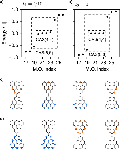
Figure 1: Single particle energies for the triangulene dimer with $t_{3}=t/10$ (a) and $t_{3}=0$ (b). Energies are given in unit of $|t|=2.7$ eV. The dashed boxes indicate two possible choices for the active space where the Hubbard Hamiltonian is represented. CAS($N_{O},N_{e}$) refers to an active space with $N_{O}$ modes where $N_{e}$ electrons are distributed). Panels (c) and (d) show the absolute value of the site representation of the four molecular orbitals closer to zero energy for $t_{3}=t/10$ and $t_{3}=0$, respectively. Each circle is colored according to the sublattice where it is located.

To gain physical insight about the properties of this system, we represent the Hamiltonian in the $C_{3}$ symmetric basis taking into account only the four modes at zero energy. The representation of the Hubbard model in that basis leads to the following effective Hamiltonian:

$$H =\sum_{\mu^{\prime}\mu}\sum_{\sigma}\tau_{\mu^{\prime}\mu}d^{\dagger}_{\mu^{\prime},\sigma}d_{\mu,\sigma}+\sum_{\mu}\mathcal{U_{\mu}}n_{\mu,\uparrow}n_{\mu,\downarrow}$$

$$+\sum_{\triangle}\mathcal{J}_{\triangle_{+},\triangle_{-}}\left(n_{\triangle_{+},\uparrow}n_{\triangle_{-},\downarrow}+n_{\triangle_{-},\uparrow}n_{\triangle_{+},\downarrow}\right)$$

$$+\sum_{\triangle}\mathcal{J}_{\triangle_{+},\triangle_{-}}\left(d^{\dagger}_{\triangle_{+},\uparrow}d_{\triangle_{-},\uparrow}d^{\dagger}_{\triangle_{-},\downarrow}d_{\triangle_{+},\downarrow}+\text{h.c.}\right)$$ (2)

where $\mu$ and $\mu^{\prime}$ run over the four $C_{3}$ symmetric modes and $\sigma=\uparrow,\downarrow$. The sums over $\triangle$ run over the two triangulenes, and $\triangle_{\pm}$ refers to the modes with eigenvalues $\pm 2\pi/3$ in a given triangulene. The operator $d^{(\dagger)}_{\mu,\sigma}$ annihilates (creates) an electron in the $\mu$ mode with spin $\sigma$, and $n_{\mu,\sigma}=d^{\dagger}_{\mu,\sigma}d_{\mu,\sigma}$.

This Hamiltonian contains three distinct types of terms. The first term in Eq. (2) represents the hopping between two modes, $\mu$ and $\mu^{\prime}$, with an amplitude $\tau_{\mu\mu^{\prime}}=t_{3}\sum_{\langle\langle\langle i,j\rangle\rangle\rangle}\Phi^{*}_{\mu}(i)\Phi_{\mu^{\prime}}(j)$ where $\Phi_{\mu}(i)$ is the site representation of the $\mu$-mode (depicted in Fig. 1). This hopping amplitude is zero when the two modes are localized in the same sublattice; thus, hoppings between modes in the same triangulene vanish. In addition, due to the $C_{3}$ symmetry of the $\mu$-modes, all the finite hoppings have the same absolute value, which we label simply as $\tau$. The pictorial representation of this hopping structure, shown in fig. 2, reveals the single-particle Hamiltonian maps into a Creutz ladder model[38] with vanishing vertical hoppings.

The remaining terms in the Hamiltonian account for electron-electron interactions. The second term of Eq. (2), corresponds to an effective Hubbard repulsion that penalizes the double occupancy of a given mode $\mu$, with the energy penalty being proportional to the inverse participation ratio (IPR), and is defined as $\mathcal{U}_{\mu}=U\sum_{i}|\Phi_{\mu}(i)|^{4}$, where the sum runs over all the sites. Again, due to the $C_{3}$ symmetry of the modes, one finds $\mathcal{U}_{\mu}\equiv\mathcal{U}$ is independent of $\mu$.

The last two lines in Eq. (2) describe an intra-triangulene ferromagnetic exchange interaction, with the exchange coupling given by $\mathcal{J}_{\mu\mu^{\prime}}=U\sum_{i}|\Phi_{\mu}(i)|^{2}|\Phi_{\mu^{\prime}}(i)|^{2}$. As before, $\mathcal{J}_{\mu\mu^{\prime}}=\mathcal{J}$ is independent of $\mu$ and $\mu^{\prime}$, and $\mathcal{U}=\mathcal{J}$.

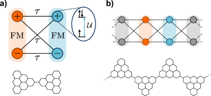
Figure 2: (a) Schematic representation of the interactions present in the Hamiltonian of Eq. (2), with modes in the same triangulene ferromagnetically coupled, and hoppings between the two triangulenes; (b) Extension of the model for the case of a triangulene chain.

Therefore the model (2) realizes a Creutz-ladder [38], with the difference that the vertical hoppings are replaced by a ferromagnetic exchange and there are Hubbard interactions. In Fig. 2 we present a pictorial representation of the Hamiltonian of Eq. (2) for the triangulene dimer, as well as the extension to larger structures, e.g. a triangulene chain. The extension of Eq. (2) to triangulene chains is easily obtained by running the sums over all triangulenes (see Supporting Information for the numerical solution of Eq.(2) for a triangulene dimer and trimer).

Let us note in passing, that for molecules less symmetric than triangulenes, for example panels (c) to (f) of Fig. 4, the hoppings $\tau_{\mu\mu^{\prime}}$, the effective Hubbard repulsion $\mathcal{U}_{\mu}$, and the exchange coupling $\mathcal{J}_{\mu\mu^{\prime}}$ are in principle mode-dependent. Moreover, it might be necessary to include a new term associated with electron-pair hoppings in Eq. (2). As discussed in [20], this term vanishes for triangulenes, but may be finite for other molecules. Including it is straightforward, and does not affect the main physical features we presently wish to discuss.

Starting from the many-body fermionic model just presented, we now produce an effective low energy description which can be related to the effective BLBQ spin model. To this end, we shall employ degenerate perturbation up to fourth order, treating the hoppings $\tau$ as a perturbation.

For the unperturbed system ($\tau=0$) the two pairs of modes are decoupled, and each triangulene can be studied individually. At half-filling, with two electrons per triangulene, the lowest energy states in a given triangulene are $|\uparrow\rangle|\uparrow\rangle$, $|\downarrow\rangle|\downarrow\rangle$ and $\left(|\uparrow\rangle|\downarrow\rangle+|\downarrow\rangle|\uparrow\rangle\right)/\sqrt{2}$, where each ket refers to one of the $C_{3}$ symmetric modes in a triangulene. These states correspond to the three spin projections of a $S=1$ state formed by the ferromagnetic coupling of two spin-1/2 electrons, i.e. $|\uparrow\rangle|\uparrow\rangle\equiv|\Uparrow\rangle$, $|\downarrow\rangle|\downarrow\rangle\equiv|\Downarrow\rangle$ and $\left(|\uparrow\rangle|\downarrow\rangle+|\downarrow\rangle|\uparrow\rangle\right)/\sqrt{2}\equiv|+\rangle$, with the ket on the right hand side referring to the state of the triangulene as a whole. With these three states in each triangulene, the total unperturbed dimer Hamiltonian at half-filling is nine-fold degenerate.

Representing Eq. (1) in the basis of two spin-1 objects, and focusing on the $S_{z}=0$ sector, one finds that while the bilinear term, proportional to $J$, is responsible for connecting the state $|+\rangle|+\rangle$ with the states $|\Uparrow\rangle|\Downarrow\rangle$ and $|\Downarrow\rangle|\Uparrow\rangle$, the biquadratic term, proportional to $B$, unlocks a new interaction between the states $|\Uparrow\rangle|\Downarrow\rangle$ and $|\Downarrow\rangle|\Uparrow\rangle$. Recalling the definition of the spin-1 states in terms of two spin-1/2, one realizes that while the processes mediated by $J$ link states which differ by two spin flips, the process mediated by $B$ connects states differing by four spin flips. Hence, the biquadratic interaction is only to be expected in 4th order perturbation theory, while the bilinear term should already be present in 2nd order.

The expressions for the 2nd and 4th order corrections in degenerate perturbation theory read [39, 40]:

$$h^{(2)}_{kp} =\sum_{m}\frac{\langle k|H_{\tau}|m\rangle\langle m|H_{\tau}|p\rangle}{\Delta E^{(0)}_{m}}$$ (3)

$$h^{(4)}_{kp} =\sum_{mm^{\prime}m^{\prime\prime}}\frac{\langle k|H_{\tau}|m\rangle\langle m|H_{\tau}|m^{\prime}\rangle\langle m^{\prime}|H_{\tau}|m^{\prime\prime}\rangle\langle m^{\prime\prime}|H_{\tau}|p\rangle}{\Delta E^{(0)}_{m}\Delta E^{(0)}_{m^{\prime}}\Delta E^{(0)}_{m^{\prime\prime}}}$$

$$-\sum_{mm^{\prime}l}\frac{\langle k|H_{\tau}|m\rangle\langle m|H_{\tau}|l\rangle\langle l|H_{\tau}|m^{\prime}\rangle\langle m^{\prime}|H_{\tau}|p\rangle}{\Delta E^{(0)}_{m}\Delta E^{(0)}_{m}\Delta E^{(0)}_{m^{\prime}}}$$ (4)

where $k$, $p$ and $l$ label states inside the degenerate ground state, and the sums run over all the states outside that subspace. The perturbation is $H_{\tau}=\sum_{\mu\mu^{\prime}}\sum_{\sigma}\tau_{\mu\mu^{\prime}}d^{\dagger}_{\mu\sigma}d_{\mu\sigma}$ and $\Delta E^{(0)}_{m}$ is the unperturbed energy of the $|m\rangle$ state relative to the ground state. In the absence of applied magnetic field, the odd-order corrections vanish identically [41]. One important aspect to note is that even though the initial and final state correspond to open-shell configurations with two electrons per triangulene, the intermediate states contain closed-shell configurations, as well as charge excitations, with different number of electrons in the two triangulenes.

In 2nd order perturbation theory, where only two electron flips are considered, a finite contribution for $J$ is found, which for the present system simply reads $J^{(2)}=2\tau^{2}/\mathcal{U}$ (see Supporting Information). This result is similar to the one usually found when when a Hubbard chain is mapped to a Heisenberg chain of antiferromagnetically coupled spins; the different numerical pre-factor steming from the different geometry of our system.

Progressing to 4th order perturbation theory, where processes involving up to four electron are considered, different paths appear which allow for $|\Uparrow\rangle|\Downarrow\rangle\rightarrow|\Downarrow\rangle|\Uparrow\rangle$. Carrying out the necessary calculations, one finds that finite contributions appear for both $J$ and $B$. These are given by $J^{(4)}=4\tau^{4}/\mathcal{U}^{3}$ and $B^{(4)}=8\tau^{4}/\mathcal{U}^{3}$. The 2nd order contribution to $J$ dominates its 4th order counterpart in the physically relevant region of the parameter space, and $J^{(4)}$ may be neglected. Hence, combining the results from second and forth order perturbation theory, we find in leading order:

$$J\approx\frac{2\tau^{2}}{\mathcal{U}},\quad B\approx\frac{8\tau^{4}}{\mathcal{U}^{3}},\quad\beta\equiv\frac{B}{J}\approx\frac{4\tau^{2}}{\mathcal{U}^{2}}.$$ (5)

Using the definitions of $\tau$ [35] and $\mathcal{U}$ [20], and assuming $t_{3}\approx t/10$, one can estimate the strength of the quadratic exchange with respect to the linear one, characterized by $\beta$, using $\beta\approx 0.1(t/U)^{2}$. This rough approximation yields a nice agreement with the value $\beta=0.09$ that was found in the description of experimental data in [27]. This good agreement, together with the analytical expressions of Eq. (5), indicate that non-linear exchange is a higher-order manifestation of the same underlying kinetic exchange mechanism[1] that gives rise to linear exchange.

To validate our analytical expressions we shall now compare them with the results found from numerical diagonalization. The numerical results are obtained by first diagonalizing Eq. (2), followed by matching the energies of the first excitations with those of the BLBQ Hamiltonian (see Supporting Information for details). This gives numerically both $J$ and $B$ as a function of the parameters of the microscopic model, $U$ and $t_{3}$, and allows the comparison with Eq. (5).

In Fig. 3 we show the comparison between the analytical expressions found for $J$ and $B$ and the numerical results.

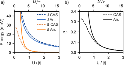
Figure 3: Comparison between the analytical expression and the result found from numerical diagonalization for (a) the linear exchange $J$ and the non-linear exchange $B$, and (b) the ratio $\beta=B/J$ as a function of the on-site Hubbard repulsion $U$ in units of $|t|=2.7$ eV with $t_{3}=t/10$.

Inspecting this figure reveals an excellent agreement between the two approaches, especially in the region $U\gg|t|$ where perturbation theory is valid. Crucially, this agreement holds near $U\sim|t|$, the physically relevant region. For $U=|t|$, one finds the linear exchange $J=20$ meV and $\beta=0.11$. As $U$ increases $\beta$ approaches 0, and a Heisenberg-like picture is recovered. For $U<<|t|$, outside the validity region of perturbation theory, the mapping to a spin model fails since the order of low energy excitations is no longer the same in the two approaches. The fact that $\beta$ is bounded by the AKLT limit $\beta=1/3$ is a consequence of Lieb’s theorem, which prevents a four-fold degenerate ground state.

Having completed the study of the triangulene dimer, we extend our analysis to larger chains. Generalizing Eq. (2) to include more triangulenes, and once again employing perturbation theory up to 4th order, we find that for a chain composed of $N$ triangulenes the effective spin Hamiltonian reads (see Supporting Information for detailed derivation):

$$H_{N} =J\sum_{i=1}^{N-1}\boldsymbol{S}_{i}\cdot\boldsymbol{S}_{i+1}+B\sum_{i=1}^{N-1}(\boldsymbol{S}_{i}\cdot\boldsymbol{S}_{i+1})^{2}$$

$$+J_{2}\sum_{i=1}^{N-2}\boldsymbol{S}_{i}\cdot\boldsymbol{S}_{i+2}$$

$$+B_{1,1}\sum_{i=1}^{N-2}(\boldsymbol{S}_{i}\cdot\boldsymbol{S}_{i+1})(\boldsymbol{S}_{i+1}\cdot\boldsymbol{S}_{i+2})+\text{h.c.}.$$ (6)

While the first line corresponds to the BLBQ model for $N$ triangulenes, the second and third lines contain new exchange interactions; the former describes an antiferromagnetic second neighbor linear exchange, and the latter a ferromagnetic quadratic exchange involving two adjacent triangulene pairs. We note that the antiferromagnetic second neighbor linear exchange might promote frustration if its strength becomes comparable with $J$. If perturbation theory is extended up to sixth or eight order, additional exchange interactions appear; however, since these are in higher order of $\tau/\mathcal{U}$ we neglect their contribution. Crucially, the terms proportional to $J_{2}$ and $B_{1,1}$ appear in the same order of perturbation theory as $B$ and therefore must be accounted for. To leading order, we find:

$$J=\frac{2\tau^{2}}{\mathcal{U}},B=\frac{8\tau^{4}}{\mathcal{U}^{3}},J_{2}=\frac{79\tau^{4}}{12\mathcal{U}^{3}},B_{1,1}=-\frac{37\tau^{4}}{12\mathcal{U}^{3}}$$ (7)

Hence, a consistent description of triangulene spin chains should include this terms, missing in previous analysis[27].

We now briefly explore the non-linear exchange of various $S=1$ dimers. By applying numerical diagonalization in the minimal CAS, and comparing it with the excitation energies of the BLBQ Hamiltonian, we obtain the value of $\beta$ for different dimers composed of molecules with a triplet ground state. This should predict the relevance of non-linear exchange, as well as its tunability, in chains formed with different building blocks. In Fig. 4 (b) we show a triangulene dimer, where a benzene is introduced in the middle. Formally, this molecule is nearly identical to the dimer we considered in the text (depicted in panel (a)), with the main difference being that due to the extra benzene, intermolecular hybridization between the two triangulenes is greatly diminished, resulting in a smaller $\tau$. This leads to $\beta=0.002$, two orders of magnitude smaller than what we found for the case without the spacer (see Supporting Information for details on the change in this value due to a larger active space). Next, we consider the molecule of panel (c), where each monomer is composed of two Phenalenyl side-by-side; for this dimer $\beta=0.14$. As benzenes are added between the two Phenalenyl, depicted in panels (d) [42] and (e), the value of $\beta$ increases to $\beta=0.16$ and $\beta=0.18$, respectively. This increase in $\beta$ may be ascribed to the decrease of the IPR of the zero modes of the individual molecules. At last, we consider panel (f), where an additional benzene is added close to the binding site of the two molecules. This leads to a significant decrease of $\beta$ to $\beta=0.03$. The reason for this sharp decrease is similar to the one we gave when discussing panel (b). Hence, we see that by carefully choosing the geometry of the molecules used as building blocks, it should be possible to engineer the strength of non-linear exchange.

Figure 4: Values obtained for $\beta=B/J$ by numerically diagonalizing the Hubbard Hamiltonian in a restricted Hilbert space with 4 modes only, for dimers obtained from $S=1$ building blocks, taking $U=|t|$, $t_{3}=t/10$ and $|t|=2.7$eV.

Even though we restricted our analysis to the minimal CAS, accounting only for the zero modes, additional orbitals could have been included in the calculation (see Fig. 1). This would introduce the so-called Coulomb driven super-exchange discussed in [37]. We have verified that including this additional mechanism would slightly change the numerical results, but preserve the qualitative features of the model.

Conclusions: We have considered chains of $S=1$ nanographenes, taking the case of triangulene chains as the prototypical example. Using perturbation theory we have found that non-linear exchange interactions are a higher-order manifestation of the same mechanisms that give rise to linear exchange, and we have obtained analytical expressions for their amplitude. The analytical results permit us to relate molecule geometry with $\beta$, the degree of exchange non-linearity. In addition, our analysis with more than two molecules shows that new terms appear in the Hamiltonian, namely a second neighbor linear and a three-site non linear exchange interaction, going beyond the BLBQ paradigm. Future work will address the impact of these extra terms on the well established phase diagram of the BLBQ model.

We acknowledge fruitful discussions with Gonçalo Catarina, António Costa and David Jacob. We acknowledge financial support from FCT (Grant No. PTDC/FIS-MAC/2045/2021), SNF Sinergia (Grant Pimag), FEDER /Junta de Andalucía, (Grant No. P18-FR-4834), Generalitat Valenciana funding Prometeo2021/017 and MFA/2022/045, and funding from MICIIN-Spain (Grant No. PID2019-109539GB-C41).

References

- Anderson [1959] P. W. Anderson, Physical Review 115, 2 (1959).
- Harris and Owen [1963] E. Harris and J. Owen, Physical review letters 11, 9 (1963).
- Slonczewski [1991] J. Slonczewski, Physical Review Letters 67, 3172 (1991).
- Paul et al. [2020] S. Paul, S. Haldar, S. Von Malottki, and S. Heinze, Nature communications 11, 4756 (2020).
- Kartsev et al. [2020] A. Kartsev, M. Augustin, R. F. Evans, K. S. Novoselov, and E. J. Santos, npj Computational Materials 6, 150 (2020).
- Affleck et al. [1987] I. Affleck, T. Kennedy, E. H. Lieb, and H. Tasaki, Phys. Rev. Lett. 59, 799 (1987).
- Wei et al. [2011] T.-C. Wei, I. Affleck, and R. Raussendorf, Phys. Rev. Lett. 106, 070501 (2011).
- DiVincenzo et al. [2000] D. P. DiVincenzo, D. Bacon, J. Kempe, G. Burkard, and K. B. Whaley, nature 408, 339 (2000).
- Segraves [1964] P. H. Segraves, Representation of Permutation Operator in Quantum Mechanics, Master’s thesis, University of British Columbia (1964).
- Pomata and Wei [2020] N. Pomata and T.-C. Wei, Phys. Rev. Lett. 124, 177203 (2020).
- Ganesh et al. [2011] R. Ganesh, D. Sheng, Y.-J. Kim, and A. Paramekanti, Physical Review B 83, 144414 (2011).
- Yan et al. [2023] Y. Yan, F. Zheng, B. Qie, J. Lu, H. Jiang, Z. Zhu, and Q. Sun, The Journal of Physical Chemistry Letters 14, 3193 (2023).
- Fernández-Rossier and Palacios [2007] J. Fernández-Rossier and J. J. Palacios, Physical Review Letters 99, 177204 (2007).
- Su et al. [2020a] J. Su, M. Telychko, S. Song, and J. Lu, Angewandte Chemie International Edition 59, 7658 (2020a).
- Lieb [1989] E. H. Lieb, Physical review letters 62, 1201 (1989).
- Ovchinnikov [1978] A. A. Ovchinnikov, Theoretica Chimica Acta 47, 297 (1978).
- Wang et al. [2008] W. L. Wang, S. Meng, and E. Kaxiras, Nano letters 8, 241 (2008).
- Wang et al. [2009] W. L. Wang, O. V. Yazyev, S. Meng, and E. Kaxiras, Physical review letters 102, 157201 (2009).
- Yazyev [2010] O. V. Yazyev, Reports on Progress in Physics 73, 056501 (2010).
- Ortiz et al. [2019] R. Ortiz, R. Á. Boto, N. García-Martínez, J. C. Sancho-García, M. Melle-Franco, and J. Fernández-Rossier, Nano Lett. 19, 5991 (2019).
- Ruffieux et al. [2016] P. Ruffieux, S. Wang, B. Yang, C. Sánchez-Sánchez, J. Liu, T. Dienel, L. Talirz, P. Shinde, C. A. Pignedoli, D. Passerone, et al., Nature 531, 489 (2016).
- Mishra et al. [2019] S. Mishra, D. Beyer, K. Eimre, J. Liu, R. Berger, O. Groning, C. A. Pignedoli, K. Müllen, R. Fasel, X. Feng, et al., Journal of the American Chemical Society 141, 10621 (2019).
- Su et al. [2019] J. Su, M. Telychko, P. Hu, G. Macam, P. Mutombo, H. Zhang, Y. Bao, F. Cheng, Z.-Q. Huang, Z. Qiu, et al., Science advances 5, eaav7717 (2019).
- Su et al. [2020b] J. Su, M. Telychko, S. Song, and J. Lu, Angewandte Chemie International Edition 59, 7658 (2020b).
- Mishra et al. [2021a] S. Mishra, K. Xu, K. Eimre, H. Komber, J. Ma, C. A. Pignedoli, R. Fasel, X. Feng, and P. Ruffieux, Nanoscale 13, 1624 (2021a).
- Mishra et al. [2020] S. Mishra, D. Beyer, K. Eimre, R. Ortiz, J. Fernández-Rossier, R. Berger, O. Gröning, C. A. Pignedoli, R. Fasel, X. Feng, et al., Angewandte Chemie International Edition (2020).
- Mishra et al. [2021b] S. Mishra, G. Catarina, F. Wu, R. Ortiz, D. Jacob, K. Eimre, J. Ma, C. A. Pignedoli, X. Feng, P. Ruffieux, et al., Nature 598, 287 (2021b).
- Hieulle et al. [2021] J. Hieulle, S. Castro, N. Friedrich, A. Vegliante, F. R. Lara, S. Sanz, D. Rey, M. Corso, T. Frederiksen, J. I. Pascual, et al., Angewandte Chemie International Edition 60, 25224 (2021).
- Cheng et al. [2022] S. Cheng, Z. Xue, C. Li, Y. Liu, L. Xiang, Y. Ke, K. Yan, S. Wang, and P. Yu, Nature Communications 13, 1705 (2022).
- Tanaka et al. [2018] K. Tanaka, Y. Yokoyama, and C. Hotta, Journal of the Physical Society of Japan 87, 023702 (2018).
- Hu et al. [2020] W.-J. Hu, S.-S. Gong, H.-H. Lai, Q. Si, and E. Dagotto, Physical Review B 101, 014421 (2020).
- Catarina and Fernández-Rossier [2022] G. Catarina and J. Fernández-Rossier, Phys. Rev. B 105, L081116 (2022).
- Soni et al. [2022] R. Soni, N. Kaushal, C. Şen, F. A. Reboredo, A. Moreo, and E. Dagotto, New Journal of Physics 24, 073014 (2022).
- Catarina et al. [2023] G. Catarina, J. C. G. Henriques, A. Molina-Sánchez, A. T. Costa, and J. Fernández-Rossier, arXiv:2306.17153 (2023).
- Ortiz et al. [2022] R. Ortiz, G. Catarina, and J. Fernández-Rossier, 2D Materials 10, 015015 (2022).
- Jacob et al. [2021] D. Jacob, R. Ortiz, and J. Fernández-Rossier, Physical Review B 104, 075404 (2021).
- Jacob and Fernández-Rossier [2022] D. Jacob and J. Fernández-Rossier, Physical Review B 106, 205405 (2022).
- Creutz [1999] M. Creutz, Physical review letters 83, 2636 (1999).
- Calzado and Malrieu [2004] C. J. Calzado and J.-P. Malrieu, Physical Review B 69, 094435 (2004).
- Malrieu et al. [2014] J. P. Malrieu, R. Caballol, C. J. Calzado, C. De Graaf, and N. Guihery, Chemical reviews 114, 429 (2014).
- MacDonald et al. [1988] A. H. MacDonald, S. Girvin, and D. t. Yoshioka, Physical Review B 37, 9753 (1988).
- Su et al. [2020c] X. Su, C. Li, Q. Du, K. Tao, S. Wang, and P. Yu, Nano letters 20, 6859 (2020c).