The Schwinger effect by axial coupling in natural inflation model

Abstract

We investigate the process of the Schwinger effect by axial coupling in the natural single-field inflation model in two parts. First we consider the Schwinger effect when the conformal invariance of Maxwell action should be broken by axial coupling $I(\phi)F_{\mu\nu}\tilde{F}^{\mu\nu}$ with the inflaton field by identifying the standard horizon scale $k=aH$ at the very beginning of inflation for additional boundary term and use several values of coupling constant $\chi_{1}$ and estimate electric and magnetic energy densities and energy density of produced charged particles due to the Schwinger effect.We find that for both coupling functions the energy density of the produced charged particles due to the Schwinger effect is so high and spoils inflaton field.In fact the strong coupling or back-reaction occurs because the energy density of produced charged particles is exceeding of inflaton field.We use two coupling functions to break conformal invariance of maxwell action.The simplest coupling function $I\left(\phi\right)=\chi_{1}\frac{\phi}{M_{p}}$ and a curvature based coupling function $I\left(\phi\right)=12\chi_{1}e^{\left(\sqrt{\frac{2}{3}}\frac{\phi}{M_{p}}\right)}\left[\frac{1}{3M_{p}^{2}}\left(4V\left(\phi\right)\right)+\frac{\sqrt{2}}{\sqrt{3}M_{p}}\left(\frac{dV}{d\phi}\right)\right]$ where $V\left(\phi\right)$ is the potential of natural inflation. In second part , in oder to avoid strong back-reaction problem we identify the horizon scale $k_{H}=aH|\zeta|,\zeta=\frac{{I}^{\prime}\left(\phi\right)\dot{\phi}}{H}$ in which a given Fourier begins to become tachyonically unstable.The effect of this scale is reducing the value of coupling constant $\chi_{1}$ and weakening the back-reaction problem but in both cases strong coupling or strong back-reaction exists and the Schwinger effect is impossible. Therefore, the Schwinger effect in this model is not possible and spoils inflation.Instantly,the Schwinger effect produces very high energy density of charged particles which causes back-reaction problem and spoils inflaton field.We must stress that due to existence of strong back-reaction in two cases the energy density of the produced charged particles due to the Schwinger effect spoils inflaton field and we do not reach to the so-called conductivity of plasma.

I Introduction

We have recently shown in the natural single-field inflation model with kinetic coupling both magneto-genesis and the Schwinger effect exist.Kamarpour-Sobol:2018 ; Kamarpour:2023 .In Refs.Kronberg:1994 ; Grasso:2001 ; Widrow:2002 ; Giovannini:2004 ; Kandus:2011 ; Durrer:2013 ; Subramanian:2016 have been shown the strength of detected magnetic fields indicates a wide range,with values ranging from a few micogauss in galaxies and in cluster of galaxies to a very high as $10^{15}$ gauss in magnetars.Moreover,cosmic microwave background observations Planck:2015 ; Planck:2018 ; Sutton:2017 ; Jedamzik:2018 introduce upper and lower bounds.In addition,gamma rays emitted by distant blazars Neronov:2010 ; Tavecchio:2010 ; Taylor:2011 ; Caprini:2015 have shown the strength of large-scale magnetic fields $B_{0}$ ranging from $10^{-17}$ to $10^{-9}$ gauss.

In order to understand the origins of these magnetic fields , several investigations have been studied in literature such as the theory of structure formation through the astrophysical Biermann battery mechanism Biermann:1950 .In this mechanism , these fields are then amplified through various forms of dynamo and then spread into the intergalactic medium by outflows from galaxies. Zeldovich:1980book ; Lesch:1995 ; Kulsrud:1997 ; Colgate:2001 ; Rees:1987 ; Daly:1990 ; Ensslin:1997 ; Bertone:2006 .

Another theory implies that the origin of these fields is primordial and produced in early Universe Turner:1988 ; Ratra:1992 ; Hogan:1983 ; Quashnock:1989 ; Vachaspati:1991 .Among these theories ,it is thought that the most natural mechanism for the generation of large-coherence-scale magnetic fields would be inflation, a period of rapid expansion in the early Universe Turner:1988 .

In studies of early Universe many authors have indicated that during inflation ,quantum fluctuation of massless scalar and tensor fields can be amplified significantly which is thought to led to the formation of the large-scale structures observed in Universe todayMukhanov:1981 ; Hawking:1982 ; Starobinsky:1982 ; Guth:1982 ; Bardeen:1983 .In addition, it is thought that this amplification is responsible for the generation of relic gravitational waves Grishchuk:1975 ; Starobinsky:1979 ; Rubakov:1982 .

However,the conformal invariance of the Maxwell action does not allow of generation of any large-scaled magnetic fields Parker:1968 .Therefore, in this paper we break the conformal invariance by axial coupling interaction term of the form $I\left(\phi\right)F_{\mu\nu}\tilde{F}^{\mu\nu}$ Dolgov:1993 ; Gasperini:1995 ; Giovannini:2000 ; Atmjeet:2014 where $I\left(\phi\right)$ is a coupling function of the inflaton field $\phi$ and $F_{\mu\nu}=\partial_{\mu}A_{\nu}-\partial_{\nu}A_{\mu}$ is the electromagnetic field tensor and $\tilde{F}^{\mu\nu}=\frac{1}{2}\frac{\epsilon^{\mu\nu\rho\sigma}}{\sqrt{-g}}F_{\rho\sigma}$ .In this method , $\tilde{F}^{\mu\nu}$ does not depend on metric and does not contribute to the energy-momentum tensor.Because $F_{\mu\nu}\tilde{F}^{\mu\nu}=-4\textbf{E}\cdot\textbf{B}$ , the term $\textbf{E}\cdot\textbf{B}$ appears in our equations and should be approximated by simpler relation in order to solve system of equations. More importantly, due to axial coupling of inflaton field and electromagnetic field , the term $\textbf{E}\cdot\textbf{B}$ implies that the produced magnetic field is helical.Additionally, in axial coupling the electric energy density is almost equal to the magnetic energy density , i.e. $\rho_{E}\sim\rho_{B}$ Figueroa:2018 ; Notari:2016 ; Fujita:2015 ; Kamarpour:2021 ; Kamarpour:2022 ; Kamarpour:2023-I .Also, the conformal invariance can be broken by $I^{2}\left(\phi\right)F_{\mu\nu}F^{\mu\nu}$ which is called kinetic coupling, first introduced by Ratra Ratra:1992 and discussed in references Giovannini:2001 ; Bamba:2004 ; Martin:2008 ; Demozzi:2009 ; Kanno:2009 ; Ferreira:2013 ; Ferreira:2014 ; Vilchinskii:2017 .

In this paper we consider the Schwinger effect in natural inflation model by axial coupling only for strong field regime because for weak field the Schwinger effect is negligibleSobol-Gorbar:2021 .Briefly , the Schwinger effect is producing of charged particles from vacuum by strong electric field Schwinger:1951 .

Strong generated electric field is the result of coupling of the electromagnetic field and inflaton field. This effect has been studied in several papers.For instance, the case of a constant and homogeneous electric field in de Sitter space-time can be found in Refs. Afshordi:2014 ; Froeb:2014 ; Bavarsad:2016 ; Stahl:2016a ; Stahl:2016b ; Hayashinaka:2016a ; Hayashinaka:2016b ; Sharma:2017 ; Tangarife:2017 ; Hayashinaka:2018 ; Hayashinaka:thesis ; Stahl:2018 ; Geng:2018 ; Bavarsad:2018 .

It should be noted that,the cosmological Schwinger effect is consideration of expansion of the Universe and investigates the Schwinger effect in de Sitter space-time.In this case , expansion of the Universe is exponential.This effect drives some expressions for the production of charged particles by strong electric field.The interesting features of the cosmological Schwinger effect such as infrared hyper-conductivity in the bosonic with very small mass or massless particles have been studied in Refs.Afshordi:2014 ; Hayashinaka:2016a ; Hayashinaka:2016b ; Hayashinaka:2018 ; Hayashinaka:thesis ; Stahl:2018 .

However, the constant and homogeneous electric filed for the Schwinger effect contradicts the second law of thermodynamics because it would require the existence of ad hoc currents Giovannini:2018a . Instead, expressions for the Schwinger effect must be used in the case of a time-dependent electric field in the strong-field regime Kitamoto:2018 .

In this paper, we investigate the Schwinger effect by axial coupling in the natural inflation model with two coupling functions. The paper is organized as follows: we determine the model and find the solution for the background equations in the natural inflation model in Sect. II, where we also consider the axial coupling of the inflation field to the electromagnetic field with two coupling functions. We then obtain the mode-function and estimate the range of parameters for which the back-reaction problem does not occur for our model. In this part , we consider a system of self-consistent equations, including the Schwinger effect. Section III discusses the main idea of the Schwinger effect, including the Schwinger source term. In Sect. IV, we perform numerical calculations for both scenarios, when we use the standard horizon scale $k_{H}=aH$ and with the scale at which a given Fourier begins to become tachyonically unstable for two coupling functions and compare them. The summary of the obtained results is given in Sect. V.

II Natural inflation

We use the potential of the natural inflation model that was proposed in Refs. Freese:1990 ; Adams:1993 . For more details see our previous works in Refs. Kamarpour-Sobol:2018 ; Kamarpour:2023 .

$$V\left(\phi\right)=\Lambda^{4}\left[1-\cos\left(\frac{\phi}{f}\right)\right]$$ (1)

We consider a spatially flat Friedmann–Lemaître–Robertson–Walker(FLRW) Universe with metric tensor

$$g_{\mu\nu}={\rm diag}\,(1,\,-a^{2},\,-a^{2},\,-a^{2}),\quad\sqrt{-g}=a^{3},$$ (2)

and use the natural system of units where $\hbar=c=1$, $M_{p}=(8\pi G)^{-1/2}=2.4\cdot 10^{18}\,{\rm GeV}$ is a reduced Planck mass , and $e=\sqrt{4\pi\alpha}\approx 0.3$ is the absolute value of the electron’s charge.

II.1 Action

The action of the inflation field interacting with electromagnetic field by axial coupling reads

$$S=\int d^{4}x\sqrt{-g}\left[\frac{1}{2}\partial^{\mu}\phi\partial_{\mu}\phi-V(\phi)-\frac{1}{4}F_{\mu\nu}F^{\mu\nu}+\frac{1}{4}I\left(\phi\right)F_{\mu\nu}\tilde{F}^{\mu\nu}\right]$$ (3)

Variation for inflaton field $\phi$ reads

$$\frac{1}{\sqrt{-g}}\partial{{}_{\mu}}\left[\sqrt{-g}\partial{{}^{\mu}\phi}\right]+\frac{dV}{d\phi}=\frac{1}{4}\frac{dI\left(\phi\right)}{d\phi}F_{\mu\nu}\tilde{F}^{\mu\nu}$$ (4)

Also variation of gauge field $A_{\mu}$ gives following relation

$$\frac{1}{\sqrt{-g}}\partial_{\mu}\left[\sqrt{-g}I(\phi)\tilde{F}^{\mu\nu}-\sqrt{-g}F^{\mu\nu}\right]=0$$ (5)

In above equation $\tilde{F}^{\mu\nu}=\frac{1}{2}\frac{\epsilon^{\mu\nu\rho\sigma}}{\sqrt{-g}}F_{\rho\sigma}$ in which $\epsilon^{\mu\nu\rho\sigma}$ is the totally antisymmetric Levi-Civita symbol with $\epsilon^{0123}=1$.

Further manipulations of equation(5) gives following useful equation

$$\frac{1}{\sqrt{-g}}\partial_{\mu}\left[\sqrt{-g}{F}^{\mu\nu}\right]-I^{\prime}\left(\phi\right)\partial_{\mu}\phi\tilde{F}^{\mu\nu}=0$$ (6)

where $I^{\prime}\left(\phi\right)=\frac{dI\left(\phi\right)}{d\phi}$.Another useful equation is given by following relation

$$\frac{1}{\sqrt{-g}}\partial_{\mu}\left[\sqrt{-g}\tilde{F}^{\mu\nu}\right]=0$$ (7)

In Eq. (4) $F_{\mu\nu}\tilde{F}^{\mu\nu}=-4\textbf{E}\cdot\textbf{B}$ , by using this equation we obtain

$$\ddot{\phi}+3H\dot{\phi}+\frac{dV\left(\phi\right)}{d\phi}=-I^{\prime}\left(\phi\right)\textbf{E}\cdot\textbf{B}$$ (8)

In obtaining the above equation we assume homogeneous inflaton field $\phi=\phi\left(t\right)$.

Now, if we add a following gauge invariant Lagrangian $L_{charged}\left(A,\chi\right)$ to the action of equation 3

$$S_{gauge}=\int d^{4}x\sqrt{-g}L_{charged}\left(A,\chi\right),$$ (9)

then the total action will be given by following relation

$$S+S_{gauge}=\int d^{4}x\sqrt{-g}\left[\frac{1}{2}\partial^{\mu}\phi\partial_{\mu}\phi-V(\phi)-\frac{1}{4}F_{\mu\nu}F^{\mu\nu}+\frac{1}{4}I\left(\phi\right)F_{\mu\nu}\tilde{F}^{\mu\nu}+L_{charged}\left(A,\chi\right)\right]$$ (10)

By variation of above action with respect to $A_{\mu}$ we find

$$\frac{1}{\sqrt{-g}}\partial_{\mu}\left[\sqrt{-g}{F}^{\mu\nu}\right]-I^{\prime}\left(\phi\right)\partial_{\mu}\phi\tilde{F}^{\mu\nu}=-j^{\nu}$$ (11)

In above equation $j^{\mu}$ is given by

$$J^{\mu}=\frac{\partial L_{charged}\left(A,\chi\right)}{\partial A_{\mu}}$$ (12)

We use Coulomb gauge for electromagnetic field , i.e. $A_{\mu}=\left(0,\textbf{A}\right)$ and $\nabla\cdot\textbf{A}=0$ .

Electric and magnetic fields are given by following relations

$$\textbf{E}=-\frac{1}{a}\dot{\textbf{A}},\hskip 14.22636pt\textbf{B}=\frac{1}{a^{2}}\nabla\times\textbf{A}$$ (13)

In equation 13 , $a=a\left(t\right)$ is scale factor of FLRW Universe.In terms of electromagnetic field tensor $F^{\mu\nu}=\partial^{\mu}A^{\nu}-\partial^{\nu}A^{\mu}$ and its dual tensor $\tilde{F}^{\mu\nu}$ the components of electric and magnetic fields are given by following relations

$$F^{0i}=\frac{1}{a}E^{i}\hskip 14.22636pt,F_{ij}=a^{2}\epsilon_{ijk}B^{k}\hskip 14.22636pt,\tilde{F}^{0i}=\frac{1}{a}B^{i},\hskip 14.22636pt\tilde{F}_{ij}=-a^{2}\epsilon_{ijk}E^{k}$$ (14)

Note that $\epsilon_{ijk}$ is three dimensional Levi-Civita symbol and $i,j,k$ indicate components of 3-vectors. By using the components of electric and magnetic fields , i.e.Eqs. (14) and Eqs.(7 , 11) we can write system of closed equations.

$$\dot{\textbf{E}}+2H\textbf{E}-\frac{1}{a}\nabla\times\textbf{B}-I^{\prime}\left(\phi\right)\dot{\phi}\textbf{B}=-a\textbf{J},$$ (15)

$$\dot{\textbf{B}}+2H\textbf{B}+\frac{1}{a}\nabla\times\textbf{E}=0,$$ (16)

$$\nabla\cdot\textbf{B}=0,\hskip 14.22636pt\nabla\cdot\textbf{E}=0$$ (17)

Note that in equation (15) , current J of charged particles can be written in terms of the generalized conductivity $\sigma$ , so we have

$$\textbf{J}=\frac{1}{a}\sigma\textbf{E}$$ (18)

In oder to close the equations we need to obtain required relations for electric and magnetic energy densities.It is more convenient to introduce energy-momentum tensor.

$$T_{\mu\nu}=\frac{2}{\sqrt{-g}}\frac{\delta S}{\delta g^{\mu\nu}}=\partial_{\mu}\phi\partial_{\nu}\phi-g^{\alpha\beta}F_{\mu\alpha}F_{\nu\beta}-g_{\mu\nu}L_{0}+T^{charged}_{\mu\nu}$$ (19)

In above equation we introduce $L_{0}=\frac{1}{2}\partial^{\mu}{\phi}\partial_{\mu}\phi-V\left(\phi\right)-\frac{1}{4}F_{\mu\nu}F^{\mu\nu}$ . As we know $F_{\mu\nu}\tilde{F}^{\mu\nu}$ does not appear in the energy-momentum relation because it does not depend on metric. Now we find energy density from $T_{00}$ component.

$$\rho=\frac{1}{2}\dot{\phi}^{2}+V\left(\phi\right)+\frac{1}{2}\left(E^{2}+B^{2}\right)+\rho_{\chi}=\rho_{inf}+\rho_{EM}+\rho_{\chi}$$ (20)

In equation (20) $\rho_{EM}$ is the energy density of electromagnetic filed and $\rho_{\chi}$ is the energy density of produced charged particles due to the Schwinger effect.Therefore, the Friedmann equation can be written by

$$H^{2}=\frac{1}{3M_{p}^{2}}\left(\rho_{inf}+\rho_{EM}+\rho_{\chi}\right)$$ (21)

Let us look at equation(8).In this equation the right hand side is back-reaction term and it demonstrates helical nature of electromagnetic field.In addition ,this term should be approximated by simpler relation such as $\rho_{EM}$ in order to obtain system of closed equation for numerical calculations.We will come back to this equation in section of numerical calculations and discuss about it.

It is more convenient to write equations (15 , 16) in terms of energy density.By using equations (15 , 18) and (16) we find

$$\dot{\rho}_{EM}+4H\rho_{EM}+2\sigma\rho_{E}-I^{\prime}\left(\phi\right)\dot{\phi}\textbf{E}\cdot\textbf{B}=0$$ (22)

In equation (22) the term $2\sigma\rho_{E}$ indicates dissipation of the electromagnetic energy density due to the Schwinger effect.We will return to this equation in numerical calculations.As we discussed before about $\textbf{E}\cdot\textbf{B}$ the term $I^{\prime}\left(\phi\right)\dot{\phi}\textbf{E}\cdot\textbf{B}$ describes axial coupling nature of electromagnetic field and inflaton field.In fact , this term implies transfer of energy density from inflaton field to electromagnetic field.

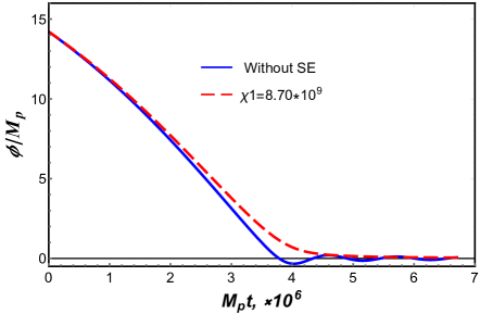
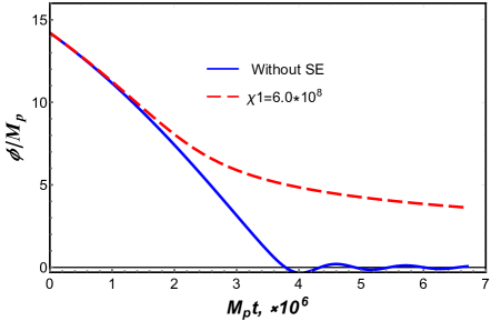
Figure 1: The time dependence of inflaton field for the simplest coupling function Eq.29 (a) and for non-minimal coupling to gravity Eq.32 (b) for different values of parameter $\chi_{1}$.Both without the Schwinger effect and with the Schwinger effect.In both figures it is obvious that strong coupling or back-reaction occurs.But in panel (b) we see that for non-minimal coupling to gravity back-reaction is much stronger.Note that in obtaining these figures we use Eq.38 for boundary term, i.e. $k_{H}=aH$.

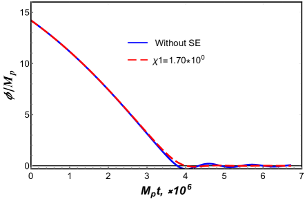
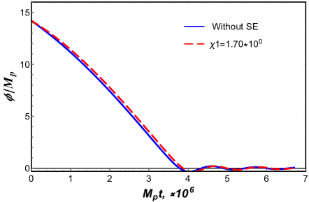
Figure 2: The time dependence of inflaton field for the simplest coupling function Eq.29 (a) and for non-minimal coupling to gravity Eq.32 (b) for the same values of parameter $\chi_{1}$.Both without the Schwinger effect and with the Schwinger effect.In panel (a) it seems that strong coupling or back-reaction does not occur.But in panel (b) we see that for non-minimal coupling to gravity back-reaction occurs and it is much stronger.Note that in obtaining these figures we use Eq.39 for boundary term $K_{H}=aH|\zeta|$ .The effect of Eq.39 is reducing the value of coupling constant $\chi_{1}$ and as we see latter in Figs of energy densities for both panels back-reaction occurs.

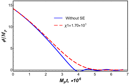
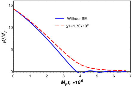
Figure 3: The time dependence of inflaton field for the simplest coupling function Eq.29 (a) and for the same coupling Eq.29 (b) for different values of parameter $\chi_{1}$.Both without(blue) the Schwinger effect and with (red)the Schwinger effect.In panel (a) it seems that strong coupling or back-reaction is weaker than panel (b).But in panel (b) we see that $\chi_{1}$ is much greater than coupling constant in panel a. Note that in obtaining panel (a) we use Eq. 39 $k_{H}=aH|\zeta|$ for boundary term , whereas in panel (b) we use Eq.38 $k_{H}=aH$.The effect of Eq. 39 $k_{H}=aH|\zeta|$ in panel (a) is reducing the value of coupling constant $\chi_{1}$.In fact, when we use tachyonic instability for $k_{H}$ the effect appears both in values of coupling constant and in strong coupling problem.We see that strong coupling problem in panel (a) is weaker than panel (b).

II.2 Mode function

Let us look at action (10).Terms $-\int d^{4}x\sqrt{-g}F_{\mu\nu}F^{\mu\nu}$ and $\int d^{4}x\sqrt{-g}F_{\mu\nu}\tilde{F}^{\mu\nu}$can be written in coulomb gauge $A_{\mu}=\left(A_{0},A_{i}\right)$ with $A_{i}=A^{T}_{i}+\partial_{i}\chi$ , where $\partial_{i}A^{T}_{i}=0$ , then the Maxwell and interaction action read

$$S_{Maxwell}+S_{Interaction}=\frac{1}{2}\int d^{4}x\left({A^{T}_{i}}^{\prime}{A^{T}_{i}}^{\prime}+A^{T}_{i}\Delta A^{T}_{i}\right)+\int d^{4}xI\left(\phi\right)\epsilon_{ijk}{A^{T}_{i}}^{\prime}\partial_{j}A^{T}_{k}$$ (23)

where $\sqrt{-g}F_{\mu\nu}\tilde{F}^{\mu\nu}=4\epsilon_{ijk}{A^{T}_{i}}^{\prime}\partial_{j}A^{T}_{k}$ and $\Delta$ is the Laplacian which is calculated respect to the Euclidean metric and $\prime$ denotes derivative with respect to the conformal time $\eta=\int\frac{dt}{a}$ .In addition , $d^{4}x=d\eta d^{3}x$.

By solving equation (23) in coulomb gauge , we achieve following relation

$${A^{T}_{i}}^{\prime\prime}-\nabla^{2}A^{T}_{i}-I^{\prime}\left(\phi\right)\epsilon_{ijk}{A^{T}_{i}}^{\prime}\partial_{j}A^{T}_{k}=0$$ (24)

The Fourier mode of equation (24) is given by following relation

$$\mathcal{A}^{\prime\prime}_{\eta}+\left(k^{2}+hkI^{\prime}\left(\phi\right)\right)\mathcal{A}_{\eta}=0$$ (25)

In terms of cosmic time , the above mode-function is given by following equation

$$\ddot{\mathcal{A}_{h}}\left(t,k\right)+H\dot{\mathcal{A}_{h}}\left(t,k\right)+\left(\frac{k^{2}}{a^{2}\left(t\right)}+h\dot{I}\left(\phi\right)\frac{{k}}{a}\right)\mathcal{A}_{h}\left(t,k\right)=0$$ (26)

In above equation $h=\pm$ shows the helicity.Also , the Fourier modes of the transverse part of vector potential can be written as $A^{T}_{i}\left(\eta,\textbf{k}\right)=\mathcal{A}_{+}\varepsilon_{+}+\mathcal{A}_{-}\varepsilon_{-}$.For more details about decomposition function in Fourier space and orthogonality relations, see our previous works in Refs.Kamarpour:2021 ; Kamarpour:2022 ; Kamarpour:2023-I .

III The Schwinger effect

We only consider expressions in strong field regime.As discussed in Refs.Kamarpour:2022 ; Kamarpour:2023 ; Kamarpour:2023-I ; Sobol-Gorbar:2021 the Schwinger effect in weak field regime is quite negligible.Thus we consider only two expressions for numerical calculations.

$$\sigma_{s}=\frac{g_{s}}{12\pi^{3}}\frac{e^{3}E}{H}\exp\left({-\frac{\pi m^{2}}{|eE|}}\right),\hskip 28.45274pts=b,f$$ (27)

In Eq.(27) , $g_{b}=1$ and $g_{f}$ are the number of spin degrees of freedom(d.o.f.).

The equation which describes created charged particles from vacuum is:

$$\dot{\rho}_{\chi}+4H\rho_{\chi}=2\rho_{E}\sigma_{s}$$ (28)

In Eq.(28) $4H$ appears because we neglect mass and only consider massless charged particles.In fact, produced charged particles due to the Schwinger effect have masses smaller than the Hubble parameter.

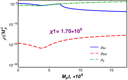
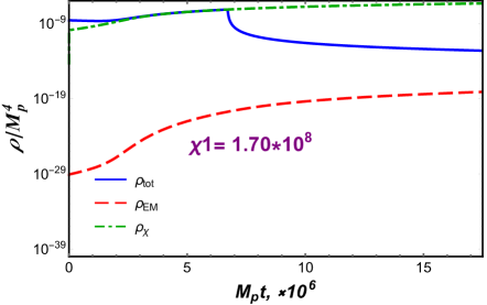
Figure 4: The time dependence (a) of energy densities for $\chi_{1}=1.70\times 10^{9}$ and the simplest coupling function Eq.29 and (b) for non-minimal coupling to gravity Eq.32 and $\chi_{1}=1.70\times 10^{8}$ .In both panels we see strong coupling or back-reaction problem due to produced charged particles. In each panel $\rho_{tot}$ (blue), $\rho_{EM}$ (red dashed line), $\rho_{\chi}$ (green dashed line ) show the total energy density, electromagnetic energy density and energy density of charged particles due to the Schwinger effect respectively.Note that electromagnetic energy density is small but the density of charged particles is very high which causes back-reaction problem.We use boundary term of Eq.38 i.e. $k_{H}=aH$ .

Figure 5: The time dependence (a) of energy densities for $\chi_{1}=1.70\times 10^{9}$ and the simplest coupling function Eq.29 and (b) for the same simplest coupling function Eq.29 and $\chi_{1}=1.70\times 10^{0}$ .In both panels we see strong coupling or back-reaction problem due to produced charged particles. In each panel $\rho_{tot}$ (blue) , $\rho_{EM}$ (red dashed line) , $\rho_{\chi}$ (green dashed line ) show the total energy density, electromagnetic energy density and energy density of charged particles due to the Schwinger effect respectively.Note that electromagnetic energy density is small but the energy density of charged particles is very high which causes back-reaction problem.We use boundary term of Eq.38 $k_{H}=aH$ for panel (a) and Eq.39 $k_{H}=aH|\zeta|$ for panel (b).As we see in Figs(2-a -b) and (3-a) , when we use tachyonic instability for $k_{H}$ the value of coupling constant reduces and effect of back-reaction is weaker than the case of standard horizon scale $k=aH$ .

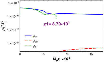
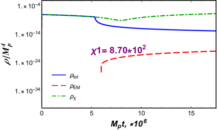
Figure 6: The time dependence (a) of energy densities for $\chi_{1}=8.70\times 10^{1}$ and non-minimal coupling function to gravity Eq.32 and (b) for the same non-minimal coupling to gravity Eq.32 and $\chi_{1}=8.70\times 10^{2}$ .In both panels we see strong coupling or back-reaction problem due to produced charged particles. In each panel $\rho_{tot}$ (blue) , $\rho_{EM}$ (red dashed line), $\rho_{\chi}$ (green dashed line ) show the total energy density, electromagnetic energy density and energy density of charged particles due to the Schwinger effect respectively.Note that electromagnetic energy density is small but the density of charged particles is very high which causes back-reaction problem.We use boundary term of Eq.39 $k_{H}=aH|\zeta|$.

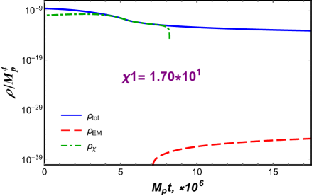
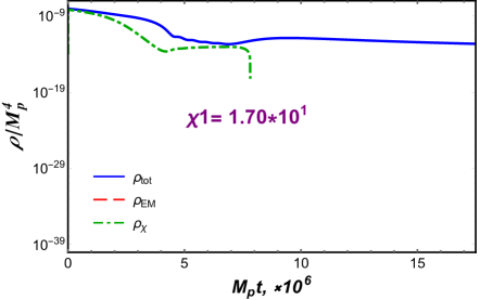
Figure 7: The time dependence (a) of energy densities for $\chi_{1}=1.70\times 10^{1}$ and the simplest coupling function Eq.29 and (b) for non-minimal coupling to gravity Eq.32 and $\chi_{1}=1.70\times 10^{1}$ .In both panels we see strong coupling or back-reaction problem due to produced charged particles. In each panel $\rho_{tot}$ (blue) , $\rho_{EM}$ (red dashed line) , $\rho_{\chi}$ (green dashed line ) show the total energy density, electromagnetic energy density and energy density of charged particles due to the Schwinger effect respectively.Note that electromagnetic energy density is small but the density of charged particles is very high which causes back-reaction problem.We use boundary term of Eq.39 $k_{H}=aH|\zeta|$.

IV Numerical calculations

IV.1 The simplest Coupling function

Before we start numerical calculations , it should be emphasized that required information about CMB constraints and slow-roll parameters such as spectral index,tensor to scalar ratio and other relevant informations $\epsilon,\eta,n_{s},r,$ are given in our previous work of RefKamarpour-Sobol:2018 . For numerical calculations it is convenient to use the following simplest coupling function.

$$I\left(\phi\right)=\chi_{1}\frac{\phi}{M_{p}}$$ (29)

In above relation $\chi_{1}$ is dimensionless coupling constant.Using this coupling function gives insight for numerical calculations.Let us look at Eq.(8).If we think of slow-roll condition then one may eliminate $\ddot{\phi}$ and $\dot{\phi}$ and obtain following relation

$$\frac{dV\left(\phi\right)}{d\phi}\sim-{I}^{\prime}\left(\phi\right)\textbf{E}\cdot\textbf{B}\sim-\frac{\chi_{1}}{M_{p}}\textbf{E}\cdot\textbf{B}$$ (30)

Using slow-roll parameter $\epsilon=\frac{M_{p}^{2}}{2}\left(\frac{V^{\prime}}{V}\right)^{2}$ and assuming in slow roll condition $\rho_{inf}\sim V\left(\phi\right)$ then we find

$$\epsilon\sim\frac{1}{2}\left(\frac{\chi_{1}\textbf{E}\cdot\textbf{B}}{\rho_{inf}}\right)^{2}$$ (31)

When we use approximation for $\textbf{E}\cdot\textbf{B}$ then the above relation will be useful.See Sobol-Gorbar:2021 .

IV.2 Non-minimal coupling to gravity

One may choose coupling function $I\left(\phi\right)$ from conformal transformation $\tilde{g}_{\mu\nu}=\Omega^{2}g_{\mu\nu}$ and achieve following relation.See Kamarpour:2021 ; Kamarpour:G ; Kamarpour:2022 ; Sobol:2021A

$$I\left(\phi\right)=12\chi_{1}e^{\left(\sqrt{\frac{2}{3}}\frac{\phi}{M_{p}}\right)}\left[\frac{1}{3M_{p}^{2}}\left(4V\left(\phi\right)\right)+\frac{\sqrt{2}}{\sqrt{3}M_{p}}\left(\frac{dV}{d\phi}\right)\right]$$ (32)

In above equation the coupling constant $\chi_{1}$ has dimension $M_{p}^{-2}$ .Inserting potential (1) into Eq.(32) the non-minimal coupling function is given by following equation

$$I\left(\phi\right)=12\chi_{1}e^{\sqrt{\frac{2}{3}}\frac{\phi}{M_{p}}}\left[\frac{4\Lambda^{4}}{3M_{p}^{2}}\left(1-\cos\left(\frac{\phi}{f}\right)\right)+\frac{\sqrt{2}}{\sqrt{3}M_{p}}\frac{\Lambda^{4}}{f}\sin\left(\frac{\phi}{f}\right)\right]$$ (33)

By taking derivative of Eq.(33) we find

$$\dot{I}\left(\phi\right)=12\dot{\phi}\chi_{1}e^{\sqrt{\frac{2}{3}}\frac{\phi}{M_{p}}}\left[\frac{\sqrt{2}}{\sqrt{3}}\frac{4\Lambda^{4}}{3M_{p}^{2}}\left(1-\cos\left(\frac{\phi}{f}\right)\right)+\frac{2}{3M_{p}^{2}}\frac{\Lambda^{4}}{f}\sin\left(\frac{\phi}{f}\right)+\frac{\sqrt{2}}{\sqrt{3}M_{p}}\frac{\Lambda^{4}}{f^{2}}\cos\left(\frac{\phi}{f}\right)\right]$$ (34)

In oder to switch on the Schwinger effect we must numerically solve equations (8 , 21 ,22 , 28 ) by using Eq.(27) into Eq.(28) and setting $\textbf{E}\cdot\textbf{B}\sim\sqrt{2\rho_{E}}\sqrt{2\rho_{B}}=2\sqrt{\rho_{E}\rho_{B}}\sim\rho_{EM}$.For this approximation we argue that in axial coupling $\rho_{E}\sim\rho_{B}$ .See Refs.Figueroa:2018 ; Notari:2016 ; Fujita:2015 ; Kamarpour:2021 ; Kamarpour:2022 ; Kamarpour:2023-I

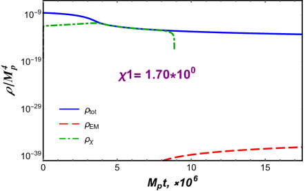
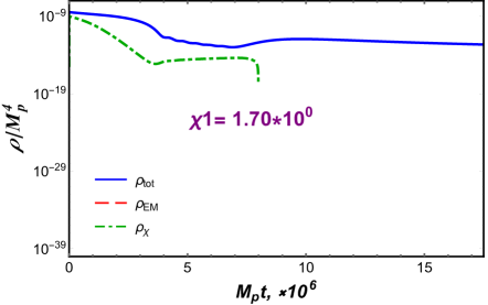
Figure 8: The time dependence (a) of energy densities for $\chi_{1}=1.70\times 10^{0}$ and the simplest coupling function Eq.29 and (b) for non-minimal coupling to gravity Eq.32 and $\chi_{1}=1.70\times 10^{0}$ .In panel (a) we see strong coupling or back-reaction problem due to produced charged particles whereas in panel (b) it seems there is no back-reaction problem.Note that in panel (b) there is no electromagnetic field at all.Therefore, for both panels the Schwinger effect is quite impossible because it spoils inflation and terminates the enhancement of electromagnetic field. In each panel $\rho_{tot}$ (blue) , $\rho_{EM}$ (red dashed line) , $\rho_{\chi}$ (green dashed line ) show the total energy density, electromagnetic energy density and energy density of charged particles due to the Schwinger effect respectively.Note that electromagnetic energy density is small but the density of charged particles is very high which causes back-reaction problem.We use boundary term of Eq.39 $k_{H}=aH|\zeta|$

.

IV.3 Tachyonic instability

We should add boundary term to the right hand side of equation (22) but we need to discuss about tachyonic instability.Le us look at Eq.(26).

Term in bracket determines tachyonic instability.Tachyonic instability begins when $h=-$ and $\dot{I}\left(\phi\right)\frac{k}{a}\geq\frac{k^{2}}{a^{2}}$ or $\frac{k}{aH}\leq\frac{{I}^{\prime}\left(\phi\right)\dot{\phi}}{H}$.We introduce the parameter $\zeta$ so that

$$\zeta=\frac{{I}^{\prime}\left(\phi\right)\dot{\phi}}{H}$$ (35)

Therefore, the condition for tachyonic instability is $\frac{k}{aH}\leq|\zeta|$.The critical value for momentum is $k_{c}=aH|\zeta|$.Thus allowed modes must satisfy $k<k_{c}$ in order to be detectable.

The above discussion will help us to add required boundary term to the right hand side of Eq.(22).

IV.4 Initial condition and boundary term

We use the Bunch-Davies vacuum initial condition for equations (25) and (26).

$$\mathcal{A}_{h}\left(t,k\right)=\frac{1}{\sqrt{2k}}e^{-ik\eta},\hskip 28.45274ptk\eta\longrightarrow\infty$$ (36)

Power spectrum of electric field is defined bySubramanian:2016 ; Durrer:2013

$$\frac{d\rho_{E}}{d\ln k}=\frac{k^{3}}{\left(2\pi\right)^{2}}\frac{1}{a^{2}}\left(|\frac{\partial\mathcal{A}_{+}(t,k)}{\partial t}|^{2}+|\frac{\partial\mathcal{A}_{-}(t,k)}{\partial t}|^{2}\right).$$ (37)

Using Eq.(37) we find required equation for boundary termSobol:2018 ; Kamarpour:2022 ; Kamarpour:2023 ; Kamarpour:2023-I .

$$\left(\dot{\rho}_{E}\right)_{H}=\frac{d\rho_{E}}{dk}\arrowvert_{k=k_{H}}\cdot\frac{dk_{H}}{dt}=\frac{H^{5}}{8\pi^{2}},\hskip 14.22636ptk_{H}=aH$$ (38)

One writes Eq.(38)by setting $k_{H}=k_{c}=aH|\zeta|$ .Thus the required relation for boundary term is given bySobol-Gorbar:2021 .

$$\left(\dot{\rho}_{E}\right)_{H}=\frac{d\rho_{E}}{dk}\arrowvert_{k=k_{H}}\cdot\frac{dk_{H}}{dt}=\frac{H^{5}|\zeta|^{3}}{\pi^{2}},\hskip 14.22636ptk_{H}=k_{c}=aH|\zeta|$$ (39)

We must emphasize that the Eqs.(38) or (39) should be added to the right hand side of Eq.(22) separately in order to investigate which one is more appropriate choice.

All remains to be done is to solve Eqs.(21 , 8 , 22 , 28) and to obtain required results.Before that let us look at figures.

Figure (1 , 2 , 3) show the time dependence of inflation field without Schwinger effect (blue line )and with Schwinger effect (red dashed line) for various values of parameter $\chi_{1}$. Note that for $\chi_{1}=1.70\times 10^{0}$ it seems the back-reaction is weak and there is possibility for the Schwinger effect whereas in figure 8 we see the energy density of produced charged particle is high and the Schwinger effect does not occur.In addition in figure 8 electromagnetic field is very small .

Figure (4) shows the time dependence (a) of energy densities for $\chi_{1}=1.70\times 10^{9}$ and (b) for $\chi_{1}=1.70\times 10^{8}$.There is back-reaction in each panels. In each panel $\rho_{tot}$ (blue), $\rho_{{}_{E}}$ (red dashed line), $\rho_{\chi}$ (green dashed line ) show the total energy density, electromagnetic energy density and energy density of charged particles due to Schwinger effect respectively.We identify the horizon scale by $k_{H}=aH$.

Figure (5) shows the time dependence (a) of energy densities for $\chi_{1}=1.70\times 10^{9}$ and (b) for $\chi_{1}=1.70\times 10^{0}$. In both panels we see back-reaction due to produced charged particles respectively. In each panel $\rho_{tot}$ (blue) ,$\rho_{{}_{E}}$ (red dashed line), $\rho_{\chi}$ (green dashed line ) show the total energy density, electromagnetic energy density and energy density of charged particles due to Schwinger effect respectively. We see that electromagnetic energy densities are very small and also energy densities of created charged particles for these value of parameter $\chi_{1}$ are high and causes back-reaction .

Figure (6) shows the time dependence(a) of energy densities for $\chi_{1}=1.70\times 10^{1}$ and (b) $\chi_{1}=8.70\times 10^{2}$.In both panel we use Eq.(32) for coupling function.In each panel $\rho_{tot}$ (blue) , $\rho_{{}_{E}}$ (red dashed line), $\rho_{\chi}$ (green dashed line ) show the total energy density, electromagnetic energy density and energy density of charged particles due to Schwinger effect respectively.Also in both panel we identify the horizon scale by $k_{H}=aH|\zeta|$.Electromagnetic energy densities in both panels are very small but energy densities of produced charged particles are exceeding of energy density of inflaton field.

Figure ( 8 ) shows when Schwinger effect is on there is no electromagnetic filed in panel (b) and in panel(a) is not significant.

More importantly,let us look at figures (2- a) and (8- b).It seems back-reaction is weak and the Schwinger effect exists.In both figures $k_{H}=aH|\zeta|$ in order to avoid back-reaction problem.But we discovered that there is no significant electromagnetic field.Thus the Schwinger effect plays no roles because of strong coupling problem and instead spoils inflaton field.

V Conclusion

In this work we examined the influence of the Schwinger effect on natural inflation model by axial coupling.Our study was divided into two parts.

In first part , we assumed $\rho_{E}\sim\rho_{B}$ and for this reason we only included $\rho_{EM}$ in the Friedmann equation (21).This assumption was validated by considering axial coupling between electromagnetic field and inflaton field.In addition, the correctness of this assumption was mentioned and confirmed in literature before Figueroa:2018 ; Notari:2016 ; Fujita:2015 ; Kamarpour:2021 ; Kamarpour:2022 ; Kamarpour:2023-I .

We used two coupling functions , the simplest coupling of Eq.(29) and non-minimal coupling to gravity Eq.(32).In first part ,we incorporated the Schwinger effect in our action and considered the equation of motion for the inflaton field , taking into account the back-reaction term $\textbf{E}\cdot\textbf{B}$ in the right hand side of equation (8) and added a gauge invariant action to the action 3.Then we finalized system of closed equations and performed numerical calculations by utilizing the coupling functions (29 , 32) and boundary term (38) in relations (21 , 8 , 22 , 28).

We produced figures (1 , 2 ,3 , 4 , 5 , 6 , 7 , 8) and observed that when the horizon scale is $k_{H}=aH$ , back-reaction occurs due to created charged particles.In fact,we found that instantly, the Schwinger effect produces very high energy density of charged particles which causes back-reaction problem.

In second part,we activated another boundary term in order to avoid back-reaction problem.Thus, we adhered to our assumption of $\rho_{B}\sim\rho_{E}$, and accordingly, only electromagnetic energy density $\rho_{EM}$ was included in the Friedmann equation (21) and identified the new horizon scale $K_{H}=aH|\zeta|,\zeta=\frac{{I}^{\prime}\left(\phi\right)\dot{\phi}}{H}$ .This is the scale at which a given Fourier mode Eq.(26) begins to become tachyonically unstable.But choosing this scale does not alter conclusions of the first part.

Subsequently, we performed numerical calculations and noticed that ,the effect of choosing tachyonic instability is reducing the values of coupling constant $\chi_{1}$ and also weakening the back-reaction problem.Therefore, in this investigation we found that the Schwinger effect does not occur because of strong coupling or back-reaction.

Finally,in contrast to our previous works in Refs.Kamarpour-Sobol:2018 ; Kamarpour:2023 on natural inflation model in which both magneto-genesis and the Schwinger effect were considerable,in this work we discovered that in axial coupling at least the Schwinger effect is impossible and spoils inflaton field.

One may estimate due to existence of strong back-reaction problem , magneto-genesis by axial coupling in this model is impossible.But this needs separate investigation and should be addressed elsewhere.

Data Availability Statement

The Author confirms that this manuscript has no associated data in a data repository.

Declaration of competing interest

The authors declare that they have no known competing financial interests or personal relationships that could have appeared to influence the work reported in this paper.

References

References

- (1) M. Kamarpour, O. Sobol. Magnetogenesis in Natural inflation model. Ukr. J. Phys. 63(8):673 (2018). https://doi.org/10.15407/ujpe63.8.673
- (2) M. Kamarpour, The Schwinger effect and Natural inflationary magnetogenesis.Gen Relativ Gravit 55, 27 (2023). https://doi.org/10.1007/s10714-023-03081-z.
- (3) P.P. Kronberg. Extragalactic magnetic fields. Rep. Prog. Phys. 57, 325 (1994).
- (4) D. Grasso and H.R. Rubinstein. Magnetic fields in the early universe. Phys. Rep. 348, 163 (2001).
- (5) L.M. Widrow. Origin of galactic and extragalactic magnetic fields. Rev. Mod. Phys. 74, 775 (2002).
- (6) M. Giovannini. The magnetized universe. Int. J. Mod. Phys. D 13, 391 (2004).
- (7) A. Kandus, K.E. Kunze, and C. G. Tsagas. Primordial magnetogenesis. Phys. Rep. 505, 1 (2011).
- (8) R. Durrer and A. Neronov. Cosmological magnetic fields: their generation, evolution and observation. Astron. Astrophys. Rev. 21, 62 (2013).
- (9) K. Subramanian. The origin, evolution and signatures of primordial magnetic fields. Rep. Prog. Phys. 79, 076901 (2016).
- (10) N. Aghanim et al. (Planck Collaboration): Planck 2018 results. VI. Cosmological parameters, arXiv:1807.06209v1.
- (11) P.A.R. Ade et al. (Planck Collaboration). Planck 2015 results. XX. Constraints on inflation. Astron. Astrophys. 594, A20 (2016).
- (12) D.R. Sutton, C. Feng, and C.L. Reichardt. Current and future constraints on primordial magnetic fields. Astrophys. J. 846, 164 (2017).
- (13) K. Jedamzik and A. Saveliev. A stringent limit on primordial magnetic fields from the cosmic microwave backround radiation. arXiv:1804.06115 [astro-ph.CO].
- (14) A. Neronov and I. Vovk. Evidence for strong extragalactic magnetic fields from Fermi observations of TeV blazars. Science 328, 73 (2010).
- (15) F. Tavecchio, G. Ghisellini, L. Foschini et al. The intergalactic magnetic field constrained by Fermi/LAT observations of the TeV blazar 1ES 0229+200. Mon. Not. R. Astron. Soc. 406, L70 (2010).
- (16) A.M. Taylor, I. Vovk, and A. Neronov. Extragalactic magnetic fields constraints from simultaneous GeV-TeV observations of blazars. Astron. Astrophys. 529, A144 (2011).
- (17) C. Caprini and S. Gabici. Gamma-ray observations of blazars and the intergalactic magnetic field spectrum. Phys. Rev. D 91, 123514 (2015).
- (18) L. Biermann. Über den Ursprung der Magnetfelder auf Sternen und im interstellaren Raum. (About the origin of the magnetic fields on stars and in the interstellar space). Z. Naturforsch. A5, 65 (1950).
- (19) Ya.B. Zeldovich, A.A. Ruzmaikin, and D.D. Sokoloff. Magnetic Fields in Astrophysics (Gordon and Breach, New York, 1990).
- (20) H. Lesch, M. Chiba. Protogalactic evolution and magnetic fields. Astron. Astrophys. 297, 305 (1995).
- (21) R. Kulsrud, S.C. Cowley, A.V. Gruzinov et al. Dynamos and cosmic magnetic fields. Phys. Rep. 283, 213 (1997).
- (22) S.A. Colgate and H. Li. The origin of the magnetic fields of the universe: The plasma astrophysics of the free energy of the universe. Phys. Plasmas 8, 2425 (2001) .
- (23) M.J. Rees. The origin and cosmogonic implications of seed magnetic fields. Quaterly J. R. Astr. Soc. 28, 197 (1987).
- (24) R.A. Daly and A. Loeb. A possible origin of galactic magnetic fields. Astrophys. J. 364, 451 (1990).
- (25) T.A. Ensslin, P.L. Biermann, P.P. Kronberg et al. Cosmic-ray protons and magnetic fields in clusters of galaxies and their cosmological consequences. Astrophys. J. 477, 560 (1997).
- (26) S. Bertone, C. Vogt, and T. Ensslin. Magnetic field seeding by galactic winds. Mon. Not. R. Astron. Soc. 370, 319 (2006).
- (27) M.S. Turner and L.M. Widrow. Inflation-produced, large-scale magnetic fields. Phys. Rev. D 37, 2743 (1988).
- (28) B. Ratra. Cosmological seed magnetic field from inflation. Astrophys. J. 391, L1 (1992).
- (29) C.J. Hogan. Magnetohydrodynamic effects of a first-order cosmological phase transition. Phys. Rev. Lett. 51, 1488 (1983).
- (30) J.M. Quashnock, A. Loeb, and D.N. Spergel. Magnetic field generation during the cosmological QCD phase transition. Astrophys. J. 344, L49 (1989).
- (31) T. Vachaspati. Magnetic fields from cosmological phase transitions. Phys. Lett. B 265, 258 (1991).
- (32) V.F. Mukhanov and G.V. Chibisov. Quantum fluctuations and a nonsingular universe. JETP Lett. 33, 532 (1981).
- (33) S.W. Hawking. The development of irregularities in a single bubble inflationary universe. Phys. Lett. B 115, 295 (1982).
- (34) A.A. Starobinsky. Dynamics of phase transition in the new inflationary universe scenario and generation of perturbations. Phys. Lett. B 117, 175 (1982).
- (35) A.H. Guth and S.Y. Pi. Fluctuations in the new inflationary Universe. Phys. Rev. Lett. 49, 1110 (1982).
- (36) J.M. Bardeen, P.J. Steinhardt, and M.S. Turner. Spontaneous creation of almost scale-free density perturbations in an inflationary universe. Phys. Rev. D 28, 679 (1983).
- (37) L.P. Grishchuk. Amplification of gravitational waves in an isotropic universe. Sov. Phys. JETP 40, 409 (1975).
- (38) A.A. Starobinsky. Spectrum of relict gravitational radiation and the early state of the Universe. JETP Lett. 30, 682 (1979).
- (39) V.A. Rubakov, M.V. Sazhin, and A.V. Veryaskin. Graviton creation in the inflationary Universe and the grand unification scale. Phys. Lett. B 115, 189 (1982).
- (40) L. Parker. Particle creation in expanding universes. Phys. Rev. Lett. 21, 562 (1968).
- (41) A.D. Dolgov. Breaking of conformal invariance and electromagnetic field generation in the universe. Phys. Rev. D 48, 2499 (1993).
- (42) M. Gasperini, M. Giovannini, and G. Veneziano. Primordial magnetic fields from string cosmology. Phys. Rev. Lett. 75, 3796 (1995).
- (43) M. Giovannini. Magnetogenesis and the dynamics of internal dimensions. Phys. Rev. D 62, 123505 (2000).
- (44) K. Atmjeet, I. Pahwa, T.R. Seshadri et al. Cosmological magnetogenesis from extra-dimensional Gauss-Bonnet gravity. Phys. Rev. D 89, 063002 (2014).
- (45) T. Fujita, R. Namba, Y. Tada, N. Takeda, and H. Tashiro, Consistent generation of magnetic fields in axion inflation models, J. Cosmol. Astropart. Phys. 05 (2015) 054 [arXiv: 1503.05802 [astro-ph.CO]].
- (46) A. Notari and K. Tywoniuk, Dissipative axial inflation, J. Cosmol. Astropart. Phys. 12 (2016) 038 [arXiv: 1608.06223 [hep-th]].
- (47) J.R. Canivete Cuissa and D.G. Figueroa, Lattice formulation of axion inflation. Application to preheating, J. Cosmol. Astropart. Phys. 06 (2019) 002 [arXiv: 1812.03132 [astro-ph.CO]].
-
(48)
M. Kamarpour: Magnetogenesis in Higgs inflation model, Gen. Relativ. Gravit. 53, https:
doi.org/10.1007/s10714-021-02824-0 (2021). - (49) M. Kamarpour: Influence of the Schwinger effect on radiatively corrected Higgs inflationary magnetogenesis, Gen Relativ Gravit 54, 32 (2022). https://doi.org/10.1007/s10714-022-02920-9.
- (50) M. Kamarpour: The alteration of the Schwinger effect on radiatively corrected Higgs inflationary magneto-genesis by axial coupling,IJMPD-Vol.32, No 05,2350025.(2023).https://doi.org/10.1142/S0218271823500256
- (51) M. Giovannini. On the variation of the gauge couplings during inflation. Phys. Rev. D 64, 061301 (2001).
- (52) K. Bamba and J. Yokoyama. Large scale magnetic fields from inflation in dilaton electromagnetism. Phys. Rev. D 69, 043507 (2004).
- (53) J. Martin and J. Yokoyama. Generation of large-scale magnetic fields in single-field inflation. J. Cosmol. Astropart. Phys. 01, 025 (2008).
- (54) V. Demozzi, V.M. Mukhanov, and H. Rubinstein. Magnetic fields from inflation? J. Cosmol. Astropart. Phys. 08, 025 (2009).
- (55) S. Kanno, J. Soda, and M. Watanabe. Cosmological magnetic fields from inflation and backreaction. J. Cosmol. Astropart. Phys. 12, 009 (2009).
- (56) R.J.Z. Ferreira, R.K. Jain, and M.S. Sloth. Inflationary magnetogenesis without the strong coupling problem. J. Cosmol. Astropart. Phys. 10, 004 (2013).
- (57) R.J.Z. Ferreira, R.K. Jain, and M.S. Sloth. Inflationary magnetogenesis without the strong coupling problem II: Constraints from CMB anisotropies and B-modes. J. Cosmol. Astropart. Phys. 06, 053 (2014).
- (58) S. Vilchinskii, O. Sobol, E.V. Gorbar et al. Magnetogenesis during inflation and preheating in the Starobinsky model. Phys. Rev. D 95, 083509 (2017).
- (59) O.O Sobol,E.V. Gorbar,S.I. Vilchinskii:Backreaction of electromagnetic fields and the Schwinger effect in pseudoscalar inflation magnetogenesis,Phys. Rev. D 100, 063523.(2019).arXiv:1907.10443v2 [astro-ph.CO].
- (60) J. Schwinger: On gauge invariance and vacuum polarization, https://doi.org/10.1103/PhysRev.82.664 Phys. Rev. 82, 664 (1951).
- (61) T. Kobayashi and N. Afshordi: Schwinger effect in 4D de Sitter space and constraints on magnetogenesis in the early Universe. J. High Energy Phys. 10,166(2014)
- (62) C. Stahl: Schwinger effect impacting primordial magnetogenesis, Nucl.Phys.B939,95,(2018), arXiv: 1806.06692[hep-th].
- (63) J.-J. Geng, B.-F. Li, J. Soda, A. Wang, Q. Wu, and T. Zhu: Schwinger pair production by electric field coupled to inflaton, https://doi.org/10.1088/1475-7516/2018/02/018 J. Cosmol. Astropart. Phys. 02 (2018) 018 [arXiv: 1706.02833 [gr-qc]].
- (64) M.B. Fröb, J. Garriga, S. Kanno, M. Sasaki, J. Soda, T. Tanaka, and A. Vilenkin: Schwinger effect in de Sitter space, https://doi.org/10.1088/1475-7516/2014/04/009 J. Cosmol. Astropart. Phys. 04 (2014) 009 [arXiv: 1401.4137 [hep-th]].
- (65) E. Bavarsad, C. Stahl, and S.-S. Xue: Scalar current of created pairs by Schwinger mechanism in de Sitter spacetime. Phys. Rev. D 94, 104011 (2016).
- (66) C. Stahl, E. Strobel, and S.-S. Xue: Fermionic current and Schwinger effect in de Sitter spacetime, https://doi.org/10.1103/PhysRevD.93.025004 Phys. Rev. D 93, 025004 (2016)
- (67) C. Stahl and S.-S. Xue: Schwinger effect and backreaction in de Sitter spacetime, https://doi.org/10.1016/j.physletb.2016.07.011 Phys. Lett. B 760, 288 (2016)
- (68) T. Hayashinaka, T. Fujita, and J. Yokoyama: Fermionic Schwinger effect and induced current in de Sitter space, https://doi.org/10.1088/1475-7516/2016/07/010 J. Cosmol. Astropart. Phys. 07 (2016) 010 [arXiv: 1603.04165 [hep-th]].
- (69) T. Hayashinaka and J. Yokoyama: Point splitting renormalization of Schwinger induced current in de Sitter spacetime, https://doi.org/10.1088/1475-7516/2016/07/012 J. Cosmol. Astropart. Phys. 07 (2016) 012 [arXiv: 1603.06172 [hep-th]].
- (70) R. Sharma and S. Singh: Multifaceted Schwinger effect in de Sitter space, https://doi.org/10.1103/PhysRevD.96.025012 Phys. Rev. D 96, 025012 (2017) [arXiv: 1704.05076 [gr-qc]].
- (71) W. Tangarife, K. Tobioka, L. Ubaldi, and T. Volansky: Dynamics of relaxed inflation, https://doi.org/10.1007/JHEP02(2018)084 J. High Energy Phys. 02 (2018) 084 [arXiv: 1706.03072 [hep-ph]].
- (72) E. Bavarsad, S.P. Kim, C. Stahl, and S.-S. Xue: Effect of a magnetic field on Schwinger mechanism in de Sitter spacetime, https://doi.org/10.1103/PhysRevD.97.025017 Phys. Rev. D 97, 025017 (2018) [arXiv: 1707.03975 [hep-th]].
- (73) T. Hayashinaka and S.-S. Xue: Physical renormalization condition for de Sitter QED, https://doi.org/10.1103/PhysRevD.97.105010 Phys. Rev. D 97, 105010 (2018) [arXiv: 1802.03686 [gr-qc]].
- (74) T. Hayashinaka: Analytical Investigation into electromagnetic Response of Quantum Fields in de Sitter Spacetime, Ph.D. thesis, University of Tokyo, 2018.
- (75) M. Giovannini: Spectator electric fields, de Sitter spacetime, and the Schwinger effect, https://doi.org/10.1103/PhysRevD.97.061301 Phys. Rev. D 97, 061301(R) (2018) [arXiv: 1801.09995 [hep-th]].
- (76) H. Kitamoto: Schwinger effect in inflaton-driven electric field, https://doi.org/10.1103/PhysRevD.98.103512 Phys. Rev. D 98, 103512 (2018) [arXiv: 1807.03753 [hep-th]].
- (77) K. Freese, J.A. Frieman, and A.V. Olinto. Natural inflation with pseudo Nambu-Goldstone bosons. Phys. Rev. Lett. 65, 3233 (1990).
- (78) F.C. Adams, J.R. Bond, K. Freese et al. Natural inflation: Particle physics models, power-law spectra for large-scale structure, and constraints from the Cosmic Background Explorer. Phys. Rev. D 47, 426 (1993).
- (79) O.O. Sobol, E.V. Gorbar, M. Kamarpour, and S.I. Vilchinskii: Influence of backreaction of electric fields and Schwinger effect on inflationary magnetogenesis, https://doi.org/10.1103/PhysRevD.98.063534 Phys. Rev. D 98, 063534 (2018) [arXiv: 1807.09851 [hep-ph]].
- (80) M. Kamarpour: Magnetogenessis by non-minimal coupling to gravity in Higgs inflation model, Ann. Phys. 428,168459,2021.
- (81) O.O. Sobol, E.V. Gorbar, O.M. Teslyk, S.I. Vilchinskii: Generation of electromagnetic field nonminimally coupled to gravity during the Higgs inflation. Phys. Rev. D 104, 043509 (2021). [arXiv:2014.14400v1[gr-qc]].