Analysis of Task Transferability in Large Pre-trained Classifiers

Abstract

Transfer learning transfers the knowledge acquired by a model from a source task to multiple downstream target tasks with minimal fine-tuning. The success of transfer learning at improving performance, especially with the use of large pre-trained models has made transfer learning an essential tool in the machine learning toolbox. However, the conditions under which the performance is transferable to downstream tasks are not understood very well. In this work, we analyze the transfer of performance for classification tasks, when only the last linear layer of the source model is fine-tuned on the target task. We propose a novel Task Transfer Analysis approach that transforms the source distribution (and classifier) by changing the class prior distribution, label, and feature spaces to produce a new source distribution (and classifier) and allows us to relate the loss of the downstream task (i.e., transferability) to that of the source task. Concretely, our bound explains transferability in terms of the Wasserstein distance between the transformed source and downstream task’s distribution, conditional entropy between the label distributions of the two tasks, and weighted loss of the source classifier on the source task. Moreover, we propose an optimization problem for learning the transforms of the source task to minimize the upper bound on transferability. We perform a large-scale empirical study by using state-of-the-art pre-trained models and demonstrate the effectiveness of our bound and optimization at predicting transferability. The results of our experiments demonstrate how factors such as task relatedness, pretraining method, and model architecture affect transferability.

1 Introduction

Transfer learning [32, 46] has emerged as a powerful tool for developing high-performance machine learning models in scenarios when sufficient labeled data is unavailable or when training large models is computationally challenging. Since large pre-trained models are becoming the cornerstone of machine learning [35, 8, 9, 7, 16, 19], understanding when the knowledge gathered by these models improves the performance of a downstream task is becoming crucial. While the large pre-trained models achieve high performance even in the zero-shot inference settings [35], their performance can be further improved by fine-tuning them on the downstream tasks. However, due to the size of these models, fine-tuning all the layers of the models is computationally challenging and expensive. On the other hand, fine-tuning/learning only a linear layer on top of the representations from these models is both efficient and effective and is the focus of our work.

While transfer learning achieves remarkable success the reasons for its success are not clearly understood. Previous analytical [5, 4, 41, 28, 25, 29, 30] works such as those based on domain adaptation have studied the problem of covariate/label shifts between the tasks. But they are not applicable to transfer learning since the crucial assumption of the same feature and label sets between the source and target tasks is not necessary for transfer learning. Another recent line of work [44, 48, 43, 22] estimates the transfer learning performance (transferability) of the models by proposing metrics that can be computed more efficiently than fine-tuning. But insights obtained from these metrics into how transferability relates to the source data used for training the encoder are rather limited.

To relate the source and the target tasks, our analysis first transforms the source distribution (along with the classifier of the source task) by transforming its class-prior distribution, label set, and feature space (Fig. 1) to obtain the transformed distribution. Under this simple model, we first show that the performance on the transformed source is directly related to the performance of the original source task (Theorem 1). However, real distributions of the target downstream tasks may not be transforms of the source task, and hence the transformed source distribution could still have a mismatch with the distribution of the target task. We explain the residual mismatch between the transformed source and target through the distributional divergence metrics such as the Wasserstein distance [34, 45]. This leads to our Theorem 2, which relates transferability to the performance of the transformed source distribution and type-1 Wasserstein distance between the two joint distributions. Finally, the results from the two previous theorems allow us to explain the transferability to a target task as a sum of three intuitive terms (Theorem 3), namely, the reweighted source loss (due to a class prior distribution differences between tasks), a label mismatch term (as conditional entropy between the label distributions of the tasks) and a distribution mismatch term (as Wasserstein distance).

The proposed upper bound can be minimized by learning the parameters of the transforms by using samples from the source and target tasks. Thus, we propose an optimization problem that learns transform parameters by minimizing the residual Wasserstein distance between the transformed source and the target distribution. To demonstrate the effectiveness of our analytical results in predicting transferability and the effectiveness of our optimization problem in learning transforms to minimize the upper bound we present a large-scale empirical study (Sec. 4) with large pre-trained models trained with different architectures (ResNet [21], ViT [17]), pretraining methods (CLIP [35], MAE [19], SimCLR [8], DistilBERT [39]), and datasets (Imagenet [15], CIFAR10/100 [23], Aircraft [27], Pets [33] and DTD [10]).

The results of our experiments show that our upper bound effectively predicts transferability for any transform in the set of valid transforms (Sec. 3). Moreover, learning the transforms by solving the proposed optimization problem produces a significantly better upper bound. Our results also highlight the effect of the relatedness of the source and target downstream tasks (measured in terms of the distribution mismatch and label space mismatch) on the transferability. Specifically, related tasks can be transformed in a way that the residual mismatch between the transformed source and target distribution can be reduced thereby leading to a smaller gap between the empirical and predicted transferability. Thus, our analytical results suggest that the source task used for training the large pretrained models can be used to explain transferability downstream tasks. The insights from this analysis can be used to further improve the transferability of the models.

Our main contributions are summarized as follows:

• We propose a task transfer analysis approach for analyzing the success of transfer learning with linear fine-tuning for classification tasks. Using this approach we find that transferability can be explained in terms of the reweighted source loss, a label mismatch term, and a distribution mismatch term.

• We propose and solve a novel optimization problem that learns the parameters of the transform to transfer the source task to the target task. Transforms learned through our optimization effectively minimize the proposed upper bound on transferability.

• We provide a large-scale empirical analysis of transferability with state-of-the-art large pre-trained models on standard transfer learning tasks. Through this, we study how various transforms, relatedness between the source and target tasks, pretraining method, and model architecture affect the different terms of our proposed upper bound.

2 Related Work

Transfer learning: Transfer learning has been shown to achieve promising results across many areas of machine learning [32, 46] including natural language processing (NLP) [16, 39] and computer vision [36, 13]. Recent works have demonstrated that the transferability of models improves when trained with pretraining methods such as adversarial training [38], self-supervised learning [8, 7, 9] and by combining language and image information [35]. The success of these is explained in terms of different training methods helping learn an improved feature representation.

Analytical results for learning under distribution shifts: Prior works [5, 4, 41, 28, 25, 29, 30] explained the success of learning in the presence of distribution shifts in terms of the distributional divergence between the marginal distributions and a label mismatch term. However, these results are applicable under assumptions such as covariate shift or label shift which need not be satisfied by transfer learning where both the data distribution and the label spaces can be different. Other works [6, 37] exploited task-relatedness at improving multi-task learning. These prior works showed that when tasks are weakly related, learning a single model does not perform well for both tasks. Our analytical results illustrate the same effect of task-relatedness on transferability.

Transferability estimation: This line of work [44, 3, 31, 22, 48, 43] assumes access to labeled data from the target task and estimates the transferability of pre-trained models without fine-tuning. [44] proposed the Negative Conditional Entropy (NCE) score that estimates transferability through the negative conditional entropy between labels of the tasks but requires the tasks to have the same input instances. [31] proposed LEEP score and computed NCE using soft labels for the target task from a pre-trained model. OT-CE [43] combined Wasserstein distance [1] and NCE score whereas [3, 48] estimate likelihood and the marginalized likelihood of labeled target examples to estimate transferability. However, these metrics can only be used for post hoc analysis and do not provide many insights into how transferability is related to the source task used for training the classifier or how the source model should be trained to achieve better transferability. Different from most of these works, our goal is not to only measure transferability but to rigorously relate transferability to downstream tasks in a general transfer learning setting back to the source task.

3 Analysis of task transferability

Problem setting and notations: Let $P_{S}(x,y)$ and $P_{T}(x,y)$ denote the distributions of the source task and the target task, defined on $\mathcal{X}_{S}\times\mathcal{Y}_{S}$ and $\mathcal{X}_{T}\times\mathcal{Y}_{T}$ respectively. We assume that the feature spaces are common ($\mathcal{X}_{S}=\mathcal{X}_{T}=\mathcal{X}$) such as RGB images, but the source label set $\mathcal{Y}_{S}=\{1,2,\cdots,K_{S}\}$ and the target label set $\mathcal{Y}_{T}=\{1,2,\cdots,K_{T}\}$ can be entirely different to allow for arbitrary (unknown) downstream tasks. We assume the number of source classes ($K_{S}$) is greater than or equal to the number of target classes ($K_{T}$). In the transfer learning setting, an encoder $g:\mathcal{X}\rightarrow\mathcal{Z}$ is first (pre)trained with source data with or without the source labels depending on the training method (e.g., supervised vs self-supervised). We denote the resultant push-forward distributions of $S$ and $T$ on the encoder output space as $P_{S}(z,y)$ and $P_{T}(z,y)$. With this fixed representation, a linear softmax classifier $h(z):\mathcal{Z}\rightarrow\Delta$ that outputs a probability vector is learned for the source ($h_{S}(z)$) and for the downstream target ($h_{T}(z)$) separately, where $\Delta_{S/T}$ is a $K_{S}/K_{T}$ simplex for $S/T$, respectively. The linear fine-tuning is done by $\min_{h_{S}}\mathbb{E}_{(z,y)\in P_{S}}[\ell(h_{S}(z),y)]$ and $\min_{h_{T}}\mathbb{E}_{(z,y)\in P_{T}}[\ell(h_{T}(z),y)]$ with empirical distributions using the cross entropy loss: $\ell(h(z),y)=-w_{y}^{T}z+\log\sum_{i}e^{w_{i}^{T}z}$. We present all the proofs for this section in App. A.

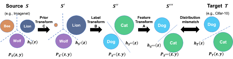
Figure 1: A series of transforms are applied to the source distribution $P_{S}(z,y)$ and classifier $h_{S}$ to produce the transformed distribution $P_{S^{\prime\prime\prime}}$ and classifier $h_{S^{\prime\prime\prime}}$ making it comparable to those of a downstream target task. Prior transform ($S\rightarrow S^{\prime}$) changes the class prior of the source distribution (e.g, an irrelevant Bee class in $S$ now has smaller prior) followed by label set transform ($S^{\prime}\rightarrow S^{\prime\prime}$) (e.g., to match $\{$Lion, Wolf$\}$ with $\{$Cat, Dog$\}$), followed by feature space transform ($S^{\prime\prime}\rightarrow S^{\prime\prime\prime}$) to match the feature distribution $P_{T}(z,y)$. These simple transformations allow us to effectively analyze task transferability after linear finetuning.

3.1 The task transfer analysis model for analyzing transferability

The source and the target tasks share the same encoder but do not share label sets or the data distributions. Therefore, to relate the two tasks, we propose a chain of three simple transforms: 1) prior transform (from $S$ to $S^{\prime}$), 2) label transform (from $S^{\prime}$ to $S^{\prime\prime}$), and 3) feature transform (from $S^{\prime\prime}$ to $S^{\prime\prime\prime}$). The $S^{\prime},S^{\prime\prime},S^{\prime\prime\prime}$ are intermediate domain names after each of the transforms are applied. The corresponding classifier $h$ in each domain is also denoted by $h_{S^{\prime}}$, $h_{S^{\prime\prime}}$, and $h_{S^{\prime\prime\prime}}$. This chain is illustrated in Fig. 1. The distribution after the transform $P_{S^{\prime\prime\prime}}$ has the same feature $\mathcal{Z}_{S^{\prime\prime\prime}}=\mathcal{Z}_{T}=\mathcal{Z}$ and label sets $\mathcal{Y}_{S^{\prime\prime\prime}}=\mathcal{Y}_{T}$ as the target task $T$, and consequently, the loss of the transformed classifier $h_{S^{\prime\prime\prime}}$ can be directly related to the loss of the target classifier $h_{T}$.

3.1.1 Prior transform $(S\rightarrow S^{\prime})$

In transfer learning, it is common that the source task has more classes than the target task ($|\mathcal{Y}_{S}|\geq|\mathcal{Y}_{T}|$). Furthermore, it is highly likely that many of the source classes are not relevant to or useful for the target classes. For example, to transfer from Imagenet to CIFAR10, only a small portion of the source classes are relevant to the target classes. The prior transform accounts for the importance of the source classes. This is illustrated in Fig. 1 where changing the class prior of $S$ reduces the prior of the Bee class to near zero and increases the priors of classes Wolf and Lion (shown by the changed size of classes Wolf and Lion). While we transform the prior of $S$, we keep the conditional distribution to be the same ($P_{S^{\prime}}(z|y)=P_{S}(z|y)$) and also keep the classifier the same ($h_{S^{\prime}}(z)=h_{S}(z)$). The Lemma 1 describes how the expected loss of the classifier $h_{S}$ between the domains $S$ and $S^{\prime}$ are related after applying the prior transform.

Lemma 1.

Let $C:=\left[\frac{P_{S^{\prime}}(y)}{P_{S}(y)}\right]_{y=1}^{|\mathcal{Y}_{S}|}$ be a vector of probability ratios and the classifier $h_{S^{\prime}}(z):=h_{S}(z)$, then we have $\mathbb{E}_{P_{S^{\prime}}(z,y)}[\ell(h_{S^{\prime}}(z),y)]=\mathbb{E}_{P_{S}(z,y)}[C(y)\ell(h_{S}(z),y)],\;$ for any loss function $\ell$.

Lemma 1 shows that the expected loss in the new domain $S^{\prime}$ is simply a reweighted version of the loss on the source domain $S$ with the classifier $h_{S}$.

3.1.2 Label transform $(S^{\prime}\rightarrow S^{\prime\prime})$

Next, we apply a label transform so that the label set of the new domain $S^{\prime\prime}$ match the label set of the downstream target domain. To change the label set of the domain $S^{\prime}$, we specify the conditional distribution $B_{ij}:=P(y_{S^{\prime\prime}}=i|y_{S^{\prime}}=j)$ ($0\leq B_{ij}\leq 1,\;\forall\;i,j,\;\;\sum_{i}B_{ij}=1,\;\forall i$). Note that $P_{y_{S^{\prime\prime}}}$ is our model prior and may not exactly be the same as $P_{y_{T}}$. The label $y_{S^{\prime\prime}}$ of an example from the domain $S^{\prime\prime}$ can be sampled from the new probability vector $BP(y_{S^{\prime}})$. This generative process doesn’t require the feature, i.e., $P_{S^{\prime\prime}}(y_{S^{\prime\prime}}|y_{S^{\prime}},z)=P_{S^{\prime\prime}}(y_{S^{\prime\prime}}|y_{S^{\prime}})$. $B$ with sparse entries (i.e., only one entry of a column is 1) models a deterministic map from $\mathcal{Y}_{S}$ to $\mathcal{Y}_{T}$; $B$ with dense entries models a weaker association. This process is illustrated in Fig. 1 which shows the map from $\{$Bee, Wolf, Lion$\}\subset\mathcal{Y}_{S^{\prime}}$ to $\{$Dog, Cat$\}\subset\mathcal{Y}_{T}$ after applying the transform. Lemma 2 below describes how the performance of the two classifiers $h_{S^{\prime}}$ and $h_{S^{\prime\prime}}$ are related after the transform.

Under this generative model, a reasonable choice of classifier for the new domain $S^{\prime\prime}$ is $h_{S^{\prime\prime}}(z)=Bh_{S^{\prime}}(z)$. (Note that $h$ outputs a probability vector.) We show the conditions under which this class is optimal in Corollary 2 in App. A.

Lemma 2.

Let $B$ be a $|\mathcal{Y}_{S}|\times|\mathcal{Y}_{T}|$ matrix such that $B_{ij}=P(y_{S^{\prime\prime}}=i|y_{S^{\prime}}=j)$ and $h_{S^{\prime\prime}}(z):=Bh_{S^{\prime}}(z)$. With the cross-entropy loss $\ell$, we have $\mathbb{E}_{P_{S^{\prime\prime}}(z,y)}[\ell(h_{S^{\prime\prime}}(z),y)]\leq\mathbb{E}_{P_{S^{\prime}}(z,y)}[\ell(h_{S^{\prime}}(z),y)]+{H}(\mathcal{Y}_{S^{\prime\prime}}|\mathcal{Y}_{S^{\prime}};B)$, where ${H}(\mathcal{Y}_{S^{\prime\prime}}|\mathcal{Y}_{S^{\prime}};B):=[-\sum_{y_{S^{\prime}}\in\mathcal{Y}_{S^{\prime}}}\sum_{y_{S^{\prime\prime}}\in\mathcal{Y}_{S^{\prime\prime}}}P_{S^{\prime}}(y_{S^{\prime}})B_{y_{S^{\prime\prime}},y_{S^{\prime}}}\log(B_{y_{S^{\prime\prime}},y_{S^{\prime}}})]$ is the conditional entropy.

Lemma 2 shows that the expected loss in the new domain $S^{\prime\prime}$ depends on the loss of the domain $S^{\prime}$ and the conditional entropy between the label sets of the tasks $S^{\prime}$ and $S^{\prime\prime}$.

3.1.3 Feature transform ($S^{\prime\prime}\rightarrow S^{\prime\prime\prime}$)

The final step involves changing the feature space of the distribution $S^{\prime\prime}$ from the previous transform. We use an invertible linear transform $A$ of the distribution in $S^{\prime\prime}$ to obtain the new distribution $S^{\prime\prime\prime}$. Analysis of a non-linear transform is possible but we leave it for future work. After the transform, the classifier associated with the new domain $S^{\prime\prime\prime}$ is $h_{S^{\prime\prime\prime}}(z)=h_{S^{\prime\prime}}(A^{-1}(z))$. This flow is illustrated in Fig. 1 after feature transform using $A$. Lemma 3 below describes the relationship between the loss in $S^{\prime\prime}$ and $S^{\prime\prime\prime}$.

Lemma 3.

Let $A:\mathcal{Z}\to\mathcal{Z}$ be an invertible map of features and the classifier $h_{S^{\prime\prime\prime}}(z_{S^{\prime\prime\prime}}):=h_{S^{\prime\prime}}(A^{-1}(z_{S^{\prime\prime\prime}}))$. Then $\mathbb{E}_{P_{S^{\prime\prime\prime}}(z,y)}[\ell(h_{S^{\prime\prime\prime}}(z),y)]=\mathbb{E}_{P_{S^{\prime\prime}}(z,y)}[\ell(h_{S^{\prime\prime}}(z),y)]$.

Note that the linear transform of the space and classifier by any $A$ does not incur any additional loss. Furthermore, we show in Corollary 3 (in App A) that optimality of $h_{S^{\prime\prime}}$ implies optimality of $h_{S^{\prime\prime\prime}}$.

3.1.4 Three transforms combined

Combining Lemmas 1, 2, and 3 corresponding to the three transforms, we have the following.

Theorem 1.

Under the assumptions of Lemmas 1, 2, and  3 we have

$$\mathbb{E}_{P_{S^{\prime\prime\prime}}(z,y)}[\ell(h_{S^{\prime\prime\prime}}(z),y)]\leq\underbrace{\mathbb{E}_{P_{S}(z,y)}[C(y)\ell(h_{S}(z),y)]}_{\text{\hbox{\pagecolor{limegreen}Reweighted source loss}}}+\underbrace{{H}(\mathcal{Y}_{S^{\prime\prime}}|\mathcal{Y}_{S^{\prime}};B)}_{\text{\hbox{\pagecolor{yelloworange}Label mismatch}}}.$$

Theorem 1 provides an upper bound on the loss of the final transformed classifier/distribution in terms of the loss of the source classifier/distribution. One implication of the first term, the reweighted source loss is that the performance of the transformed classifier on the new domain is linked to the label-wise reweighted loss of the source classifier on the source domain. One can use only the relevant source classes to contribute to the transferability bound. The second term label mistmatch shows that the performance of the distribution $S^{\prime\prime\prime}$ and $S$ depends on the conditional entropy $H(\mathcal{Y}_{S^{\prime\prime}}|\mathcal{Y}_{S^{\prime}};B)$ between the label distributions of the domain $S^{\prime\prime}$ and $S^{\prime}$. A high value of $H$ implies that the labels of the source do not provide much information about the labels of the target and reduces transferability, where as a low $H$ increases transferability. Corollary 1 below presents a setting in which the bound derived in Theorem 1 becomes equality. In particular, when the number of classes is the same between $S$ and $S^{\prime\prime\prime}$ and there is a deterministic mapping of the classes of the two domains, conditional entropy can be minimized making the bound equality.

Corollary 1.

Let $|Y_{S^{\prime\prime\prime}}|=|Y_{S}|$, $B:\Delta_{S^{\prime}}\rightarrow\Delta_{S^{\prime\prime}}$ be a permutation matrix and $y_{S^{\prime\prime}}:=\sigma(y_{S^{\prime}}):=\arg\max_{y\in\mathcal{Y}_{S^{\prime\prime}}}(B(e(y_{S^{\prime}})))_{y}$ then under the assumptions of Lemmas 1, 2, and  3 we have

$$\mathbb{E}_{P_{S^{\prime\prime\prime}}(z,y)}[\ell(h_{S^{\prime\prime\prime}}(z),y)]=\mathbb{E}_{P_{S}(z,y)}[C(y)\ell(h_{S}(z),y)]$$

3.2 Distribution mismatch between $P_{S^{\prime\prime\prime}}$ and $P_{T}$

After the three transforms, the transformed source $P_{S^{\prime\prime\prime}}(z,y)$ can now be compared with the target $P_{T}(z,y)$. However, these are only simple transforms and $P_{S^{\prime\prime\prime}}$ cannot be made identical to $P_{T}$ in general. This mismatch between $P_{S^{\prime\prime\prime}}$ and $P_{T}$ can be measured by a distribution divergence, in particular, the Wasserstein or Optimal Transport distance [34, 45]. Many prior works have provided analytical results using Wasserstein distance for the problem of learning under distribution shift [41, 40, 1, 30, 25, 42]. Since our goal is to match the joint distributions of the features and labels we use

$$d((z,y),(z^{\prime},y^{\prime})):=\|z-z^{\prime}\|_{2}+\infty\cdot 1_{y\neq y^{\prime}}$$ (1)

as our base distance [42] to define the (type-1) Wasserstein distance

$$W_{d}(P,Q):=\inf_{\pi\in\Pi(P,Q)}\mathbb{E}_{((z,y),(z^{\prime},y^{\prime}))\sim\pi}[d((z,y),(z^{\prime},y^{\prime}))].$$ (2)

With this base distance, the Wasserstein distance between the joint distributions can be shown to be the weighted sum of the Wasserstein distance between conditional distributions ($P(z|y)$) (Lemma 4 in App. A). Our Theorem 2 below explains the final gap between the loss incurred on the transformed distribution $S^{\prime\prime\prime}$ and the target distribution $T$ due to the distribution mismatch.

Assumption 1.

1) The loss function $\ell$ is a $\tau-$Lipschitz function w.r.t a norm $\|\cdot\|$, i.e., $|\ell(z,y)-\ell(z^{\prime},y)|\leq\tau\|z-z^{\prime}\|$ for all $y\in\mathcal{\mathcal{Y}}$ and $z,z^{\prime}\in\mathcal{Z}$. 2) The two priors are equal $P_{T}(y)=P_{S^{\prime\prime\prime}}(y)$.

The condition 2) $P_{T}(y)=P_{S^{\prime\prime\prime}}(y)$ is easy to satisfy since we have full control on the prior $P_{S^{\prime\prime\prime}}(y)$ through parameters $B$ and $C$.

Theorem 2.

Let the distributions $T$ and $S^{\prime\prime\prime}$ be defined on the same domain $\mathcal{Z}\times\mathcal{Y}$ and assumption 1 holds, then for the base distance $d((z,y),(z^{\prime},y^{\prime}))=\|z-z^{\prime}\|_{2}+\infty\cdot 1_{y\neq y^{\prime}}$ we have,

$$\mathbb{E}_{P_{T}(z,y)}[\ell(z,y)]-\mathbb{E}_{P_{S^{\prime\prime\prime}}(z,y)}[\ell(z,y)]\leq\underbrace{\tau\;W_{d}(P_{S^{\prime\prime\prime}},P_{T};A,B)}_{\text{\hbox{\pagecolor{salmon}Distribution mismatch}}}.$$

Theorem 2 shows that for a loss function that is $\tau$-Lipschitz, the performance gap between the transformed source distribution and the target distribution is bounded by the type-1 Wasserstein distance between the two distributions. This result and assumptions are in inline with those used by prior works to provide analytical results on performance transfer in domain adaptation literature ([4, 41, 25, 12]). The Lipschitz coefficient of the cross-entropy loss can be bounded by any value $\tau$ by penalizing the gradient norm w.r.t $z$ at training time. Thus, for linear fine-tuning we train the classifiers $h_{S}$ and $h_{T}$ with an additional gradient norm penalty $\max\{0,\|\nabla_{z}\ell(h(z),y)\|^{2}-\tau^{2}\}$ to make them conform to the Lipschitzness. (See App. C.4.1). Note that the Lipschitzness reduces the hypothesis class. This trade-off between the Lipschitzness and the performance of $h$ is empirically evaluated in App. C.

3.3 Final bound

Here, we combine the results obtained in Theorem 1 and Theorem 2. The final bound proposed in Theorem 3 is one of our main contributions which explains transferability as a sum of three interpretable gaps which can be numerically estimated as will be shown in Sec. 4.

Theorem 3.

Let $\ell$ be the cross entropy loss then under the assumptions of Theorems 1 and 2 we have,

$$\mathbb{E}_{P_{T}(z,y)}[\ell(h_{T}(z),y)] \leq \underbrace{\mathbb{E}_{P_{S}(z,y)}[C(y)\ell(h_{S}(z),y)]}_{\text{\hbox{\pagecolor{limegreen}Reweighted source loss}}}+\underbrace{{H}(\mathcal{Y}_{T}|\mathcal{Y}_{S^{\prime}};B)}_{\text{\hbox{\pagecolor{yelloworange}Label mismatch}}}+\underbrace{\tau\;W_{d}(P_{S^{\prime\prime\prime}},P_{T};A,B)}_{\text{\hbox{\pagecolor{salmon}Distribution mismatch}}}$$

The theorem shows that the loss of the downstream task can be decomposed into the loss incurred due to the transform of the class prior distribution, label space, and feature space of the source distribution (first two terms) and the residual distance between the distribution generated through these transforms and the actual target distribution. In the case when the distribution of the target task is indeed a transform of the source task then there exist transforms $A,B,$ and $C$ such that the distribution $S^{\prime\prime\prime}$ matches the distribution of the target task exactly and the $W_{d}(P_{S^{\prime\prime\prime}},P_{T})=0$. Additionally, if the labels are deterministically related (Corollary 1) the bound becomes an equality.

4 Experiments

In this section, we present an empirical study to demonstrate the effectiveness of the proposed task transfer analysis in predicting transferability to downstream tasks. We start by describing the optimization problem that allows us to transform the source distribution (and its classifier) to explain performance transferability on a target task. Next, we demonstrate the effectiveness of learning the transformation parameters by solving the proposed optimization problem on different transfer tasks based on image classification and character recognition. Following this we demonstrate how the relatedness between the source and target tasks impact transferability on character recognition and sentence classification tasks. Finally, we present a large-case study showing a small gap between predicted and empirical transferability on classifiers trained with various training algorithms and datasets using various image and sentence classification tasks. More details of the models, training methods, and datasets are presented in App. D.

4.1 Minimization of the bound by learning transformations

Here we describe the optimization problem used to find the transformations $A,B$ and $C$ to minimize the proposed upper bound on transferability (Eq. 3). We use two new variables: the inverse of the transformation $A$, denoted by $\bar{A}:=A^{-1}$ and a new source prior distribution denoted by $D:=C(y)P_{S}(y)$. Using these we solve the following optimization problem using samples from the training data of the source and target tasks. The learned transform parameters are used to measure the upper bound on transferability using the test data from the source task.

$$\min_{A,\bar{A},B,D} \mathbb{E}_{P_{S}(z,y)}\left[\frac{D(y)}{P_{S}(y)}\ell(h_{S}(z),y)\right]+{H}(\mathcal{Y}_{T}|\mathcal{Y}_{S^{\prime}};B,D)+\tau W_{d}(P_{S^{\prime\prime\prime}},P_{T};A,B)$$ (3)

$$\mathrm{s.t.} A\bar{A}=\bar{A}A=I,\;P_{T}(y)=BD,\;B_{ij}\in[0,1],\;\sum_{i}B_{ij}=1\;\forall i,\;\sum_{y\in\mathcal{Y}_{S}}D(y)=1.$$

Our algorithm for task transfer analysis shows how we solve this optimization problem. The first three terms in Step 4 of our algorithm correspond to the terms in Eq. 3 and the two additional terms are added to penalize the constraints of class prior matching $P(y_{T})=BD$ and invertibility of the matrix $A$, respectively as required by Theorem 3. We use the softmax operation to ensure $B$ and $D$ are a valid probability matrix and vector. In Step 3, we use the network simplex flow algorithm from POT [18] to compute the optimal coupling for matching the distributions $S^{\prime\prime\prime}$ and $T$. Since computing the Wasserstein distance over the entire dataset can be slow, we follow [14] and compute the coupling over batches. Using the optimal coupling from Step 3, we use batch SGD in Step 4 of the algorithm. Note that we use a base distance defined in Eq. 1 in Step 3 of the algorithm, which is non-differentiable. Therefore in Step 4, we use a differentiable approximation $\tilde{d}((z,y),(z^{\prime},y^{\prime})):=d_{features}(z,z^{\prime})+\nu\cdot\|Be(y)-e(y^{\prime})\|_{2}$ (with $\nu=\mathrm{10^{8}}$) where $(z,y)$ and $(z^{\prime},y^{\prime})$ are samples from the domains $S$ and $T$ and $e(\cdot)$ denotes the one-hot embedding of the labels. During optimization, we empirically observe that all the terms in the optimization work together to get a stable and reasonable solution. When the target task has fewer classes, the algorithm adjusts the prior $D$ to select a similar number of source classes leading to a reduction in the reweighted source loss. While on one hand the conditional entropy contributes to the sparse selection of the source classes, on the other hand, the condition $P_{T}(y)-BD$ and the Wasserstein distance in Step 4 prevents the prior $D$ from collapsing to a fewer number of source classes than the number of target classes since a heavy Wasserstein distance penalty is incurred when the classes form source and target cannot be matched. Computationally a single epoch of our algorithm takes mere 0.17 seconds on our hardware for the task of learning the transformation with Imagenet as the source task, Pets as the target task and ResNet-18 as the model architecture (we ran the optimization for a total of 2000 epochs). In the next section and App. C, we evaluate the effectiveness of our optimization under various settings.

4.2 Effectiveness of the proposed optimization

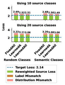
Figure 2: Transforms optimized using Eq. 3 produce a better bound than obtained by naively chosen transforms, primarily due to decreased distribution mismatch. We observe that the presence of random vs semantically related source classes has a limited impact on the bound.

We consider the transferability of a ResNet-18 model trained with Imagenet as the source and CIFAR10 as the target. We compare the cross-entropy loss on CIFAR10 obtained after linear finetuning with the predicted transferability obtained from the upper bound in Theorem 3. We show how different transform parameters affect our upper bound in Fig. 2. We test two settings. In the first setting, we select data from 10 random classes or 10 classes that are semantically related to the labels of CIFAR10 from Imagenet [15] and use them in our task transfer analysis (See App. D). With these we evaluate the bound, by fixing all transform parameters (FixedAll: $A$ is set to the Identity matrix, $B$ is a random permutation matrix, $D$ is set to the source prior), learning only $A$ (LearnedA: $A$ is optimized by solving Eq. 3 while $B,C$ are same as in FixedAll), and learning all the transforms (LearnedAll). The top part of Fig. 2 shows that for FixedAll, the presence of semantically related classes in the source data does not provide any advantage in terms of the bound compared to the presence of unrelated classes due to a lack of correct class-wise matching (via $B$) leading to a higher Wasserstein distance. The bound becomes significantly better (decreases by $\sim$ 0.2 from FixAll to LearnedA) when the feature transform $A$ is learned showing its advantage at decreasing the Wasserstein distance. Finally, learning all the transforms produces the best upper bound with both random and semantically chosen classes.

In the second setting, we select data from 20 classes from Imagenet by selecting either 20 random classes or 10 random and 10 semantically related classes. This setting allows us to analyze transferability when the source task has more classes than the target (for FixedAll and LearnedA, we fix $B$ to match two source classes entirely to a single target class.). In all cases, we observe that the upper bound becomes larger compared to our previous setting due to the increase of the reweighted source loss as learning a 20-way classifier is more challenging than learning a 10-way classifier, especially with the Lipschitz constraint. Despite this, just learning the transform $A$ (LearnedA) produces a better upper bound. The bound is further improved by learning all the transformations. Fig. 5 (in the Appendix) shows that by learning $C$ the optimization prefers to retain the data from 10 of the 20 classes reducing the reweighted source loss.

Based on these insights we find that selecting the same number of classes as that present in the target task and learning only the transform $A$ keeping $B,C$ fixed to a random permutation matrix and prior of the source can achieve a smaller upper bound. Thus, we use this setup for all our other experiments. Additional experiments demonstrating the effectiveness of learning the transformations by solving Eq. 3, for different datasets, are present in App. C.1.2.

4.3 Impact of task relatedness on transferability

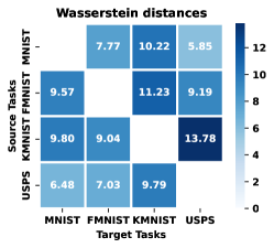
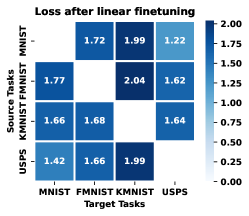
Figure 3: Task relatedness measured by $W_{d}(P_{S^{\prime\prime\prime}},P_{T})$ correlates strongly with transferability (i.e., target loss). Related tasks such as (MNIST, USPS) transfer better than (MNIST, KMNIST).

Here we evaluate how transferability is affected by the differences in the source tasks used for transfer. We consider a setup with convolutional neural networks trained using various character recognition tasks such as MNIST, Fashion-MNIST (FMNIST) [47], KMNIST [11], and USPS. We compute the pairwise transferability of these networks to other tasks. The results in Fig. 3 show that for a particular target task, the source task that achieves the smallest residual Wasserstein distance after task transfer (i.e. smallest $W_{d}(P_{S^{\prime\prime\prime}},P_{T})$) also achieves the smallest loss. For example, MNIST is the best source task to be used to transfer to USPS and vice-versa. This is intuitive since both datasets contain digits and the encoder trained for digits from the MNIST dataset, maps the corresponding digits from the USPS dataset close to MNIST images. Moreover, the data/classifier of MNIST can be easily transformed to explain the performance of USPS as seen by small $W_{d}(P_{S^{\prime\prime\prime}},P_{T})$. Similarly, when the Wasserstein distance of a target task to different source tasks is high, the fine-tuning loss also remains high (for ex. when the target task is KMNIST).

We also observe that Wasserstein distance plays a major role in explaining the variability in the upper bound to transferability for different target tasks while keeping the source task fixed as shown in Fig. 6 (in the Appendix). We further demonstrate the effect of task relatedness on transferability on a sentence classification problem in App. C.2.2. Our results in Fig. 8 and 10 (in the Appendix) again show that transferability improves when the source and target tasks are related as measured by the residual Wasserstein distance. Thus, task relatedness measured in terms of the residual Wasserstein distance between the transformed source and target distribution is correlated well with empirical transferability for different tasks across different applications.

4.4 Large-scale evaluation with various architectures/training methods/datasets

Here we demonstrate the effectiveness of the proposed upper bound and our optimization for task transfer at predicting transferability for the state-of-the-art pre-trained models. We consider pre-trained classifiers with architectures such as Vision Transformers (ViT) [17], ResNet-18/50 [21] trained with different pretraining methods including supervised training [21], adversarial training [38], SimCLR [8], MoCo [20], SwAV [7], CLIP [35], and MAE [19]. We consider a wide range of target datasets including, CIFAR10/100 [23], Aircraft [27], Pets [33] and DTD [10]. Additionally, we create two subsets of CIFAR100 with the first 25 (small) and 50 (medium) classes. We provide the details of these models, training methods, and datasets in App. D.

For this experiment, we consider the source task to be Imagenet [15] and use our optimization to transfer the source data along with the classifier learned on Imagenet for predicting transferability. The results of this experiment are shown in Fig. 4 and 9 (in the Appendix) which show that regardless of the pretraining algorithm and the model architecture of the pre-trained classifier, our bound predicts transferability effectively and achieves a small gap to empirical transferability. This shows that our upper bound is not vacuous and can explain why transfer learning is successful with large pre-trained classifiers. In Fig. 4 and 9, we show the contribution of individual terms in our upper bound and show that the label mismatch term only has a small contribution when $B$ matches source classes confidently to the target classes (i.e. a source class is fully matched to a single target class and is not partially matched to two or more classes). Our experiments show that when the source and target tasks have fewer classes learning $h_{S}$ is easier and the contribution of the reweighted source loss term is relatively small but this loss increases as the number of classes increases (especially, in the presence of the gradient penalty term used while learning $h_{S}$ and $h_{T}$). Moreover, the Wasserstein distance term becomes larger when pre-trained models have a larger representation space (e.g., ResNet-18/ViT-B16 have a 512-dimensional representation space whereas ResNet50 models have 2048-dimensional space). Having a larger representation space makes the computation of Wasserstein distance difficult and hence learning $A$ to reduce it becomes challenging. Nonetheless, our optimization finds a solution that consistently produces a small gap to empirical transferability. Additionally, we present results on the sentence classification problem in App. C.3.2 which are consistent with our findings on the image classification problem described here.

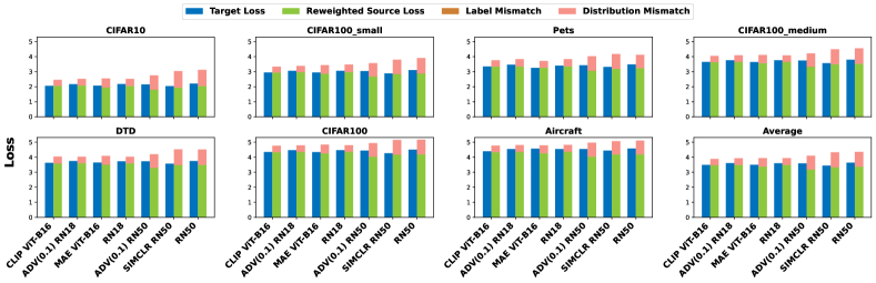
Figure 4: Transferability predicted by our analysis consistently achieves a small gap to empirical transferability for state-of-the-art large pre-trained models trained with various architectures/pretraining methods/datasets.

5 Discussion and conclusion

In this work, we analyzed transfer learning with linear fine-tuning by transforming the source distribution and the classifier to match those of the target task. We proved a bound on transferability which is a sum of three terms namely, reweighted source loss, label mismatch, and distribution mismatch. We also proposed an optimization problem to learn the task transfer effectively and using large-scale experiments demonstrated that our theoretical results can consistently explain transferability for various tasks and models pre-trained with different architectures/training methods.

While the task transfer analysis effectively explains transferability it is limited to linear fine-tuning with Lipschitz weights and cross-entropy loss. Thus, extending this work to a more general setting including the development of training methods to make models more transferable and providing an explanation of full fine-tuning are crucial problems that require further research and are topics of future works.

6 Acknowledgments

This work was supported by the NSF EPSCoR-Louisiana Materials Design Alliance (LAMDA) program #OIA-1946231.

We present the missing proofs of the theoretical results from Sec. 3 along with justifications for the classifiers ($h_{S^{\prime}},h_{S^{\prime\prime}},h_{S^{\prime\prime\prime}}$) as Corollaries in Appendix A followed by related work on learning in the presence of distribution shift with the same feature and label space in Appendix B. This is followed by additional experimental results including NLP classification tasks with large pretrained models in Appendix C. We conclude in Appendix D with details of the experiments and datasets used.

Appendix A Proofs for Sec. 3

A.1 Analysis of the task transfer model (Sec. 3.1)

A.1.1 Prior transform $(S\rightarrow S^{\prime})$

Lemma 1.

Let $C:=\left[\frac{P_{S^{\prime}}(y)}{P_{S}(y)}\right]_{y=1}^{|\mathcal{Y}_{S}|}$ be a vector of probability ratios and the classifier $h_{S^{\prime}}(z):=h_{S}(z)$, then $\mathbb{E}_{P_{S^{\prime}}(z,y)}[\ell(h_{S^{\prime}}(z),y)]=\mathbb{E}_{P_{S}(z,y)}[C(y)\ell(h_{S}(z),y)],\;$ for any loss function $\ell$.

Proof.

$$\mathbb{E}_{P_{S^{\prime}}(z,y)}[\ell(h_{S^{\prime}}(z),y)]=\mathbb{E}_{P_{S^{\prime}}(z,y)}[\ell(h_{S}(z),y)]=\sum_{y\in\mathcal{Y}_{S}}P_{S^{\prime}}(y)\mathbb{E}_{P_{S^{\prime}}(z|y)}[\ell(h_{S}(z),y)]$$

$$= \sum_{y\in\mathcal{Y}_{S}}\frac{P_{S}(y)}{P_{S}(y)}P_{S^{\prime}}(y)\mathbb{E}_{P_{S^{\prime}}(z|y)}[\ell(h_{S}(z),y)]=\sum_{y\in\mathcal{Y}_{S}}P_{S}(y)\mathbb{E}_{P_{S^{\prime}}(z|y)}[C(y)\ell(h_{S}(z),y)]$$

$$= \sum_{y\in\mathcal{Y}_{S}}P_{S}(y)\mathbb{E}_{P_{S}(z|y)}[C(y)\ell(h_{S}(z),y)]\quad(\mathrm{since}\;P_{S}(z|y)=P_{S^{\prime}}(z|y)\;\mathrm{by\;construction})$$

$$= \mathbb{E}_{P_{S}(z,y)}[C(y)\ell(h_{S}(z),y)].$$

∎

A.1.2 Label transform $(S^{\prime}\rightarrow S^{\prime\prime})$

Lemma 2.

Let $B$ be a $|\mathcal{Y}_{S}|\times|\mathcal{Y}_{T}|$ matrix such that $B_{ij}=P(y_{S^{\prime\prime}}=i|y_{S^{\prime}}=j)$ and $h_{S^{\prime\prime}}(z):=Bh_{S^{\prime}}(z)$. With the cross-entropy loss $\ell$, we have $\mathbb{E}_{P_{S^{\prime\prime}}(z,y)}[\ell(h_{S^{\prime\prime}}(z),y)]\leq\mathbb{E}_{P_{S^{\prime}}(z,y)}[\ell(h_{S^{\prime}}(z),y)]+{H}(\mathcal{Y}_{S^{\prime\prime}}|\mathcal{Y}_{S^{\prime}};B)$, where ${H}(\mathcal{Y}_{S^{\prime\prime}}|\mathcal{Y}_{S^{\prime}};B):=[-\sum_{y_{S^{\prime}}\in\mathcal{Y}_{S^{\prime}}}\sum_{y_{S^{\prime\prime}}\in\mathcal{Y}_{S^{\prime\prime}}}P_{S^{\prime}}(y_{S^{\prime}})B_{y_{S^{\prime\prime}},y_{S^{\prime}}}\log(B_{y_{S^{\prime\prime}},y_{S^{\prime}}})]$ is the conditional entropy.

Proof.

Note that $P(z):=P_{S^{\prime}}(z)=P_{S^{\prime\prime}}(z)$ by construction.

$$\mathbb{E}_{P_{S^{\prime\prime}}(z,y)}[\ell(h_{S^{\prime\prime}}(z),y)]=\mathbb{E}_{P(z,y^{\prime\prime})}[\ell(h_{S^{\prime\prime}}(z),y^{\prime\prime})]$$

$$= \mathbb{E}_{P(z)}\mathbb{E}_{P(y^{\prime\prime}|z)}[\ell(h_{S^{\prime\prime}}(z),y^{\prime\prime})]=\mathbb{E}_{P(z)}\sum_{y^{\prime\prime}}\sum_{y^{\prime}}P(y^{\prime\prime},y^{\prime}|z)[\ell(h_{S^{\prime\prime}}(z),y^{\prime\prime})]\;\;\;(\mathrm{since\;}\;y^{\prime}\in\mathcal{Y}_{S^{\prime}})$$

$$= \mathbb{E}_{P(z)}\mathbb{E}_{P(y^{\prime\prime},y^{\prime}|z)}[\ell(h_{S^{\prime\prime}}(z),y^{\prime\prime})]$$

$$= \mathbb{E}_{P(z)}\mathbb{E}_{P(y^{\prime}|z)}\mathbb{E}_{P(y^{\prime\prime}|y^{\prime})}[\ell(h_{S^{\prime\prime}}(z),y^{\prime\prime})]\;\;\;(\mathrm{since\;}P(y^{\prime\prime}|y^{\prime},z)=P(y^{\prime\prime}|y^{\prime}))$$

$$= \mathbb{E}_{P(z)}\mathbb{E}_{P(y^{\prime}|z)}[\sum_{y^{\prime\prime}\in\mathcal{Y}_{S^{\prime\prime}}}\ell(h_{S^{\prime\prime}}(z),y^{\prime\prime})B_{y^{\prime\prime},y^{\prime}}]\;\;\;(\mathrm{since\;}B_{y^{\prime\prime},y^{\prime}}=P(y^{\prime\prime}|y^{\prime}))$$

$$= \mathbb{E}_{P(z,y^{\prime})}[\sum_{y^{\prime\prime}\in\mathcal{Y}_{S^{\prime\prime}}}\ell(Bh_{S^{\prime}}(z),y^{\prime\prime})B_{y^{\prime\prime},y^{\prime}}].$$

Since the loss $\ell$ is the cross-entropy loss, we have

$$\ell(Bh_{S^{\prime}}(z),y^{\prime\prime}) = \ell(\sum_{j\in\mathcal{Y_{S^{\prime}}}}B_{y^{\prime\prime},j}h^{j}_{S^{\prime}}(z))=-\log(\sum_{j\in\mathcal{Y_{S^{\prime}}}}B_{y^{\prime\prime},j}h^{j}_{S^{\prime}}(z))$$

$$\leq -\log(B_{y^{\prime\prime},y^{\prime}}h^{y^{\prime}}_{S^{\prime}}(z))=-\log(B_{y^{\prime\prime},y^{\prime}})-\log(h^{y^{\prime}}_{S^{\prime}}(z)).$$

Therefore, we have

$$\mathbb{E}_{P_{S^{\prime\prime}}(z,y)}[\ell(h_{S^{\prime\prime}}(z),y)]$$

$$= \mathbb{E}_{P(z,y^{\prime})}[\sum_{y^{\prime\prime}\in\mathcal{Y}_{S^{\prime\prime}}}\ell(Bh_{S^{\prime}}(z),y^{\prime\prime})B_{y^{\prime\prime},y^{\prime}}]$$

$$\leq -\mathbb{E}_{P(z,y^{\prime})}[\sum_{y^{\prime\prime}\in\mathcal{Y}_{S^{\prime\prime}}}B_{y^{\prime\prime},y^{\prime}}\left(\log(B_{y^{\prime\prime},y^{\prime}})+\log(h^{y^{\prime}}_{S^{\prime}}(z))\right)]$$

$$= -\mathbb{E}_{P(z,y^{\prime})}[\sum_{y^{\prime\prime}\in\mathcal{Y}_{S^{\prime\prime}}}B_{y^{\prime\prime},y^{\prime}}\log(B_{y^{\prime\prime},y^{\prime}})]-\mathbb{E}_{P(z,y^{\prime})}[\sum_{y^{\prime\prime}\in\mathcal{Y}_{S^{\prime\prime}}}B_{y^{\prime\prime},y^{\prime}}\log(h^{y^{\prime}}_{S^{\prime}}(z))]$$

$$= -\mathbb{E}_{P(z,y^{\prime})}[\sum_{y^{\prime\prime}\in\mathcal{Y}_{S^{\prime\prime}}}B_{y^{\prime\prime},y^{\prime}}\log(B_{y^{\prime\prime},y^{\prime}})]+\mathbb{E}_{P(z,y^{\prime})}[-\log(h^{y^{\prime}}_{S^{\prime}}(z))\sum_{y^{\prime\prime}\in\mathcal{Y}_{S^{\prime\prime}}}B_{y^{\prime\prime},y^{\prime}}]$$

$$= -\mathbb{E}_{P(z,y^{\prime})}[\sum_{y^{\prime\prime}\in\mathcal{Y}_{S^{\prime\prime}}}B_{y^{\prime\prime},y^{\prime}}\log(B_{y^{\prime\prime},y^{\prime}})]+\mathbb{E}_{P(z,y^{\prime})}[-\log(h^{y^{\prime}}_{S^{\prime}}(z))]$$

$$= \mathbb{E}_{P(z,y^{\prime})}[-\sum_{y^{\prime\prime}\in\mathcal{Y}_{S^{\prime\prime}}}B_{y^{\prime\prime},y^{\prime}}\log(B_{y^{\prime\prime},y^{\prime}})]+\mathbb{E}_{P(z,y^{\prime})}[\ell(h_{S^{\prime}}(z),y^{\prime})]$$

$$= \mathbb{E}_{P(y^{\prime})}\mathbb{E}_{P_{S^{\prime}}(z|y^{\prime})}[-\sum_{y^{\prime\prime}\in\mathcal{Y}_{S^{\prime\prime}}}B_{y^{\prime\prime},y^{\prime}}\log(B_{y^{\prime\prime},y^{\prime}})]+\mathbb{E}_{P(z,y^{\prime})}[\ell(h_{S^{\prime}}(z),y^{\prime})]$$

$$= [-\sum_{y^{\prime}\in\mathcal{Y}_{S^{\prime}}}\sum_{y^{\prime\prime}\in\mathcal{Y}_{S^{\prime\prime}}}P(y^{\prime})B_{y^{\prime\prime},y^{\prime}}\log(B_{y^{\prime\prime},y^{\prime}})]+\mathbb{E}_{P(z,y^{\prime})}[\ell(h_{S^{\prime}}(z),y^{\prime})]$$

$$= H(\mathcal{Y}_{S^{\prime\prime}}|\mathcal{Y}_{S^{\prime}};B)+\mathbb{E}_{P_{S^{\prime}}(z,y)}[\ell(h_{S^{\prime}}(z),y)].$$

∎

Corollary 2 below, shows the conditions under which the optimal softmax classifier for the domain $S^{\prime}$ remains optimal for the domain $S^{\prime\prime}$, justifying our choice of classifier change from $S^{\prime}$ to $S^{\prime\prime}$.

Corollary 2.

Let $|\mathcal{Y}_{S^{\prime\prime}}|=|\mathcal{Y}_{S^{\prime}}|$, $B$ be a $|\mathcal{Y}_{S}|\times|\mathcal{Y}_{T}|$ permutation matrix and $h_{S^{\prime}}$ be the optimal softmax classifier for $S^{\prime}$ and $y_{S^{\prime\prime}}:=\sigma(y_{S^{\prime}}):=\arg\max_{y\in\mathcal{Y}_{S^{\prime\prime}}}(Be(y_{S^{\prime}}))_{y}$ then under the assumptions of Lemma 2, $h_{S^{\prime\prime}}(z):=Bh_{S^{\prime}}(z)$ is the optimal softmax classifier for $S^{\prime\prime}$.

Proof.

Since $y_{S^{\prime\prime}}:=\sigma(y_{S^{\prime}}):=\arg\max_{y\in\mathcal{Y}_{T}}(Be(y_{S^{\prime}}))_{y}$ we have

$$\mathbb{E}_{P_{S^{\prime\prime}}}[\ell(h_{S^{\prime\prime}}(z),y_{S^{\prime\prime}})] = \mathbb{E}_{P(z,y^{\prime\prime})}[\ell(Bh_{S^{\prime}}(z),y^{\prime\prime})]=\sum_{y^{\prime\prime}\in\mathcal{Y}_{S^{\prime\prime}}}P(y^{\prime\prime})\mathbb{E}_{P(z|y^{\prime\prime})}[\ell(Bh_{S^{\prime}}(z),y^{\prime\prime})]$$

$$= \sum_{y^{\prime}\in\mathcal{Y}_{S^{\prime}}}P(\sigma(y^{\prime}))\mathbb{E}_{P(z|\sigma(y^{\prime}))}[\ell(Bh_{S^{\prime}}(z),\sigma(y^{\prime}))]$$

$$= \sum_{y^{\prime}\in\mathcal{Y}_{S^{\prime}}}P(y^{\prime})\mathbb{E}_{P(z|y^{\prime})}[\ell(h_{S^{\prime}}(z),y^{\prime})]=\mathbb{E}_{P_{S^{\prime}}}[\ell(h_{S^{\prime}}(z),y_{S^{\prime}})].$$

The second last equality follows due to the symmetry of cross-entropy loss, i.e., $\ell(h,y)=-\log h_{y}=-\log Bh_{\sigma(y)}=l(Bh,\sigma(y))$.

With $h_{S^{\prime\prime}}(z)=Bh_{S^{\prime}}(z)$, $\arg\min_{h_{S^{\prime}}}\mathbb{E}_{P_{S^{\prime}}}[\ell(h_{S^{\prime}}(z),y_{S^{\prime}})]=\arg\min_{h_{S^{\prime\prime}}}\mathbb{E}_{P_{S^{\prime\prime}}}[\ell(h_{S^{\prime\prime}}(z),y_{S^{\prime\prime}})]$. Hence $h_{S^{\prime\prime}}(z)=Bh_{S^{\prime}}(z)$ is the optimal softmax classifier for $S^{\prime\prime}$, if $h_{S^{\prime}}$ is optimal for $S^{\prime}$. ∎

A.1.3 Feature transform $(S^{\prime\prime}\rightarrow S^{\prime\prime\prime})$

Lemma 3.

Let $A:\mathcal{Z}\to\mathcal{Z}$ be an invertible map of features and the classifier $h_{S^{\prime\prime\prime}}(z_{S^{\prime\prime\prime}}):=h_{S^{\prime\prime}}(A^{-1}(z_{S^{\prime\prime\prime}}))$. Then $\mathbb{E}_{P_{S^{\prime\prime\prime}}(z,y)}[\ell(h_{S^{\prime\prime\prime}}(z),y)]=\mathbb{E}_{P_{S^{\prime\prime}}(z,y)}[\ell(h_{S^{\prime\prime}}(z),y)]$.

Proof.

$\mathbb{E}_{P_{S^{\prime\prime\prime}}(z,y)}[\ell(h_{S^{\prime\prime\prime}}(z),y)]=\mathbb{E}_{P_{S^{\prime\prime\prime}}(z,y)}[\ell(h_{S^{\prime\prime}}(A^{-1}(z)),y)]=\mathbb{E}_{P_{S^{\prime\prime}}(z,y)}[\ell(h_{S^{\prime\prime}}(z),y)].$ ∎

Our Corollary 3 below shows that the optimal softmax classifier for domain $S^{\prime\prime}$ remains optimal for domain $S^{\prime\prime\prime}$ too.

Corollary 3.

Let $h_{S^{\prime\prime}}$ be the optimal softmax classifier in domain $S^{\prime\prime}$ then under the assumptions of Lemma 3, $h_{S^{\prime\prime\prime}}(x_{S^{\prime\prime\prime}})=h_{S^{\prime\prime}}(A^{-1}(x_{S^{\prime\prime\prime}}))$ is the optimal softmax classifier in domain $S^{\prime\prime\prime}$.

Proof.

When $h_{S^{\prime\prime\prime}}(x_{S^{\prime\prime\prime}})=h_{S^{\prime\prime}}(A^{-1}(x_{S^{\prime\prime\prime}}))$, $\arg\min_{h_{S^{\prime\prime}}}\mathbb{E}_{P_{S^{\prime\prime}}(z,y)}[\ell(h_{S^{\prime\prime}}(z),y)]=\arg\min_{h_{S^{\prime\prime\prime}}}\mathbb{E}_{P_{S^{\prime\prime\prime}}(z,y)}[\ell(h_{S^{\prime\prime\prime}}(z),y)]$ by Lemma 3, hence if $h_{S^{\prime\prime}}$ is optimal for $S^{\prime\prime}$ then so is $h_{S^{\prime\prime\prime}}$ for the domain $S^{\prime\prime\prime}$. ∎

A.1.4 Three transforms combined $(S\rightarrow S^{\prime\prime\prime})$

Theorem 1.

Under the assumptions of Lemmas 1, 2, 3 we have

$$\mathbb{E}_{P_{S^{\prime\prime\prime}}(z,y)}[\ell(h_{S^{\prime\prime\prime}}(z),y)]\leq\mathbb{E}_{P_{S}(z,y)}[C(y)\ell(h_{S}(z),y)]+{H}(\mathcal{Y}_{T}|\mathcal{Y}_{S^{\prime}};B).$$

Proof.

$$\mathbb{E}_{P_{S^{\prime\prime\prime}}(z,y)}[\ell(h_{S^{\prime\prime\prime}}(z),y)] = \mathbb{E}_{P_{S^{\prime\prime}}(z,y)}[\ell(h_{S^{\prime\prime}}(z),y)]\;\mathrm{(Lemma~{}\ref{lemma:feature_transform})}$$

$$\leq \mathbb{E}_{P_{S^{\prime}}(z,y)}[\ell(h_{S^{\prime}}(z),y)]+{H}(\mathcal{Y}_{T}|\mathcal{Y}_{S^{\prime}};B)\;\mathrm{(Lemma~{}\ref{lemma:label_transform},\;since}\;\mathcal{Y}_{S^{\prime\prime\prime}}=\mathcal{Y}_{T})$$

$$= \mathbb{E}_{P_{S}(z,y)}[C(y)\ell(h_{S}(z),y)]+{H}(\mathcal{Y}_{T}|\mathcal{Y}_{S^{\prime}};B)\;\mathrm{(Lemma~{}\ref{lemma:prior_transform})}.$$

∎

Corollary 1.

Let $|Y_{S^{\prime\prime\prime}}|=|Y_{S}|$, $B:\Delta_{S^{\prime}}\rightarrow\Delta_{S^{\prime\prime}}$ be a permutation matrix and $y_{S^{\prime\prime}}:=\sigma(y_{S^{\prime}}):=\arg\max_{y\in\mathcal{Y}_{S^{\prime\prime}}}(Be(y_{S^{\prime}}))_{y}$ then under the assumptions of Lemmas 1, 2, and  3 we have

$$\mathbb{E}_{P_{S^{\prime\prime\prime}}(z,y)}[\ell(h_{S^{\prime\prime\prime}}(z),y)]=\mathbb{E}_{P_{S}(z,y)}[C(y)\ell(h_{S}(z),y)]$$

Proof.

Since $y_{S^{\prime\prime}}:=\sigma(y_{S^{\prime}}):=\arg\max_{y\in\mathcal{Y}_{T}}(Be(y_{S^{\prime}}))_{y}$ we have

$$\mathbb{E}_{P_{S^{\prime\prime}}}[\ell(h_{S^{\prime\prime}}(z),y_{S^{\prime\prime}})] = \mathbb{E}_{P(z,y^{\prime\prime})}[\ell(Bh_{S^{\prime}}(z),y^{\prime\prime})]=\sum_{y^{\prime\prime}\in\mathcal{Y}_{S^{\prime\prime}}}P(y^{\prime\prime})\mathbb{E}_{P(z|y^{\prime\prime})}[\ell(Bh_{S^{\prime}}(z),y^{\prime\prime})]$$

$$= \sum_{y^{\prime}\in\mathcal{Y}_{S^{\prime}}}P(\sigma(y^{\prime}))\mathbb{E}_{P(z|\sigma(y^{\prime}))}[\ell(Bh_{S^{\prime}}(z),\sigma(y^{\prime}))]$$

$$= \sum_{y^{\prime}\in\mathcal{Y}_{S^{\prime}}}P(y^{\prime})\mathbb{E}_{P(z|y^{\prime})}[\ell(h_{S^{\prime}}(z),y^{\prime})]=\mathbb{E}_{P_{S^{\prime}}(z,y)}[\ell(h_{S^{\prime}}(z),y)].$$

Therefore, we have

$$\mathbb{E}_{P_{S^{\prime\prime\prime}}(z,y)}[\ell(h_{S^{\prime\prime\prime}}(z),y)] = \mathbb{E}_{P_{S^{\prime\prime}}(z,y)}[\ell(h_{S^{\prime\prime}}(z),y)]\;\mathrm{(Lemma~{}\ref{lemma:feature_transform})}$$

$$= \mathbb{E}_{P_{S^{\prime}}(z,y)}[\ell(h_{S^{\prime}}(z),y)]\;\mathrm{(from\;above)}$$

$$= \mathbb{E}_{P_{S}(z,y)}[C(y)\ell(h_{S}(z),y)]\;\mathrm{(Lemma~{}\ref{lemma:prior_transform})}.$$

∎

A.2 Distribution mismatch between $S^{\prime\prime\prime}$ and $T$ (Sec. 3.2)

Lemma 4.

Let $R$ and $Q$ be two distributions in $\mathcal{Z}\times\mathcal{Y}$ with the same prior $P_{R}(y=i)=P_{Q}(y=i)=P(y=i)$. With the distance $d((z,y),(z^{\prime},y^{\prime})):=\|z-z^{\prime}\|_{2}+\infty\cdot 1_{y\neq y^{\prime}}$, where $z,z^{\prime}\in\mathcal{Z}$ and $y,y^{\prime}\in\mathcal{Y}$, we have $W_{d}(P_{R},P_{Q})=\sum_{y}W_{\|\cdot\|_{2}}(P_{R}(z|y),P_{Q}(z|y))P(y)$.

Proof.

Let $\omega_{y}^{\ast}$ denote the optimal coupling for the conditional distributions $(P_{R}(z|y),P_{Q}(z|y))$ for $y\in\mathcal{Y}$ and $\pi^{\ast}$ denote the the optimal coupling for the joint distributions $(P_{R}(z,y),P_{Q}(z,y))$. Then, under the definition of our base distance $d$, $\pi^{\ast}((z,y),(z^{\prime},y^{\prime}))=0$ when $y\neq y^{\prime}$ i.e. no mass from the distribution $R$ belonging to class $y$ can be moved to the classes $y^{\prime}\neq y$ of the distribution $Q$ when the class priors of $R$ and $Q$ are the same. Moreover, since $\sum_{ij}(\omega^{\ast}_{y})_{ij}=1$ and $\sum_{\{i,j:y_{i}=y^{\prime}_{j}=k\}}\pi^{\ast}_{ij}=P(y=k)$ for $k\in\mathcal{Y}$ we have $\pi^{*}((z,y),(z^{\prime},y^{\prime}))=\omega^{*}_{y}(z,z^{\prime})P(y)1_{y=y^{\prime}}$ for every $y,y^{\prime}\in\mathcal{Y}$.

Then, we can show that the total Wasserstein distance between the joint distributions can be expressed as the sum of conditional Wasserstein distances, as follows

$$W_{d}(P_{R}(z,y),P_{Q}(z,y))$$

$$= \sum_{y,y^{\prime}}\int\pi^{\ast}((z,y),(z^{\prime},y^{\prime}))d((z,y),(z^{\prime},y^{\prime}))dzdz^{\prime}$$

$$= \sum_{y,y^{\prime}}\int\pi^{\ast}((z,y),(z^{\prime},y^{\prime}))(\|z-z^{\prime}\|_{2}+\infty\cdot 1_{y\neq y^{\prime}})dzdz^{\prime}$$

$$= \sum_{y,y^{\prime}}\int\omega^{*}_{y}(z,z^{\prime})P(y)1_{y=y^{\prime}}(\|z-z^{\prime}\|_{2}+\infty\cdot 1_{y\neq y^{\prime}})dzdz^{\prime}$$

$$= \sum_{y,y^{\prime}}\int\omega^{*}_{y}(z,z^{\prime})P(y)1_{y=y^{\prime}}\|z-z^{\prime}\|_{2}dzdz^{\prime}\;\;(\mathrm{since}\;1_{y=y^{\prime}}\cdot 1_{y\neq y^{\prime}}=0)$$

$$= \sum_{y,y^{\prime}}P(y)1_{y=y^{\prime}}\int\omega^{*}_{y}(z,z^{\prime})\|z-z^{\prime}\|_{2}dzdz^{\prime}$$

$$= \sum_{y}P(y)\int\omega^{*}_{y}(z,z^{\prime})\|z-z^{\prime}\|_{2}dzdz^{\prime}$$

$$= \sum_{y}W_{\|\cdot\|_{2}}(P_{R}(z|y),P_{Q}(z|y))P(y).$$

∎

Theorem 2.

Let the distributions $T$ and $S^{\prime\prime\prime}$ be defined on the same domain $\mathcal{Z}\times\mathcal{Y}$ and assumption 1 holds, then for the base distance $d((z,y),(z^{\prime},y^{\prime}))=\|z-z^{\prime}\|_{2}+\infty\cdot 1_{y\neq y^{\prime}}$ we have,

$$\mathbb{E}_{P_{T}(z,y)}[\ell(z,y)]-\mathbb{E}_{P_{S^{\prime\prime\prime}}(z,y)}[\ell(z,y)]\leq\tau\;W_{d}(P_{S^{\prime\prime\prime}},P_{T};A,B).$$

Proof.

$$\mathbb{E}_{P_{T}(z,y)}[\ell(z,y)]-\mathbb{E}_{P_{S^{\prime\prime\prime}}(z,y)}[\ell(z,y)]$$

$$= \mathbb{E}_{P_{T}(y)}\mathbb{E}_{P_{T}(z|y)}[\ell(z,y)]-\mathbb{E}_{P_{S^{\prime\prime\prime}}(y)}\mathbb{E}_{P_{S^{\prime\prime\prime}}(z|y)}[\ell(z,y)]$$

$$= \mathbb{E}_{P_{T}(y)}[\mathbb{E}_{P_{T}(z|y)}[\ell(z,y)]-\mathbb{E}_{P_{S^{\prime\prime\prime}}(z|y)}[\ell(z,y)]]\;(\mathrm{since\;}P_{T}(y)=P_{S^{\prime\prime\prime}}(y))$$

$$\leq \mathbb{E}_{P_{T}(y)}[\sup_{\ell^{\prime}\in\tau-Lipschitz}\mathbb{E}_{P_{T}(z|y)}[\ell^{\prime}(z,y)]-\mathbb{E}_{P_{S^{\prime\prime\prime}}(z|y)}[\ell^{\prime}(z,y)]]$$

$$= \mathbb{E}_{P_{T}(y)}[\tau\;W_{\|\cdot\|_{2}}(P_{T}(z|y),P_{S^{\prime\prime\prime}}(z|y))]\;(\mathrm{Kantorovich-Rubinstein\;duality})$$

$$= \tau\;W_{d}(P_{S^{\prime\prime\prime}},P_{T};A,B)\;(\mathrm{Lemma~{}\ref{lemma:WD_same}}).$$

∎

A.3 Final bound (Sec. 3.3)

Theorem  3.

Let $\ell$ be the cross entropy loss then under the assumptions of Theorems 1 and 2 we have,

$$\mathbb{E}_{P_{T}(z,y)}[\ell(h_{T}(z),y)] \leq \mathbb{E}_{P_{S}(z,y)}[C(y)\ell(h_{S}(z),y)]+{H}(\mathcal{Y}_{T}|\mathcal{Y}_{S^{\prime}};B)+\tau\;W_{d}(P_{S^{\prime\prime\prime}},P_{T};A,B)$$

Proof.

$$\mathbb{E}_{P_{T}(z,y)}[\ell(h_{T}(z),y)]\leq\mathbb{E}_{P_{T}(z,y)}[\ell(h_{S^{\prime\prime\prime}}(z),y)]\;(\mathrm{Gap\;due\;to\;classifier\;difference})$$

$$\leq \mathbb{E}_{P_{S^{\prime\prime\prime}}(z,y)}[\ell(h_{S^{\prime\prime\prime}}(z),y)]+\tau\;W_{d}(S^{\prime\prime\prime},T;A,B)\;(\mathrm{Theorem~{}\ref{theorem:dist_shift}})$$

$$\leq \mathbb{E}_{P_{S}(z,y)}[C(y)\ell(h_{S}(z),y)]+{H}(\mathcal{Y}_{T}|\mathcal{Y}_{S^{\prime}};B)+\tau\;W_{d}(S^{\prime\prime\prime},T;A,B)\;(\mathrm{Theorem~{}\ref{theorem:accuracy_transfer}}).$$

∎

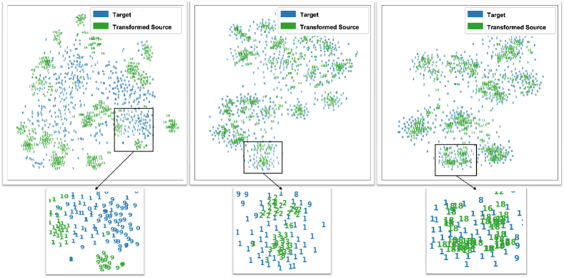
Figure 5: (Best viewed in color.) t-SNE visualizations of the effect of various transformations on the bound in Theorem 3 when data from 20 randomly selected classes from Imagenet are used to transfer to CIFAR-10. When all transformations are fixed (FixedAll, left) the distance between the distribution $S^{\prime\prime\prime}$ (transformed source) and $T$ is high explaining the large upper bound. Learning just the transformation $A$ using the algorithm proposed in Sec. 4.1 significantly reduces the distance between $S^{\prime\prime\prime}$ and $T$ leading to a tighter upper bound (center). Learning all the transformations further improves the matching (right). Especially, learning $B$ and $D$ change the class priors of the source so that the same number of classes from the source are used for matching as those present in the target. This is evident from the right plot where only 10 unique source clusters are visible compared to 20 in the center plot, with fixed D. Moreover, the zoomed-in portion shows that for the center figure two classes from the source (green 2 and 3) match with class 1 (blue) of the target whereas a single class from the source (green 18) matches class 1 (blue) of the target in the right figure.

Appendix B Distributional divergence-based analyses of learning with distribution shifts (under same feature and label sets)

Here we review some of the previous works which analyzed the problem of learning under distribution shifts in terms of distributional divergences such as the Wasserstein distance. These analyses apply when the feature and label spaces remain the same between the original and the shifted distribution.

Early works [5, 41, 28] showed that the performance on a shifted distribution (target domain) can be estimated in terms of the performance of the source domain and the distance between the two domains’ marginal distributions and labeling functions. Specifically, [5] showed that that

$$\mathcal{E}_{T}(h,f_{T})\leq\mathcal{E}_{S}(h,f_{S})+d_{1}(P_{S},P_{T})+\min\{\mathbb{E}_{P_{S}}[|f_{S}(z)-f_{T}(z)|],\mathbb{E}_{\mathcal{D}_{T}}[|f_{S}(z)-f_{T}(z)|]\},$$

where $d_{1}$ denotes the total variation distance, $f:\mathcal{Z}\rightarrow[0,1]$ denotes the labeling function, $h:\mathcal{Z}\rightarrow\{0,1\}$ denotes the hypothesis and $\mathcal{E}_{P}(h,f):=\mathbb{E}_{z\sim P}[|h(z)-f(z)|]$ denote the risk of the hypothesis $h$. A follow up work [41], showed a similar result using type-1 Wasserstein distance for all $K-$Lipschitz continuous hypotheses i.e.,

$$\mathcal{E}_{T}(h,f_{T})\leq\mathcal{E}_{S}(h,f_{S})+2K\cdot W_{1}(P_{S},P_{T})+\lambda,$$

where $\lambda$ is the combined error of the ideal hypothesis $h^{\ast}$ that minimizes the combined error $\mathcal{E}_{S}(h,f_{S})+\mathcal{E}_{T}(h,f_{T})$. Another recent work [25] used a target transformation-based approach and Wasserstein distance to quantify learning in the presence of data and label shifts. Other works [24, 40] also presented an analysis based on Wasserstein distance to understand how the accuracy of smoothed classifies and robustness change in the presence of distribution shifts. Compared to these works the bound proposed in Theorem 2 considers cross-entropy loss (which is a popular choice of the loss function in the classification setting) and uses a joint feature and labels Wasserstein distance rather than only marginal Wasserstein distance. These differences make the bound proposed in Theorem 2 useful in the analysis of transfer learning than those proposed in previous works when we have access to labeled target domain data.

Appendix C Additional experiments

C.1 Additional results for the effectiveness of the proposed optimization (Sec. 4.2)

C.1.1 Visualization of the transformed data via t-SNE for various settings in Sec. 4.2

In this section, we use the setting considered in Sec. 4.2 where we consider 20 randomly selected classes from Imagenet as the source and consider the transfer to CIFAR-10. We plot the results of using different transformations using t-SNE to show how various transformations affect the upper bound in Theorem 3. Our results in Fig. 5(left) show that when no transformations are learned (FixedAll), the 20 random source classes do not overlap with the 10 target classes leading to an increased Wasserstein distance which in turn leads to a larger upper bound. By learning the transformation $A$ (LearnedA), Fig. 5(center) shows a significantly better alignment between the classes of the source and target which leads to a decreased Wasserstein distance and hence a tighter upper bound. Moreover, by learning all the transformations (LearnedAll), Fig. 5(right) shows that not only do the distributions align well but also the prior of the source is changed to only keep 10 source classes to match the prior of the target distribution providing a further improvement in the upper bound. This clearly shows the effectiveness of our proposed optimization algorithm in learning various transformations to minimize the upper bound.

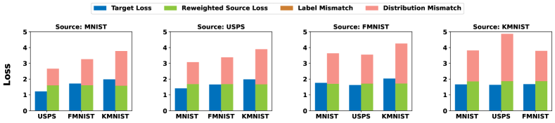
Figure 6: Decomposition of the bound in Theorem 3 into its three components illustrates that the distribution mismatch term explains the variability in the loss after linear fine-tuning. Similar tasks such as USPS and MNIST have the smallest loss after fine-tuning and also have the smallest residual Wasserstein distance, $W_{d}(S^{\prime\prime\prime},T)$, after learning the transformations using our optimization.

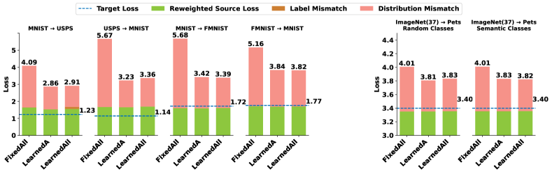
Figure 7: Comparison of using various transformations on the upper bound for different datasets. For all datasets learning the transformation by solving the optimization problem in Eq. 3 leads to a significantly tighter upper bound on the loss incurred after linear fine-tuning.

C.1.2 Additional experiments for transferring in different settings/datasets

Here we extend the experiment presented in Sec. 4.2 to the Pets dataset. Specifically, we select data from 37 random and semantically related (list in App. D) source classes from Imagenet and use them to transfer to the Pets dataset. Results for this experiment are present in Fig. 7 (2 right-most plots). Consistent with the results presented in the main paper, we find that learning just the transformation $A$ produces a significantly better upper bound than when all transformations are fixed. Moreover, learning all the transformations produces a similar or slightly better result than learning only $A$ in this setting. Lastly, the presence of semantically related or random classes in the source does not produce a significant difference in terms of the bound.

Next, we evaluate the effectiveness of the optimization on datasets such as MNIST, FMNIST, and USPS. For these datasets, we first train a convolutional neural network model on the data from the source task and then perform linear finetuning using the data from the target task. Similar to the previous experiments, the results in Fig. 7 (first 4 plots) show that when the transformations are fixed, the gap between the loss on the target data after linear fine-tuning and the upper bound is large. Learning the transformations by solving the proposed optimization in Eq. 3 reduces this gap significantly. For the experiment with the source as MNIST and target as USPS and vice-versa, we additionally compare our results to a setting where only $A$ is learned and $B$ is set to an identity matrix (rather than a permutation matrix, as used in LearnedA setting). This matrix $B$ contains the correct matching between the labels of the source and target. We find that the upper bound obtained when $B$ is fixed to identity is only marginally better than the case when $B$ is a random permutation or is learned through solving our optimization problem. Specifically, with $B$ learned through our optimization the upper bound improves by 0.15 for the MNIST$\rightarrow$USPS task and by 0.3 for the USPS$\rightarrow$MNIST task. As expected the primary reason for the decrease in the upper bound comes from the reduced Wasserstein distance $W_{d}(S^{\prime\prime\prime},T)$ and the label mismatch term. While the upper bound improves slightly when the ideal matching between the labels is known, such a mapping may not be known when the labels of the tasks are not related such as for FMNIST and MNIST. Moreover, due to the difficulty of the optimization problem (different label associations producing similar upper bounds) recovering the true association between the labels could be hard. Similar to [1], a more complicated version of the label distance that depends on the features of the data could be used to remedy this problem, but analyzing the compatibility of such a label distance with the proposed bound requires further research.

C.2 Additional results for the impact of task relatedness on transferability (Sec. 4.3)

C.2.1 Additional results for image classification

Here we provide details of the experiment presented in Sec. 4.3 about the effect of task relatedness on the transferability after linear fine-tuning. Similar to the results presented in Fig. 3 of the main paper the results in Fig. 6 show that when the source and the target tasks are related then both the loss after linear fine-tuning and our bound are small as in the case when the source is MNIST and target is USPS or vice versa. When the target tasks are unrelated to the source data then both the loss after linear fine-tuning and our bound remain the same regardless of the chosen source data. For example, when the target task is KMNIST, using MNIST, USPS or FMNIST produces the same loss and the upper bound. Lastly, for any particular source, Fig. 6 shows that the bound only differs because of the differences in the distribution mismatch term which measures $W_{d}(S^{\prime\prime\prime},T)$. This shows that when the distribution mismatch can be minimized, both the empirical and predicted transferability improve, demonstrating transfer between related source and target tasks is both easier and explainable.

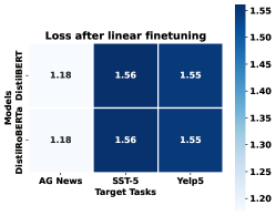
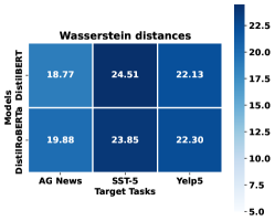
Figure 8: Task relatedness measured by $W_{d}(P_{S^{\prime\prime\prime}},P_{T})$ correlates with transferability (i.e., target loss). A target task related to DBPedia such as AG News achieves a smaller loss and a smaller residual Wasserstein distance compared to less-related tasks such as SST-5 and Yelp5.

C.2.2 Results for NLP sentence classification task

In this section, we use sentence classification NLP task to further demonstrate the effect of task relatedness on transferability and the proposed upper bound. For this experiment, we first fine-tune the entire DistilBERT [39] and DistilRoBERTa [26] models distilled on English Wikipedia and Toronto Book Corpus, and OpenAI’s WebText dataset, respectively, using a subsample of 10,000 points from the DBPedia dataset. We then use these fine-tuned models to evaluate the transferability to AG news, SST-5, and Yelp datasets. The results in Fig. 8 show that the loss after linear fine-tuning on AG News is the smallest among the three datasets. This coincides with the Wasserstein distance obtained after learning the transformations which explains why transfer to AG News is more successful compared to other datasets. This observation is reasonable, especially considering that both DBPedia and AG News have structured information. Moreover, since DBPedia is related to Wikipedia, the terms and entities appearing in AG News are more related to those appearing in DBPedia in comparison to terms/entities appearing in SST-5 and Yelp which consist of movie reviews and reviews collected from Yelp.

For our experiments, in this section, we follow a similar setting of fixing $B$ to be a random permutation matrix, $C$ to the prior of the source, and only learn the transformation $A$. We sample 10,000 points from DBPedia belonging to the same number of classes as those present in the target task (for ex., for AG News we sample data from 4 randomly selected classes of DBPedia) and use this data as the source data to train $h_{S}$ with gradient norm penalty ($\tau$=0.02). All experiments are run for 3 random seeds and average results are reported in Fig. 8.

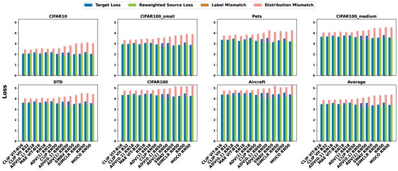
Figure 9: Additional results for comparison of empirical versus predicted transferability for large pre-trained models. Our upper bound proposed in Theorem 3 consistently achieves a small gap to empirical transferability obtained after linear fine-tuning.

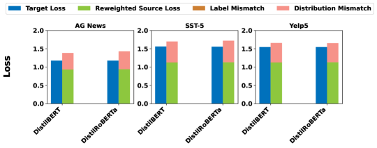
Figure 10: Transferability predicted by our analysis consistently achieves a small gap to empirical transferability even for NLP classification tasks (AG News, SST-5, Yelp5) using DistilBERT and DistilRoBERTa as pre-trained models which are fully fine-tuned with DBPedia.

C.3 Additional results for predicting transferability using large pre-trained models (Sec. 4.4)

C.3.1 Additional results image classification

Here we present additional results on computer vision classification tasks of predicting transferability through the bound proposed in Theorem 3 which were omitted in the main paper due to space limitation. Consistent with the results shown in Fig. 4 of the main paper, from the results in Fig. 9 we observe that there is a small gap between the loss after linear fine-tuning and the bound for models trained with various pre-training methods and architectures. Moreover, the bound is tighter for models trained with architectures that have a smaller representation space such as ResNet18 and ViT-B-16 which have 512-dimensional representation space. This is attributed to the difficulty of optimizing the Wasserstein distance in higher dimensional representation space.

C.3.2 Results for NLP sentence classification task

In addition to vision tasks, we also evaluate the effectiveness of our optimization at minimizing the upper bound for NLP classification tasks. Similar to Sec. C.2.2, we focus on the task of sentence classification here. For this experiment, we fine-tune the entire DistilBERT [39] and DistilRoBERTa [26] models distilled on English Wikipedia and Toronto Book Corpus, and OpenAI’s WebText dataset, respectively, using a subsample of 10,000 points from the DBPedia dataset. Using the encoder of this new model, we linearly fine-tune using the data from the target tasks as well as use our optimization to learn the transformations to minimize the upper bound. The results present in Fig. 10, show that our bound consistently achieves a small gap to the loss after linear fine-tuning. These results show that task transfer can effectively explain transferability across a wide range of tasks.

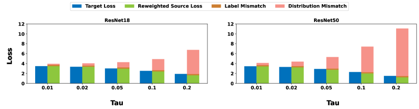
Figure 11: Trade-off between the fine-tuning loss and the bound of Theorem 3 as a function of $\tau$. Increasing the value of $\tau$ leads to a decreased fine-tuning loss but leads to an increase in the bound proposed in Theorem 3 leading to a lowered explainability of transfer learning.

C.4 Lipschitz constraints for linear finetuning

C.4.1 Implementing softmax classification with $\tau$-Lipschitz loss

To use the bound Theorem. 3, it is required that the loss be $\tau$-Lipschitz continuous w.r.t. $z$ in a bounded input domain $\mathcal{Z}$. To enforce this, while learning the weights of the softmax classifier (aka linear fine-tuning) for the source or the target, we add the gradient norm penalty as used in previous works [41, 2] and solve the following optimization problem

$$\min_{h}\frac{1}{N}\sum_{i}\left[\ell(h(z_{i}),y_{i})+\rho\max_{y}\max\{0,\|\nabla_{z}\ell(h(z_{i}),y)\|-\tau\}\right]\;\;\;(\rho\approx 10^{5})$$

where $\ell(h(z),y)=-w_{y}^{T}z+\log\sum_{j}e^{w_{j}^{T}z}$.

C.4.2 Trade-off between empirical and predicted transferability

Constraining the Lipschitz coefficient of the classifier increases both the target and the source loss since the hypothesis set is being restricted. The smaller the $\tau$ is, the larger the loss becomes. On the other hand, the smaller $\tau$ makes the distribution mismatch term in Theorem 3 also smaller. Since the bound is the sum of the source loss and the distribution mismatch (and label mismatch), there is a trade-off determined by the value of $\tau$. We illustrate the effect of the values of $\tau$ on the empirical and predicted transferability. As mentioned previously, we train both the classifier for the source $h_{S}$ and the target $h_{T}$ with an additional penalty on the gradient norm to make them $\tau$-Lipschitz. In Fig. 11, we present results of varying the value of $\tau$ for the transfer to the Pets dataset with Imagenet as the source. For this experiment, we selected 37 random classes from Imagenet and only learned the transform $A$ by keeping $B$ fixed to a random permutation and $C$ fixed to the uniform prior over source classes. We observe that the performance of linear fine-tuning degrades as we decrease the value of $\tau$ but explainability through the bound improves since the distribution mismatch (dependent on $\tau$) decreases in the bound. However, making $\tau$ too small is not preferable since it leads to an increase in the first term of the bound making the overall bound increase. For our experiments, we use $\tau=$ 0.02 since it doesn’t decrease the performance of fine-tuning significantly and leads to a small gap between empirical and predicted transferability.

Appendix D Details of the experiments

All codes are written in Python using Tensorflow/Pytorch and were run on an Intel(R) Xeon(R) Platinum 8358 CPU with 200 GB of RAM and an Nvidia A10 GPU. Implementation and hyperparameters are described below. Our codes can be found at https://github.com/akshaymehra24/TaskTransferAnalysis.

D.1 Dataset details

In our work, we used the standard image classification benchmark datasets along with standard natural language processing datasets.

Aircraft [27]: consists of 10,000 aircraft images belonging to 100 classes.

CIFAR-10/100 [23]: These datasets contain 60,000 images belonging to 10/100 categories.

DTD[10]: consists of 5,640 textural images belonging to 47 categories.

Fashion MNIST [47]: consists of 70,000 grayscale images belonging to 10 categories.

Pets [33]: consists of 7049 images of Cats and Dogs spread across 37 categories.

Imagenet [15]: consists of 1.1 million images belonging to 1000 categories.

Yelp [49]: consists of 650,000 training and 50,000 test examples belonging to 5 classes.

Stanford Sentiment Treebank (SST-5) [49]: consists of 8,544 training and 2,210 test samples belonging to 5 classes.

AG News [49]: consists of 120,000 training and 7,600 test examples belonging to 4 classes

DBPedia [49]: consists of 560,000 training and 70,000 test examples belonging to 14 classes

D.2 Semantically similar classes for CIFAR-10 and Pets from Imagenet

For our experiments with CIFAR-10 in Sec. 4.2, we selected the following semantically similar classes from Imagenet, {airliner, minivan, cock, tabby cat, ox, chihuahua, bullfrog, sorrel, submarine, fire engine}. For our experiments with the Pets dataset in App. C.1.2, we selected the following classes for Dogs {boston bull, miniature schnauzer, giant schnauzer, standard schnauzer, scotch terrier, chrysanthemum dog, silky terrier, a soft-coated wheaten terrier, west Highland white terrier, lhasa, lat-coated retriever, curly-coated retriever, golden retriever, labrador retriever, chesapeake bay retriever, german short-haired pointer, vizsla, hungarian pointer, english setter, irish setter, gordon setter, brittany spaniel, clumber, english springer, welsh springer spaniel, cocker spaniel} and the following for Cats {tabby, tiger cat, persian cat, siamese cat, egyptian cat, cougar, lynx, leopard, snow leopard, jaguar, lion, tiger}. Since some species of Cats and Dogs present in the Pets dataset are not present in Imagenet, we select broadly related classes for our experiments.

D.3 Additional experimental details

In our experiments, in Sec. 4.4, we used pre-trained models available from Pytorch for ResNet18/50, along with publically available pre-trained models provided in the official repositories of each training method. For each experiment, we subsample data from the Imagenet dataset belonging to the same number of classes as those present in the target dataset and use this data to train the linear layer on top of the representations extracted from the pre-trained model along with a gradient norm penalty. To speed up the experiments, we use only 10,000 points from the subsample of Imagenet for training the linear classifier and computing the transfer. For evaluation, we use a similar subsample of the validation dataset of Imagenet containing all the samples belonging to the subsampled classes. Fine-tuning on this dataset takes about 0.05 seconds per epoch for the task of transfer from Imagenet to Pets with the ResNet-18 model (we run the finetuning for a total of 5000 epochs).

Along with training the linear classifiers with a gradient norm penalty, we standardize the features extracted from the pre-trained models to remove their mean (along each axis) and make them have a unit standard deviation (along each axis). While standardizing the features do not have a significant impact on the loss of the classifiers, including it makes it easier to match the distributions of the source and target data after transformations. Since our optimization problem transforms the source distribution to match the distribution of the target by solving the optimization problem in Eq. 3 by working on mini-batches, it is important that the size of the batch be greater than the dimension of the representation space of the pre-trained encoder. For example, for ResNet18 models which have a representation dimension of 512, we use a batch size of 1000 and for ResNet50 models which have a representation dimension of 2048, we use a batch size of 2500. Having a smaller batch size than the dimension could lead to a noisy gradient since for that batch the transformation can achieve a perfect matching, which may not generalize to data from other batches or unseen test data.

While computing the transformations, we apply the same augmentation (re-sizing and center cropping)/normalization to the training data as those applied to the test data. Along with this, we extract the features of the training and test data from the pre-trained model once and use these to train the linear layer. We note that this is done to save the computation time and better results could be obtained by allowing for extracting features after data augmentation for every batch.

Finally, for our experiments in Sec. 4.3, the encoders are trained end-to-end on the source task. This is in contrast to our other experiments where the encoders are pre-trained and data from the source task is only used for linear fine-tuning. This is done since there are no pre-trained models available for MNIST-type tasks considered in this section and training a model on these datasets is relatively easy and cheap. Using these models, task relatedness is evaluated by fine-tuning a linear layer using the data from the target task as well as the transformations are computed by solving Eq. 3. We used $\tau=$0.2 here. We run the experiments with 3 random seeds and report the average results.

References

- [1] David Alvarez-Melis and Nicolo Fusi. Geometric dataset distances via optimal transport. arXiv preprint arXiv:2002.02923, 2020.
- [2] Martin Arjovsky, Soumith Chintala, and Léon Bottou. Wasserstein generative adversarial networks. In International conference on machine learning, pages 214–223. PMLR, 2017.
- [3] Yajie Bao, Yang Li, Shao-Lun Huang, Lin Zhang, Lizhong Zheng, Amir Zamir, and Leonidas Guibas. An information-theoretic approach to transferability in task transfer learning. In 2019 IEEE International Conference on Image Processing (ICIP), pages 2309–2313, 2019.
- [4] Shai Ben-David, John Blitzer, Koby Crammer, Alex Kulesza, Fernando Pereira, and Jennifer Wortman Vaughan. A theory of learning from different domains. Machine learning, 79(1):151–175, 2010.
- [5] Shai Ben-David, John Blitzer, Koby Crammer, Fernando Pereira, et al. Analysis of representations for domain adaptation. Advances in neural information processing systems, 19:137, 2007.
- [6] Shai Ben-David and Reba Schuller. Exploiting task relatedness for multiple task learning. In Learning theory and kernel machines, pages 567–580. Springer, 2003.
- [7] Mathilde Caron, Ishan Misra, Julien Mairal, Priya Goyal, Piotr Bojanowski, and Armand Joulin. Unsupervised learning of visual features by contrasting cluster assignments. Advances in neural information processing systems, 33:9912–9924, 2020.
- [8] Ting Chen, Simon Kornblith, Mohammad Norouzi, and Geoffrey Hinton. A simple framework for contrastive learning of visual representations. In International conference on machine learning, pages 1597–1607. PMLR, 2020.
- [9] Xinlei Chen, Saining Xie, and Kaiming He. An empirical study of training self-supervised vision transformers, 2021.
- [10] Mircea Cimpoi, Subhransu Maji, Iasonas Kokkinos, Sammy Mohamed, and Andrea Vedaldi. Describing textures in the wild. In Proceedings of the IEEE conference on computer vision and pattern recognition, pages 3606–3613, 2014.
- [11] Tarin Clanuwat, Mikel Bober-Irizar, Asanobu Kitamoto, Alex Lamb, Kazuaki Yamamoto, and David Ha. Deep learning for classical japanese literature. arXiv preprint arXiv:1812.01718, 2018.
- [12] Nicolas Courty, Rémi Flamary, Amaury Habrard, and Alain Rakotomamonjy. Joint distribution optimal transportation for domain adaptation. Advances in neural information processing systems, 30, 2017.
- [13] Jifeng Dai, Yi Li, Kaiming He, and Jian Sun. R-fcn: Object detection via region-based fully convolutional networks. Advances in neural information processing systems, 29, 2016.
- [14] Bharath Bhushan Damodaran, Benjamin Kellenberger, Rémi Flamary, Devis Tuia, and Nicolas Courty. Deepjdot: Deep joint distribution optimal transport for unsupervised domain adaptation. In Proceedings of the European Conference on Computer Vision (ECCV), pages 447–463, 2018.
- [15] Jia Deng, Wei Dong, Richard Socher, Li-Jia Li, Kai Li, and Li Fei-Fei. Imagenet: A large-scale hierarchical image database. In 2009 IEEE conference on computer vision and pattern recognition, pages 248–255. Ieee, 2009.
- [16] Jacob Devlin, Ming-Wei Chang, Kenton Lee, and Kristina Toutanova. Bert: Pre-training of deep bidirectional transformers for language understanding, 2019.
- [17] Alexey Dosovitskiy, Lucas Beyer, Alexander Kolesnikov, Dirk Weissenborn, Xiaohua Zhai, Thomas Unterthiner, Mostafa Dehghani, Matthias Minderer, Georg Heigold, Sylvain Gelly, Jakob Uszkoreit, and Neil Houlsby. An image is worth 16x16 words: Transformers for image recognition at scale, 2021.
- [18] Remi Flamary, Nicolas Courty, Alexandre Gramfort, Mokhtar Z Alaya, Aureie Boisbunon, Stanislas Chambon, Laetitia Chapel, Adrien Corenflos, Kilian Fatras, Nemo Fournier, et al. Pot: Python optimal transport. The Journal of Machine Learning Research, 22(1):3571–3578, 2021.
- [19] Kaiming He, Xinlei Chen, Saining Xie, Yanghao Li, Piotr Dollár, and Ross Girshick. Masked autoencoders are scalable vision learners. In Proceedings of the IEEE/CVF Conference on Computer Vision and Pattern Recognition, pages 16000–16009, 2022.
- [20] Kaiming He, Haoqi Fan, Yuxin Wu, Saining Xie, and Ross Girshick. Momentum contrast for unsupervised visual representation learning. In Proceedings of the IEEE/CVF conference on computer vision and pattern recognition, pages 9729–9738, 2020.
- [21] Kaiming He, Xiangyu Zhang, Shaoqing Ren, and Jian Sun. Deep residual learning for image recognition, 2015.
- [22] Long-Kai Huang, Ying Wei, Yu Rong, Qiang Yang, and Junzhou Huang. Frustratingly easy transferability estimation, 2022.
- [23] Alex Krizhevsky, Geoffrey Hinton, et al. Learning multiple layers of features from tiny images. ., 2009.
- [24] Aounon Kumar, Alexander Levine, Tom Goldstein, and Soheil Feizi. Certifying model accuracy under distribution shifts. arXiv preprint arXiv:2201.12440, 2022.
- [25] Trung Le, Tuan Nguyen, Nhat Ho, Hung Bui, and Dinh Phung. Lamda: Label matching deep domain adaptation. In International Conference on Machine Learning, pages 6043–6054. PMLR, 2021.
- [26] Yinhan Liu, Myle Ott, Naman Goyal, Jingfei Du, Mandar Joshi, Danqi Chen, Omer Levy, Mike Lewis, Luke Zettlemoyer, and Veselin Stoyanov. Roberta: A robustly optimized bert pretraining approach. arXiv preprint arXiv:1907.11692, 2019.
- [27] Subhransu Maji, Esa Rahtu, Juho Kannala, Matthew Blaschko, and Andrea Vedaldi. Fine-grained visual classification of aircraft. arXiv preprint arXiv:1306.5151, 2013.
- [28] Yishay Mansour, Mehryar Mohri, and Afshin Rostamizadeh. Domain adaptation: Learning bounds and algorithms. arXiv preprint arXiv:0902.3430, 2009.
- [29] Akshay Mehra, Bhavya Kailkhura, Pin-Yu Chen, and Jihun Hamm. Understanding the limits of unsupervised domain adaptation via data poisoning. In Thirty-Fifth Conference on Neural Information Processing Systems, 2021.
- [30] Akshay Mehra, Bhavya Kailkhura, Pin-Yu Chen, and Jihun Hamm. Do domain generalization methods generalize well? In NeurIPS ML Safety Workshop, 2022.
- [31] Cuong V. Nguyen, Tal Hassner, Matthias Seeger, and Cedric Archambeau. Leep: A new measure to evaluate transferability of learned representations, 2020.
- [32] Sinno Jialin Pan and Qiang Yang. A survey on transfer learning. IEEE Transactions on Knowledge and Data Engineering, 22(10):1345–1359, 2010.
- [33] Omkar M Parkhi, Andrea Vedaldi, Andrew Zisserman, and CV Jawahar. Cats and dogs. In 2012 IEEE conference on computer vision and pattern recognition, pages 3498–3505. IEEE, 2012.
- [34] Gabriel Peyré, Marco Cuturi, et al. Computational optimal transport: With applications to data science. Foundations and Trends® in Machine Learning, 11(5-6):355–607, 2019.
- [35] Alec Radford, Jong Wook Kim, Chris Hallacy, Aditya Ramesh, Gabriel Goh, Sandhini Agarwal, Girish Sastry, Amanda Askell, Pamela Mishkin, Jack Clark, et al. Learning transferable visual models from natural language supervision. In International conference on machine learning, pages 8748–8763. PMLR, 2021.
- [36] Shaoqing Ren, Kaiming He, Ross Girshick, and Jian Sun. Faster r-cnn: Towards real-time object detection with region proposal networks. Advances in neural information processing systems, 28, 2015.
- [37] Sebastian Ruder. An overview of multi-task learning in deep neural networks. arXiv preprint arXiv:1706.05098, 2017.
- [38] Hadi Salman, Andrew Ilyas, Logan Engstrom, Ashish Kapoor, and Aleksander Madry. Do adversarially robust imagenet models transfer better? Advances in Neural Information Processing Systems, 33:3533–3545, 2020.
- [39] Victor Sanh, Lysandre Debut, Julien Chaumond, and Thomas Wolf. Distilbert, a distilled version of bert: smaller, faster, cheaper and lighter, 2020.
- [40] Vikash Sehwag, Saeed Mahloujifar, Tinashe Handina, Sihui Dai, Chong Xiang, Mung Chiang, and Prateek Mittal. Robust learning meets generative models: Can proxy distributions improve adversarial robustness? arXiv preprint arXiv:2104.09425, 2021.
- [41] Jian Shen, Yanru Qu, Weinan Zhang, and Yong Yu. Wasserstein distance guided representation learning for domain adaptation. In Thirty-Second AAAI Conference on Artificial Intelligence, 2018.
- [42] Aman Sinha, Hongseok Namkoong, Riccardo Volpi, and John Duchi. Certifying some distributional robustness with principled adversarial training. arXiv preprint arXiv:1710.10571, 2017.
- [43] Yang Tan, Yang Li, and Shao-Lun Huang. Otce: A transferability metric for cross-domain cross-task representations, 2021.
- [44] Anh T. Tran, Cuong V. Nguyen, and Tal Hassner. Transferability and hardness of supervised classification tasks, 2019.
- [45] Cédric Villani. Optimal transport: old and new, volume 338. Springer, 2009.
- [46] Karl Weiss, Taghi M Khoshgoftaar, and Dingding Wang. A survey of transfer learning. Journal of Big Data, 3(1):9, May 2016.
- [47] Han Xiao, Kashif Rasul, and Roland Vollgraf. Fashion-mnist: a novel image dataset for benchmarking machine learning algorithms. arXiv preprint arXiv:1708.07747, 2017.
- [48] Kaichao You, Yong Liu, Jianmin Wang, and Mingsheng Long. Logme: Practical assessment of pre-trained models for transfer learning, 2021.
- [49] Xiang Zhang, Junbo Zhao, and Yann LeCun. Character-level convolutional networks for text classification. Advances in neural information processing systems, 28, 2015.