Abstract

We present a full space-time numerical solution of the advection-diffusion equation using a continuous Galerkin finite element method. The Galerkin/least-square method is employed to ensure stability of the discrete variational problem. In the full space-time formulation, time is considered another dimension, and the time derivative is interpreted as an additional advection term of the field variable. We derive a priori error estimates and illustrate spatio-temporal convergence with several numerical examples. We also derive a posteriori error estimates, which coupled with adaptive space-time mesh refinement provide efficient and accurate solutions. The accuracy of the space-time solutions is illustrated against analytical solutions as well as against numerical solutions using a conventional time-marching algorithm.

1 Introduction

Numerically solving a transient (or evolution) problem characterized by a partial differential equation (PDE) requires that the continuous problem be discretized in space and time. The standard way to deal with this dual discretization, is to use a suitable time-marching algorithm coupled with some form of spatial discretization such as the finite difference method (FDM), the finite element method (FEM), the finite volume method (FVM) or the more recent isogeometric analysis (IgA). In most cases, the time marching algorithms themselves are based on (a variant of) finite difference methods and are used along with the above mentioned spatial discretizations. Generally speaking, these approaches consider the spatio-temporal domain over which the solution is desired as a product of a spatial domain with a temporal domain, with independent discretization and analysis of each of these components.

An alternative strategy to “time-marching” is to discretize and solve for the full “space-time” domain together. Any combination of spatial and temporal discretization can be used – for instance, finite difference schemes in both space and time; or FEM in space and FDM in time; or FEM in both space and time. In particular, in the context of FEM, this constitutes a second type of “space-time” formulation, where finite element formulation is used in both space and time, but time marching is not employed. A major attraction for formulating a problem in space-time is the possibility of improved parallel performance. The idea of parallelism in both space and time builds on a rich history of parallel time integration [3, 4, 5]. We refer to [6, 7] for a review of such methods.

The finite element community has a history of considering solutions to time dependent PDEs in space-time. The earliest references to space-time formulations go back to the mid 1980’s. Babuska and co-workers [8, 9] developed $h-p$ versions of finite element method in space along with p and $h-p$ versions of approximations in time for parabolic problems. Around the same time, Hughes and Hulbert formulated a space-time finite element method for elastodynamics problem [10] and general hyperbolic problems [11] using time-discontinuous Galerkin method. Recently, there has been increasing interest in revisiting this problem given access to larger computational resources [12, 13, 14]. In this work, we tackle two key aspects associated with solving evolution equations in space-time – stability and computational cost. We focus on a particular family of PDE’s, specifically the time dependent advection-diffusion equations, with the time dependent diffusion equation as a special case (when the advection term goes to zero).

Stability of the discrete space-time formulation: When solving parabolic equations through space-time methods, the question of stability of the ensuing discrete system becomes important. As mentioned earlier, in a sequential setting the time derivative term is treated separately during temporal discretization. But when the advection-diffusion equation is formulated in space-time (i.e. time is considered another dimension, like the rest of the spatial dimensions), the time evolution term (first order derivative with respect to time) can be mathematically seen as an “advection in time dimension” term and can be grouped with the other spatial first derivatives in the equation [15]. This identification is mathematically consistent since all the first order derivatives, irrespective of whether they are spatial or temporal, have a sense of “directionality” attached to them (the actual direction is determined by the sign of their coefficients). Mathematically then, the problem can be seen as a “generalized advection-diffusion equation” in space-time, except, there is no diffusion term associated with the time dimension. This type of equation, when solved through the standard Galerkin method, can suffer from a lack of stability and end up with spurious oscillations [16, 17]. Andreev and Mollet analyzed the stability of space-time FEM discretizations of abstract linear parabolic evolution equations [18, 19]. Steinbach also analyzed the stability of the heat equation in space-time setting and derived error bounds using unstructured space-time finite elements [20]. In 2017, Langer et al. [12] used a time-upwind type Petrov-Galerkin basis function similar to the streamline diffusion method, to solve the heat equation in space-time moving domains. There is a large body of literature available that deals with treating non self-adjoint operators through finite element method [16, 21, 22, 23, 24], a review of which can be found in [25]. In this work, we build upon this body of work and ensure stability of the discrete variational form by using a Galerkin/least squares (GLS) approach. We show that GLS provides stability to the discrete space-time problem and derive a priori error bounds in the discrete norm associated with the bilinear form.

Reducing computational cost via space-time adaptivity: Clearly, a space-time formulation adds one more dimension to concurrently discretize. A 2D problem needs a 3D mesh and a 3D problem needs a 4D mesh. Thus the number of degrees of freedom in the resulting linear system can become significantly larger than the corresponding sequential problem. Prior research has shown that this increased computational cost is ideally suited to sustained parallelism [5, 27, 28, 29, 30, 31, 12, 13, 14]. Additional efficiencies can be accessed by making efficient use of adaptive mesh refinement (AMR) in space-time [32, 13, 14, 33, 34]. To this end, we mathematically derive a residual-based a posteriori error indicator which can be used to estimate elementwise errors. This enables us to leverage the benefits of AMR in a space-time setting which render very accurate solution to the diffusion problem and the advection-diffusion problems considered here.

The rest of the content of this paper is organized as follows. In Section 2, we introduce the mathematical formulation of the problem. We formulate the continuous and the discrete problems and state the relevant function spaces. We then prove the stability of the discrete bilinear form and then derive a priori and a posteriori error estimates. Then in Section 3, we present numerical examples that validate the theoretical results of Section 2 and also demonstrate the advantages of using adaptive mesh refinement in space-time analysis. Finally in Section 4 we draw conclusions and make some comments about future research directions.

2 Mathematical Formulation

2.1 The time-dependent linear advection-diffusion equation

Consider a bounded space domain $U\in\mathbb{R}^{n},n=1,2,3$ with Lipschitz continuous boundary $\partial U$ and a bounded time interval $I_{{}_{T}}=(0,T]\in\mathbb{R^{+}}$. We define the space-time domain as the Cartesian product of the two as $\Omega=U\times I_{{}_{T}}=U\times(0,T]$. The overall boundary of this space-time domain is defined as $\Gamma=\partial\Omega$. This “overall boundary” is the union of the “spatial boundaries” and the “time boundaries”. The spatial domain boundary is denoted by $\Gamma_{{}_{S}}=\partial U\times(0,T]$; whereas the time boundaries are denoted by $\Gamma_{{}_{0}}=\bar{U}\times\{0\}$ and $\Gamma_{{}_{T}}=\bar{U}\times\{T\}$ which are the initial and final time boundaries respectively. The closure of the space-time domain is $\bar{\Omega}=\Omega\cup\Gamma_{{}_{S}}\cup\Gamma_{{}_{0}}$. The advection-diffusion equation can then be written for the scalar function $u:\Omega\rightarrow\mathbb{R}$ as:

$$\mathscr{L}u =f\quad\textrm{in}\quad\Omega,$$ (1a)

$$u =0\quad\textrm{on}\quad\Gamma_{{}_{S}},$$ (1b)

$$u(\cdot,t_{0}) =u_{0}\quad\textrm{on}\quad\Gamma_{0},$$ (1c)

with

$$\mathscr{L}u=u_{t}+{\underline{a}}\cdot\underline{{\nabla}\mkern-4.0mu}\mkern 4.0muu-\underline{{\nabla}\mkern-4.0mu}\mkern 4.0mu\cdot(\kappa\underline{{\nabla}\mkern-4.0mu}\mkern 4.0muu),$$ (2)

where $u_{t}$ denotes $\frac{\partial u}{\partial t}$ and $f:\Omega\rightarrow\mathbb{R}$ is a smooth forcing function. The diffusivity $\kappa$ is positive and does not depend on $u$. Dirichlet boundary conditions are imposed on the boundary $\Gamma_{{}_{S}}$. Also, $\underline{{\nabla}\mkern-4.0mu}\mkern 4.0mu$ is the gradient operator in the space $\mathbb{R}^{n}$, i.e., for example in 3 dimensions,

$$\underline{{\nabla}\mkern-4.0mu}\mkern 4.0mu\equiv\left(\frac{\partial}{\partial x},\frac{\partial}{\partial y},\frac{\partial}{\partial z}\right).$$ (3)

We further define the space-time gradient operator $\underline{\widetilde{\nabla}\mkern-4.0mu}\mkern 4.0mu$ as:

$$\underline{\widetilde{\nabla}\mkern-4.0mu}\mkern 4.0mu\equiv\left(\frac{\partial}{\partial x},\frac{\partial}{\partial y},\frac{\partial}{\partial z},\frac{\partial}{\partial t}\right).$$ (4)

The operator in (2) can also be interpreted as $(\frac{\partial}{\partial t}+L)u$, where $L={\underline{a}}\cdot\underline{{\nabla}\mkern-4.0mu}\mkern 4.0mu-\underline{{\nabla}\mkern-4.0mu}\mkern 4.0mu\cdot(\kappa\underline{{\nabla}\mkern-4.0mu}\mkern 4.0mu)$. Since $L$ itself is elliptic and there is no second-order derivative with respect to time, it follows that the operator $(\frac{\partial}{\partial t}+L)$ is strictly parabolic. Such equations are typically solved with a method of lines discretization, by solving a series of discrete equations sequentially. At each “time-step”, the solution is assumed to be a function of the spatial variables only. In the context of the Galerkin methods, this spatial approximation takes the form of a (discrete) Sobolev space, e.g., the solution at the $i^{\text{th}}$ step, $u^{i}(x)\in H^{1}(U)$. But in this work, our focus will be coupled space-time formulation of the advection-diffusion equation where we approximate the solution in a Sobolev space defined on the full space-time domain (i.e., $u(x,t)\in H^{1}(\Omega)$). As alluded to in the introduction, this kind of problem formulation requires some form of stabilization. Here, the Galerkin/Least Squares method is used for this purpose.

When we add such stabilizing terms to the original variational problem, we essentially end up adding some numerical “diffusion” into the system. More importantly, perhaps, diffusion is introduced in the time direction as well, which is absent in the original parabolic equation. We show, in the results section, that careful design of stabilization ensures that this diffusion in the time direction is arbitrarily small. In essence, then, the equation becomes elliptic in the space-time domain. Anticipating such changes to the equation, we can cast this parabolic equation as a generalized elliptic equation as follows,

$$-\sum_{i=1}^{n+1}\sum_{j=1}^{n+1}\frac{\partial}{\partial x_{i}}\left(A_{ij}(x)\frac{\partial u}{\partial x_{j}}\right)+\sum_{i=1}^{n+1}B_{i}(x)\frac{\partial u}{\partial x_{i}}=f,$$ (5)

where $A_{ij}$ and $B_{i}$ are the components of $\underline{\underline{A}}\in\mathbb{R}^{(n+1)\times(n+1)}$ and $\underline{B}\in\mathbb{R}^{(n+1)}$; $n$ is the number of space dimensions and thus $(n+1)$ accounts for the inclusion of the time dimension.

We can recast (2) in this form (for $n=3$ dimensions), with $\underline{\underline{A}}$ and $\underline{B}$:

$$\underline{\underline{A}}=\begin{bmatrix}\kappa&0&0&0\\ 0&\kappa&0&0\\ 0&0&\kappa&0\\ 0&0&0&0\end{bmatrix},\qquad\underline{B}=\begin{bmatrix}b_{1}\\ b_{2}\\ b_{3}\\ 1\end{bmatrix},$$ (6)

where all off-diagonal entries as well as the last diagonal entry in ${\underline{\underline{A}}}$ are zero. After we finish the formulation with Galerkin/Least squares, we will eventually have a (arbitrarily small) positive real entry in the last diagonal term along with some non-zero term in the off-diagonals. Note that we have also assumed an isotropic diffusive medium, so the principal diffusivity values are the same in all directions. This assumption can be trivially relaxed. In the ${\underline{a}}$ vector, along with the spatial advection components, we have the “advection in time” component which has the value 1.

This equation can then be rewritten in a more compact form:

$$\left(-\underline{\widetilde{\nabla}\mkern-4.0mu}\mkern 4.0mu\cdot\underline{\underline{A}}\cdot\underline{\widetilde{\nabla}\mkern-4.0mu}\mkern 4.0mu+\underline{B}\cdot\underline{\widetilde{\nabla}\mkern-4.0mu}\mkern 4.0mu\right)u=f.$$ (7)

2.2 Variational problem and function spaces

If $u({\underline{x}},t)$ is the exact solution of equation (1), then we can write $u$ as

$$u({\underline{x}},t) =v({\underline{x}},t)+g({\underline{x}},t),$$ (8)

where,

$$v({\underline{x}},t) =0,\text{ when }{\underline{x}}\in\Gamma_{{}_{S}}\cup\Gamma_{{}_{0}}$$ (9)

and $g$ is some function in $V$ with the property:

$$g({\underline{x}},t) =\begin{cases}u_{0}({\underline{x}}),&\text{ when }{\underline{x}}\in\Gamma_{{}_{0}}\\ 0,&\text{ when }{\underline{x}}\in\Gamma_{{}_{S}}.\end{cases}$$ (10)

Substituting (8) into (1a), we have $\mathscr{L}v=f-\mathscr{L}g$. By defining the new right hand side as $F=f-\mathscr{L}g$, we can recast (1) as follows,

$$\mathscr{L}v =F\quad\textrm{in}\quad\Omega$$ (11a)

$$v =0\quad\textrm{on}\quad\Gamma_{{}_{S}}$$ (11b)

$$v({\underline{x}},t_{0}) =u_{0}\quad\textrm{on}\quad\Gamma_{0}$$ (11c)

Define the function space $V$ for the weak solution to (11) as,

$$V=\{v\in H^{1}(\Omega):v=0\textrm{ on }\Gamma_{0}\cup\Gamma_{s}\}$$ (12)

Then the variational problem for (11) is given by: find $v\in V$ such that

$$b(v,w)=l(w)\quad\forall w\in V,$$ (13)

where $b(v,w)=(\mathscr{L}v,w)$ and $l(w)$ are the bilinear and linear forms associated with the variational formulation of (11). They are defined as follows:

$$b(v,w) =\int_{\Omega}\left(v_{t}w+({\underline{a}}\cdot\underline{{\nabla}\mkern-4.0mu}\mkern 4.0muv)w+\kappa\underline{{\nabla}\mkern-4.0mu}\mkern 4.0muv\cdot\underline{{\nabla}\mkern-4.0mu}\mkern 4.0muw\right)d\Omega$$ (14a)

$$=(v_{t},w)+({\underline{a}}\cdot\underline{{\nabla}\mkern-4.0mu}\mkern 4.0muv,w)+(\kappa\underline{{\nabla}\mkern-4.0mu}\mkern 4.0muv,\underline{{\nabla}\mkern-4.0mu}\mkern 4.0muw)$$ (14b)

$$l(w) =\int_{\Omega}\left(Fw\right)d\Omega$$ (14c)

$$=(F,w),$$ (14d)

where $(\cdot,\cdot)$ denotes the $L^{2}$-inner product in the space-time domain $\Omega$, e.g., $(v,w)=\int_{\Omega}vw\text{ }d\Omega=\int_{0}^{T}\int_{U}vw\text{ }dUdt$.

2.3 Discrete variational problem

Define $\mathcal{K}_{h}$ as the partition of $\Omega$ into a finite number of non-overlapping (here, hexahedral) elements. For the finite element problem, we define the finite dimensional subspace $V_{h}\subset V$, which is defined as

$$V_{h}=\{v^{h}\in V:v^{h}|_{K}\in P_{m}(K),K\in\mathcal{K}_{h}\},$$ (15)

where $P_{m}(K)$ is the space of polynomial functions of degree less than or equal to $m$ in $K$. In this work, we consider $m=1$.

Solutions to equation (1) can exhibit numerical instabilities because the bilinear form $a(u,v)$ in equation (13) is not strongly coercive in $V_{u}$  [12]. This issue can be tackled by adding some amount of numerical diffusion in the time direction or by adding upwind type correction to the weighting functions  [12, 20]. But as can be expected, the difficulty increases when advection is present in the system. In what follows, we try to establish a stable variational form of the space-time advection-diffusion problem stated in (1) by applying the Galerkin/least square (GLS) method. The resulting discrete problem is stable and converges to the original PDE in the limit of the mesh size approaching zero.

An equation of the form $\mathscr{L}v=F$ can be cast into a least square minimization problem as

$$v=\operatorname*{arg\,min}_{w\in V}\|\mathscr{L}w-F\|^{2}.$$ (16)

The resulting Euler-Lagrange equation corresponding to this minimization problem is

$$\left(\mathscr{L}v,\mathscr{L}w\right)=\left(F,\mathscr{L}w\right).$$ (17)

In the GLS formulation, equation (17) is added to the original weighted equation (13). Therefore the GLS formulation for the equation $\mathscr{L}v=F$ reads as: find $v^{h}\in V_{h}$ such that,

$$(\mathscr{L}v^{h},w^{h})+\epsilon(\mathscr{L}v^{h},\mathscr{L}w^{h}) =(F,w^{h})+\epsilon(F,\mathscr{L}w^{h}),\quad\forall w^{h}\in V_{h},$$ (18)

$$\textrm{or,\qquad\quad}(\mathscr{L}v^{h},w^{h}+\epsilon\mathscr{L}w^{h}) =(F,w^{h}+\epsilon\mathscr{L}w^{h}),\quad\forall w^{h}\in V_{h},$$ (19)

where $\epsilon$ is a positive parameter to be chosen later. Thus the discrete variational problem with Galerkin–least-square stabilization reads as: find $v^{h}\in V_{h}$ such that

$$b^{h}(v^{h},w^{h})=l^{h}(w^{h})\quad\forall w^{h}\in V_{h},$$ (20)

where the discrete bilinear form $b^{h}(v^{h},w^{h})$ and linear form $l^{h}(w^{h})$ are as follows:

$$\begin{split}b^{h}(v^{h},w^{h})&=(v^{h}_{t},w^{h})+({\underline{a}}\cdot\underline{{\nabla}\mkern-4.0mu}\mkern 4.0muv^{h},w^{h})+(\kappa\underline{{\nabla}\mkern-4.0mu}\mkern 4.0muv^{h},\underline{{\nabla}\mkern-4.0mu}\mkern 4.0muw^{h})\\ &\quad+\epsilon(v^{h}_{t},w^{h}_{t})+\epsilon(v^{h}_{t},{\underline{a}}\cdot\underline{{\nabla}\mkern-4.0mu}\mkern 4.0muw^{h})+\epsilon(\underline{{\nabla}\mkern-4.0mu}\mkern 4.0muv^{h}_{t},\kappa\underline{{\nabla}\mkern-4.0mu}\mkern 4.0muw^{h})\\ &\quad+\epsilon({\underline{a}}\cdot\underline{{\nabla}\mkern-4.0mu}\mkern 4.0muv^{h},w^{h}_{t})+\epsilon({\underline{a}}\cdot\underline{{\nabla}\mkern-4.0mu}\mkern 4.0muv^{h},{\underline{a}}\cdot\underline{{\nabla}\mkern-4.0mu}\mkern 4.0muw^{h})-\epsilon(({\underline{a}}\cdot\underline{{\nabla}\mkern-4.0mu}\mkern 4.0muv^{h}),\underline{{\nabla}\mkern-4.0mu}\mkern 4.0mu\cdot(\kappa\underline{{\nabla}\mkern-4.0mu}\mkern 4.0muw^{h}))\\ &\quad+\epsilon(\kappa\underline{{\nabla}\mkern-4.0mu}\mkern 4.0muv^{h},\underline{{\nabla}\mkern-4.0mu}\mkern 4.0muw^{h}_{t})-\epsilon(\underline{{\nabla}\mkern-4.0mu}\mkern 4.0mu\cdot(\kappa\underline{{\nabla}\mkern-4.0mu}\mkern 4.0muv^{h}),({\underline{a}}\cdot\underline{{\nabla}\mkern-4.0mu}\mkern 4.0muw^{h}))+\epsilon(\underline{{\nabla}\mkern-4.0mu}\mkern 4.0mu\cdot(\kappa\underline{{\nabla}\mkern-4.0mu}\mkern 4.0muv^{h}),\underline{{\nabla}\mkern-4.0mu}\mkern 4.0mu\cdot(\kappa\underline{{\nabla}\mkern-4.0mu}\mkern 4.0muw^{h})),\end{split}$$ (21)

$$l^{h}(w^{h}) =(F,(w^{h}+\epsilon w^{h}_{t}+\epsilon{\underline{a}}\cdot\underline{{\nabla}\mkern-4.0mu}\mkern 4.0muw^{h}-\epsilon\underline{{\nabla}\mkern-4.0mu}\mkern 4.0mu\cdot(\kappa\underline{{\nabla}\mkern-4.0mu}\mkern 4.0muw^{h}))).$$ (22)

Clearly, $[b(v,w);l(w)]$ (equations (21) and (22)) are different from $[b^{h}(v,w);l^{h}(w)]$ (equations (14a) and (14c)). Suppose, $\mathscr{L}^{\prime}$ is an operator such that $b^{h}(v,w)=\left(w,\mathscr{L}^{\prime}v\right)$. Then $\mathscr{L}^{\prime}$ denotes the modified equation corresponding to $b^{h}(v,w)$.

When we use linear basis functions, the inner products containing the higher order derivative terms do not contribute. In the following formulation we assume the approximate solution in a linear polynomial space and thus all the terms with degree higher than or equal to 2 vanish. Thus we work with a truncated version of the discrete bilinear form:

$$\begin{split}b^{h}(v^{h},w^{h})&=(v^{h}_{t},w^{h})+({\underline{a}}\cdot\underline{{\nabla}\mkern-4.0mu}\mkern 4.0muv^{h},w^{h})+(\kappa\underline{{\nabla}\mkern-4.0mu}\mkern 4.0muv^{h},\underline{{\nabla}\mkern-4.0mu}\mkern 4.0muw^{h})\\ &\quad+\epsilon(v^{h}_{t},w^{h}_{t})+\epsilon(v^{h}_{t},{\underline{a}}\cdot\underline{{\nabla}\mkern-4.0mu}\mkern 4.0muw^{h})+\epsilon(\underline{{\nabla}\mkern-4.0mu}\mkern 4.0muv^{h}_{t},\kappa\underline{{\nabla}\mkern-4.0mu}\mkern 4.0muw^{h})\\ &\quad+\epsilon({\underline{a}}\cdot\underline{{\nabla}\mkern-4.0mu}\mkern 4.0muv^{h},w^{h}_{t})+\epsilon({\underline{a}}\cdot\underline{{\nabla}\mkern-4.0mu}\mkern 4.0muv^{h},{\underline{a}}\cdot\underline{{\nabla}\mkern-4.0mu}\mkern 4.0muw^{h})+\epsilon(\kappa\underline{{\nabla}\mkern-4.0mu}\mkern 4.0muv^{h},\underline{{\nabla}\mkern-4.0mu}\mkern 4.0muw^{h}_{t})\end{split}$$ (23)

$$l^{h}(w^{h})=(F,(w^{h}+\epsilon w^{h}_{t}+\epsilon{\underline{a}}\cdot\underline{{\nabla}\mkern-4.0mu}\mkern 4.0muw^{h}))$$ (24)

Remark 1.

The Galerkin–Least-square formulation (19) is consistent, i.e., the exact solution $v$ satisfies (19). To see this, rewrite (19) as,

$$(\mathscr{L}v^{h}-F,w^{h}+\epsilon\mathscr{L}w^{h}) =0$$ (25)

For the exact solution, we have $\mathscr{L}v-F=0$ pointwise, and therefore (25) is always satisfied irrespective of the weight function $w$. Therefore, $v$ satisfies

$$b^{h}(v,w^{h})=l^{h}(w^{h})\quad\forall w^{h}\in V_{h}$$ (26)

Remark 2.

Subtracting (26) from (20), we get the so-called Galerkin orthogonality:

$$b^{h}(v^{h}-v,w^{h})=0\quad\forall w^{h}\in V_{h}$$

Claim 1.

The following expression defines a norm on $V_{h}$.

$$\|v^{h}\|_{V_{h}}^{2}=\frac{1}{2}\|v^{h}\|_{L^{2}(\Gamma_{{}_{T}})}^{2}+\gamma(\|\underline{{\nabla}\mkern-4.0mu}\mkern 4.0muv^{h}\|_{L^{2}(\Omega)}^{2}+\|v^{h}_{t}\|_{L^{2}(\Omega)}^{2}),\quad\text{for }\gamma\geq\epsilon>0$$ (27)

Proof.

It is straightforward to show that (27) satisfies both the scalar multiplication condition $\|\alpha v^{h}\|_{V_{h}}=|\alpha|\|v^{h}\|_{V_{h}},\alpha\in\mathbb{R}$; as well as the triangle inequality $\|v^{h}-w^{h}\|_{V_{h}}\leq\|v^{h}-v^{*}\|_{V_{h}}+\|v^{*}-w^{h}\|_{V_{h}}$, where $v^{h},w^{h},v^{*}\in V_{h}$.

To show positive definiteness, we assume there exists a $v\not\equiv 0\in V_{h}$ such that $\|v\|_{V_{h}}=0$. Then each of the individual norms appearing in (27) is equal to zero. The first term implies that $v=0$ on $\Gamma_{{}_{T}}$. Since $v\in V_{h}$, this implies that $v|_{\partial\Omega}=0$. The second and the third term imply that $v_{x_{i}}=0$ for $i=1,2,...,n$ and $v_{t}=0$ in $\Omega$. Therefore, $v=\text{constant}$ in $\Omega$. But $v\in H^{1}(\Omega)$, therefore, $v=0$ in $\bar{\Omega}$, which is a contradiction. Thus (27) is a norm on $V_{h}$. ∎

Lemma 2.1 (Boundedness).

The bilinear form (23) is uniformly bounded on $V_{h}\times V_{h}$, i.e.,

$$|b^{h}(v^{h},w^{h})|\leq\mu_{b}\|v^{h}\|_{H^{1}(\Omega)}\|w^{h}\|_{H^{1}(\Omega)}$$ (28)

Proof.

See A.1. ∎

Lemma 2.2 (Stability).

If $\underline{{\nabla}\mkern-4.0mu}\mkern 4.0mu\cdot{\underline{a}}=0$ then

$$b^{h}(v^{h},v^{h})\geq\mu_{c}\|v^{h}\|_{V_{h}}^{2},\textrm{ for some }\mu_{c}>0.$$

Proof.

See A.2. ∎

The preceding analysis shows that the GLS stabilized discrete formulation is coercive and thus stable.

2.4 A priori error analysis

In this section, we derive a priori error estimates for the GLS stabilized space-time advection diffusion equation.

Lemma 2.3 (Regularity).

If ${\underline{a}}:\Omega\rightarrow\mathbb{R}^{n}$ and $\kappa:\Omega\rightarrow\mathbb{R}$ in 2 are smooth and the right hand side $F:\Omega\rightarrow\mathbb{R}\in L^{2}(\Omega)$ then $v\in H^{2}_{loc}(\Omega)$.

Proof.

The proof follows from Theorem 2 in Section 6.3 (Regularity) of [35]. ∎

Lemma 2.4 (Approximation estimate in a Sobolev space).

Let $k$ be a fixed integer and $l,m$ integers such that $0\leq l\leq m\leq k+1$. Let $\mathcal{I}^{h}$ be the interpolation operator from $H^{m}(\Omega)\cap V$ to $V_{h}$, then

$$\|v-\mathcal{I}^{h}v\|_{H^{l}(\Omega)}\leq C_{a}h^{(m-l)}|v|_{H^{m}(s)},$$

where the constant $C_{a}$ only depends on $k,l,m$ and is independent of $h$ and $v$.

Proof.

The proof follows from the technique outlined in Section 4.4 of [36] and Section 6.7 of [37]. ∎

Remark 3.

The following three are direct special cases of Lemma  2.4 (assuming $m=k+1$).

$$\|v-\mathcal{I}^{h}v\|_{L^{2}(\Omega)} \leq{C_{a}}_{0}h^{k+1}|v|_{H^{k+1}(\Omega)}$$ (29)

$$\|\underline{{\nabla}\mkern-4.0mu}\mkern 4.0mu(v-\mathcal{I}^{h}v)\|_{L^{2}(\Omega)} \leq{C_{a}}_{1}h^{k}|v|_{H^{k+1}(\Omega)}$$ (30)

$$\|(v-\mathcal{I}^{h}v)_{t}\|_{L^{2}(\Omega)} \leq{C_{a}}_{1}h^{k}|v|_{H^{k+1}(\Omega)}$$ (31)

Using the above inequalities, the boundary norm $\|v-\mathcal{I}^{h}v\|_{L^{2}(\Gamma_{{}_{T}})}$ can also be estimated in terms of $|v|_{H^{k+1}(\Omega)}$ as follows.

$$\|v-\mathcal{I}^{h}v\|_{L^{2}(\Gamma_{{}_{T}})}^{2} \leq\|v-\mathcal{I}^{h}v\|_{L^{2}(\partial\Omega)}^{2}=\sum_{\begin{subarray}{c}K\in\mathcal{K}_{h}\\ \partial K\cap\partial\Omega\end{subarray}}\|v-\mathcal{I}^{h}v\|_{L^{2}(\partial K\cap\partial\Omega)}^{2}$$

$$\leq\sum_{\begin{subarray}{c}K\in\mathcal{K}_{h}\end{subarray}}\|v-\mathcal{I}^{h}v\|_{L^{2}(\partial K)}^{2}$$

At this point, we make use of the trace inequality [38, 39] defined for each element $K$ in the mesh,

$$\|v-\mathcal{I}^{h}v\|_{L^{2}(\partial K)}\leq C_{\Gamma}\left(h_{K}^{-1}\|v-\mathcal{I}^{h}v\|_{L^{2}(K)}^{2}+h_{K}\|\underline{{\nabla}\mkern-4.0mu}\mkern 4.0mu(v-\mathcal{I}^{h}v)\|_{L^{2}(K)}^{2}\right)^{\frac{1}{2}}$$ (32)

Now both $\|v-\mathcal{I}^{h}v\|_{L^{2}(K)}^{2}$ and $\|\underline{{\nabla}\mkern-4.0mu}\mkern 4.0mu(v-\mathcal{I}^{h}v)\|_{L^{2}(K)}^{2}$ on the right hand side of (32) can be estimated with respect to $|v|_{H^{k+1}(\Omega)}$.

$$\|v-\mathcal{I}^{h}v\|_{L^{2}(\Gamma_{{}_{T}})}^{2} \leq\sum_{\begin{subarray}{c}K\in\mathcal{K}_{h}\end{subarray}}\|v-\mathcal{I}^{h}v\|_{L^{2}(\partial K)}^{2}$$

$$\leq C_{\Gamma}^{2}\left[\sum_{\begin{subarray}{c}k\in\mathcal{K}_{h}\end{subarray}}\left(h_{K}^{-1}\|v-\mathcal{I}^{h}v\|_{L^{2}(K)}^{2}+h_{K}\|\underline{{\nabla}\mkern-4.0mu}\mkern 4.0mu(v-\mathcal{I}^{h}v)\|_{L^{2}(K)}^{2}\right)\right]$$

Assuming $h=\max\{h_{K}|K\in\mathcal{K}_{h}\}$, the shape regularity of the mesh $\mathcal{K}_{h}$ implies that there exists a constant $C_{h}$ such that for each element $K$ in $\mathcal{K}_{h}$

$$\sum_{\begin{subarray}{c}K\in\mathcal{K}_{h}\end{subarray}}h_{K}^{-1}\|v-\mathcal{I}^{h}v\|_{L^{2}(K)}^{2} \leq C_{h}h^{-1}\|v-\mathcal{I}^{h}v\|_{L^{2}(\Omega)}^{2}\leq C_{h}h^{-1}C_{a}^{2}h^{2(k+1-0)}|v|_{H^{k+1}(\Omega)}^{2}$$

$$=C_{h}C_{a}^{2}h^{2k+1}|v|_{H^{k+1}(\Omega)}^{2}$$

And similarly

$$\sum_{\begin{subarray}{c}K\in\mathcal{K}_{h}\end{subarray}}h_{K}\|\underline{{\nabla}\mkern-4.0mu}\mkern 4.0mu(v-\mathcal{I}^{h}v)\|_{L^{2}(K)}^{2} \leq h\|\underline{{\nabla}\mkern-4.0mu}\mkern 4.0mu(v-\mathcal{I}^{h}v)\|_{L^{2}(\Omega)}^{2}\leq hC_{a}^{2}h^{2(k+1-1)}|v|_{H^{k+1}(\Omega)}^{2}$$

$$\leq C_{a}^{2}h^{2k+1}|v|_{H^{k+1}(\Omega)}^{2}$$

Combining, we get

$$\|v-\mathcal{I}^{h}v\|_{L^{2}(\Gamma_{{}_{T}})}^{2} \leq C_{\Gamma}^{2}C_{a}^{2}\left(C_{h}+1\right)h^{2k+1}|v|_{H^{k+1}(\Omega)}^{2}$$ (33)

$$\implies\|v-\mathcal{I}^{h}v\|_{L^{2}(\Gamma_{{}_{T}})} \leq C_{a\Gamma}h^{k+\frac{1}{2}}|v|_{H^{k+1}(\Omega)}.$$ (34)

Lemma 2.5.

Let $k$ be a fixed integer and $l,m$ integers such that $0\leq m\leq k+1$. Let $\mathcal{I}^{h}$ be the interpolation operator from $H^{m}(\Omega)\cap V$ to $V_{h}$. If $v\in V\cap H^{m}(\Omega),m>2$ and $\mathcal{I}^{h}v$ is the projection of $v$ from $V$ to $V_{h}$, then the following estimate holds,

$$\|v-\mathcal{I}^{h}v\|_{V_{h}}\leq Ch^{k}|v|_{H^{k+1}(\Omega)}$$

for some $C>0$.

Proof.

We have

$$\|v-\mathcal{I}^{h}v\|_{V_{h}}^{2}=\left[\frac{1}{2}\|v-\mathcal{I}^{h}v\|_{L^{2}(\Gamma_{{}_{T}})}^{2}+\gamma(\|\underline{{\nabla}\mkern-4.0mu}\mkern 4.0mu(v-\mathcal{I}^{h}v)\|_{L^{2}(\Omega)}^{2}+\|(v-\mathcal{I}^{h}v)_{t}\|_{L^{2}(\Omega)}^{2}\right].$$

Each of the individual norms appearing on the right hand side can be estimated using the estimates (34), (30) and (31) respectively. So, we have

$$\|v-\mathcal{I}^{h}v\|_{V_{h}}^{2} \leq\left(\frac{1}{2}{C_{a}}_{\Gamma}^{2}h^{2k+1}+\gamma{C_{a}}_{1}^{2}h^{2k}+\gamma{C_{a}}_{1}^{2}h^{2k}\right)|v|_{H^{k+1}}^{2}$$

$$=\left(\frac{1}{2}{C_{a}}_{\Gamma}^{2}h+2\gamma C_{a}^{2}\right)h^{2k}|v|_{H^{k+1}}^{2}$$

$$=C^{2}h^{2k}|v|_{H^{k+1}(\Omega)}^{2},$$

which then yields the required estimate. ∎

Theorem 2.6.

If $v\in V\cap H^{m}(\Omega),s\geq 2$ is the exact solution to (13) and $v^{h}\in V_{h}$ is the exact solution to the finite element problem (20), then the discretization error estimate satisfies,

$$\|v^{h}-v\|_{V_{h}}\leq Ch^{k}\|v\|_{H^{k+1}(\Omega)}$$

for some $C>0$; $k$ is the degree of the basis functions of $V_{h}$.

Proof.

See A.4. ∎

2.5 A posteriori error analysis

In addition to the a priori analysis in the previous sub-section, here we identify a posteriori error indicators to enable space-time adaptivity.

Theorem 2.7.

If $v$ is the exact solution to the PDE and $v^{h}$ is the approximate solution from the finite element method, then the a posteriori error indicator is given by

$$\eta_{K}=\left[h_{K}^{2}\|r\|_{K}^{2}+\frac{1}{2}\sum_{E\in\mathcal{E_{K}}}h_{E}\|j\|_{E}^{2}\right]^{\frac{1}{2}}.$$

Proof.

See A.5. ∎

3 Numerical Examples

In this section we look at three specific examples modeled by (1). These special cases are: (i) the heat equation (${\underline{a}}\equiv\underline{0}\text{ , }\kappa\neq 0$), (ii) the advection-diffusion equation (both ${\underline{a}}\not\equiv\underline{0}\text{ , }\kappa\not\equiv 0$) and (iii) the transport equation (${\underline{a}}\not\equiv\underline{0}\text{ , }\kappa=0$, which is a hyperbolic equation).

In the first two cases, we perform a convergence study with a known smooth analytical solution and confirm the results of a priori and a posteriori errors obtained in Section 2. Then we discuss the nature of the uniform mesh solutions for the second and third cases and present comparisons with a sequential time-marching solution. Finally, we present results on the space-time adaptive solutions for all three cases. In all examples, we take the space-time domain to be $\bar{\Omega}=[0,1]^{3}$.

3.1 Convergence study

(a) Pure diffusion with analytical solution $u=e^{-2\pi^{2}\kappa t}\sin{(\pi x)}\sin{(\pi y}$)

(b) Advection-diffusion with manufactured solution $u=e^{-t}\sin{(2\pi x)}\sin{(2\pi y}$)

Figure 1: Convergence of the error in the $L^{2}$-norm and the error indicator $\eta$ for a sequence of uniformly refined 3D space-time meshes

3.1.1 The heat equation

The linear heat equation is given by

$$\begin{cases}u_{t}-\underline{{\nabla}\mkern-4.0mu}\mkern 4.0mu\cdot(\kappa\underline{{\nabla}\mkern-4.0mu}\mkern 4.0muu)=f\qquad&\text{in }\Omega=(0,1)\times(0,1)\times(0,1]\\ u=0&\text{on }\Gamma_{s}\\ u=u_{0}({\underline{x}})&\text{on }\Gamma_{0}\\ \end{cases}$$ (35)

where $\kappa=\kappa(\underline{x},t)$ and the forcing $f=f(\underline{x},t)$.

If $f=0$ in (35), then the analytical solution to (35) is given by the single Fourier mode

$$u_{a}=e^{-2\pi^{2}\kappa t}\sin{(\pi x)}\sin{(\pi y)}$$ (36)

with initial condition $u_{0}(x,y)=u_{a}(x,y,t=0)=\sin{(\pi x)}\sin{(\pi y)}$.

This problem is then also solved through the formulation presented in Section 2 on different sizes of space-time mesh. Figure 1 shows the plot of $\|u^{h}-u_{a}\|_{L^{2}(\Omega)}$ along with $\eta_{\Omega}$ against $h$ on a $\log-\log$ plot. The slope of this line in the $\log-\log$ plot is $2$, which is expected because linear basis functions were used in the FEM computations. Also note that the space-time a posteriori error indicator $\eta_{\Omega}$ decreases as $\|u^{h}-u_{a}\|_{L^{2}(\Omega)}$ decreases, thus proving the reliability of the indicator.

3.1.2 The advection-diffusion equation

The advection-diffusion equation is given by (once again $\Omega$ is a unit cube),

$$\begin{cases}u_{t}+{\underline{a}}\cdot\underline{{\nabla}\mkern-4.0mu}\mkern 4.0muu-\underline{{\nabla}\mkern-4.0mu}\mkern 4.0mu\cdot(\kappa\underline{{\nabla}\mkern-4.0mu}\mkern 4.0muu)=f\qquad&\text{in }\Omega=(0,1)\times(0,1)\times(0,1]\\ u=0&\text{on }\Gamma_{s}\\ u=u_{0}({\underline{x}})&\text{on }\Gamma_{0}\\ \end{cases}$$ (37)

We consider the analytical solution $u_{a}=e^{-t}\sin{(2\pi x)}\sin{(2\pi y})$ and analytically manufacture the forcing $f$ by substituting $u_{a}$ in (37). We solve this problem on a series of meshes with different levels of refinement and plot $\|u^{h}-u_{a}\|_{L^{2}(\Omega)}$ and $\|\eta\|_{L^{2}(\Omega)}$ against $h$. This plot is shown in Figure 1. The space-time a posteriori indicator follows a similar trend as the analytical error, thus proving its robustness.

(a) Location of the pulse in the $(x,y)$ plane

(b) Smooth pulse at $t=0$
(Section 3.2.1)

(c) Discontinous pulse at $t=0$
(Section 3.2.2)

Figure 2: Initial condition for the advection-diffusion equation examples described in Section 3.2.1 (Gaussian pulse) and Section 3.2.2 (discontinuous pulse): (a) the circular arrow shows the advection field in the domain and the colored circle shows the location of the initial pulse, (b) a line cut of the Gaussian pulse through the slant line AB, (c) a line cut of the discontinuous pulse through the slant line AB

Sequential (Crank-Nicolson)
  
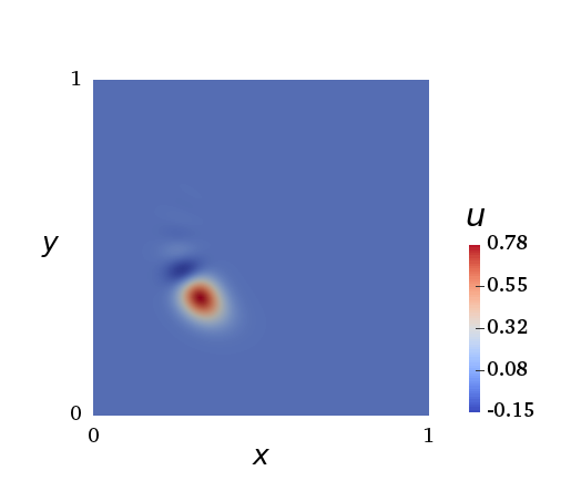
Space-time
  

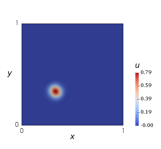
Figure 3: Comparison between sequential time stepping (top row) and space-time solution (bottom row) on mesh size $128^{3}$ (see Section 3.2.1). An initial pulse ($t=0$) is rotated under an advection field. The pulse at $t=1$ is plotted.

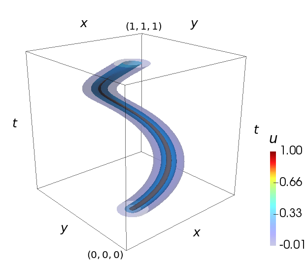
Figure 4: A contour plot of the rotating pulse in the space-time solution with $128^{3}$ grid (see Section 3.2.1). The rotating pulse renders a helical shape in the space-time domain

3.2 Uniform space-time mesh solutions and comparison to time-marching solutions

3.2.1 Advection-diffusion with smooth initial condition

We consider the two-dimensional, linear advection-diffusion equation (37) where the advection field ${\underline{a}}$ is purely rotational with unit angular velocity (see Figure 2, 2) and is given by

$${\underline{a}}({\underline{x}})=(-2\pi r_{y},2\pi r_{x}),$$ (38)

where $r_{x}$ and $r_{y}$ denote the distance of any point in the spatial domain from the center of the spatial domain $(\frac{1}{2},\frac{1}{2})$, i.e., $r_{x}=(x_{1}-0.5),r_{y}=(x_{2}-0.5)$. The speed of rotation is chosen in such a way that the pulse completes a full revolution at $t=1$.

The initial condition $u_{0}:U\rightarrow\mathbb{R}$ is a smooth function and is given by

$$u_{0}({\underline{x}})=e^{-\frac{(x-a)^{2}+(y-b)^{2}}{d^{2}}}.$$ (39)

This is essentially a Gaussian pulse with its center at $(a,b)=\left(\frac{1}{3},\frac{1}{3}\right)$ and thickness at base $\approx 2d=0.01$. The force $f$ on the right hand side is zero. The diffusivity value $\kappa$ is fixed at $10^{-4}$. The initial pulse keeps rotating in the domain as time evolves. Since the advection field has unit angular velocity, thus theoretically the center of the pulse at $t=0$ and $t=1$ should coincide. Since the field is also diffusive, the height of the pulse reduces with time.

Figure 4 shows contours of the solution $u$ in space-time. For clarity, only some of the iso-surfaces close to the pulse are shown. The rotation of the pulse is evident from a helical structure of the figure. The total number of elements in this case is $128\times 128\times 128$ with each element being a trilinear Lagrange element.

To see how the space-time solution behaves in comparison to the time-marching methods, we choose the Crank-Nicolson scheme to solve the same problem. This is reasonable since Crank-Nicolson is the simplest second order implicit time-marching method. To compare the methods, we discretize $\Omega=(0,1)^{2}\times(0,1]$ with the same number of elements in each dimension. As an example, Figure 3 compares the solution contours obtained by the sequential method on a 2D $(128\times 128)$ mesh marching over $128$ time steps against a space-time solution in 3D using a $128^{3}$ mesh. The right column of plots in this figure shows a cross-section of the pulses at both $t=0$ and $t=1$ along the plane ‘AB’, which passes through the center of initial pulse and is tangential to the local velocity vector (see Figure 2).

The Crank-Nicolson method is dispersive in nature and the solution exhibits a phase error; therefore the centers of the pulses between the two methods do not match. On the other hand, the space-time solution shows little dispersion and thus the peak centers align exactly. In regard to the undershoot around the pulse, the Crank-Nicolson solution shows a phase lag, whereas the space-time solution is visibly symmetric about the centre of the pulse. In both the solutions, however, the height of the peak at $t=1$ is roughly the same.

3.2.2 Pure advection with a discontinuous initial condition

Sequential (Crank-Nicolson)
$h=k=\frac{1}{64}$ $h=k=\frac{1}{128}$ $h=k=\frac{1}{256}$
   
Space-time
$h=\frac{1}{64}$ $h=\frac{1}{128}$ $h=\frac{1}{256}$
   

Figure 5: Sequential and space-time solutions for the case described in Section 3.2.2 on a uniform mesh of size $128^{3}$.

We solve (37) with the same advection field mentioned in (38) but this time with an initial condition that is not smooth in space. The initial data is given by,

$$u_{0}({\underline{x}})=\begin{cases}1&\text{if }(r_{1}^{2}+r_{2}^{2})\leq 1,\\ 0&\text{otherwise},\end{cases}$$ (40)

where ${\underline{r}}=({\underline{x}}-{\underline{x_{0}}})/\sigma$. Here ${\underline{x_{0}}}=\left(\frac{1}{3},\frac{1}{3}\right)$ is the initial position of the center of the circular pulse. The radius of this pulse is 1. Clearly, $u_{0}$ is discontinuous in space, (see Figure 2, 2). The diffusivity value $\kappa$ is set to $10^{-8}$ in this case. As earlier, the source term $f$ is zero. This choice of a negligible value of $\kappa$ effectively renders this case as a purely advective one. The global Peclet number is given as $Pe_{g}=\frac{|a|\cdot L}{\kappa}\approx 4.4\times 10^{8}$. As in the previous case, we discretize this problem through space-time as well as sequential time marching schemes and compare the pulse at $t=0$ and $t=1$. Figure 5 shows this comparison for both sequential and space-time method for three sizes of discretizations: $h=\frac{1}{64},\ \frac{1}{128}$ and $\frac{1}{256}$. The corresponding mesh-Peclet numbers are $Pe=\frac{|a|\cdot h}{2\kappa}\approx 3.47\times 10^{6},\ 1.74\times 10^{6}$ and $8.68\times 10^{5}$ respectively. As in the previous example, the plots are line cuts of the pulse onto the plane ‘AB’.

It can be noticed rightaway that both sequential and space-time formulation have difficulty approximating the discontinuous pulse, which can be attributed to the use of continuous Galerkin approximation when attempting to model a solution that is discontinuous. The final time representation of the pulse gets smoothened out in both cases, albeit to a different degree. But once again, the Crank-Nicolson method exhibits higher dispersion and phase errors, whereas the spacetime solution has zero phase error and a smaller dispersion. Once again, as in the previous example, the undershoot in the Crank-Nicolson method only takes place in the upwind direction whereas there is typically no undershoot in the downwind direction. But the spacetime solution does not display any directional preference for the undershoot.

3.3 Adaptive solutions

The examples considered in the previous section have solutions that show a high degree of spatial as well as temporal localization. That is, at a given instance of time, the solution function has a significant change in value only at some small area of the whole domain and zero at all other points of the domain. Moreover, as time evolves, there is a limited region where the solution changes. A significant portion of the domain never experiences any change in the solution with the evolution of time. This can be observed in Figure 4, where the solution is zero in all of the white region. This kind of problems are therefore perfect candidates where space-time adaptive refinement strategy can be useful. To show the effectiveness of adaptive refinement in a space-time simulation, we consider the following three examples.

3.3.1 The heat equation: estimator behavior in adaptive refinement

(a) Convergence of $\|e\|_{L^{2}(\Omega)}$

(b) Convergence of $\|\eta\|_{L^{2}(\Omega)}$

Figure 6: Comparison of the error indicator and the error in $L^{2}$-norm in both uniform and adaptive refinement

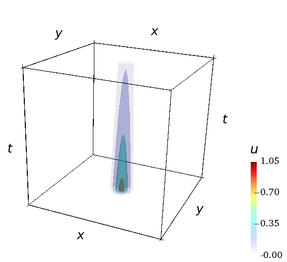
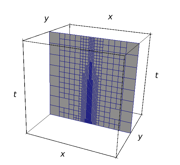
Figure 7: (Left) contours of the solution to the Gaussian heat source problem (35), (right) a $y-t$ slice at the final state of the adaptively refined mesh

We begin with a simple heat diffusion problem to illustrate adaptive refinement in space-time. We go back to the heat (35) with a forcing $f$ given by

$$f=-\left[2+\kappa\left(\frac{r_{x}^{2}+r_{y}^{2}}{d^{4}}\right)\left\{6+\frac{4}{d^{4}}(r_{x}^{4}-r_{x}^{2}r_{y}^{2}+r_{y}^{4})\right\}\right]e^{-2t-\frac{r_{x}^{2}+r_{y}^{2}}{d^{2}}}.$$ (41)

The analytical solution is given by

$$u=e^{-2t-\frac{r_{x}^{2}+r_{y}^{2}}{d^{2}}}.$$ (42)

This problem describes a Gaussian pulse at the center of the spatial domain $U$ diffusing as time evolves. In both (41) and (42), $r_{x}=x-x_{0}$ and $r_{y}=y-y_{0}$, where $(x_{0},y_{0})=(\frac{1}{2},\frac{1}{2})$ is the center of the heat pulse, $d=0.05$ is the “thickness” of the pulse. The diffusivity $\kappa=0.01$

To solve this problem adaptively, we begin with a very coarse 3D octree mesh (representing 2D in space and 1D in time). After computing the FEM space-time solution on this coarse mesh, we use the a posteriori error estimate presented in Theorem 2.7 to calculate the error indicator $\eta_{K}$ in each element ($K$ $\in$ $\mathcal{K}_{h}$). The elements, where the indicator $\eta_{K}$ is larger than a predetermined error tolerance, are refined. The refined mesh is then used to solve the same problem once again. This process is repeated for a few times till the error value in all the elements are smaller then the tolerance. Figure 6 shows comparisons of $\|u-u^{h}\|_{L^{2}(\Omega)}$ and $\|\eta\|_{L^{2}(\Omega)}$ for both uniform refinement and adaptive refinement. As expected, the error decreases much more rapidly when adaptive refinement is used.

A slice of the space-time mesh at the final refined state is shown in Figure 7. The slice is a $y$-constant plane, therefore the levels of refinement in the time direction are visible in this image. The largest element size in this slice is $h_{max}=\frac{1}{2^{3}}=\frac{1}{8}$ whereas the smallest element size is $h_{min}=\frac{1}{2^{7}}=\frac{1}{128}$. The ratio of $h_{max}$ to $h_{min}$ is thus $16$.

3.3.2 Advection-diffusion with smooth initial condition

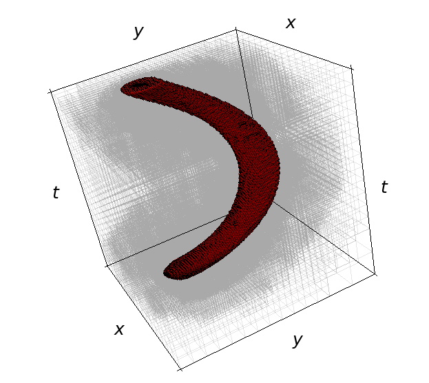
Figure 8: Space-time mesh at the final refinement state for the advection diffusion equation with a smooth bicosine pulse as the initial condition.

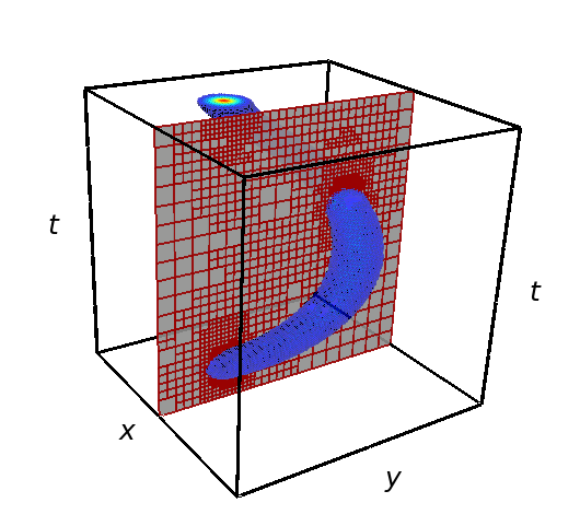
Figure 9: Space-time solution contour of a bi-cosine cone in a rotating field

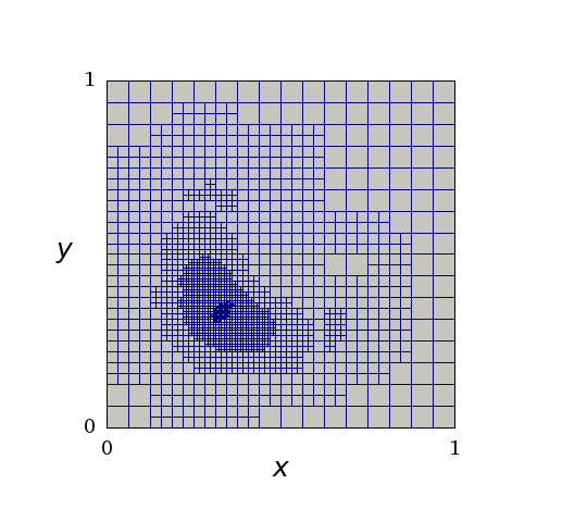
(a) An $x-y$ cross-section of the mesh $t=1$

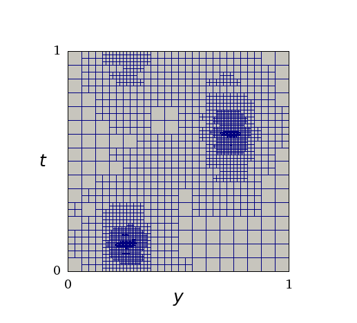
(b) A $y-t$ cross-section of the mesh at $x=0.5$

Figure 10: Slices of the final refined mesh for the adaptive solution of Section 3.3.2

$\kappa=10^{-2}$

$\kappa=10^{-4}$

$\kappa=10^{-6}$

$\kappa=10^{-8}$

Figure 11: Comparison of the cross-section of the pulse at $t=0$ and $t=1$ between a uniform mesh of $128^{3}$ and an adaptively refined mesh for different values of $\kappa$

Figure 9 shows the pulse contour for the advection diffusion problem (solved earlier using a uniform space-time mesh) with a smooth initial condition, along with the adaptively refined space-time mesh. A 2D slice of the same mesh is shown in Figure 9. Figure 10 shows the mesh slice at $t=1$. As expected, the refinement is clustered around the smooth pulse. Figure 10 on the other hand, shows a $y-t$ slice of the whole mesh. Once again, as seen from both these slices, the mesh size varies greatly between the finer and the coarser regions, which in this case, differs by a factor of $2^{5}$, i.e., the largest element has a size that is 32 times the size of the smallest element. Especially in relation to the mesh slice in Figure 10, it can be interpreted that different regions in the spatial domain are subjected to different “time steps” to reach the same final time. This is a very different behavior compared to a sequential solution where every region in the spatial domain has to go through the same number of time steps to reach the final time. Moreover, in sequential methods, the size of this time-step is often constrained by the minimum size of the mesh. For example, in this problem, the error in the solution is higher near the peak of the pulse and is gradually less as distance from the peak increases in space-time. This indicates that to achieve a reasonable accuracy, the regions near the pulse need to be resolved at least by elements of size $\approx\frac{1}{2^{8}}$ in space. This then implies that when using implicit time-marching methods such as the Crank-Nicolson method, the time-step size also needs to be $\mathcal{O}(h)$.

Figure 11 plots the cross-section of the pulse at $t=0$ and $t=1$ solved through both uniform-refinement and adaptive-refinement for four different values of $\kappa$. For all of these four cases, the uniformly refined mesh is of size $128^{3}$, i.e., $\textsc{DOF}=2146689$. The DOF in the adaptive meshes vary from case to case. As an example, for the case of $\kappa=10^{-8}$, the final refined state has $\textsc{DOF}=192507$.

Note that there is an appreciable decrease in the height of the pulse when $\kappa=10^{-4}$, but there is no such apparent loss when $\kappa=10^{-6}$ or $\kappa=10^{-8}$ which is correctly captured by the adaptive solutions. But the uniform $128^{3}$ mesh is unable to capture this; indicating that a further finer mesh is required. This shows that when $\kappa$ is very low, it is very difficult to resolve the peak without resorting to extremely small mesh sizes. A final observation is that $\kappa<10^{-6}$ can be used to model a “pure advection” case when considering $t\in[0,1]$ for this problem. Thus, this value of $\kappa$ is used to model a “purely advective” transport problem in the next example.

3.3.3 The advection-diffusion with sharp initial condition

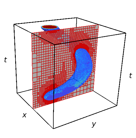
Figure 12: Contour of the discontinuous pulse through the space-time mesh

Figure 13: Cross section of the discontinuous pulse at $t=0$ and $t=1$

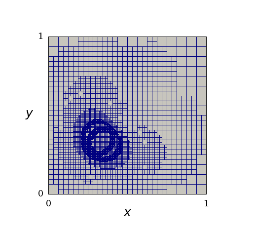
(a) An $x-y$ cross-section of the mesh $t=1$

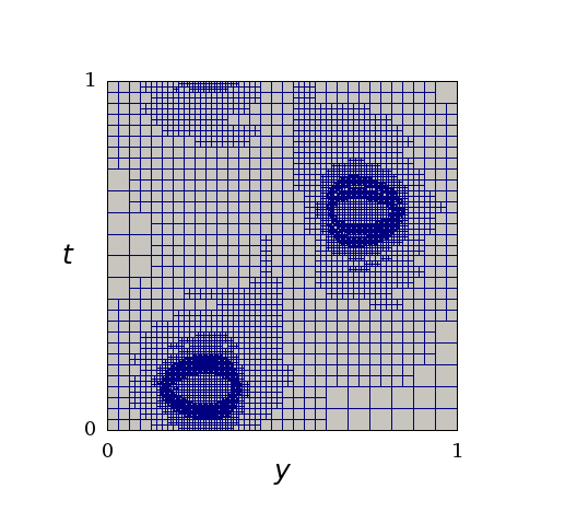
(b) A $y-t$ cross-section of the mesh at $x=0.5$

Figure 14: Slices of the final refined mesh for the adaptive solution of Section 3.3.3

Finally we take a quick glance at the adaptive solution of the pure advection problem with a discontinuous initial data. This is the same problem discussed in Section 3.2.2. Figure 13 shows contour of the discontinuous pulse in the space-time mesh at the final refinement state. Figure 13 shows the cross-section of the pulse at $t=0$ and at $t=1$. The interior of the pulse has bigger elements than the boundary of the pulse where the discontinuity lies. As mentioned before, the solution quality near the discontinuity is restricted by the underlying continuous Galerkin method which is not ideal at approximating discontinuities. This produces overshoot and undershoot near the discontinuity which results in higher residual and eventually high refinement near the discontinuity. Figure 14 shows a 2D $x-y$ slice and Figure 14 shows a 2D $y-t$ slice of the final refined mesh. Once again the mesh size varies greatly throughout the domain.

4 Conclusions

In this work we considered a coupled-space-time finite element formulation of the time-dependent advection-diffusion equation using continuous Galerkin method. Such an operator can be cast as a generalized advection-diffusion equation in the space-time domain. Due to the non-dissipative nature of the advection operator, the discrete problem corresponding to these equations may become unstable. To overcome this lack of stability of the discrete variational problem, we formulate an analogue of the Galerkin/least square (GLS) stabilization method in space-time. We show that the GLS-type regularization results in a stable discrete variational problem. We subsequently prove a priori error estimates; and also present a residual based a posteriori error estimate that is used to achieve adaptive refinement in space-time.

We test our method on various numerical examples such as the heat equation (smooth solution) and the advection-diffusion equation (both smooth and non-smooth solution). An interesting feature of the space-time solution is that the solution does not suffer any phase error. Also when approximating a discontinuous solution, the space-time method display considerably less oscillations compared to a sequential method of similar accuracy (Crank-Nicolson method). When coupled with an adaptive mesh refinement strategy, both smooth and discontinuous fields can be approximated closely and can even model no-loss solution in the presence of negligible diffusion.

Potential future work include extension to other stabilization techniques such the streamline upwind Petrov Galerkin method and the variational multiscale method. In addition, nonlinear equations pose significantly different challenges compared to linear PDEs, therefore nonlinear operators such as the Cahn-Hilliard system or the Navier-Stokes equation need to be considered and analyzed with such a formulation. Furthermore, all the examples in this paper were obtained using 3D space-time (i.e., 2D + time) meshes, thus another avenue of future works include extension of the computational meshes to four-dimensions.

5 Acknowledgements

This work was partly supported by the National Science Foundation under the grants NSF LEAP-HI 2053760, NSF 1935255.

Appendix A Proofs for Section 2

A.1 Lemma 2.1 (Boundedness)

Proof of Lemma 2.1.

We consider each of the inner product in (23) and bound them from above.

1. The first term $(v^{h}_{t},w^{h})$ is first integration by parts and then each of the resulting term is estimated from below:

   $$|(v^{h}_{t},w^{h})| =\left|\int_{0}^{T}\int_{U}v^{h}_{t}w^{h}dUdt\right|=\left|-\int_{0}^{T}\int_{U}v^{h}w^{h}_{t}dUdt+\int_{\Gamma_{{}_{T}}}v^{h}w^{h}dS\right|$$

   $$\leq\left|-\int_{0}^{T}\int_{U}v^{h}w^{h}_{t}dUdt\right|+\left|\int_{\Gamma_{{}_{T}}}v^{h}w^{h}dS\right|$$

   $$\leq\|v^{h}\|_{L^{2}(\Omega)}\|w^{h}_{t}\|_{L^{2}(\Omega)}+\|v^{h}\|_{L^{2}(\Gamma_{{}_{T}})}\|w^{h}\|_{L^{2}(\Gamma_{{}_{T}})}$$

2. Each of the next six terms in (23) can be easily bounded from above by applying Cauchy-Schwarz inequality

   $$|({\underline{a}}\cdot\underline{{\nabla}\mkern-4.0mu}\mkern 4.0muv^{h},w^{h})|\leq\|{\underline{a}}\cdot\underline{{\nabla}\mkern-4.0mu}\mkern 4.0muv^{h}\|_{L^{2}(\Omega)}\|w^{h}\|_{L^{2}(\Omega)}\leq|{\underline{a}}|\|\underline{{\nabla}\mkern-4.0mu}\mkern 4.0muv^{h}\|_{L^{2}(\Omega)}\|w^{h}\|_{L^{2}(\Omega)}$$

3. $$|(\kappa\underline{{\nabla}\mkern-4.0mu}\mkern 4.0muv^{h},\underline{{\nabla}\mkern-4.0mu}\mkern 4.0muw^{h})|\leq\kappa\|\underline{{\nabla}\mkern-4.0mu}\mkern 4.0muv^{h}\|_{L^{2}(\Omega)}\|\underline{{\nabla}\mkern-4.0mu}\mkern 4.0muw^{h}\|_{L^{2}(\Omega)}$$

4. $$|\epsilon(v^{h}_{t},w^{h}_{t})|\leq\epsilon\|v^{h}_{t}\|_{L^{2}(\Omega)}\|w^{h}_{t}\|_{L^{2}(\Omega)}$$

5. $$|\epsilon({\underline{a}}\cdot\underline{{\nabla}\mkern-4.0mu}\mkern 4.0muv^{h},{\underline{a}}\cdot\underline{{\nabla}\mkern-4.0mu}\mkern 4.0muw^{h})|\leq\epsilon\left(\|{\underline{a}}\|_{L^{\infty}(\Omega)}\|\underline{{\nabla}\mkern-4.0mu}\mkern 4.0muv^{h}\|_{L^{2}(\Omega)}\right)\left(\|{\underline{a}}\|_{L^{\infty}(\Omega)}\|\underline{{\nabla}\mkern-4.0mu}\mkern 4.0muw^{h}\|_{L^{2}(\Omega)}\right)$$

6. $$|\epsilon(v^{h}_{t},{\underline{a}}\cdot\underline{{\nabla}\mkern-4.0mu}\mkern 4.0muw^{h})|\leq\epsilon\|v^{h}_{t}\|_{L^{2}(\Omega)}\|{\underline{a}}\|_{L^{\infty}(\Omega)}\|\underline{{\nabla}\mkern-4.0mu}\mkern 4.0muw^{h}\|_{L^{2}(\Omega)}$$

7. $$|\epsilon({\underline{a}}\cdot\underline{{\nabla}\mkern-4.0mu}\mkern 4.0muv^{h},w^{h}_{t})|\leq\epsilon\|{\underline{a}}\|_{L^{\infty}(\Omega)}\|\underline{{\nabla}\mkern-4.0mu}\mkern 4.0muv^{h}\|_{L^{2}(\Omega)}\|w^{h}_{t}\|_{L^{2}(\Omega)}$$

8. While trying to put an upper bound to $\epsilon\kappa(\underline{{\nabla}\mkern-4.0mu}\mkern 4.0muv^{h}_{t},\underline{{\nabla}\mkern-4.0mu}\mkern 4.0muw^{h})$, we note that $\underline{{\nabla}\mkern-4.0mu}\mkern 4.0muv^{h}_{t}$ is a second derivative on $v^{h}$ with respect to both space and time. We estimate this term by only the spatial derivatives through the use of the inverse estimates.

   $$\|\underline{{\nabla}\mkern-4.0mu}\mkern 4.0muv^{h}_{t}\|_{L^{2}(\Omega)}=\int_{\Omega}\left[|\underline{{\nabla}\mkern-4.0mu}\mkern 4.0muv^{h}_{t}|^{2}\right]d\Omega=\int_{\Omega}\left[\sum_{i=1}^{n}|v^{h}_{tx_{i}}|^{2}\right]d\Omega=\sum_{i=1}^{n}\left[\int_{\Omega}|v^{h}_{tx_{i}}|^{2}d\Omega\right]$$

   The integratioin over $\Omega$ is equal to the sum of integration over all the individual elements in the mesh, i.e.,

   $$\sum_{i=1}^{n}\left[\int_{\Omega}|v^{h}_{tx_{i}}|^{2}d\Omega\right]=\sum_{i=1}^{n}\sum_{K\in\mathcal{K}_{h}}\left[\int_{K}|v^{h}_{tx_{i}}|^{2}dK\right]=\sum_{i=1}^{n}\sum_{K\in\mathcal{K}_{h}}\|v^{h}_{tx_{i}}\|_{L^{2}(K)}^{2}$$

   There exist a positive constant $C_{I,1}$ such that

   $$\|v^{h}_{tx_{i}}\|_{L^{2}(K)}^{2}\leq C_{I,1}^{2}h^{-2}\|v^{h}_{x_{i}}\|_{L^{2}(K)}^{2}\textrm{ for }i=1,2,...,n$$

   Therefore we have,

   $$\|\underline{{\nabla}\mkern-4.0mu}\mkern 4.0muv^{h}_{t}\|_{L^{2}(\Omega)} \leq\sum_{i=1}^{n}\sum_{K\in\mathcal{K}_{h}}C_{I,1}^{2}h^{-2}\|v^{h}_{x_{i}}\|_{L^{2}(K)}^{2}=C_{I,1}h^{-2}\sum_{i=1}^{n}\sum_{K\in\mathcal{K}_{h}}\left[\int_{K}|v^{h}_{x_{i}}|^{2}dK\right]$$

   $$=C_{I,1}^{2}h^{-2}\sum_{i=1}^{n}\left[\int_{\Omega}|v^{h}_{x_{i}}|^{2}d\Omega\right]=C_{I,1}^{2}h^{-2}\int_{\Omega}\left[\sum_{i=1}^{n}|v^{h}_{x_{i}}|^{2}\right]d\Omega=C_{I,1}^{2}h^{-2}\|\underline{{\nabla}\mkern-4.0mu}\mkern 4.0muv^{h}\|_{L^{2}(\Omega)}$$

   So finally applying Cauchy Schwarz inequality on $\epsilon\kappa(\underline{{\nabla}\mkern-4.0mu}\mkern 4.0muv^{h}_{t},\underline{{\nabla}\mkern-4.0mu}\mkern 4.0muw^{h})$, we have,

   $$|\epsilon\kappa(\underline{{\nabla}\mkern-4.0mu}\mkern 4.0muv^{h}_{t},\underline{{\nabla}\mkern-4.0mu}\mkern 4.0muw^{h})| \leq\epsilon\kappa\|\underline{{\nabla}\mkern-4.0mu}\mkern 4.0muv^{h}_{t}\|_{L^{2}(\Omega)}\|\underline{{\nabla}\mkern-4.0mu}\mkern 4.0muw^{h}\|_{L^{2}(\Omega)}\leq\epsilon\kappa C_{I,1}h^{-1}\|\underline{{\nabla}\mkern-4.0mu}\mkern 4.0muv^{h}\|_{L^{2}(\Omega)}\|\underline{{\nabla}\mkern-4.0mu}\mkern 4.0muw^{h}\|_{L^{2}(\Omega)}$$

9. The next term $\epsilon\kappa(\underline{{\nabla}\mkern-4.0mu}\mkern 4.0muv^{h},\underline{{\nabla}\mkern-4.0mu}\mkern 4.0muw^{h}_{t})$ similar to the previous one and can be estimated in the same way

   $$|\epsilon\kappa(\underline{{\nabla}\mkern-4.0mu}\mkern 4.0muv^{h},\underline{{\nabla}\mkern-4.0mu}\mkern 4.0muw^{h}_{t})|\leq\epsilon\kappa\|\underline{{\nabla}\mkern-4.0mu}\mkern 4.0muw^{h}\|_{L^{2}(\Omega)}\|\underline{{\nabla}\mkern-4.0mu}\mkern 4.0muw^{h}_{t}\|_{L^{2}(\Omega)}\leq\epsilon\kappa C_{I,1}h^{-1}\|\underline{{\nabla}\mkern-4.0mu}\mkern 4.0muv^{h}\|_{L^{2}(\Omega)}\|\underline{{\nabla}\mkern-4.0mu}\mkern 4.0muw^{h}\|_{L^{2}(\Omega)}$$

Now we combine all these terms using Cauchy’s inequality and get,

$$|b^{h}(v^{h},w^{h})|\leq\left[X(v^{h})\right]^{\frac{1}{2}}\left[Y(w^{h})\right]^{\frac{1}{2}}$$ (43)

where, $X(v^{h})$ and $Y(w^{h})$ are as follows,

$$X(v^{h}) =\left[\epsilon^{-1}\|v^{h}\|_{L^{2}(\Omega)}^{2}+\|v^{h}\|_{L^{2}(\Gamma_{{}_{T}})}^{2}+2\epsilon\|v^{h}_{t}\|_{L^{2}(\Omega)}^{2}+\left((1+2\epsilon)\|{\underline{a}}\|_{L^{\infty}(\Omega)}^{2}+\left(\frac{\epsilon}{h}\right)^{2}C_{I,1}^{2}+2\kappa\right)\|\underline{{\nabla}\mkern-4.0mu}\mkern 4.0muv^{h}\|_{L^{2}(\Omega)}^{2}\right]^{\frac{1}{2}}$$

$$Y(w^{h}) =\left[\|w^{h}\|_{L^{2}(\Gamma_{{}_{T}})}^{2}+(1+3\epsilon)\|w^{h}_{t}\|_{L^{2}(\Omega)}^{2}+\left(2\epsilon\|{\underline{a}}\|_{L^{\infty}(\Omega)}^{2}+\left(\frac{\epsilon}{h}\right)^{2}C_{I,1}^{2}+2(\kappa+\epsilon)\right)\|\underline{{\nabla}\mkern-4.0mu}\mkern 4.0muw^{h}\|_{L^{2}(\Omega)}^{2}\right]^{\frac{1}{2}}$$

The inequality 43 can then be estimated as

$$|b^{h}(v^{h},w^{h})|\leq\mu_{b}\|v^{h}\|_{V_{h},*}\|w^{h}\|_{V_{h}}$$ (44)

∎

A.2 Lemma 2.2 (Coercivity)

Proof of Lemma 2.2.

From (23) we have,

$$\begin{split}b^{h}(v^{h},v^{h})&=\int_{0}^{T}\int_{U}\Big{[}v^{h}v^{h}_{t}+v^{h}({\underline{a}}\cdot\underline{{\nabla}\mkern-4.0mu}\mkern 4.0muv^{h})+\kappa|\underline{{\nabla}\mkern-4.0mu}\mkern 4.0muv^{h}|^{2}+\epsilon(v^{h}_{t})^{2}+2\epsilon v^{h}_{t}({\underline{a}}\cdot\underline{{\nabla}\mkern-4.0mu}\mkern 4.0muv^{h})\\ &\quad+2\epsilon\kappa(\underline{{\nabla}\mkern-4.0mu}\mkern 4.0muv^{h}\cdot\underline{{\nabla}\mkern-4.0mu}\mkern 4.0muv^{h}_{t})+\epsilon({\underline{a}}\cdot\underline{{\nabla}\mkern-4.0mu}\mkern 4.0muv^{h})^{2}\Big{]}dUdt\\ &=\int_{0}^{T}\int_{U}\Big{[}v^{h}v^{h}_{t}+2\epsilon\kappa(\underline{{\nabla}\mkern-4.0mu}\mkern 4.0muv^{h}\cdot\underline{{\nabla}\mkern-4.0mu}\mkern 4.0muv^{h}_{t})+v^{h}({\underline{a}}\cdot\underline{{\nabla}\mkern-4.0mu}\mkern 4.0muv^{h})+\kappa|\underline{{\nabla}\mkern-4.0mu}\mkern 4.0muv^{h}|^{2}+\epsilon(v^{h}_{t})^{2}\\ &\quad+2\epsilon v^{h}_{t}({\underline{a}}\cdot\underline{{\nabla}\mkern-4.0mu}\mkern 4.0muv^{h})+\epsilon({\underline{a}}\cdot\underline{{\nabla}\mkern-4.0mu}\mkern 4.0muv^{h})^{2}\Big{]}dUdt.\end{split}$$

The first two terms in the above expression are related to the trace of the function $v^{h}$ restricted to the final time boundary:

$$\int_{0}^{T}\int_{U}v^{h}v^{h}_{t}+2\epsilon\kappa(\underline{{\nabla}\mkern-4.0mu}\mkern 4.0muv^{h}\cdot\underline{{\nabla}\mkern-4.0mu}\mkern 4.0muv^{h}_{t})dUdt =\int_{0}^{T}\int_{U}\left[\frac{\partial}{\partial t}\left(\frac{(v^{h})^{2}}{2}\right)+\epsilon\kappa\frac{\partial}{\partial t}\left(\underline{{\nabla}\mkern-4.0mu}\mkern 4.0muv^{h}\cdot\underline{{\nabla}\mkern-4.0mu}\mkern 4.0muv^{h}\right)\right]dUdt$$

$$=\frac{1}{2}\left(\|v^{h}\|_{L^{2}(\Gamma_{{}_{T}})}^{2}-\|v^{h}\|_{L^{2}(\Gamma_{{}_{0}})}^{2}\right)+\epsilon\kappa(\|\underline{{\nabla}\mkern-4.0mu}\mkern 4.0muv^{h}\|_{L^{2}(\Gamma_{{}_{T}})}^{2}-\|\underline{{\nabla}\mkern-4.0mu}\mkern 4.0muv^{h}\|_{L^{2}(\Gamma_{{}_{0}})}^{2})$$

$$=\frac{1}{2}\|v^{h}\|_{L^{2}(\Gamma_{{}_{T}})}^{2}+\epsilon\kappa\|\underline{{\nabla}\mkern-4.0mu}\mkern 4.0muv^{h}\|_{L^{2}(\Gamma_{{}_{T}})}^{2}.$$

Because of the divergence-free velocity field, the third term evaluates to zero:

$$\int_{0}^{T}\int_{U}v^{h}({\underline{a}}\cdot\underline{{\nabla}\mkern-4.0mu}\mkern 4.0muv^{h})dUdt =\int_{0}^{T}\int_{U}{\underline{a}}\cdot(v^{h}\underline{{\nabla}\mkern-4.0mu}\mkern 4.0muv^{h})=\frac{1}{2}\int_{0}^{T}\int_{U}{\underline{a}}\cdot\underline{{\nabla}\mkern-4.0mu}\mkern 4.0mu(v^{h})^{2}=\frac{1}{2}\int_{0}^{T}\int_{U}\underline{{\nabla}\mkern-4.0mu}\mkern 4.0mu\cdot({\underline{a}}(v^{h})^{2})$$

$$=\frac{1}{2}\int_{0}^{T}\int_{\partial U}\hat{n}\cdot({\underline{a}}(v^{h})^{2})dSdt=0$$

since $v^{h}=0$ on $\partial U$. Finally, the last four terms can be taken collectively,

$$S =\int_{0}^{T}\int_{U}\left[\kappa|\underline{{\nabla}\mkern-4.0mu}\mkern 4.0muv^{h}|^{2}+\epsilon(v^{h}_{t})^{2}+2\epsilon v^{h}_{t}({\underline{a}}\cdot\underline{{\nabla}\mkern-4.0mu}\mkern 4.0muv^{h})+\epsilon({\underline{a}}\cdot\underline{{\nabla}\mkern-4.0mu}\mkern 4.0muv^{h})^{2}\right]dUdt$$

$$=\int_{0}^{T}\int_{U}\left[\kappa\sum_{i=1}^{n}(v^{h}_{x_{i}})^{2}+\epsilon(v^{h}_{t})^{2}+2\epsilon\sum_{i=1}^{n}v^{h}_{t}a_{i}v^{h}_{x_{i}}+\epsilon\left(\sum_{i=1}^{n}(a_{i}v^{h}_{x_{i}})^{2}+\sum_{\begin{subarray}{c}i,j=1\\ j\neq i\end{subarray}}^{n}a_{i}a_{j}v^{h}_{x_{i}}v^{h}_{x_{j}}\right)\right]dUdt$$

$$=\int_{0}^{T}\int_{U}\left[\sum_{i=1}^{n}(\kappa+\epsilon a_{i}^{2})(v^{h}_{x_{i}})^{2}+\epsilon(v^{h}_{t})^{2}+\sum_{i=1}^{n}2\epsilon a_{i}v^{h}_{t}v^{h}_{x_{i}}+\sum_{\begin{subarray}{c}i,j=1\\ j\neq i\end{subarray}}^{n}a_{i}a_{j}v^{h}_{x_{i}}v^{h}_{x_{j}}\right]dUdt$$

$$=\int_{0}^{T}\int_{U}\left(\underline{\widetilde{\nabla}\mkern-4.0mu}\mkern 4.0muv^{h}\cdot{\underline{\underline{M}}}\cdot\underline{\widetilde{\nabla}\mkern-4.0mu}\mkern 4.0muv^{h}\right)dUdt,$$

where $\underline{\widetilde{\nabla}\mkern-4.0mu}\mkern 4.0muv^{h}$ is defined in 4, and ${\underline{\underline{M}}}$ is defined as,

$${\underline{\underline{M}}}=\begin{bmatrix}\kappa+\epsilon a_{1}^{2}&\epsilon a_{1}a_{2}&\cdots&\epsilon a_{1}a_{n}&\epsilon a_{1}\\ \epsilon a_{1}a_{2}&\kappa+\epsilon a_{2}^{2}&\cdots&\epsilon a_{2}a_{n}&\epsilon a_{2}\\ \vdots&\vdots&\ddots&\vdots&\vdots\\ \epsilon a_{1}a_{n}&\epsilon a_{2}a_{n}&\cdots&\kappa+\epsilon a_{n}^{2}&\epsilon a_{n}\\ \epsilon a_{1}&\epsilon a_{2}&\cdots&\epsilon a_{n}&\epsilon\end{bmatrix}_{(n+1)\times(n+1)}.$$ (45)

The matrix ${\underline{\underline{M}}}$ plays a role that is similar to the ${\underline{\underline{A}}}$ matrix defined in equation  6. For $n=2$, the eigenvalues of ${\underline{\underline{M}}}$ are

$$\lambda_{1} =k,$$

$$\lambda_{2} =\frac{1}{2}\left[k+\epsilon(1+|{\underline{a}}|^{2})-\sqrt{[k+\epsilon(1+|{\underline{a}}|^{2})]^{2}-4\kappa\epsilon}\right],$$

$$\lambda_{3} =\frac{1}{2}\left[k+\epsilon(1+|{\underline{a}}|^{2})+\sqrt{[k+\epsilon(1+|{\underline{a}}|^{2})]^{2}-4\kappa\epsilon}\right].$$

The matrix ${\underline{\underline{M}}}$ is symmetric and positive definite, thus its minimum eigenvalue is greater than zero. Thus for any vector $y\in\mathbb{R}^{n+1}$, we have ${\underline{y}}^{T}{\underline{\underline{M}}}{\underline{y}}>\epsilon|y|^{2}>0$. Therefore,

$$S\geq\int_{0}^{T}\int_{U}\epsilon|{\underline{D}}v^{h}|^{2}dUdt=\epsilon\|\underline{\widetilde{\nabla}\mkern-4.0mu}\mkern 4.0muv^{h}\|_{L^{2}(\Omega)}^{2}.$$

Putting it all together,

$$b^{h}(v^{h},v^{h}) \geq\frac{1}{2}\|v^{h}\|_{L^{2}(\Gamma_{{}_{T}})}^{2}+\epsilon\kappa\|\underline{{\nabla}\mkern-4.0mu}\mkern 4.0muv^{h}\|_{L^{2}(\Gamma_{{}_{T}})}^{2}+\epsilon\|\underline{\widetilde{\nabla}\mkern-4.0mu}\mkern 4.0muv^{h}\|_{L^{2}(\Omega)}$$

$$\geq\frac{1}{2}\|v^{h}\|_{L^{2}(\Gamma_{{}_{T}})}^{2}+\epsilon\|\underline{\widetilde{\nabla}\mkern-4.0mu}\mkern 4.0muv^{h}\|_{L^{2}(\Omega)}$$

$$=\frac{1}{2}\|v^{h}\|_{L^{2}(\Gamma_{{}_{T}})}^{2}+\epsilon\left(\|\underline{{\nabla}\mkern-4.0mu}\mkern 4.0muv^{h}\|_{L^{2}(\Omega)}+\|v^{h}_{t}\|_{L^{2}(\Omega)}\right)$$

$$=\mu_{c}\|v^{h}\|_{V_{h}},$$

where $0\leq\mu_{c}\leq 1$. ∎

A.3 Proof of Lemma 2.2 when higher order basis functions are used

When higher order basis functions are used, the stability of the discrete problem (20) can be proved in a simpler way using a different norm. We have, from the left hand side of equation  (19),

$$b^{h}(v^{h},w^{h}) =(\mathscr{L}v^{h},w^{h})+\epsilon(\mathscr{L}v^{h},\mathscr{L}w^{h})$$ (46)

$$=(v^{h}_{t},w^{h})+({\underline{a}}\cdot\underline{{\nabla}\mkern-4.0mu}\mkern 4.0muv^{h},w^{h})+(\kappa\underline{{\nabla}\mkern-4.0mu}\mkern 4.0muv^{h},\underline{{\nabla}\mkern-4.0mu}\mkern 4.0muw^{h})$$ (47)

$$\qquad+\epsilon\big{(}[v^{h}_{t}+{\underline{a}}\cdot\underline{{\nabla}\mkern-4.0mu}\mkern 4.0muv^{h}-\kappa\Delta v^{h}],[w^{h}_{t}+{\underline{a}}\cdot\underline{{\nabla}\mkern-4.0mu}\mkern 4.0muw^{h}-\kappa\Delta w^{h}]\big{)}$$ (48)

Therefore,

$$b^{h}(v^{h},v^{h}) =(\mathscr{L}v^{h},v^{h})+\epsilon(\mathscr{L}v^{h},\mathscr{L}v^{h})$$

$$=(v^{h}_{t},v^{h})+({\underline{a}}\cdot\underline{{\nabla}\mkern-4.0mu}\mkern 4.0muv^{h},v^{h})+(\kappa\underline{{\nabla}\mkern-4.0mu}\mkern 4.0muv^{h},\underline{{\nabla}\mkern-4.0mu}\mkern 4.0muv^{h})$$

$$\qquad+\epsilon\big{(}[v^{h}_{t}+{\underline{a}}\cdot\underline{{\nabla}\mkern-4.0mu}\mkern 4.0muv^{h}-\kappa\Delta v^{h}],[v^{h}_{t}+{\underline{a}}\cdot\underline{{\nabla}\mkern-4.0mu}\mkern 4.0muv^{h}-\kappa\Delta v^{h}]\big{)}$$

$$=\int_{0}^{T}\int_{U}\Big{[}v^{h}v^{h}_{t}+v^{h}({\underline{a}}\cdot\underline{{\nabla}\mkern-4.0mu}\mkern 4.0muv^{h})+\kappa(\underline{{\nabla}\mkern-4.0mu}\mkern 4.0muv^{h}\cdot\underline{{\nabla}\mkern-4.0mu}\mkern 4.0muv^{h})$$

$$\qquad\qquad\qquad\qquad\qquad+\epsilon(v^{h}_{t}+{\underline{a}}\cdot\underline{{\nabla}\mkern-4.0mu}\mkern 4.0muv^{h}-\kappa\Delta v^{h})^{2}\Big{]}dUdt$$

$$=\int_{0}^{T}\int_{U}\frac{\partial}{\partial t}\left(\frac{(v^{h})^{2}}{2}\right)dUdt+\int_{0}^{T}\int_{U}\underline{{\nabla}\mkern-4.0mu}\mkern 4.0mu\cdot\left(\frac{{\underline{a}}(v^{h})^{2}}{2}\right)dUdt+\int_{0}^{T}\int_{U}\kappa|\underline{{\nabla}\mkern-4.0mu}\mkern 4.0muv^{h}|^{2}dUdt$$

$$\quad+\int_{0}^{T}\int_{U}\epsilon(v^{h}_{t}+{\underline{a}}\cdot\underline{{\nabla}\mkern-4.0mu}\mkern 4.0muv^{h}-\kappa\Delta v^{h})^{2}dUdt$$

$$=\frac{1}{2}\left(\|v^{h}\|_{L^{2}(\Gamma_{{}_{T}})}^{2}-\|v^{h}\|_{L^{2}(\Gamma_{{}_{0}})}^{2}\right)+\frac{1}{2}\int_{0}^{T}\int_{\partial U}\hat{n}\cdot({\underline{a}}(v^{h})^{2})dSdt+\kappa\|\underline{{\nabla}\mkern-4.0mu}\mkern 4.0muv^{h}\|_{L^{2}(\Omega)}^{2}$$

$$\qquad+\int_{0}^{T}\int_{U}\epsilon\{(v^{h}_{t}+{\underline{a}}\cdot\underline{{\nabla}\mkern-4.0mu}\mkern 4.0muv^{h})-\kappa\Delta v^{h}\}^{2}dUdt$$

$$=\left(\frac{1}{2}\|v^{h}\|_{L^{2}(\Gamma_{{}_{T}})}^{2}-0\right)+0+\kappa\|\underline{{\nabla}\mkern-4.0mu}\mkern 4.0muv^{h}\|_{L^{2}(\Omega)}^{2}$$

$$\qquad+\int_{0}^{T}\int_{U}\epsilon\left[(v^{h}_{t}+{\underline{a}}\cdot\underline{{\nabla}\mkern-4.0mu}\mkern 4.0muv^{h})^{2}+(\kappa\Delta v^{h})^{2}-2(v^{h}_{t}+{\underline{a}}\cdot\underline{{\nabla}\mkern-4.0mu}\mkern 4.0muv^{h})(\kappa\Delta v^{h})\right]dUdt$$

$$=\frac{1}{2}\|v^{h}\|_{L^{2}(\Gamma_{{}_{T}})}^{2}+\kappa\|\underline{{\nabla}\mkern-4.0mu}\mkern 4.0muv^{h}\|_{L^{2}(\Omega)}^{2}+\|\epsilon(v^{h}_{t}+{\underline{a}}\cdot\underline{{\nabla}\mkern-4.0mu}\mkern 4.0muv^{h})\|_{L^{2}(\Omega)}^{2}+\epsilon\kappa^{2}\|\Delta v^{h}\|_{L^{2}(\Omega)}$$

$$\qquad-\int_{0}^{T}\int_{U}\epsilon\kappa\left[2v^{h}_{t}\Delta v^{h}\right]dUdt-\int_{0}^{T}\int_{U}\epsilon\kappa\left[2({\underline{a}}\cdot\underline{{\nabla}\mkern-4.0mu}\mkern 4.0muv^{h})(\Delta v^{h})\right]dUdt$$

The last two integrals can now be examined separately. The first one of them can be evaluated as

$$-\int_{0}^{T}\int_{U}\epsilon\kappa\left[2v^{h}_{t}\Delta v^{h}\right]dUdt =\int_{0}^{T}\int_{U}\epsilon\kappa(2\underline{{\nabla}\mkern-4.0mu}\mkern 4.0muv^{h}_{t}\cdot\underline{{\nabla}\mkern-4.0mu}\mkern 4.0muv^{h})dUdt=\int_{0}^{T}\int_{U}\epsilon\kappa\frac{\partial}{\partial t}|\underline{{\nabla}\mkern-4.0mu}\mkern 4.0muv^{h}|^{2}dUdt$$

$$=\epsilon\kappa(\|\underline{{\nabla}\mkern-4.0mu}\mkern 4.0muv^{h}\|_{L^{2}(\Gamma_{{}_{T}})}^{2}-\|\underline{{\nabla}\mkern-4.0mu}\mkern 4.0muv^{h}\|_{L^{2}(\Gamma_{{}_{0}})}^{2})=\epsilon\kappa\|\underline{{\nabla}\mkern-4.0mu}\mkern 4.0muv^{h}\|_{L^{2}(\Gamma_{{}_{T}})}^{2}$$

And the very last integral can be estimated with the help of inverse estimates,

$$-\int_{0}^{T}\int_{U}\epsilon\kappa\left[2({\underline{a}}\cdot\underline{{\nabla}\mkern-4.0mu}\mkern 4.0muv^{h})(\Delta v^{h})\right]dUdt =-2\epsilon\kappa({\underline{a}}\cdot\underline{{\nabla}\mkern-4.0mu}\mkern 4.0muv^{h},\Delta v^{h})$$

$$\geq-2\epsilon\kappa|({\underline{a}}\cdot\underline{{\nabla}\mkern-4.0mu}\mkern 4.0muv^{h},\Delta v^{h})|$$

$$\geq-2\epsilon\kappa\|{\underline{a}}\|_{L^{\infty}(\Omega)}\|\underline{{\nabla}\mkern-4.0mu}\mkern 4.0muv^{h}\|_{L^{2}(\Omega)}Ch^{-1}\|\underline{{\nabla}\mkern-4.0mu}\mkern 4.0muv^{h}\|_{L^{2}(\Omega)}$$

$$=-2Ch^{-1}\epsilon\kappa\|{\underline{a}}\|_{L^{\infty}(\Omega)}\|\underline{{\nabla}\mkern-4.0mu}\mkern 4.0muv^{h}\|_{L^{2}(\Omega)}$$

Therefore

$$b^{h}(v^{h},v^{h}) \geq\frac{1}{2}\|v^{h}\|_{L^{2}(\Gamma_{{}_{T}})}^{2}+\kappa\|\underline{{\nabla}\mkern-4.0mu}\mkern 4.0muv^{h}\|_{L^{2}(\Omega)}^{2}+\|\epsilon(v^{h}_{t}+{\underline{a}}\cdot\underline{{\nabla}\mkern-4.0mu}\mkern 4.0muv^{h})\|_{L^{2}(\Omega)}^{2}+\epsilon\kappa^{2}\|\Delta v^{h}\|_{L^{2}(\Omega)}$$ (49)

$$\qquad+\epsilon\kappa\|\underline{{\nabla}\mkern-4.0mu}\mkern 4.0muv^{h}\|_{L^{2}(\Gamma_{{}_{T}})}^{2}-2Ch^{-1}\epsilon\kappa\|{\underline{a}}\|_{L^{\infty}(\Omega)}\|\underline{{\nabla}\mkern-4.0mu}\mkern 4.0muv^{h}\|_{L^{2}(\Omega)}$$ (50)

$$=\frac{1}{2}\|v^{h}\|_{L^{2}(\Gamma_{{}_{T}})}^{2}+\epsilon\kappa\|\underline{{\nabla}\mkern-4.0mu}\mkern 4.0muv^{h}\|_{L^{2}(\Gamma_{{}_{T}})}^{2}+\|\epsilon(v^{h}_{t}+{\underline{a}}\cdot\underline{{\nabla}\mkern-4.0mu}\mkern 4.0muv^{h})\|_{L^{2}(\Omega)}^{2}$$ (51)

$$\qquad+(\kappa-2Ch^{-1}\epsilon\kappa\|{\underline{a}}\|_{L^{\infty}(\Omega)})\|\underline{{\nabla}\mkern-4.0mu}\mkern 4.0muv^{h}\|_{L^{2}(\Omega)}+\epsilon\kappa^{2}\|\Delta v^{h}\|_{L^{2}(\Omega)}$$ (52)

A.4 Theorem 2.6 (A priori error estimate)

Proof of Theorem 2.6.

Define $e=v^{h}-v$, $e^{h}=v^{h}-\mathcal{I}^{h}v$ and $\hat{e}=\mathcal{I}^{h}v-v$. These three quantities are related as

$$e=e^{h}+\hat{e}$$ (53)

By triangle inequality

$$\|e\|_{V_{h}}\leq\|e^{h}\|_{V_{h}}+\|\hat{e}\|_{V_{h}}$$ (54)

From Lemma 2.5, the estimate on $\|\hat{e}\|_{V_{h}}$ is already known, i.e.,

$$\|\hat{e}\|_{V_{h}}\leq C_{1}h^{k}|v|_{H^{k+1}(\Omega)}$$ (55)

Now we try to estimate $\|e^{h}\|_{V_{h}}$ which will eventually give an estimate of $\|e\|_{V_{h}}$. We have

$$\begin{split}\|e^{h}\|_{V_{h}}^{2}&\leq b^{h}(e^{h},e^{h})=b^{h}(e-\hat{e},e^{h})=b^{h}(e,e^{h})-b(\hat{e},e^{h})=-b(\hat{e},e^{h})\\ &\leq|b(\hat{e},e^{h})|\end{split}$$ (56)

$$\begin{split}&\leq|(\hat{e}_{t},e^{h})|+|({\underline{a}}\cdot\underline{{\nabla}\mkern-4.0mu}\mkern 4.0mu\hat{e},e^{h})|+|(\kappa\underline{{\nabla}\mkern-4.0mu}\mkern 4.0mu\hat{e},\underline{{\nabla}\mkern-4.0mu}\mkern 4.0mue^{h})|\\ &\quad+\epsilon|(\hat{e}_{t},e^{h}_{t})|+\epsilon|(\hat{e}_{t},{\underline{a}}\cdot\underline{{\nabla}\mkern-4.0mu}\mkern 4.0mue^{h})|+\epsilon|(\underline{{\nabla}\mkern-4.0mu}\mkern 4.0mu\hat{e}_{t},\kappa\underline{{\nabla}\mkern-4.0mu}\mkern 4.0mue^{h})|\\ &\quad+\epsilon|({\underline{a}}\cdot\underline{{\nabla}\mkern-4.0mu}\mkern 4.0mu\hat{e},e^{h}_{t})|+\epsilon|({\underline{a}}\cdot\underline{{\nabla}\mkern-4.0mu}\mkern 4.0mu\hat{e},{\underline{a}}\cdot\underline{{\nabla}\mkern-4.0mu}\mkern 4.0mue^{h})|+\epsilon|(\kappa\underline{{\nabla}\mkern-4.0mu}\mkern 4.0mu\hat{e},\underline{{\nabla}\mkern-4.0mu}\mkern 4.0mue^{h}_{t})|\end{split}$$ (57)

We consider each of the inner products appearing on the right hand side of the above inequality and bound them from above.

• The first term $(\hat{e}_{t},e^{h})$ is first integrated by parts and then each of the resulting terms is estimated using the Cauchy-Schwarz inequality:

  $$|(\hat{e}_{t},e^{h})| =\left|\int_{0}^{T}\int_{U}\hat{e}_{t}e^{h}dUdt\right|=\left|-\int_{0}^{T}\int_{U}\hat{e}e^{h}_{t}dUdt+\int_{\Gamma_{{}_{T}}}\hat{e}e^{h}dS\right|$$

  $$\leq\left|-\int_{0}^{T}\int_{U}\hat{e}e^{h}_{t}dUdt\right|+\left|\int_{\Gamma_{{}_{T}}}\hat{e}e^{h}dS\right|$$

  $$\leq\|\hat{e}\|_{L^{2}(\Omega)}\|e^{h}_{t}\|_{L^{2}(\Omega)}+\|\hat{e}\|_{L^{2}(\Gamma_{{}_{T}})}\|e^{h}\|_{L^{2}(\Gamma_{{}_{T}})}$$

  $$\leq C_{a0}h^{k+1}|v|_{H^{k+1}(\Omega)}(\epsilon^{-1}\epsilon)\|e^{h}_{t}\|_{L^{2}(\Omega)}+C_{a\Gamma}h^{k+1}|v|_{H^{k+1}(\Omega)}\|e^{h}\|_{L^{2}(\Gamma_{{}_{T}})}$$

  $$\leq C^{1}\left(\epsilon\|e^{h}_{t}\|_{L^{2}(\Omega)}+\frac{1}{2}\|e^{h}\|_{L^{2}(\Gamma_{{}_{T}})}\right)h^{k}|v|_{H^{k+1}(\Omega)}$$

• Each of the next six terms in (57) can be easily bounded from above by applying the Cauchy-Schwarz inequality. We have

  $$|({\underline{a}}\cdot\underline{{\nabla}\mkern-4.0mu}\mkern 4.0mu\hat{e},e^{h})| =|-(\hat{e},{\underline{a}}\cdot\underline{{\nabla}\mkern-4.0mu}\mkern 4.0mue^{h})|\leq\|\hat{e}\|_{L^{2}(\Omega)}\|{\underline{a}}\cdot\underline{{\nabla}\mkern-4.0mu}\mkern 4.0mue^{h}\|_{L^{2}(\Omega)}$$

  $$\leq\|\hat{e}\|_{L^{2}(\Omega)}\|{\underline{a}}\|_{L^{\infty}(\Omega)}\|\underline{{\nabla}\mkern-4.0mu}\mkern 4.0mue^{h}\|_{L^{2}(\Omega)}$$

  $$\leq\|{\underline{a}}\|_{L^{\infty}(\Omega)}C_{a1}h^{k+1}|v|_{H^{k+1}(\Omega)}(\epsilon^{-1}\epsilon)\|\underline{{\nabla}\mkern-4.0mu}\mkern 4.0mue^{h}\|_{L^{2}(\Omega)}$$

  $$\leq C^{2}\left(\epsilon\|\underline{{\nabla}\mkern-4.0mu}\mkern 4.0mue^{h}\|_{L^{2}(\Omega)}\right)h^{k}|v|_{H^{k}(\Omega)}.$$

• The third inner product

  $$|(\kappa\underline{{\nabla}\mkern-4.0mu}\mkern 4.0mu\hat{e},\underline{{\nabla}\mkern-4.0mu}\mkern 4.0mue^{h})| \leq\kappa\|\underline{{\nabla}\mkern-4.0mu}\mkern 4.0mu\hat{e}\|_{L^{2}(\Omega)}\|\underline{{\nabla}\mkern-4.0mu}\mkern 4.0mue^{h}\|_{L^{2}(\Omega)}$$

  $$\leq\kappa C_{a1}h^{k}|v|_{H^{k+1}(\Omega)}\|\underline{{\nabla}\mkern-4.0mu}\mkern 4.0mue^{h}\|_{L^{2}(\Omega)}$$

  $$\leq C_{a1}\left(\kappa\|\underline{{\nabla}\mkern-4.0mu}\mkern 4.0mue^{h}\|_{L^{2}(\Omega)}\right)h^{k}|v|_{H^{k+1}(\Omega)}$$

• The fourth inner product

  $$|\epsilon(\hat{e}_{t},e^{h}_{t})| \leq\epsilon\|\hat{e}_{t}\|_{L^{2}(\Omega)}\|e^{h}_{t}\|_{L^{2}(\Omega)}\leq\epsilon C_{a1}h^{k}|v|_{H^{k+1}(\Omega)}\|e^{h}_{t}\|_{L^{2}(\Omega)}\leq C_{a1}\left(\epsilon\|e^{h}_{t}\|_{L^{2}(\Omega)}\right)h^{k}|v|_{H^{k+1}(\Omega)}$$

• The fifth inner product

  $$|\epsilon({\underline{a}}\cdot\underline{{\nabla}\mkern-4.0mu}\mkern 4.0mu\hat{e},{\underline{a}}\cdot\underline{{\nabla}\mkern-4.0mu}\mkern 4.0mue^{h})| \leq\epsilon\left(\|{\underline{a}}\|_{L^{\infty}(\Omega)}\|\underline{{\nabla}\mkern-4.0mu}\mkern 4.0mu\hat{e}\|_{L^{2}(\Omega)}\right)\left(\|{\underline{a}}\|_{L^{\infty}(\Omega)}\|\underline{{\nabla}\mkern-4.0mu}\mkern 4.0mue^{h}\|_{L^{2}(\Omega)}\right)$$

  $$\leq\epsilon\left(\|{\underline{a}}\|_{L^{\infty}(\Omega)}C_{a1}h^{k}|v|_{H^{k+1}(\Omega)}\right)\left(\|{\underline{a}}\|_{L^{\infty}(\Omega)}\|\underline{{\nabla}\mkern-4.0mu}\mkern 4.0mue^{h}\|_{L^{2}(\Omega)}\right)$$

  $$\leq C^{5}\left(\epsilon\|\underline{{\nabla}\mkern-4.0mu}\mkern 4.0mue^{h}\|_{L^{2}(\Omega)}\right)h^{k}|v|_{H^{k+1}(\Omega)}$$

• The sixth inner product

  $$|\epsilon(\hat{e}_{t},{\underline{a}}\cdot\underline{{\nabla}\mkern-4.0mu}\mkern 4.0mue^{h})| \leq\epsilon\|\hat{e}_{t}\|_{L^{2}(\Omega)}\|{\underline{a}}\|_{L^{\infty}(\Omega)}\|\underline{{\nabla}\mkern-4.0mu}\mkern 4.0mue^{h}\|_{L^{2}(\Omega)}$$

  $$\leq\epsilon C_{a1}h^{k}|v|_{H^{k+1}(\Omega)}\|{\underline{a}}\|_{L^{\infty}(\Omega)}\|\underline{{\nabla}\mkern-4.0mu}\mkern 4.0mue^{h}\|_{L^{2}(\Omega)}$$

  $$\leq C^{6}\left(\epsilon\|\underline{{\nabla}\mkern-4.0mu}\mkern 4.0mue^{h}\|_{L^{2}(\Omega)}\right)h^{k}|v|_{H^{k+1}(\Omega)}$$

• The seventh inner product

  $$|\epsilon({\underline{a}}\cdot\underline{{\nabla}\mkern-4.0mu}\mkern 4.0mu\hat{e},e^{h}_{t})| \leq\epsilon\|{\underline{a}}\|_{L^{\infty}(\Omega)}\|\underline{{\nabla}\mkern-4.0mu}\mkern 4.0mu\hat{e}\|_{L^{2}(\Omega)}\|e^{h}_{t}\|_{L^{2}(\Omega)}$$

  $$\leq\epsilon\|{\underline{a}}\|_{L^{\infty}(\Omega)}C_{a1}h^{k}|v|_{H^{k+1}(\Omega)}\|e^{h}_{t}\|_{L^{2}(\Omega)}$$

  $$\leq C^{7}\left(\epsilon\|e^{h}_{t}\|_{L^{2}(\Omega)}\right)h^{k}|v|_{H^{k+1}(\Omega)}$$

• While trying to put an upper bound on $\epsilon\kappa(\underline{{\nabla}\mkern-4.0mu}\mkern 4.0mu\hat{e}_{t},\underline{{\nabla}\mkern-4.0mu}\mkern 4.0mue^{h})$, we note that $\underline{{\nabla}\mkern-4.0mu}\mkern 4.0mu\hat{e}_{t}$ is a second derivative of $\hat{e}$ with respect to both space and time. We estimate this term by only the spatial derivatives through the use of the inverse estimates.

  $$\|\underline{{\nabla}\mkern-4.0mu}\mkern 4.0mu\hat{e}_{t}\|_{L^{2}(\Omega)}=\int_{\Omega}\left[|\underline{{\nabla}\mkern-4.0mu}\mkern 4.0mu\hat{e}_{t}|^{2}\right]d\Omega=\int_{\Omega}\left[\sum_{i=1}^{n}|\hat{e}_{tx_{i}}|^{2}\right]d\Omega=\sum_{i=1}^{n}\left[\int_{\Omega}|\hat{e}_{tx_{i}}|^{2}d\Omega\right]$$

  The integratioin over $\Omega$ is equal to the sum of integration over all the individual elements in the mesh, i.e.,

  $$\sum_{i=1}^{n}\left[\int_{\Omega}|\hat{e}_{tx_{i}}|^{2}d\Omega\right]=\sum_{i=1}^{n}\sum_{K\in\mathcal{K}_{h}}\left[\int_{K}|\hat{e}_{tx_{i}}|^{2}dK\right]=\sum_{i=1}^{n}\sum_{K\in\mathcal{K}_{h}}\|\hat{e}_{tx_{i}}\|_{L^{2}(K)}^{2}.$$

  There exists a positive constant $C_{I,1}$ such that

  $$\|\hat{e}_{tx_{i}}\|_{L^{2}(K)}^{2}\leq C_{I,1}^{2}h^{-2}\|\hat{e}_{x_{i}}\|_{L^{2}(K)}^{2}\textrm{ for }i=1,2,...,n$$

  Therefore we have,

  $$\|\underline{{\nabla}\mkern-4.0mu}\mkern 4.0mu\hat{e}_{t}\|_{L^{2}(\Omega)} \leq\sum_{i=1}^{n}\sum_{K\in\mathcal{K}_{h}}C_{I,1}^{2}h^{-2}\|\hat{e}_{x_{i}}\|_{L^{2}(K)}^{2}=C_{I,1}h^{-2}\sum_{i=1}^{n}\sum_{K\in\mathcal{K}_{h}}\left[\int_{K}|\hat{e}_{x_{i}}|^{2}dK\right]$$

  $$=C_{I,1}^{2}h^{-2}\sum_{i=1}^{n}\left[\int_{\Omega}|\hat{e}_{x_{i}}|^{2}d\Omega\right]=C_{I,1}^{2}h^{-2}\int_{\Omega}\left[\sum_{i=1}^{n}|\hat{e}_{x_{i}}|^{2}\right]d\Omega=C_{I,1}^{2}h^{-2}\|\underline{{\nabla}\mkern-4.0mu}\mkern 4.0mu\hat{e}\|_{L^{2}(\Omega)}.$$

  Finally, applying the Cauchy Schwarz inequality on $\epsilon\kappa(\underline{{\nabla}\mkern-4.0mu}\mkern 4.0mu\hat{e}_{t},\underline{{\nabla}\mkern-4.0mu}\mkern 4.0mue^{h})$, we get,

  $$|\epsilon\kappa(\underline{{\nabla}\mkern-4.0mu}\mkern 4.0mu\hat{e}_{t},\underline{{\nabla}\mkern-4.0mu}\mkern 4.0mue^{h})| \leq\epsilon\kappa\|\underline{{\nabla}\mkern-4.0mu}\mkern 4.0mu\hat{e}_{t}\|_{L^{2}(\Omega)}\|\underline{{\nabla}\mkern-4.0mu}\mkern 4.0mue^{h}\|_{L^{2}(\Omega)}\leq\epsilon\kappa C_{I,1}h^{-1}\|\underline{{\nabla}\mkern-4.0mu}\mkern 4.0mu\hat{e}\|_{L^{2}(\Omega)}\|\underline{{\nabla}\mkern-4.0mu}\mkern 4.0mue^{h}\|_{L^{2}(\Omega)}$$

  $$\leq\epsilon\kappa C_{I,1}h^{-1}C_{a1}h^{k}|v|_{H^{k+1}(\Omega)}\|\underline{{\nabla}\mkern-4.0mu}\mkern 4.0mue^{h}\|_{L^{2}(\Omega)}$$

  $$\leq C^{8}\left(\epsilon\kappa\|\underline{{\nabla}\mkern-4.0mu}\mkern 4.0mue^{h}\|_{L^{2}(\Omega)}\right)h^{k}|v|_{H^{k+1}(\Omega)}$$

• The next term $\epsilon\kappa(\underline{{\nabla}\mkern-4.0mu}\mkern 4.0mu\hat{e},\underline{{\nabla}\mkern-4.0mu}\mkern 4.0mue^{h}_{t})$ similar to the previous one and can be estimated in the same way

  $$|\epsilon\kappa(\underline{{\nabla}\mkern-4.0mu}\mkern 4.0mu\hat{e},\underline{{\nabla}\mkern-4.0mu}\mkern 4.0mue^{h}_{t})| \leq\epsilon\kappa\|\underline{{\nabla}\mkern-4.0mu}\mkern 4.0mue^{h}\|_{L^{2}(\Omega)}\|\underline{{\nabla}\mkern-4.0mu}\mkern 4.0mue^{h}_{t}\|_{L^{2}(\Omega)}\leq\epsilon\kappa C_{I,1}h^{-1}\|\underline{{\nabla}\mkern-4.0mu}\mkern 4.0mu\hat{e}\|_{L^{2}(\Omega)}\|\underline{{\nabla}\mkern-4.0mu}\mkern 4.0mue^{h}\|_{L^{2}(\Omega)}$$

  $$\leq\epsilon\kappa C_{I,1}h^{-1}C_{a1}h^{k}|v|_{H^{k+1}(\Omega)}\|\underline{{\nabla}\mkern-4.0mu}\mkern 4.0mue^{h}\|_{L^{2}(\Omega)}$$

  $$\leq C^{9}\left(\epsilon\kappa\|\underline{{\nabla}\mkern-4.0mu}\mkern 4.0mue^{h}\|_{L^{2}(\Omega)}\right)h^{k}|v|_{H^{k+1}(\Omega)}$$

Collating all the terms, we have,

$$\|e^{h}\|_{V_{h}}^{2} \leq|b^{h}(\hat{e},e^{h})|$$

$$\leq C\Big{(}\epsilon\|e^{h}_{t}\|_{L^{2}(\Omega)}+\frac{1}{2}\|e^{h}\|_{L^{2}(\Gamma_{{}_{T}})}+\epsilon\|\underline{{\nabla}\mkern-4.0mu}\mkern 4.0mue^{h}\|_{L^{2}(\Omega)}+\kappa\|\underline{{\nabla}\mkern-4.0mu}\mkern 4.0mue^{h}\|_{L^{2}(\Omega)}$$

$$+\epsilon\|e^{h}_{t}\|_{L^{2}(\Omega)}+\epsilon\|\underline{{\nabla}\mkern-4.0mu}\mkern 4.0mue^{h}\|_{L^{2}(\Omega)}+\epsilon\|\underline{{\nabla}\mkern-4.0mu}\mkern 4.0mue^{h}\|_{L^{2}(\Omega)}+\epsilon\|e^{h}_{t}\|_{L^{2}(\Omega)}$$

$$+\epsilon\kappa\|\underline{{\nabla}\mkern-4.0mu}\mkern 4.0mue^{h}\|_{L^{2}(\Omega)}+\epsilon\kappa\|\underline{{\nabla}\mkern-4.0mu}\mkern 4.0mue^{h}\|_{L^{2}(\Omega)}\Big{)}h^{k}|v|_{H^{k+1}(\Omega)}$$

$$\leq C_{2}\|e^{h}\|_{V_{h}}h^{k}|v|_{H^{k+1}(\Omega)}.$$

So we have

$$\|e^{h}\|_{V_{h}}\leq C_{2}h^{k}|v|_{H^{k+1}(\Omega)}.$$ (58)

Going back to equation  (54), we get

$$\|e\|_{V_{h}} \leq\|e^{h}\|_{V_{h}}+\|\hat{e}\|_{V_{h}}$$ (59)

$$\leq(C_{1}+C_{2})h^{k}|v|_{H^{k+1}(\Omega)}$$ (60)

$$\leq Ch^{k}|v|_{H^{k+1}(\Omega)}.$$ (61)

∎

A.5 Theorem 2.7 (A posteriori error estimate)

Proof of Theorem 2.7.

The exact solution $v$ satisfies equation  (25). Equation  (25) can also be written for test functions that belong to $V$ such that

$$(\mathscr{L}v-F,w+\epsilon\mathscr{L}w) =0\ \ \forall w\in V$$ (62)

$$\implies(\mathscr{L}v,w+\epsilon\mathscr{L}w) =(F,w+\epsilon\mathscr{L}w).$$ (63)

From equation  (19) and (20), we have

$$(\mathscr{L}v^{h},w+\epsilon\mathscr{L}w)=b^{h}(v^{h},w).$$ (64)

Subtracting equation  (64) from (63), we have

$$b^{h}(v-v^{h},w) =(F,w+\epsilon\mathscr{L}w)-b^{h}(v^{h},w).$$ (65)

The quantity on the left hand side is the weighted residual. Assuming $R\in V^{*}$, where $V^{*}$ is the dual space of $V$, this weighted residual can be written as a duality pairing $\langle\cdot,\cdot\rangle$ between $V$ and $V^{*}$.

$$\langle R,w\rangle =b^{h}(v-v^{h},w^{h})$$

$$=(F,w+\epsilon\mathscr{L}w)-b^{h}(v^{h},w)$$

$$=(F,w+\epsilon\mathscr{L}w)$$

$$\qquad-\Big{[}(v^{h}_{t},w^{h})+({\underline{a}}\cdot\underline{{\nabla}\mkern-4.0mu}\mkern 4.0muv^{h},w^{h})+(\kappa\underline{{\nabla}\mkern-4.0mu}\mkern 4.0muv^{h},\underline{{\nabla}\mkern-4.0mu}\mkern 4.0muw^{h})$$

$$\qquad+\epsilon(v^{h}_{t},w^{h}_{t})+\epsilon(v^{h}_{t},{\underline{a}}\cdot\underline{{\nabla}\mkern-4.0mu}\mkern 4.0muw^{h})+\epsilon(\underline{{\nabla}\mkern-4.0mu}\mkern 4.0muv^{h}_{t},\kappa\underline{{\nabla}\mkern-4.0mu}\mkern 4.0muw^{h})$$

$$\qquad+\epsilon({\underline{a}}\cdot\underline{{\nabla}\mkern-4.0mu}\mkern 4.0muv^{h},w^{h}_{t})+\epsilon({\underline{a}}\cdot\underline{{\nabla}\mkern-4.0mu}\mkern 4.0muv^{h},{\underline{a}}\cdot\underline{{\nabla}\mkern-4.0mu}\mkern 4.0muw^{h})-\epsilon(({\underline{a}}\cdot\underline{{\nabla}\mkern-4.0mu}\mkern 4.0muv^{h}),\underline{{\nabla}\mkern-4.0mu}\mkern 4.0mu\cdot(\kappa\underline{{\nabla}\mkern-4.0mu}\mkern 4.0muw^{h}))$$

$$\qquad+\epsilon(\kappa\underline{{\nabla}\mkern-4.0mu}\mkern 4.0muv^{h},\underline{{\nabla}\mkern-4.0mu}\mkern 4.0muw^{h}_{t})-\epsilon(\underline{{\nabla}\mkern-4.0mu}\mkern 4.0mu\cdot(\kappa\underline{{\nabla}\mkern-4.0mu}\mkern 4.0muv^{h}),({\underline{a}}\cdot\underline{{\nabla}\mkern-4.0mu}\mkern 4.0muw^{h}))+\epsilon(\underline{{\nabla}\mkern-4.0mu}\mkern 4.0mu\cdot(\kappa\underline{{\nabla}\mkern-4.0mu}\mkern 4.0muv^{h}),\underline{{\nabla}\mkern-4.0mu}\mkern 4.0mu\cdot(\kappa\underline{{\nabla}\mkern-4.0mu}\mkern 4.0muw^{h}))\Big{]}$$

$$=(F,w+\epsilon\mathscr{L}w)$$

$$\qquad-(v^{h}_{t},w^{h})-({\underline{a}}\cdot\underline{{\nabla}\mkern-4.0mu}\mkern 4.0muv^{h},w^{h})-\sum_{K\in\mathcal{K}_{h}}\left\{-(\underline{{\nabla}\mkern-4.0mu}\mkern 4.0mu\cdot\kappa\underline{{\nabla}\mkern-4.0mu}\mkern 4.0muv^{h}),w)_{K}+\sum_{E\in\partial K}(\hat{n}\cdot\kappa\underline{{\nabla}\mkern-4.0mu}\mkern 4.0muv^{h},w)_{E}\right\}$$

$$\qquad-\epsilon(v^{h}_{t},w^{h}_{t})-\epsilon(v^{h}_{t},{\underline{a}}\cdot\underline{{\nabla}\mkern-4.0mu}\mkern 4.0muw^{h})-\epsilon\sum_{K\in\mathcal{K}_{h}}\left\{-(v^{h}_{t},\underline{{\nabla}\mkern-4.0mu}\mkern 4.0mu\cdot\kappa\underline{{\nabla}\mkern-4.0mu}\mkern 4.0muw)_{K}+\sum_{E\in\partial K}(v^{h}_{t},\hat{n}\cdot\kappa\underline{{\nabla}\mkern-4.0mu}\mkern 4.0muw)_{E}\right\}$$

$$\qquad-\epsilon({\underline{a}}\cdot\underline{{\nabla}\mkern-4.0mu}\mkern 4.0muv^{h},w^{h}_{t})-\epsilon({\underline{a}}\cdot\underline{{\nabla}\mkern-4.0mu}\mkern 4.0muv^{h},{\underline{a}}\cdot\underline{{\nabla}\mkern-4.0mu}\mkern 4.0muw^{h})+\epsilon(({\underline{a}}\cdot\underline{{\nabla}\mkern-4.0mu}\mkern 4.0muv^{h}),\underline{{\nabla}\mkern-4.0mu}\mkern 4.0mu\cdot(\kappa\underline{{\nabla}\mkern-4.0mu}\mkern 4.0muw^{h}))$$

$$\qquad-\epsilon\sum_{K\in\mathcal{K}_{h}}\left\{-(\underline{{\nabla}\mkern-4.0mu}\mkern 4.0mu\cdot\kappa\underline{{\nabla}\mkern-4.0mu}\mkern 4.0muv^{h},w_{t})_{K}+\sum_{E\in\partial K}(\hat{n}\cdot\kappa\underline{{\nabla}\mkern-4.0mu}\mkern 4.0muv^{h},w_{t})_{E}\right\}$$

$$\qquad+\epsilon(\underline{{\nabla}\mkern-4.0mu}\mkern 4.0mu\cdot(\kappa\underline{{\nabla}\mkern-4.0mu}\mkern 4.0muv^{h}),({\underline{a}}\cdot\underline{{\nabla}\mkern-4.0mu}\mkern 4.0muw^{h}))-\epsilon(\underline{{\nabla}\mkern-4.0mu}\mkern 4.0mu\cdot(\kappa\underline{{\nabla}\mkern-4.0mu}\mkern 4.0muv^{h}),\underline{{\nabla}\mkern-4.0mu}\mkern 4.0mu\cdot(\kappa\underline{{\nabla}\mkern-4.0mu}\mkern 4.0muw^{h}))$$

$$=(F,w+\epsilon\mathscr{L}w)-\sum_{K\in\mathcal{K}_{h}}\left((v^{h}_{t}+{\underline{a}}\cdot\underline{{\nabla}\mkern-4.0mu}\mkern 4.0muv^{h}-\underline{{\nabla}\mkern-4.0mu}\mkern 4.0mu\cdot\underline{{\nabla}\mkern-4.0mu}\mkern 4.0muv^{h}),w\right)_{K}$$

$$\qquad-\epsilon\sum_{K\in\mathcal{K}_{h}}\left((v^{h}_{t}+{\underline{a}}\cdot\underline{{\nabla}\mkern-4.0mu}\mkern 4.0muv^{h}-\underline{{\nabla}\mkern-4.0mu}\mkern 4.0mu\cdot\underline{{\nabla}\mkern-4.0mu}\mkern 4.0muv^{h}),w_{t}\right)_{K}-\epsilon\sum_{K\in\mathcal{K}_{h}}\left((v^{h}_{t}+{\underline{a}}\cdot\underline{{\nabla}\mkern-4.0mu}\mkern 4.0muv^{h}-\underline{{\nabla}\mkern-4.0mu}\mkern 4.0mu\cdot\underline{{\nabla}\mkern-4.0mu}\mkern 4.0muv^{h}),{\underline{a}}\cdot\underline{{\nabla}\mkern-4.0mu}\mkern 4.0muw\right)_{K}$$

$$\qquad+\epsilon\sum_{K\in\mathcal{K}_{h}}\left((v^{h}_{t}+{\underline{a}}\cdot\underline{{\nabla}\mkern-4.0mu}\mkern 4.0muv^{h}-\underline{{\nabla}\mkern-4.0mu}\mkern 4.0mu\cdot\underline{{\nabla}\mkern-4.0mu}\mkern 4.0muv^{h}),\underline{{\nabla}\mkern-4.0mu}\mkern 4.0mu\cdot\kappa\underline{{\nabla}\mkern-4.0mu}\mkern 4.0muw\right)_{K}$$

$$\qquad-\sum_{E\in\mathcal{E}_{h}}\mathbb{J}(\hat{n}\cdot\kappa\nabla v^{h},w)_{E}+\epsilon\mathbb{J}(v^{h}_{t},\hat{n}\cdot\kappa\underline{{\nabla}\mkern-4.0mu}\mkern 4.0muw)_{E}+\epsilon\mathbb{J}(\hat{n}\cdot\kappa\underline{{\nabla}\mkern-4.0mu}\mkern 4.0muv^{h},w_{t})_{E}$$

$$=(F,w+\epsilon\mathscr{L}w)-\sum_{K\in\mathcal{K}_{h}}\left(\mathscr{L}v^{h},w+\epsilon\mathscr{L}w\right)_{K}$$

$$\qquad-\sum_{E\in\mathcal{E}_{h}}\mathbb{J}(\hat{n}\cdot\kappa\nabla v^{h},w+\epsilon w_{t})_{E}+\epsilon\mathbb{J}(v^{h}_{t},\hat{n}\cdot\kappa\underline{{\nabla}\mkern-4.0mu}\mkern 4.0muw)_{E}$$

Now, the term $\epsilon\mathbb{J}(v^{h}_{t},\hat{n}\cdot\kappa\underline{{\nabla}\mkern-4.0mu}\mkern 4.0muw)_{E}$ is zero, since $\hat{n}\cdot\kappa\underline{{\nabla}\mkern-4.0mu}\mkern 4.0muw$ is in fact continuous across elements. Therefore the residual is

$$\langle R,w\rangle =\sum_{K\in\mathcal{K}_{h}}\left(F-\mathscr{L}v^{h},w+\epsilon\mathscr{L}w\right)_{K}-\sum_{E\in\mathcal{E}_{h}}\mathbb{J}((\hat{n}\cdot\kappa\nabla v^{h}),w+w_{t})_{E}$$ (66)

$$=\sum_{K\in\mathcal{K}_{h}}\left(r_{K},w+\epsilon\mathscr{L}w\right)_{K}-\sum_{E\in\mathcal{E}_{h}}(j_{E},w+w_{t})_{E}.$$ (67)

Where the domain and edge residuals $r_{K}:\Omega\rightarrow\mathbb{R}$ and $j_{E}:\Omega\rightarrow\mathbb{R}$ are given by

$$r|_{K} =f-u^{h}_{t}-\mathbf{a}\cdot\nabla u^{h}+\kappa\nabla^{2}u^{h}\qquad\text{on every }K\in\mathcal{K}_{h},$$ (68)

$$j|_{E} =\begin{cases}-\mathbb{J}_{E}(\hat{\mathbf{n}}_{E}\cdot\kappa\nabla u^{h},v)&\text{if }E\in\mathcal{E}_{\Omega}\\ 0&\text{if }E\in\mathcal{E}_{\Gamma_{D}}.\end{cases}$$ (69)

By Galerkin orthogonality, we have

$$\langle R,\mathcal{I}^{h}w\rangle =0\ \ w^{h}\in V_{h}.$$ (70)

Suppose, $\phi=w+\epsilon\mathscr{L}w$ and $\psi=w+w_{t}$. Then,

$$\langle R,w\rangle =\langle R,w-\mathcal{I}^{h}w\rangle$$

$$=\sum_{K\in\mathcal{K}_{h}}\left(r_{K},\phi-\mathcal{I}^{h}\phi\right)_{K}-\sum_{E\in\mathcal{E}_{h}}(j_{E},\psi-\mathcal{I}^{h}\psi)_{E}$$

$$\leq\sum_{K\in\mathcal{K}_{h}}\|r_{K}\|_{L^{2}(K)}C_{1}h_{K}\|\underline{{\nabla}\mkern-4.0mu}\mkern 4.0mu\phi\|_{L^{2}(K)}+\sum_{E\in\mathcal{E}_{h}}\|j_{E}\|_{L^{2}(E)}C_{2}h_{E}^{1/2}\|\underline{{\nabla}\mkern-4.0mu}\mkern 4.0mu\psi\|_{L^{2}(E)}$$

$$\leq\max(C_{1},C_{2})\left[\sum_{K\in\mathcal{K}_{h}}h_{K}^{2}\|r_{K}\|_{L^{2}(K)}^{2}+\sum_{E\in\mathcal{E}_{h}}h_{E}\|j_{E}\|_{L^{2}(E)}^{2}\right]^{\frac{1}{2}}\left[\sum_{K\in\mathcal{K}_{h}}\|\underline{{\nabla}\mkern-4.0mu}\mkern 4.0mu\phi\|_{L^{2}(K)}^{2}+\sum_{E\in\mathcal{E}_{h}}\|\underline{{\nabla}\mkern-4.0mu}\mkern 4.0mu\psi\|_{L^{2}(E)}^{2}\right]^{\frac{1}{2}}$$

Now, because of shape regularity of $\mathcal{K}_{h}$,

$$\sum_{K\in\mathcal{K}_{h}}\|\underline{{\nabla}\mkern-4.0mu}\mkern 4.0mu\phi\|_{L^{2}(K)}^{2} \leq\sum_{K\in\mathcal{K}_{h}}\left(\|\underline{{\nabla}\mkern-4.0mu}\mkern 4.0muw\|_{L^{2}(K)}+\epsilon\|\underline{{\nabla}\mkern-4.0mu}\mkern 4.0muw_{t}\|_{L^{2}(K)}+\epsilon\|\underline{{\nabla}\mkern-4.0mu}\mkern 4.0mu({\underline{a}}\cdot\underline{{\nabla}\mkern-4.0mu}\mkern 4.0muw)\|_{L^{2}(K)}+\epsilon\|\underline{{\nabla}\mkern-4.0mu}\mkern 4.0mu(\underline{{\nabla}\mkern-4.0mu}\mkern 4.0mu\cdot\kappa\underline{{\nabla}\mkern-4.0mu}\mkern 4.0muw)\|_{L^{2}(K)}\right)$$

$$\leq\sum_{K\in\mathcal{K}_{h}}\left(1+\epsilon C_{1}h^{-1}+\epsilon C_{2}\|{\underline{a}}\|_{L^{\infty}(K)}h^{-1}+\epsilon C_{3}\kappa h^{-2}\right)\|\underline{{\nabla}\mkern-4.0mu}\mkern 4.0muw\|_{L^{2}(K)}$$

$$\leq\sum_{K\in\mathcal{K}_{h}}C\|\underline{{\nabla}\mkern-4.0mu}\mkern 4.0muw\|_{L^{2}(K)}$$

$$\leq\sum_{K\in\mathcal{K}_{h}}C_{h_{1}}\|\underline{{\nabla}\mkern-4.0mu}\mkern 4.0muw\|_{L^{2}(\Omega)}.$$

Similarly,

$$\sum_{E\in\mathcal{E}_{h}}\|\underline{{\nabla}\mkern-4.0mu}\mkern 4.0mu\psi\|_{L^{2}(E)}^{2} \leq\sum_{K\in\mathcal{K}_{h}}C_{h_{2}}\|\underline{{\nabla}\mkern-4.0mu}\mkern 4.0muw\|_{L^{2}(\Omega)}.$$

Combining,

$$\langle R,w\rangle\leq\max(C_{1},C_{2})(C_{h_{1}}+C_{h_{2}})\left[\sum_{K\in\mathcal{K}_{h}}h_{K}^{2}\|r_{K}\|_{L^{2}(K)}^{2}+\sum_{E\in\mathcal{E}_{h}}h_{E}\|j_{E}\|_{L^{2}(E)}^{2}\right]^{\frac{1}{2}}\|\underline{{\nabla}\mkern-4.0mu}\mkern 4.0muw\|_{L^{2}(\Omega)}$$

or,

$$\sup\frac{1}{\|\underline{{\nabla}\mkern-4.0mu}\mkern 4.0muw\|_{L^{2}(\Omega)}}\langle R,w\rangle \leq\max(C_{1},C_{2})(C_{h_{1}}+C_{h_{2}})\left[\sum_{K\in\mathcal{K}_{h}}h_{K}^{2}\|r_{K}\|_{L^{2}(K)}^{2}+\sum_{E\in\mathcal{E}_{h}}h_{E}\|j_{E}\|_{L^{2}(E)}^{2}\right]^{\frac{1}{2}}$$

$$\leq C\left(\sum_{K\in\mathcal{K}_{h}}\eta_{K}^{2}\right)^{\frac{1}{2}}.$$

∎

References

- [1] Tayfun E Tezduyar. Stabilized finite element formulations for incompressible flow computations. Advances in applied mechanics, 28:1–44, 1991.
- [2] Kenji Takizawa and Tayfun E Tezduyar. Space–time fluid–structure interaction methods. Mathematical Models and Methods in Applied Sciences, 22(supp02):1230001, 2012.
- [3] Wolfgang Hackbusch. Parabolic multi-grid methods. In Proc. Of the Sixth Int’L. Symposium on Computing Methods in Applied Sciences and Engineering, VI, pages 189–197, Amsterdam, The Netherlands, The Netherlands, 1985. North-Holland Publishing Co.
- [4] Ch Lubich and A Ostermann. Multi-grid dynamic iteration for parabolic equations. BIT Numerical Mathematics, 27(2):216–234, 1987.
- [5] Graham Horton and Stefan Vandewalle. A space-time multigrid method for parabolic partial differential equations. SIAM Journal on Scientific Computing, 16(4):848–864, 1995.
- [6] Martin J Gander. 50 years of time parallel time integration. In Multiple Shooting and Time Domain Decomposition Methods, pages 69–113. Springer, 2015.
- [7] Stefan Vandewalle. Parallel multigrid waveform relaxation for parabolic problems. Springer-Verlag, 2013.
- [8] Ivo Babuska and Tadeusz Janik. The h-p version of the finite element method for parabolic equations. part i. the p-version in time. Numerical Methods for Partial differential equations, 5(4):363–399, 1989.
- [9] Ivo Babuš and Tadeusz Janik. The h-p version of the finite element method for parabolic equations. ii. the h-p version in time. Numerical Methods for Partial Differential Equations, 6(4):343–369, 1990.
- [10] Thomas JR Hughes and Gregory M Hulbert. Space-time finite element methods for elastodynamics: formulations and error estimates. Computer methods in applied mechanics and engineering, 66(3):339–363, 1988.
- [11] Gregory M Hulbert and Thomas JR Hughes. Space-time finite element methods for second-order hyperbolic equations. Computer methods in applied mechanics and engineering, 84(3):327–348, 1990.
- [12] Ulrich Langer, Stephen E Moore, and Martin Neumüller. Space–time isogeometric analysis of parabolic evolution problems. Computer methods in applied mechanics and engineering, 306:342–363, 2016.
- [13] Robert Dyja, Baskar Ganapathysubramanian, and Kristoffer G van der Zee. Parallel-in-space-time, adaptive finite element framework for nonlinear parabolic equations. SIAM Journal on Scientific Computing, 40(3):C283–C304, 2018.
- [14] Masado Ishii, Milinda Fernando, Kumar Saurabh, Biswajit Khara, Baskar Ganapathysubramanian, and Hari Sundar. Solving pdes in space-time: 4d tree-based adaptivity, mesh-free and matrix-free approaches. In Proceedings of the International Conference for High Performance Computing, Networking, Storage and Analysis, pages 1–61, 2019.
- [15] Randolph E Bank, Panayot S Vassilevski, and Ludmil T Zikatanov. Arbitrary dimension convection–diffusion schemes for space–time discretizations. Journal of Computational and Applied Mathematics, 310:19–31, 2017.
- [16] Alexander N Brooks and Thomas JR Hughes. Streamline upwind/petrov-galerkin formulations for convection dominated flows with particular emphasis on the incompressible navier-stokes equations. Computer methods in applied mechanics and engineering, 32(1-3):199–259, 1982.
- [17] Jean Donea and Antonio Huerta. Finite element methods for flow problems. John Wiley & Sons, 2003.
- [18] Roman Andreev. Stability of space-time Petrov-Galerkin discretizations for parabolic evolution equations. PhD thesis, ETH Zurich, 2012.
- [19] Christian Mollet. Stability of petrov–galerkin discretizations: Application to the space-time weak formulation for parabolic evolution problems. Computational Methods in Applied Mathematics, 14(2):231–255, 2014.
- [20] Olaf Steinbach. Space-time finite element methods for parabolic problems. Computational methods in applied mathematics, 15(4):551–566, 2015.
- [21] Claes Johnson, Uno Nävert, and Juhani Pitkäranta. Finite element methods for linear hyperbolic problems. Computer methods in applied mechanics and engineering, 45(1-3):285–312, 1984.
- [22] Claes Johnson and Jukka Saranen. Streamline diffusion methods for the incompressible euler and navier-stokes equations. Mathematics of Computation, 47(175):1–18, 1986.
- [23] Thomas JR Hughes, Leopoldo P Franca, and Gregory M Hulbert. A new finite element formulation for computational fluid dynamics: Viii. the galerkin/least-squares method for advective-diffusive equations. Computer methods in applied mechanics and engineering, 73(2):173–189, 1989.
- [24] Thomas JR Hughes. Multiscale phenomena: Green’s functions, the dirichlet-to-neumann formulation, subgrid scale models, bubbles and the origins of stabilized methods. Computer methods in applied mechanics and engineering, 127(1-4):387–401, 1995.
- [25] Leopoldo P Franca, G Hauke, and A Masud. Stabilized finite element methods. International Center for Numerical Methods in Engineering (CIMNE), Barcelona …, 2004.
- [26] Leopoldo P Franca, Sergio L Frey, and Thomas JR Hughes. Stabilized finite element methods: I. application to the advective-diffusive model. Computer Methods in Applied Mechanics and Engineering, 95(2):253–276, 1992.
- [27] Charbel Farhat and Marion Chandesris. Time-decomposed parallel time-integrators: theory and feasibility studies for fluid, structure, and fluid–structure applications. International Journal for Numerical Methods in Engineering, 58(9):1397–1434, 2003.
- [28] Julien Cortial and Charbel Farhat. A time-parallel implicit method for accelerating the solution of non-linear structural dynamics problems. International Journal for Numerical Methods in Engineering, 77(4):451–470, 2009.
- [29] Stephanie Friedhoff, Robert D Falgout, TV Kolev, S MacLachlan, and Jacob B Schroder. A multigrid-in-time algorithm for solving evolution equations in parallel. Technical report, Lawrence Livermore National Lab.(LLNL), Livermore, CA (United States), 2012.
- [30] Matthew Emmett and Michael Minion. Toward an efficient parallel in time method for partial differential equations. Communications in Applied Mathematics and Computational Science, 7(1):105–132, 2012.
- [31] Robert Speck, Daniel Ruprecht, Rolf Krause, Matthew Emmett, Michael Minion, Mathias Winkel, and Paul Gibbon. A massively space-time parallel n-body solver. In SC’12: Proceedings of the International Conference on High Performance Computing, Networking, Storage and Analysis, pages 1–11. IEEE, 2012.
- [32] Reza Abedi, Shuo-Heng Chung, Jeff Erickson, Yong Fan, Michael Garland, Damrong Guoy, Robert Haber, John M Sullivan, Shripad Thite, and Yuan Zhou. Spacetime meshing with adaptive refinement and coarsening. In Proceedings of the twentieth annual symposium on Computational geometry, pages 300–309, 2004.
- [33] Joshua Christopher, Xinfeng Gao, Stephen M Guzik, Robert Falgout, and Jacob Schroder. Parallel in time for a fully space-time adaptive mesh refinement algorithm. In AIAA Scitech 2020 Forum, page 0340, 2020.
- [34] Sergio Gómez, Lorenzo Mascotto, and Ilaria Perugia. Design and performance of a space-time virtual element method for the heat equation on prismatic meshes. arXiv preprint arXiv:2306.09191, 2023.
- [35] Lawrence C Evans. Partial differential equations, volume 19. American Mathematical Society, 2022.
- [36] Susanne Brenner and Ridgway Scott. The mathematical theory of finite element methods, volume 15. Springer Science & Business Media, 2007.
- [37] JT (John Tinsley) Oden and Junuthula Narasimha Reddy. An introduction to the mathematical theory of finite elements. John Wiley & Sons, Limited, 1976.
- [38] Daniele Antonio Di Pietro and Alexandre Ern. Mathematical aspects of discontinuous Galerkin methods, volume 69. Springer Science & Business Media, 2011.
- [39] Rüdiger Verfürth. A posteriori error estimation techniques for finite element methods. OUP Oxford, 2013.