Implications for the Supermassive Black Hole Binaries from the NANOGrav 15-year Data Set

Abstract

Several pulsar timing array (PTA) collaborations, including NANOGrav, EPTA, PPTA, and CPTA, have announced the evidence for a stochastic signal consistent with a stochastic gravitational wave background (SGWB). Supermassive black hole binaries (SMBHBs) are supposed to be the most promising gravitational-wave (GW) sources for this signal. In this letter, we use the NANOGrav 15-year data set to constrain the parameter space in an astro-informed formation model for SMBHBs. Our results prefer a large turn-over eccentricity of the SMBHB orbit when GWs begin to dominate the SMBHB evolution. Furthermore, the SGWB spectrum is extrapolated to the space-borne GW detector frequency band by including inspiral-merge-cutoff phases of SMBHBs, indicating that the SGWB from SMBHBs should be detected by LISA, Taiji and TianQin in the near future.

Introduction. Pulsar timing arrays (PTAs) (Foster and Backer, 1990), comprised of a set of millisecond pulsars, are proposed to detect the gravitational waves (GWs) at nHz. Recently, the North American Nanohertz Observatory for Gravitational Waves (NANOGrav) (Agazie et al., 2023a, b), the European Pulsar Timing Array (EPTA) align with the Indian Pulsar Timing Array (InPTA) (Antoniadis et al., 2023a, b), the Parkes Pulsar Timing Array (PPTA) (Zic et al., 2023; Reardon et al., 2023) and the Chinese Pulsar Timing Array (CPTA) (Xu et al., 2023) have announced evidence for a stochastic signal consistent with the Hellings-Downs (Hellings and Downs, 1983) correlations, pointing to the stochastic gravitational-wave background (SGWB) origin of this signal. Although some exotic new physics can generate GWs in PTA frequency band Kibble (1976); Vilenkin (1985); Damour and Vilenkin (2005); Siemens et al. (2007); Caprini et al. (2010); Kobakhidze et al. (2017); Arunasalam et al. (2018); Xue et al. (2021); Maggiore (2000); Saito and Yokoyama (2009); Caprini and Figueroa (2018); Chen et al. (2020); Cai et al. (2020); Yuan et al. (2020a); Li et al. (2019); Yuan et al. (2020b, 2019); Liu et al. (2023a); Chen et al. (2022a); Moore and Vecchio (2021); Wu et al. (2022a); Chen et al. (2021); Wu et al. (2022b); Chen et al. (2022b); Bian et al. (2022); Meng et al. (2023); Chen et al. (2022c); Afzal et al. (2023a); Wu et al. (2023a, b, c); Liu et al. (2023b); Guo et al. (2023); Broadhurst et al. (2023); Yang et al. (2023); Konoplya and Zhidenko (2023); Lazarides et al. (2023); King et al. (2023); Niu and Rahat (2023); Jin et al. (2023); Madge et al. (2023); Wang et al. (2023a, b); Li et al. (2023a); Wang and Zhao (2023); Addazi et al. (2023); Franciolini et al. (2023); Ellis et al. (2023a); Bian et al. (2023); Liu et al. (2023c); Yi et al. (2023a, b); You et al. (2023); Falxa et al. (2023); Chen et al. (2023); Agazie et al. (2023c), supermassive black hole binaries (SMBHBs) are widely regarded as the most promising GW source for this signal (Agazie et al., 2023d, e; Antoniadis et al., 2023c; Ellis et al., 2023b; Li et al., 2023b).

SMBHBs are supposed to form after the mergers of galaxies, but the detailed process of their formation, evolution, and correlation with host galaxies remains unresolved. In the scenario of galaxy coalescence, supermassive black holes (SMBHs) hosted in their nuclei sink to the center of the remnant due to the interaction with the surrounding ambient and eventually form bound SMBHBs (Begelman et al., 1980). The SMBHBs subsequently harden and may tend to increase the binary eccentricity because of dynamical interaction with the dense background (Dotti et al., 2012a) and scattering of ambient stars until gravitational waves (GWs) take over at sub-parsec separation (Kocsis and Sesana, 2011; Sesana, 2013; Ravi et al., 2014; Kelley et al., 2017; Chen et al., 2017a; Rodig et al., 2011; Quinlan, 1996; Armitage and Natarajan, 2005; Chen et al., 2019). Since galaxies are observed to merge quite frequently (Bell et al., 2006; de Ravel et al., 2009) and the observable Universe encompasses several billions of them, a largish cosmological population of SMBHBs is expected to produce the SGWB (Sesana et al., 2008). This complicated process makes it difficult to be modeled accurately. However, it is widely recognized that galaxies have a correlation with SMBHs at their centers (Kormendy and Ho, 2013a). This correlation can be used as an astrophysical model to describe the merger rate of SMBHBs, known as the astro-informed formation model (Chen et al., 2017b, a, 2019).

During the evolution of SMBHBs, the inspiral phase falls within the PTA frequency range, while the merger phase falls within the sensitive range of space-borne GW observatories, such as LISA (Amaro-Seoane et al., 2017), Taiji (Luo et al., 2020), and TianQin (Luo et al., 2016), operating in the frequency band of approximately $10^{-4}\sim 10^{-1}$ Hz. By observing SGWB signal from PTA, we can unravel the evolution of SMBHBs and then shed light on the signals for the space-borne GW detectors.

In this letter, we utilize the NANOGrav 15-year data set to constrain the astro-informed formation model of SMBHBs by including the relatively strong constraints naturally provided by astronomical surveys (Conselice et al., 2016; Sesana, 2013; Kormendy and Ho, 2013b; Chen et al., 2019). We find that the orbits of SMBHBs exhibit significant eccentricity when GWs begin to dominate their evolution. Furthermore, we extrapolate the SGWB spectrum from $10^{-9}$ Hz to $10^{-1}$ Hz (see Fig. 1), highlighting the potential of SMBHBs as a promising source for space-borne GW detectors.

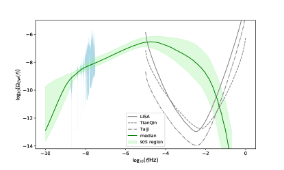
Figure 1: The expected SGWB spectrum $\Omega_{\rm{GW}}(f)$ from the SMBHBs in the frequency range $[10^{-10},10^{-1}]\rm{Hz}$. The light-blue violin plots show the posterior of the first 14-frequency bins for the NANOGrav 15-year data set. The green line shows the medium spectrum obtained from the NANOGrav analysis based on the astro-informed formation model, and the light-green shaded region indicates the $90\%$ credible interval. We also show the expected power-law integrated curves of LISA, TianQin and Taiji with solid, dashed, dash-dotted gray lines, respectively.

SGWB from SMBHB. The SGWB from SMBHBs is the most promising target of PTA. In general SMBHB is supposed to form following the merge of two galaxies. After galaxies merging, their central SMBHs sink into the center of the merger remnant and form a bound binary. Initially the binary orbit shrinks due to the energy and angular momentum exchanging with surrounding stars and cold gas. Then GW radiations will dominate the evolution at turn-over frequency $f_{t}$ with initial eccentricity $e_{0}$, bringing the binary to final coalescence (Dotti et al., 2012b). The spectrum of SGWB is composed from the sum of all GWs emitted by SMBHBs at a given observed frequency $f$. The present-day energy density of SGWB $\Omega_{\mathrm{GW}}(f)$ is given by (Phinney, 2001)

$$\Omega_{\mathrm{GW}}(f)=\frac{8\pi Gf}{3H_{0}^{2}c^{2}}\int dzd\mathcal{M}\frac{d^{2}n}{dzd\mathcal{M}}\frac{dE_{\rm GW}}{df_{r}},$$ (1)

where $H_{0}=67.4\ {\rm km\ sec^{-1}\ Mpc^{-1}}$ (Aghanim et al., 2020) is the Hubble constant, $f_{r}=(1+z)f$ is the source-frame GW frequency. Here, $\mathcal{M}=Mq^{3/5}/(1+q)^{1/5}$ is the chirp mass of SMBHB, where $M$ is the primary mass and $q$ is the mass ratio. Also, $d^{2}n/dzd\mathcal{M}$ is the SMBHB population and ${dE_{\rm GW}}/{df_{r}}$ is the energy spectrum of a single SMBHB. The relevant ranges in the integrals used here are $0\leq z\leq 5$ and $10^{5}M_{\odot}\leq\mathcal{M}\leq 10^{11}M_{\odot}$.

The SMBHB population ${d^{2}n}/{dzd\mathcal{M}}$ in Eq. (1) are estimated from astrophysical observation (Sesana et al., 2009)

$$\frac{d^{2}n}{dz^{\prime}d\mathcal{M}}=\int\frac{d^{3}n_{G}}{dz^{\prime}dM_{G}dq_{G}}\frac{dM_{G}}{dM}\frac{dq_{G}}{dq}\frac{dM}{d\mathcal{M}}dq,$$ (2)

where $M_{G}$ is the primary galaxy mass, $q_{G}$ is the mass ratio between the two paired galaxy, and $q=q_{G}^{\alpha_{*}}$ is integrated from $0.25$ to $1$. The galaxy mass $M_{G}$ and the black hole mass $M$ are related through the bulge mass $M_{\rm{bulge}}$ (Sesana, 2013; Kormendy and Ho, 2013b),

$$\frac{M_{\rm bulge}}{M_{G}}=\left\{\begin{array}[]{lr}\frac{\sqrt{6.9}}{(\log_{10}M_{G}-10)^{1.5}}\exp\left(\frac{-3.45}{\log_{10}M_{G}-10}\right)+0.615&\quad{\rm if}\log_{10}M_{G}\geq 10,\\ 0.615&\quad{\rm if}\log_{10}M_{G}\leq 10.\end{array}\right.$$ (3)

Note that this relation is only valid for red galaxy pairs which completely dominated the SGWB in PTA bands (Sesana, 2013). The primary mass $M$ is given by

$$M=\mathcal{N}\left\{M_{*}\left(\frac{M_{\rm bulge}}{10^{11}M_{\odot}}\right),\epsilon\right\},$$ (4)

with $\mathcal{N}\{x,y\}$ a log normal distribution with mean $x$ and standard deviation $y$. Here $\epsilon$ is the scatter for $M_{\rm bulge}$-$M_{\rm BH}$ relation.

The galaxy differential merger rate per unit redshift, galaxy mass and mass ratio ${d^{3}n_{G}}/{dz^{\prime}dM_{G}dq_{G}}$ is (Sesana et al., 2009)

$$\frac{d^{3}n_{G}}{dz^{\prime}dM_{G}dq_{G}}=\frac{\Phi(M_{G},z)}{M_{G}\ln 10}\frac{\mathcal{F}(M_{G},z,q_{G})}{\tau(M_{G},z,q_{G})}\frac{dt_{r}}{dz},$$ (5)

where $z$ stands for the redshift of galaxy pair, $z^{\prime}$ is the redshift at galaxy pair merging, and they are connected by merger timescale of the pair galaxy $\tau(M_{G},z,q_{G})$. The quantitative relation between $z$ and $z^{\prime}$ is addressed as (Chen et al., 2019)

$$\int_{z^{\prime}}^{z}\frac{dt}{d\tilde{z}}d\tilde{z}=\tau(M_{G},z,q_{G}).$$ (6)

Furthermore, $dt_{r}/dz$ is the relationship between time and redshift assuming a flat $\Lambda$CDM Universe

$$\frac{dt_{r}}{dz}=\frac{1}{H_{0}(1+z)\sqrt{\Omega_{M}(1+z)^{3}+\Omega_{\Lambda}}},$$ (7)

and $\Phi(M_{G},z)\equiv{dn_{G}}/{d\log_{10}M_{G}}$ is a single Schechter function describing the galaxy stellar mass function (GSMF) measured at redshift $z$ for galaxy pair, and is given by (Mortlock et al., 2015; Conselice et al., 2016)

$$\Phi(M_{G},z)=10^{\Phi(z)}(\ln 10)\left(\frac{M_{G}}{M_{G0}}\right)^{1+\alpha(z)}\exp{\left(-\frac{M_{G}}{M_{G0}}\right)},$$ (8)

where $\Phi(z)=\Phi_{0}+z\Phi_{I}$, and $\alpha(z)=\alpha_{0}+z\alpha_{I}$. The differential pair fraction with respect to the mass ratio of galaxy pair $q_{G}$ is (Chen et al., 2019)

$$\mathcal{F}(M_{G},z,q_{G})=\frac{df_{\rm pair}}{dq_{G}}=f_{0}^{\prime}\left(\frac{M_{G}}{aM_{G0}}\right)^{\alpha_{f}}\left(1+z\right)^{\beta_{f}}q_{G}^{\gamma_{f}},$$ (9)

where $aM_{G0}=10^{11}M_{\odot}$ is an arbitrary reference mass (Chen et al., 2019). Here, $f_{0}^{\prime}$ is related to $f_{0}$ via $f_{0}=f_{0}^{\prime}\int q_{G}^{\gamma_{f}}dq_{G}$. The merger timescale of the pair galaxy in Eq. (5), $\tau(M_{G},z,q_{G})$, can be expressed as (Snyder et al., 2017)

$$\tau(M_{G},z,q_{G})=\tau_{0}\left(\frac{M_{G}}{bM_{G0}}\right)^{\alpha_{\tau}}\left(1+z\right)^{\beta_{\tau}}q_{G}^{\gamma_{\tau}},$$ (10)

where $\tau_{0}$ represents merger time normalization with unit of $\rm{Gyr}$. Meanwhile, $bM_{G0}=0.4/h_{0}\times 10^{11}M_{\odot}$ is an arbitrary reference mass. Noted the merger timescale describes the time elapsed between the observed galaxy pair and the final coalescence of the SMBHB, including the time for two galaxies to effectively merge, and the time required for the SMBHs to form a binary and merge (Chen et al., 2019).

The energy spectrum of a single SMBHB $dE_{\rm GW}/df_{r}$ in Eq. (1) can be calculated using its self-similarity. In other words, a purely GW emission-driven binary spectrum in any configuration can be obtained from a reference spectrum by shift and re-scaling (Chen et al., 2017a). The fiducial redshift and chirp mass of reference spectrum are set as $z_{0}=0.02$ and $\mathcal{M}_{0}=4.16\times 10^{8}M_{\odot}$, respectively.

Here, we consider a realistic insprial phase that evolves with an initial eccentricity, and the inspiral-merger-cutoff phases are jointed smoothly following methods proposed by (Poisson, 1993; Finn and Chernoff, 1993; Zhu et al., 2011; Chen et al., 2017a). We express the complete description of energy spectrum $dE_{\rm GW}/{df_{r}}$ as follow

$$\frac{dE_{\rm GW}}{df_{r}}(f_{r}<\nu_{1}) = \frac{\pi c^{2}f}{4G}h^{2}_{\rm c,fit}\left(f\frac{f_{\rm p,\rm{ref}}}{f_{\rm p,t}}\right)\left(\frac{f_{\rm p,\rm{ref}}}{f_{\rm p,t}}\right)^{-\frac{4}{3}}$$ (11)

$$\times\left(\frac{\mathcal{M}}{\mathcal{M}_{0}}\right)^{\frac{5}{3}}\left(\frac{1+z}{1+z_{0}}\right)^{-\frac{1}{3}},$$

$$\frac{dE_{\rm GW}}{df_{r}}(f_{r}\in[\nu_{1},\nu_{2})) = \frac{(G\pi)^{2/3}\mathcal{M}^{5/3}}{3}\omega_{1}f_{r}^{2/3},$$ (12)

$$\frac{dE_{\rm GW}}{df_{r}}(f_{r}\in[\nu_{2},\nu_{3})) = \frac{(G\pi)^{2/3}\mathcal{M}^{5/3}}{3}\omega_{2}\left[\frac{f_{r}}{1+(\frac{f_{r}-\nu_{2}}{\sigma/2})^{2}}\right]^{2},$$

where $\omega_{1}=\nu_{1}^{-1}$, and $\omega_{2}=\nu_{1}^{-1}\nu_{2}^{-4/3}$. The set of parameters $(\nu_{1},\nu_{2},\sigma,\nu_{3})$ can be determined by the total mass $M_{\rm total}=M(1+q)$ and the symmetric mass ratio $\eta=(qM^{2}/M_{\rm total}^{2})$ in terms of $(a\eta^{2}+b\eta+c)/(\pi GM_{\rm total}/c^{3})$, with coefficients $a,b,c$ given in Table 1 of  (Ajith et al., 2008). The ratio ${f_{\rm p,ref}}/{f_{\rm p,t}}$ for shift is (Chen et al., 2017a)

$$\frac{f_{\rm p,{\rm ref}}}{f_{\rm p,t}}=\frac{f_{\rm ref}}{f_{t}}\left[\left(\frac{e_{\rm ref}}{e_{0}}\right)^{\frac{12}{19}}\frac{1-e_{0}^{2}}{1-e_{\rm ref}^{2}}\left(\frac{304+{121e_{\rm ref}^{2}}}{304+{121e_{0}^{2}}}\right)^{\frac{870}{2299}}\right]^{\frac{3}{2}},$$ (14)

where $f_{\rm ref}=10^{-10}{\rm Hz}$ and $e_{\rm ref}=0.9$ are the reference frequency and ecctricity, respectively. Here, $e_{0}$ is the initial eccentricity when GWs begin to dominate and $f_{t}$ is the turn-over frequency given by

$$f_{t}=0.356{\rm nHz}\left(\frac{\rho_{i,100}}{F(e_{0})\sigma_{200}}\zeta_{0}\right)^{\frac{3}{10}}\mathcal{M}_{9}^{-\frac{2}{5}},$$ (15)

where

$$F(e)=\frac{1+(73/24)e^{2}+(37/96)e^{4}}{(1-e^{2})^{7/2}},$$ (16)

$\mathcal{M}_{9}=\mathcal{M}/(10^{9}M_{\odot})$ is the rescaled chirp mass, $\rho_{i,100}=\rho_{i}/(100\,M_{\odot}\,\mathrm{pc}^{-3})$ is density of the stellar environment at the influence radius of the SMBHB, $\sigma_{200}=\sigma/(200\,\rm{km/s})$ is the velocity dispersion of stars in the galaxy, and $\zeta_{0}$ is an additional multiplicative factor absorbing all systematic uncertainties in the estimate of $\rho_{i,100}$ and $\sigma_{200}$. Note that massive galaxies generally have velocity dispersions in the range of $250\,\mathrm{km/s}<\sigma<350\,\mathrm{km/s}$, and such a narrow range has a negligible influence on the results. The analytical fitting function of spectrum, $h^{2}_{\rm c,fit}(f)$, takes the form as (Chen et al., 2017a)

$$h_{\rm c,fit}(f)=a_{0}\bar{f}^{a_{1}}e^{-a_{2}\bar{f}}+b_{0}\bar{f}^{b_{1}}e^{-b_{2}\bar{f}}+c_{0}\bar{f}^{-c_{1}}e^{-c_{2}/\bar{f}},$$ (17)

where $\bar{f}=f/(10^{-8}){\rm Hz}$, and the values of $a_{i},b_{i},c_{i}$ can given below Equation 15 in Ref. (Chen et al., 2017a).

To sum up, the present-day energy density $\Omega_{\mathrm{GW}}(f)$ of SGWB from SMBHBs in astro-informed formation model is fully specified by a set of eighteen model parameters: $\{\Phi_{0},\Phi_{I},M_{G0},\alpha_{0},\alpha_{I}\}$ for the GSMF, $\{f_{0},\alpha_{f},\beta_{f},\gamma_{f}\}$ for the pair fraction, $\{\tau_{0},\alpha_{\tau},\beta_{\tau},\gamma_{\tau}\}$ for the merger timescale, $\{M_{*},\alpha_{*},\epsilon\}$ for galaxy-SMBH transforming relation and $\{e_{0},\zeta_{0}\}$ for single SMBHB energy spectrum. The detailed descriptions of parameters are addressed in Table 1.

Table 1: List of the 18 parameters and their prior in the astro-informed formation model. Here U represents a uniform distribution.

parameter	description	prior
	GSMF
$\Phi_{0}$	GSMF norm	$-2.77_{-0.29}^{+0.27}$
$\Phi_{I}$	GSMF norm redshift evolution	$-0.27_{-0.21}^{+0.23}$
$\log_{10}M_{G0}$	GSMF scaling mass	$11.24_{-0.17}^{+0.20}$
$\alpha_{0}$	GSMF mass slope	$-1.24_{-0.16}^{+0.16}$
$\alpha_{I}$	GSMF mass slope redshift evolution	$-0.03_{-0.14}^{+0.16}$
	Galaxy pair function
$f_{0}$	pair fraction norm	U$[0.01,0.05]$
$\alpha_{f}$	pair fraction mass slope	U$[-0.5,0.5]$
$\beta_{f}$	pair fraction redshift slope	U$[0,2]$
$\gamma_{f}$	pair fraction mass ratio slope	U$[-0.2,0.2]$
	Galaxy merger timescale
$\tau_{0}$	merger time norm	U$[0.1,10]$
$\alpha_{\tau}$	merger time mass slope	U$[-0.5,0.5]$
$\beta_{\tau}$	merger time redshift slope	U$[-3,1]$
$\gamma_{\tau}$	merger time mass ratio slope	U$[-0.2,0.2]$
	$\bm{M_{\rm bulge}}$-$\bm{M_{\rm BH}}$ relation
$\log_{10}M_{*}$	$M_{\rm bulge}$-$M_{\rm BH}$ relation norm	$8.17_{-0.32}^{+0.35}$
$\alpha_{*}$	$M_{\rm bulge}$-$M_{\rm BH}$ relation slope	$1.01_{-0.10}^{+0.08}$
$\epsilon$	$M_{\rm bulge}$-$M_{\rm BH}$ relation scatter	U$[0.2,0.5]$
	Stellar and SMBHB condition
$e_{0}$	SMBHB initial eccentricity	U$[0.01,0.99]$
$\log_{10}\zeta_{0}$	stellar density factor	U$[-2,2]$

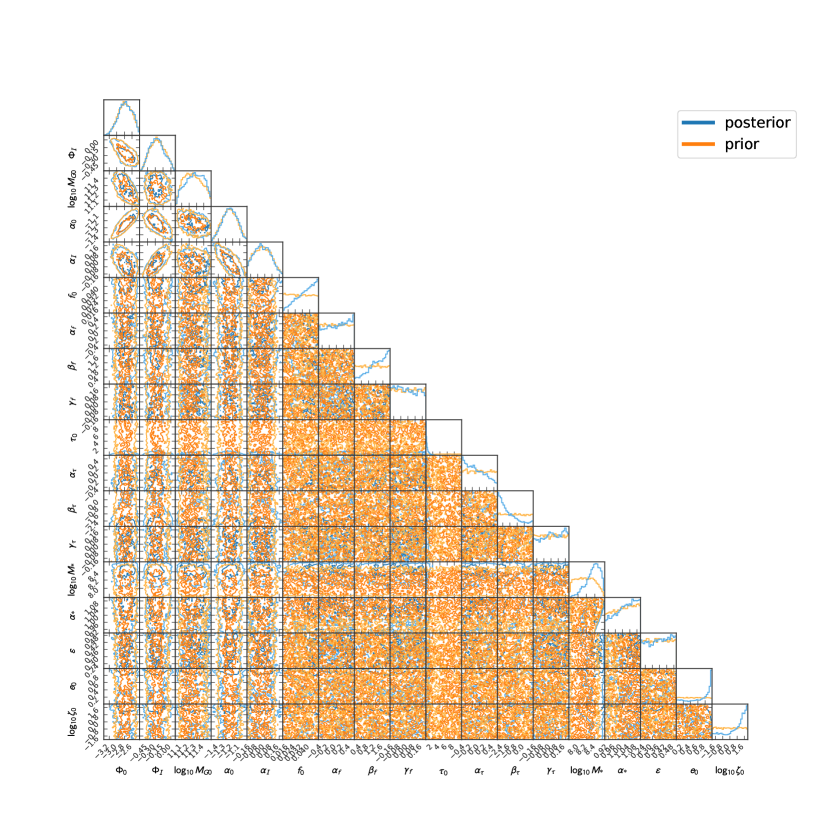
Figure 2: One- and two-dimensional prior distribution (in the orange color) and marginalised posterior distribution (in the blue color) for the 18 parameters in the astro-informed formation model. We show the $1\sigma$ and $2\sigma$ contours in the two-dimensional plots.

Data and results. The NANOGrav collaboration has performed an analysis on their 15-year data set by employing a free spectrum that enables independent variations in the amplitude of the GW spectrum across different frequencies. In the analyses, we use the posterior data from NANOGrav (Agazie et al., 2023b; Afzal et al., 2023b), and the PTMCMCSampler (Ellis and van Haasteren, 2017) package to perform the Markov Chain Monte Carlo sampling. We note that the constrained prior distributions for certain model parameters in Table 1 are based on those presented in (Chen et al., 2019) and are derived from observational and theoretical works on the measurement of the GSMF, galaxy pair fraction, merger timescale and SMBH-host galaxy scaling relations.

The resulting posterior distribution is illustrated in Fig. 2. Some parameters are prior dominated. However, our analysis also reveals that the detected stochastic signal provides some new insights into the differential pair fraction $\mathcal{F}(M_{G},z,q_{G})$, merger timescale $\tau({M_{G}},z,q_{G})$, galaxy-SMBH mass scaling $M_{G}-M_{\rm{bulge}}-M$ relation, and the initial states of the SMBHBs when GW emission takes over, such as the eccentricity $e_{0}$ and the transition frequency $f_{t}$, compared to other astrophysical observations. Specifically, the preference for a higher value of the parameter $f_{0}$ and the positive-skewed parameters $\alpha_{f}$ and $\beta_{f}$ suggest larger differential pair fractions in more massive galaxies, while the preference for a lower value of the parameter $\tau_{0}$ and the negative-skewed parameters $\alpha_{\tau}$ and $\beta_{\tau}$ indicate shorter merger timescales in more massive galaxies, and the preference for a higher value of $M_{*}$ corresponds to a higher normalization between the galaxy bulge mass $M_{\text{bulge}}$ and SMBH mass $M$. The above parameters entirely contribute to the observed relatively high amplitude of the SGWB spectrum ($\Omega_{\rm{GW}}=0.93^{+1.17}_{-0.41}\times 10^{-8}$ at $\text{yr}^{-1}=1/\text{year}$). Note that the posterior distributions of these parameters are very similar to those reported in (Middleton et al., 2021), where the NANOGrav 12.5-year data set was used. This is because the spectrum amplitudes in both data sets are statistically consistent. On the other hand, the parameters $e_{0}$ and $\zeta_{0}$, which determine the shape of the SGWB spectrum, display sharp contrasts in the posteriors obtained from the two data sets, mainly due to the fact that the two data sets are not fully statistically consistent in their measurement of spectrum shape. For the NANOGrav 15-year data set, the distribution of $e_{0}$ indicates that SMBHs exhibit a large initial eccentricity when transitioning into the GW-emission dominated process, while the larger value of the parameter $\zeta_{0}$ implies that massive galaxies have, on average, higher densities than what is suggested by a standard Dehnen profile (Dehnen, 1993).

Implication for space-borne GW detectors. In the PTA frequency band, SMBHBs are in the inspiral phase, and their radiation power can be calculated using Eq. (11). After a prolonged period of mutual inspiral, these binaries gradually transition to more circular orbits and enter the merge and ringdown phase, characterized by GW radiation described by Eq. (12) and Eq. (Implications for the Supermassive Black Hole Binaries from the NANOGrav 15-year Data Set). Some of these black holes undergo merger and final coalescence at higher frequencies, entering the space-borne GW detector frequency band. Now we can deduce the properties of the SMBHB population from the PTA results, and further combine Eq. (1) with Eqs. (11-Implications for the Supermassive Black Hole Binaries from the NANOGrav 15-year Data Set) to obtain the full SGWB spectrum generated by SMBHBs spanning both the PTA and LISA/Taiji/TianQin frequency bands, as depicted in Fig. 1.

The relation between merger rate and SMBHB chirp mass is illustrated in Fig. 3. Noted that the merger rate can be obtained from Eq.(2) in (Steinle et al., 2023) based on our population model. Essentially, the GW frequency of merging SMBHBs with total masses of $10^{4}-10^{7}M_{\odot}$ falls squarely within space-borne GW detector’s bandwidth in the late inspiral, merger and ringdown phase of the binary evolution (Colpi et al., 2019). The total mass ranges approximately correspond with $10^{5}-10^{7}M_{\odot}$ in chirp mass. Based on the posterior we obtained, the merger rate of SMBHBs with chirp masses in the range $10^{5}-10^{7}M_{\odot}$ is estimated as $\mathcal{R}\simeq 0.54_{-0.52}^{+13.05}$ yr^-1.

We need to emphasize that the general consensus for the GW detection of the cosmic history of SMBHBs is that PTAs primarily detect the SGWB from the ensemble of the SMBHB population, while LISA/Taiji/TianQin is expected to detect the final coalescence stage of individual systems. However, during the initial stages of the detector in operation, we cannot directly resolve individual sources, and it is reasonable to consider these sources as constituting an SGWB. In fact, as depicted in Fig. 1, the spectrum of the SGWB is sufficiently strong that it is very likely to be detected very soon once the detectors are in operation.

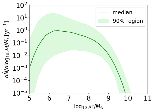
Figure 3: Posterior distributions of the SMBHB merger rate per year per unit logarithmic chirp mass over the range $\mathcal{M}\in[10^{5},10^{11}]M_{\odot}$ where the redshift is integrated over $[0,5]$. The solid line is the median and the shaded region represents the $90\%$ credible region.

Summary. In this letter, we utilize the NANOGrav 15-year data set to constrain the parameters in the astro-informed formation model for SMBHBs, implying that the SMBHBs tend to have a large initial eccentricity in the transition phase between interaction domination and GW domination. The SGWB spectrum from SMBHBs is extrapolated from the PTA frequency band to the space-borne GW detector frequency band. Our results indicate that the forthcoming LISA/Taiji/TianQin will likely detect such an SGWB from SMBHBs in the near future.

By incorporating the evolution of SMBHBs in galaxies with realistic property distributions, we combine astrophysical observations from luminosity and SGWB from PTAs. The GSMF function we used remains valid until $z<8$ and forms a solid foundation for our entire model. The posterior on GSMF aligns with the prior obtained from (Conselice et al., 2016; Chen et al., 2019). The constraints on the galaxy pair function and merger timescale are similar to those in (Middleton et al., 2021; Steinle et al., 2023). Noted that the merger timescale characterizes the galaxy merger originally. Here, we assume that any additional delay between the galaxy merger and SMBHBs merger will be absorbed in the parameter described by Eq. (10) as stated in (Chen et al., 2019).

Note that the astro-informed formation model we used is somewhat idealized. Our result is inferred by a particular black hole-galaxy population model which predicts a high IMBH number density. To obtain an accurate SGWB energy spectrum, we need a more sophisticated population model. Although there is still much work to be done, our work represents an important step forward in this endeavor.

Acknowledgements. We acknowledge the use of HPC Cluster of ITP-CAS. QGH is supported by the grants from NSFC (Grant No. 12250010, 11975019, 11991052, 12047503), Key Research Program of Frontier Sciences, CAS, Grant No. ZDBS-LY-7009, CAS Project for Young Scientists in Basic Research YSBR-006, the Key Research Program of the Chinese Academy of Sciences (Grant No. XDPB15). ZCC is supported by the National Natural Science Foundation of China (Grant No. 12247176 and No. 12247112) and the China Postdoctoral Science Foundation Fellowship No. 2022M710429.

References

- Foster and Backer (1990) R. S. Foster and D. C. Backer, “Constructing a Pulsar Timing Array,” Astrophys. J. 361, 300 (1990).
- Agazie et al. (2023a) Gabriella Agazie et al. (NANOGrav), “The NANOGrav 15-year Data Set: Observations and Timing of 68 Millisecond Pulsars,” Astrophys. J. Lett. 951 (2023a), 10.3847/2041-8213/acda9a, arXiv:2306.16217 [astro-ph.HE] .
- Agazie et al. (2023b) Gabriella Agazie et al. (NANOGrav), “The NANOGrav 15-year Data Set: Evidence for a Gravitational-Wave Background,” (2023b), 10.3847/2041-8213/acdac6, arXiv:2306.16213 [astro-ph.HE] .
- Antoniadis et al. (2023a) J. Antoniadis et al., “The second data release from the European Pulsar Timing Array I. The dataset and timing analysis,” (2023a), 10.1051/0004-6361/202346841, arXiv:2306.16224 [astro-ph.HE] .
- Antoniadis et al. (2023b) J. Antoniadis et al., “The second data release from the European Pulsar Timing Array III. Search for gravitational wave signals,” (2023b), arXiv:2306.16214 [astro-ph.HE] .
- Zic et al. (2023) Andrew Zic et al., “The Parkes Pulsar Timing Array Third Data Release,” (2023), arXiv:2306.16230 [astro-ph.HE] .
- Reardon et al. (2023) Daniel J. Reardon et al., “Search for an isotropic gravitational-wave background with the Parkes Pulsar Timing Array,” Astrophys. J. Lett. 951 (2023), 10.3847/2041-8213/acdd02, arXiv:2306.16215 [astro-ph.HE] .
- Xu et al. (2023) Heng Xu et al., “Searching for the nano-Hertz stochastic gravitational wave background with the Chinese Pulsar Timing Array Data Release I,” (2023), 10.1088/1674-4527/acdfa5, arXiv:2306.16216 [astro-ph.HE] .
- Hellings and Downs (1983) R. w. Hellings and G. s. Downs, “UPPER LIMITS ON THE ISOTROPIC GRAVITATIONAL RADIATION BACKGROUND FROM PULSAR TIMING ANALYSIS,” Astrophys. J. Lett. 265, L39–L42 (1983).
- Kibble (1976) T. W. B. Kibble, “Topology of Cosmic Domains and Strings,” J. Phys. A 9, 1387–1398 (1976).
- Vilenkin (1985) Alexander Vilenkin, “Cosmic Strings and Domain Walls,” Phys. Rept. 121, 263–315 (1985).
- Damour and Vilenkin (2005) Thibault Damour and Alexander Vilenkin, “Gravitational radiation from cosmic (super)strings: Bursts, stochastic background, and observational windows,” Phys. Rev. D 71, 063510 (2005), arXiv:hep-th/0410222 .
- Siemens et al. (2007) Xavier Siemens, Vuk Mandic, and Jolien Creighton, “Gravitational wave stochastic background from cosmic (super)strings,” Phys. Rev. Lett. 98, 111101 (2007), arXiv:astro-ph/0610920 .
- Caprini et al. (2010) Chiara Caprini, Ruth Durrer, and Xavier Siemens, “Detection of gravitational waves from the QCD phase transition with pulsar timing arrays,” Phys. Rev. D 82, 063511 (2010), arXiv:1007.1218 [astro-ph.CO] .
- Kobakhidze et al. (2017) Archil Kobakhidze, Cyril Lagger, Adrian Manning, and Jason Yue, “Gravitational waves from a supercooled electroweak phase transition and their detection with pulsar timing arrays,” Eur. Phys. J. C 77, 570 (2017), arXiv:1703.06552 [hep-ph] .
- Arunasalam et al. (2018) Suntharan Arunasalam, Archil Kobakhidze, Cyril Lagger, Shelley Liang, and Albert Zhou, “Low temperature electroweak phase transition in the Standard Model with hidden scale invariance,” Phys. Lett. B 776, 48–53 (2018), arXiv:1709.10322 [hep-ph] .
- Xue et al. (2021) Xiao Xue et al., “Constraining Cosmological Phase Transitions with the Parkes Pulsar Timing Array,” Phys. Rev. Lett. 127, 251303 (2021), arXiv:2110.03096 [astro-ph.CO] .
- Maggiore (2000) Michele Maggiore, “Gravitational wave experiments and early universe cosmology,” Phys. Rept. 331, 283–367 (2000), arXiv:gr-qc/9909001 .
- Saito and Yokoyama (2009) Ryo Saito and Jun’ichi Yokoyama, “Gravitational wave background as a probe of the primordial black hole abundance,” Phys. Rev. Lett. 102, 161101 (2009), [Erratum: Phys.Rev.Lett. 107, 069901 (2011)], arXiv:0812.4339 [astro-ph] .
- Caprini and Figueroa (2018) Chiara Caprini and Daniel G. Figueroa, “Cosmological Backgrounds of Gravitational Waves,” Class. Quant. Grav. 35, 163001 (2018), arXiv:1801.04268 [astro-ph.CO] .
- Chen et al. (2020) Zu-Cheng Chen, Chen Yuan, and Qing-Guo Huang, “Pulsar Timing Array Constraints on Primordial Black Holes with NANOGrav 11-Year Dataset,” Phys. Rev. Lett. 124, 251101 (2020), arXiv:1910.12239 [astro-ph.CO] .
- Cai et al. (2020) Rong-Gen Cai, Zong-Kuan Guo, Jing Liu, Lang Liu, and Xing-Yu Yang, “Primordial black holes and gravitational waves from parametric amplification of curvature perturbations,” JCAP 06, 013 (2020), arXiv:1912.10437 [astro-ph.CO] .
- Yuan et al. (2020a) Chen Yuan, Zu-Cheng Chen, and Qing-Guo Huang, “Scalar induced gravitational waves in different gauges,” Phys. Rev. D 101, 063018 (2020a), arXiv:1912.00885 [astro-ph.CO] .
- Li et al. (2019) Jun Li, Zu-Cheng Chen, and Qing-Guo Huang, “Measuring the tilt of primordial gravitational-wave power spectrum from observations,” Sci. China Phys. Mech. Astron. 62, 110421 (2019), [Erratum: Sci.China Phys.Mech.Astron. 64, 250451 (2021)], arXiv:1907.09794 [astro-ph.CO] .
- Yuan et al. (2020b) Chen Yuan, Zu-Cheng Chen, and Qing-Guo Huang, “Log-dependent slope of scalar induced gravitational waves in the infrared regions,” Phys. Rev. D 101, 043019 (2020b), arXiv:1910.09099 [astro-ph.CO] .
- Yuan et al. (2019) Chen Yuan, Zu-Cheng Chen, and Qing-Guo Huang, “Probing primordial–black-hole dark matter with scalar induced gravitational waves,” Phys. Rev. D 100, 081301 (2019), arXiv:1906.11549 [astro-ph.CO] .
- Liu et al. (2023a) Lang Liu, Xing-Yu Yang, Zong-Kuan Guo, and Rong-Gen Cai, “Testing primordial black hole and measuring the Hubble constant with multiband gravitational-wave observations,” JCAP 01, 006 (2023a), arXiv:2112.05473 [astro-ph.CO] .
- Chen et al. (2022a) Zu-Cheng Chen, Yu-Mei Wu, and Qing-Guo Huang, “Searching for isotropic stochastic gravitational-wave background in the international pulsar timing array second data release,” Commun. Theor. Phys. 74, 105402 (2022a), arXiv:2109.00296 [astro-ph.CO] .
- Moore and Vecchio (2021) Christopher J. Moore and Alberto Vecchio, “Ultra-low-frequency gravitational waves from cosmological and astrophysical processes,” Nature Astron. 5, 1268–1274 (2021), arXiv:2104.15130 [astro-ph.CO] .
- Wu et al. (2022a) Yu-Mei Wu, Zu-Cheng Chen, and Qing-Guo Huang, “Constraining the Polarization of Gravitational Waves with the Parkes Pulsar Timing Array Second Data Release,” Astrophys. J. 925, 37 (2022a), arXiv:2108.10518 [astro-ph.CO] .
- Chen et al. (2021) Zu-Cheng Chen, Chen Yuan, and Qing-Guo Huang, “Non-tensorial gravitational wave background in NANOGrav 12.5-year data set,” Sci. China Phys. Mech. Astron. 64, 120412 (2021), arXiv:2101.06869 [astro-ph.CO] .
- Wu et al. (2022b) Yu-Mei Wu, Zu-Cheng Chen, Qing-Guo Huang, Xingjiang Zhu, N. D. Ramesh Bhat, Yi Feng, George Hobbs, Richard N. Manchester, Christopher J. Russell, and R. M. Shannon (PPTA), “Constraining ultralight vector dark matter with the Parkes Pulsar Timing Array second data release,” Phys. Rev. D 106, L081101 (2022b), arXiv:2210.03880 [astro-ph.CO] .
- Chen et al. (2022b) Zu-Cheng Chen, Yu-Mei Wu, and Qing-Guo Huang, “Search for the Gravitational-wave Background from Cosmic Strings with the Parkes Pulsar Timing Array Second Data Release,” Astrophys. J. 936, 20 (2022b), arXiv:2205.07194 [astro-ph.CO] .
- Bian et al. (2022) Ligong Bian, Jing Shu, Bo Wang, Qiang Yuan, and Junchao Zong, “Searching for cosmic string induced stochastic gravitational wave background with the Parkes Pulsar Timing Array,” Phys. Rev. D 106, L101301 (2022), arXiv:2205.07293 [hep-ph] .
- Meng et al. (2023) De-Shuang Meng, Chen Yuan, and Qing-Guo Huang, “Primordial black holes generated by the non-minimal spectator field,” Sci. China Phys. Mech. Astron. 66, 280411 (2023), arXiv:2212.03577 [astro-ph.CO] .
- Chen et al. (2022c) Zu-Cheng Chen, Chen Yuan, and Qing-Guo Huang, “Confronting the primordial black hole scenario with the gravitational-wave events detected by LIGO-Virgo,” Phys. Lett. B 829, 137040 (2022c), arXiv:2108.11740 [astro-ph.CO] .
- Afzal et al. (2023a) Adeela Afzal et al. (NANOGrav), “The NANOGrav 15 yr Data Set: Search for Signals from New Physics,” Astrophys. J. Lett. 951, L11 (2023a), arXiv:2306.16219 [astro-ph.HE] .
- Wu et al. (2023a) Yu-Mei Wu, Zu-Cheng Chen, and Qing-Guo Huang, “Pulsar timing residual induced by ultralight tensor dark matter,” (2023a), arXiv:2305.08091 [hep-ph] .
- Wu et al. (2023b) Yu-Mei Wu, Zu-Cheng Chen, and Qing-Guo Huang, “Search for stochastic gravitational-wave background from massive gravity in the NANOGrav 12.5-year dataset,” Phys. Rev. D 107, 042003 (2023b), arXiv:2302.00229 [gr-qc] .
- Wu et al. (2023c) Yu-Mei Wu, Zu-Cheng Chen, and Qing-Guo Huang, “Cosmological Interpretation for the Stochastic Signal in Pulsar Timing Arrays,” (2023c), arXiv:2307.03141 [astro-ph.CO] .
- Liu et al. (2023b) Lang Liu, Zu-Cheng Chen, and Qing-Guo Huang, “Implications for the non-Gaussianity of curvature perturbation from pulsar timing arrays,” (2023b), arXiv:2307.01102 [astro-ph.CO] .
- Guo et al. (2023) Shu-Yuan Guo, Maxim Khlopov, Xuewen Liu, Lei Wu, Yongcheng Wu, and Bin Zhu, “Footprints of Axion-Like Particle in Pulsar Timing Array Data and JWST Observations,” (2023), arXiv:2306.17022 [hep-ph] .
- Broadhurst et al. (2023) Tom Broadhurst, Chao Chen, Tao Liu, and Kai-Feng Zheng, “Binary Supermassive Black Holes Orbiting Dark Matter Solitons: From the Dual AGN in UGC4211 to NanoHertz Gravitational Waves,” (2023), arXiv:2306.17821 [astro-ph.HE] .
- Yang et al. (2023) Jing Yang, Ning Xie, and Fa Peng Huang, “Implication of nano-Hertz stochastic gravitational wave background on ultralight axion particles,” (2023), arXiv:2306.17113 [hep-ph] .
- Konoplya and Zhidenko (2023) R. A. Konoplya and A. Zhidenko, “Asymptotic tails of massive gravitons in light of pulsar timing array observations,” (2023), arXiv:2307.01110 [gr-qc] .
- Lazarides et al. (2023) George Lazarides, Rinku Maji, and Qaisar Shafi, “Superheavy quasi-stable strings and walls bounded by strings in the light of NANOGrav 15 year data,” (2023), arXiv:2306.17788 [hep-ph] .
- King et al. (2023) Stephen F. King, Danny Marfatia, and Moinul Hossain Rahat, “Towards distinguishing Dirac from Majorana neutrino mass with gravitational waves,” (2023), arXiv:2306.05389 [hep-ph] .
- Niu and Rahat (2023) Xuce Niu and Moinul Hossain Rahat, “NANOGrav signal from axion inflation,” (2023), arXiv:2307.01192 [hep-ph] .
- Jin et al. (2023) Jia-Heng Jin, Zu-Cheng Chen, Zhu Yi, Zhi-Qiang You, Lang Liu, and You Wu, “Confronting sound speed resonance with pulsar timing arrays,” JCAP 09, 016 (2023), arXiv:2307.08687 [astro-ph.CO] .
- Madge et al. (2023) Eric Madge, Enrico Morgante, Cristina Puchades-Ibáñez, Nicklas Ramberg, Wolfram Ratzinger, Sebastian Schenk, and Pedro Schwaller, “Primordial gravitational waves in the nano-Hertz regime and PTA data – towards solving the GW inverse problem,” (2023), arXiv:2306.14856 [hep-ph] .
- Wang et al. (2023a) Sai Wang, Zhi-Chao Zhao, and Qing-Hua Zhu, “Constraints On Scalar-Induced Gravitational Waves Up To Third Order From Joint Analysis of BBN, CMB, And PTA Data,” (2023a), arXiv:2307.03095 [astro-ph.CO] .
- Wang et al. (2023b) Sai Wang, Zhi-Chao Zhao, Jun-Peng Li, and Qing-Hua Zhu, “Exploring the Implications of 2023 Pulsar Timing Array Datasets for Scalar-Induced Gravitational Waves and Primordial Black Holes,” (2023b), arXiv:2307.00572 [astro-ph.CO] .
- Li et al. (2023a) Jun-Peng Li, Sai Wang, Zhi-Chao Zhao, and Kazunori Kohri, “Primordial Non-Gaussianity and Anisotropies in Gravitational Waves induced by Scalar Perturbations,” (2023a), arXiv:2305.19950 [astro-ph.CO] .
- Wang and Zhao (2023) Sai Wang and Zhi-Chao Zhao, “Unveiling the Graviton Mass Bounds through Analysis of 2023 Pulsar Timing Array Datasets,” (2023), arXiv:2307.04680 [astro-ph.HE] .
- Addazi et al. (2023) Andrea Addazi, Yi-Fu Cai, Antonino Marciano, and Luca Visinelli, “Have pulsar timing array methods detected a cosmological phase transition?” (2023), arXiv:2306.17205 [astro-ph.CO] .
- Franciolini et al. (2023) Gabriele Franciolini, Antonio Iovino, Junior., Ville Vaskonen, and Hardi Veermae, “The recent gravitational wave observation by pulsar timing arrays and primordial black holes: the importance of non-gaussianities,” (2023), arXiv:2306.17149 [astro-ph.CO] .
- Ellis et al. (2023a) John Ellis, Marek Lewicki, Chunshan Lin, and Ville Vaskonen, “Cosmic Superstrings Revisited in Light of NANOGrav 15-Year Data,” (2023a), arXiv:2306.17147 [astro-ph.CO] .
- Bian et al. (2023) Ligong Bian, Shuailiang Ge, Jing Shu, Bo Wang, Xing-Yu Yang, and Junchao Zong, “Gravitational wave sources for Pulsar Timing Arrays,” (2023), arXiv:2307.02376 [astro-ph.HE] .
- Liu et al. (2023c) Lang Liu, Zu-Cheng Chen, and Qing-Guo Huang, “Probing the equation of state of the early Universe with pulsar timing arrays,” (2023c), arXiv:2307.14911 [astro-ph.CO] .
- Yi et al. (2023a) Zhu Yi, Zhi-Qiang You, You Wu, Zu-Cheng Chen, and Lang Liu, “Exploring the NANOGrav Signal and Planet-mass Primordial Black Holes through Higgs Inflation,” (2023a), arXiv:2308.14688 [astro-ph.CO] .
- Yi et al. (2023b) Zhu Yi, Zhi-Qiang You, and You Wu, “Model-independent reconstruction of the primordial curvature power spectrum from PTA data,” (2023b), arXiv:2308.05632 [astro-ph.CO] .
- You et al. (2023) Zhi-Qiang You, Zhu Yi, and You Wu, “Constraints on primordial curvature power spectrum with pulsar timing arrays,” (2023), arXiv:2307.04419 [gr-qc] .
- Falxa et al. (2023) M. Falxa et al. (IPTA), “Searching for continuous Gravitational Waves in the second data release of the International Pulsar Timing Array,” Mon. Not. Roy. Astron. Soc. 521, 5077–5086 (2023), arXiv:2303.10767 [gr-qc] .
- Chen et al. (2023) Zu-Cheng Chen, Qing-Guo Huang, Chang Liu, Lang Liu, Xiao-Jin Liu, You Wu, Yu-Mei Wu, Zhu Yi, and Zhi-Qiang You, “Prospects for Taiji to detect a gravitational-wave background from cosmic strings,” (2023), arXiv:2310.00411 [astro-ph.IM] .
- Agazie et al. (2023c) G. Agazie et al. (International Pulsar Timing Array), “Comparing recent PTA results on the nanohertz stochastic gravitational wave background,” (2023c), arXiv:2309.00693 [astro-ph.HE] .
- Agazie et al. (2023d) Gabriella Agazie et al. (NANOGrav), “The NANOGrav 15-year Data Set: Constraints on Supermassive Black Hole Binaries from the Gravitational Wave Background,” (2023d), arXiv:2306.16220 [astro-ph.HE] .
- Agazie et al. (2023e) Gabriella Agazie et al. (NANOGrav), “The NANOGrav 15-year Data Set: Bayesian Limits on Gravitational Waves from Individual Supermassive Black Hole Binaries,” (2023e), arXiv:2306.16222 [astro-ph.HE] .
- Antoniadis et al. (2023c) J. Antoniadis et al., “The second data release from the European Pulsar Timing Array: V. Implications for massive black holes, dark matter and the early Universe,” (2023c), arXiv:2306.16227 [astro-ph.CO] .
- Ellis et al. (2023b) John Ellis, Malcolm Fairbairn, Gert Hütsi, Juhan Raidal, Juan Urrutia, Ville Vaskonen, and Hardi Veermäe, “Gravitational Waves from SMBH Binaries in Light of the NANOGrav 15-Year Data,” (2023b), arXiv:2306.17021 [astro-ph.CO] .
- Li et al. (2023b) Zhencheng Li, Zhen Jiang, Xi-Long Fan, Yun Chen, Liang Gao, and Shenghua Yu, “Exploring the multi-band gravitational wave background with a semi-analytic galaxy formation model,” (2023b), arXiv:2304.08333 [gr-qc] .
- Begelman et al. (1980) M. C. Begelman, R. D. Blandford, and M. J. Rees, “Massive black hole binaries in active galactic nuclei,” Nature 287, 307–309 (1980).
- Dotti et al. (2012a) M. Dotti, A. Sesana, and R. Decarli, “Massive black hole binaries: dynamical evolution and observational signatures,” Adv. Astron. 2012, 940568 (2012a), arXiv:1111.0664 [astro-ph.CO] .
- Kocsis and Sesana (2011) Bence Kocsis and Alberto Sesana, “Gas driven massive black hole binaries: signatures in the nHz gravitational wave background,” Mon. Not. Roy. Astron. Soc. 411, 1467 (2011), arXiv:1002.0584 [astro-ph.CO] .
- Sesana (2013) A. Sesana, “Insights into the astrophysics of supermassive black hole binaries from pulsar timing observations,” Class. Quant. Grav. 30, 224014 (2013), arXiv:1307.2600 [astro-ph.CO] .
- Ravi et al. (2014) V. Ravi, J. S. B. Wyithe, R. M. Shannon, G. Hobbs, and R. N. Manchester, “Binary supermassive black hole environments diminish the gravitational wave signal in the pulsar timing band,” Mon. Not. Roy. Astron. Soc. 442, 56–68 (2014), arXiv:1404.5183 [astro-ph.CO] .
- Kelley et al. (2017) Luke Zoltan Kelley, Laura Blecha, and Lars Hernquist, “Massive Black Hole Binary Mergers in Dynamical Galactic Environments,” Mon. Not. Roy. Astron. Soc. 464, 3131–3157 (2017), arXiv:1606.01900 [astro-ph.HE] .
- Chen et al. (2017a) Siyuan Chen, Alberto Sesana, and Walter Del Pozzo, “Efficient computation of the gravitational wave spectrum emitted by eccentric massive black hole binaries in stellar environments,” Mon. Not. Roy. Astron. Soc. 470, 1738–1749 (2017a), arXiv:1612.00455 [astro-ph.CO] .
- Rodig et al. (2011) Constanze Rodig, Massimo Dotti, Alberto Sesana, Jorge Cuadra, and Monica Colpi, “Limiting eccentricity of sub-parsec massive black hole binaries surrounded by self-gravitating gas discs,” Mon. Not. Roy. Astron. Soc. 415, 3033 (2011), arXiv:1104.3868 [astro-ph.CO] .
- Quinlan (1996) Gerald D. Quinlan, “The dynamical evolution of massive black hole binaries - I. hardening in a fixed stellar background,” New Astron. 1, 35–56 (1996), arXiv:astro-ph/9601092 .
- Armitage and Natarajan (2005) Philip J. Armitage and Priyamvada Natarajan, “Eccentricity of supermassive black hole binaries coalescing from gas rich mergers,” Astrophys. J. 634, 921–928 (2005), arXiv:astro-ph/0508493 .
- Chen et al. (2019) Siyuan Chen, Alberto Sesana, and Christopher J. Conselice, “Constraining astrophysical observables of Galaxy and Supermassive Black Hole Binary Mergers using Pulsar Timing Arrays,” Mon. Not. Roy. Astron. Soc. 488, 401–418 (2019), arXiv:1810.04184 [astro-ph.GA] .
- Bell et al. (2006) Eric F. Bell, Stefanie Phleps, Rachel S. Somerville, Christian Wolf, Andrea Borch, and Klaus Meisenheimer, “The merger rate of massive galaxies,” Astrophys. J. 652, 270–276 (2006), arXiv:astro-ph/0602038 .
- de Ravel et al. (2009) L. de Ravel et al., “The VIMOS VLT Deep Survey :Evolution of the major merger rate since z~1 from spectroscopicaly confirmed galaxy pairs,” Astron. Astrophys. 498, 379 (2009), arXiv:0807.2578 [astro-ph] .
- Sesana et al. (2008) Alberto Sesana, Alberto Vecchio, and Carlo Nicola Colacino, “The stochastic gravitational-wave background from massive black hole binary systems: implications for observations with Pulsar Timing Arrays,” Mon. Not. Roy. Astron. Soc. 390, 192 (2008), arXiv:0804.4476 [astro-ph] .
- Kormendy and Ho (2013a) John Kormendy and Luis C. Ho, “Coevolution (Or Not) of Supermassive Black Holes and Host Galaxies,” Ann. Rev. Astron. Astrophys. 51, 511–653 (2013a), arXiv:1304.7762 [astro-ph.CO] .
- Chen et al. (2017b) Siyuan Chen, Hannah Middleton, Alberto Sesana, Walter Del Pozzo, and Alberto Vecchio, “Probing the assembly history and dynamical evolution of massive black hole binaries with pulsar timing arrays,” Mon. Not. Roy. Astron. Soc. 468, 404–417 (2017b), [Erratum: Mon.Not.Roy.Astron.Soc. 469, 2455–2456 (2017)], arXiv:1612.02826 [astro-ph.HE] .
- Amaro-Seoane et al. (2017) Pau Amaro-Seoane et al. (LISA), “Laser Interferometer Space Antenna,” (2017), arXiv:1702.00786 [astro-ph.IM] .
- Luo et al. (2020) Ziren Luo, Yan Wang, Yueliang Wu, Wenrui Hu, and Gang Jin, “The Taiji program: A concise overview,” Progress of Theoretical and Experimental Physics 2021 (2020), 10.1093/ptep/ptaa083.
- Luo et al. (2016) Jun Luo et al. (TianQin), “TianQin: a space-borne gravitational wave detector,” Class. Quant. Grav. 33, 035010 (2016), arXiv:1512.02076 [astro-ph.IM] .
- Conselice et al. (2016) Christopher J. Conselice, Aaron Wilkinson, Kenneth Duncan, and Alice Mortlock, “THE EVOLUTION OF GALAXY NUMBER DENSITY ATz 8 AND ITS IMPLICATIONS,” Astrophys. J. 830, 83 (2016).
- Kormendy and Ho (2013b) John Kormendy and Luis C. Ho, “Coevolution (Or Not) of Supermassive Black Holes and Host Galaxies,” Ann. Rev. Astron. Astrophys. 51, 511–653 (2013b), arXiv:1304.7762 [astro-ph.CO] .
- Dotti et al. (2012b) M. Dotti, A. Sesana, and R. Decarli, “Massive black hole binaries: dynamical evolution and observational signatures,” Adv. Astron. 2012, 940568 (2012b), arXiv:1111.0664 [astro-ph.CO] .
- Phinney (2001) E. S. Phinney, “A Practical theorem on gravitational wave backgrounds,” (2001), arXiv:astro-ph/0108028 .
- Aghanim et al. (2020) N. Aghanim et al. (Planck), “Planck 2018 results. VI. Cosmological parameters,” Astron. Astrophys. 641, A6 (2020), [Erratum: Astron.Astrophys. 652, C4 (2021)], arXiv:1807.06209 [astro-ph.CO] .
- Sesana et al. (2009) A. Sesana, A. Vecchio, and M. Volonteri, “Gravitational waves from resolvable massive black hole binary systems and observations with Pulsar Timing Arrays,” Mon. Not. Roy. Astron. Soc. 394, 2255 (2009), arXiv:0809.3412 [astro-ph] .
- Mortlock et al. (2015) Alice Mortlock et al., “Deconstructing the Galaxy Stellar Mass Function with UKIDSS and CANDELS: the Impact of Colour, Structure and Environment,” Mon. Not. Roy. Astron. Soc. 447, 2–24 (2015), arXiv:1411.3339 [astro-ph.GA] .
- Snyder et al. (2017) Gregory F. Snyder, Jennifer M. Lotz, Vicente Rodriguez-Gomez, Renato da Silva Guimarães, Paul Torrey, and Lars Hernquist, “Massive close pairs measure rapid galaxy assembly in mergers at high redshift,” Monthly Notices of the Royal Astronomical Society 468, 207–216 (2017).
- Poisson (1993) Eric Poisson, “Gravitational radiation from a particle in circular orbit around a black hole. 1: Analytical results for the nonrotating case,” Phys. Rev. D 47, 1497–1510 (1993).
- Finn and Chernoff (1993) Lee Samuel Finn and David F. Chernoff, “Observing binary inspiral in gravitational radiation: One interferometer,” Phys. Rev. D 47, 2198–2219 (1993), arXiv:gr-qc/9301003 .
- Zhu et al. (2011) Xing-Jiang Zhu, E. Howell, T. Regimbau, D. Blair, and Zong-Hong Zhu, “Stochastic Gravitational Wave Background from Coalescing Binary Black Holes,” Astrophys. J. 739, 86 (2011), arXiv:1104.3565 [gr-qc] .
- Ajith et al. (2008) P. Ajith et al., “A Template bank for gravitational waveforms from coalescing binary black holes. I. Non-spinning binaries,” Phys. Rev. D 77, 104017 (2008), [Erratum: Phys.Rev.D 79, 129901 (2009)], arXiv:0710.2335 [gr-qc] .
- Afzal et al. (2023b) Adeela Afzal et al. (NANOGrav), “The NANOGrav 15-year Data Set: Search for Signals from New Physics,” Astrophys. J. Lett. 951 (2023b), 10.3847/2041-8213/acdc91, arXiv:2306.16219 [astro-ph.HE] .
- Ellis and van Haasteren (2017) Justin Ellis and Rutger van Haasteren, “jellis18/ptmcmcsampler: Official release,” (2017).
- Middleton et al. (2021) H. Middleton, A. Sesana, S. Chen, A. Vecchio, W. Del Pozzo, and P. A. Rosado, “Massive black hole binary systems and the NANOGrav 12.5 yr results,” Mon. Not. Roy. Astron. Soc. 502, L99–L103 (2021), arXiv:2011.01246 [astro-ph.HE] .
- Dehnen (1993) W. Dehnen, “A Family of Potential-Density Pairs for Spherical Galaxies and Bulges,” Mon. Not. Roy. Astron. Soc. 265, 250 (1993).
- Steinle et al. (2023) Nathan Steinle, Hannah Middleton, Christopher J. Moore, Siyuan Chen, Antoine Klein, Geraint Pratten, Riccardo Buscicchio, Eliot Finch, and Alberto Vecchio, “Implications of pulsar timing array observations for LISA detections of massive black hole binaries,” (2023), arXiv:2305.05955 [astro-ph.HE] .
- Colpi et al. (2019) Monica Colpi et al., “Astro2020 science white paper: The gravitational wave view of massive black holes,” (2019), arXiv:1903.06867 [astro-ph.GA] .