marginparsep has been altered.
topmargin has been altered.
marginparpush has been altered.
The page layout violates the ICML style.
Please do not change the page layout, or include packages like geometry,
savetrees, or fullpage, which change it for you.
We’re not able to reliably undo arbitrary changes to the style. Please remove
the offending package(s), or layout-changing commands and try again.
Neural Polytopes
Koji Hashimoto 1 Tomoya Naito 2 3 Hisashi Naito 4
Accepted after peer-review at the 1st workshop on Synergy of Scientific and Machine Learning Modeling, SynS & ML ICML, Honolulu, Hawaii, USA. July, 2023. Copyright 2023 by the author(s).
Abstract
We find that simple neural networks with ReLU activation generate polytopes as an approximation of a unit sphere in various dimensions. The species of polytopes are regulated by the network architecture, such as the number of units and layers. For a variety of activation functions, generalization of polytopes is obtained, which we call neural polytopes. They are a smooth analogue of polytopes, exhibiting geometric duality. This finding initiates research of generative discrete geometry to approximate surfaces by machine learning.
Introduction
The approach humans have taken to modeling nature is to approximate smooth curved surfaces in nature with linear objects such as planes. This is natural in terms of recognizing natural objects composed of smooth curves, since the simplest solution to the equations of motion in physics is linear motion with constant velocity. In ancient Greece, polygons were discovered as a way to approximate a circle by straight line segments, and polyhedra as a way to approximate a sphere by pieces of planes, and in particular, it was assumed by Plato that the existence of only a finite number of regular polyhedra was the fundamental understanding of nature. Thus, approximating rotationally symmetric objects (circles and spheres) with piecewise linear functions is at the root of modeling nature.
Machine learning, on the other hand, is known to be able to approximate any function if the network architecture is multi-unit multilayer, as stated in the universal approximation theorem Cybenko (1989); Hornik et al. (1989); Hornik (1991). In particular, taking the activation function to be a step function or ReLU can be identified with approximation by a piecewise constant or piecewise linear function. Therefore, the modeling of approximation of natural phenomena by neural networks should naturally lead us to the rediscovery of discrete geometry, when we go back to the motivation in ancient Greek times and target the rotationally symmetric objects.
Discrete geometry is the research field in mathematics to develop methods for discretizing smooth surfaces, whose application ranges from computer graphics Baumgart (1974) to quantum physics. To cite an example of the latter, the fundamental goal of completing the quantum theory of gravity in physics is to discretely approximate and quantize a smoothly curved surface called spacetime Regge (1961). Thus, the development of methods in discrete geometry is long overdue.
In this study, a sphere is approximated by a neural network function, as a first numerical experiment to bridge discrete geometry and machine learning and to explore possible visualization of trained functions.
As we describe below, for the choice of the activation function as ReLU, polygons and polytopes are naturally generated. When we allow other activation functions, we obtain infinite families of generalization of polytopes — which we call neural polytopes.
Method
A plane in the Euclidean -dimensional space spanned by the coordinate is parameterized as
| (1) |
where (, …, ) are real constant parameters. Polyhedra are nothing but a generalization of this equation to a piecewise linear function. Note that the right-hand side of (1) needs to be fixed to be the unity; otherwise, we have to require some affine quotient.
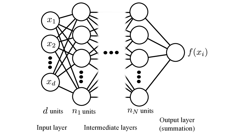
Now, we notice that any feed-forward deep neural network with the ReLU activation function without the bias is exactly of the form of the left-hand side of (1). Therefore, let us prepare a deep neural network architecture with intermediate fully-connected layers with units each, and with the ReLU activation function. The input layer consists of units whose input is just the coordinate . For simplicity, the output layer is taken to be a summation layer which sums the values of the units at the last intermediate layer. We force all biases equal to be zero. See Fig. 1 for the architecture.
The preparation of the training data is straightforward; since we aim to approximate the -sphere, we produce a set of random points on the -sphere in the Cartesian coordinates, and produce the data set of the form
| (2) |
That is, the input is a random point on the , and the output is the unity.
The activation function other than ReLU,
| (3) |
with a positive real constant , gives geometrically symmetric neural network functions, as it respects the reflection symmetry . This paper focuses on the results with (3) for a better symmetric approximation of spheres. Note that choosing results in the complete reproduction of the original sphere (circle), since the equation to define the sphere is of the symmetric quadratic functions, .
For the training, we produce roughly 10000 random points on the sphere, and use the ADAM optimizer with batch size 1000. 10000 epochs are enough for the training, as in this study we focus on very small architecture to see the discreteness of the neural network functions.111We do not show the explicit values of the loss functions after the training, as our neural network architecture is quite small in size and the minimum of the loss function landscape is expected to be unique, in all of our examples, up to the trivial flat directions generated by the rotation.
After the training, we plot the cross section defined by
| (4) |
where is the trained neural network function. We call this cross section “neural polytopes.” We name the produced polytopes as -polytope of type , where is the spatial dimension of the minimal Euclidean space in which the polytope is embedded (i.e. the number of input units), and refers to the number of units in each of the intermediate layers, and is the power appearing in the activation function at each layer. When , we just call it type .


Results
In this report, we concentrate on the symmetric activation function (3) to find rather symmetric neural polytopes.222Numerical training of the neural networks was done using Mathematica. The plots are numerical solutions of (4) in spherical coordinates. This also serves to test the “rediscovery” of regular polygons and polyhedra for our choice in the activation function.
Polygons, polyhedra and polytopes
First, we report our results for . In Fig. 2, we show the results of the neural polygons. This is the -polytopes of type . It is amusing to find that -sided regular polygons known for thousands of years are reproduced beautifully, thus establishing the map between the neural network architecture and the regular polygons.
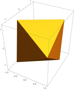
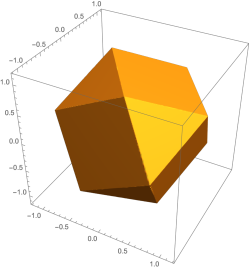
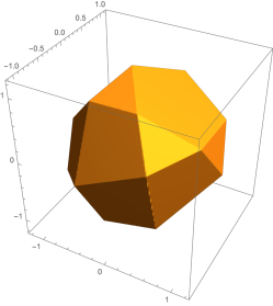
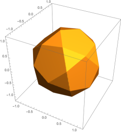
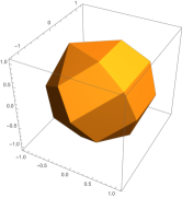
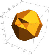
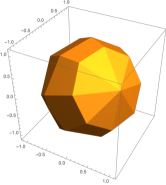
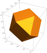
Next, we list the results of neural polyhedra. These are the neural -polytopes of type , see Fig. 3. The type is the octahedron, which is one of the regular polyhedra. The type is the cuboctahedron, and the type is the icosidodecahedron, both of which are of the Archimedean solids. It is again amusing that various truncated polyhedra show up naturally.
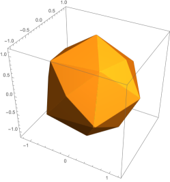
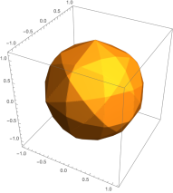
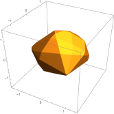
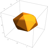
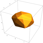
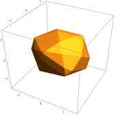
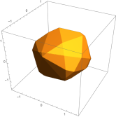
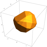
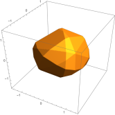
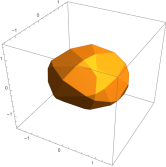
Deeper neural network approximates the sphere more efficiently, and in Fig. 4 we list the results of neural -polytope of type . Compared with type with sharing the same , we find that deeper network approximate the sphere better.
In Fig. 5, we provide a higher-dimensional example: a neural -polytope of type . The plot is various 3-dimensional slices of the 5-polytope.
Neural polytopes
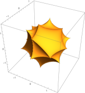
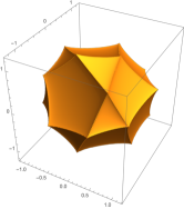
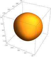
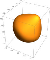
Next, let us turn to the case . Interestingly, neural polytopes with are spiky () or round () generalizations of the ordinary polytopes (). In the limit , the neural polytopes become ordinary polytopes different from those for . At , the neural polytopes are spheres.
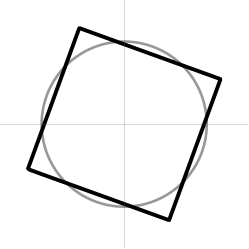
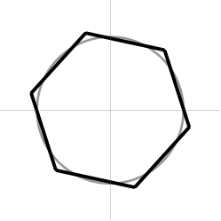
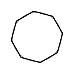
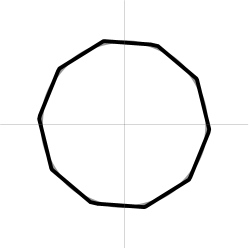
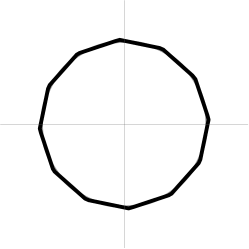
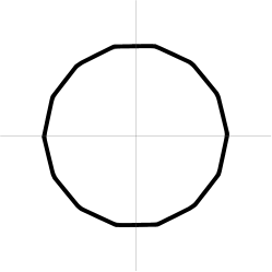
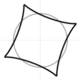
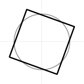
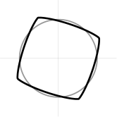
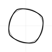
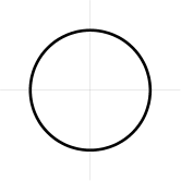
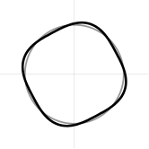
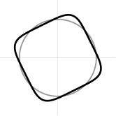
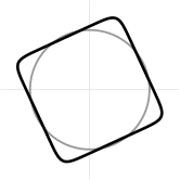
First, in Fig. 6, we show neural 2-polytopes (neural polygons) of type with , , , , , , and . At the neural polygon is a square. Increasing makes the edge vertex rounded. At the neural polygon is a circle. Then, at the neural polygon becomes again a square. The edge shape of the neural polygons is actually identical to the shape of the activation function .
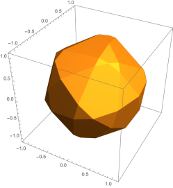
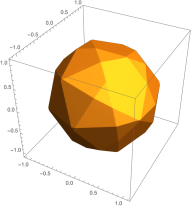
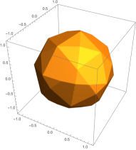
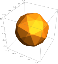
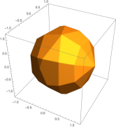
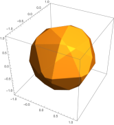
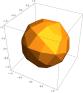
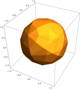
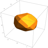
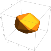
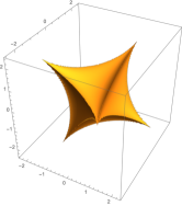
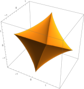
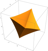
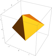
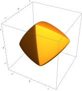
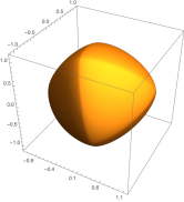
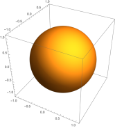
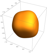
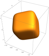
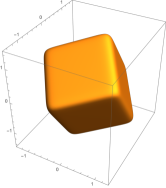
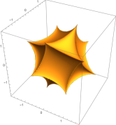
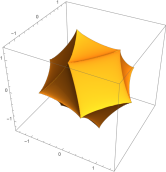
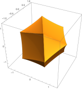
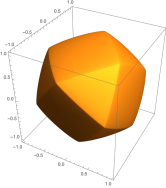
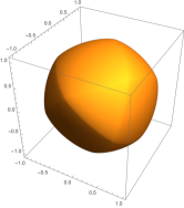
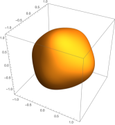
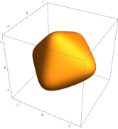
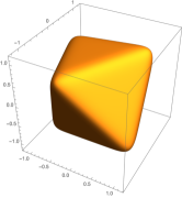
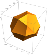
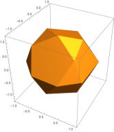
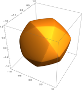
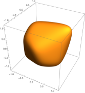
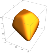
Neural 3-polytopes (neural polyhedra) are plotted in Figs. 7, 8, and 9. The behavior in change of the value of is quite similar to that of the neural polygons.
For the neural polyhedra of type , the neural polyhedron is an octahedron, while is a cube. Interestingly, these are dual polyhedra. So the and neural polyhedra provide a well-known duality among polytopes. This phenomenon is again natural in the sense that the activation function produces a kink at , while is flat around and has kinky divergence at . The neural polyhedra of type interpolates a polyhedron and a dual polyhedron, in between which a sphere appears. This duality also applies to the neural polygons of type .333The neural polyhedra of type or shown in Fig. 8 or 9 do not exhibit the precise duality, although close to it (the resultant discrete symmetries seem to be kept for generic values of ).
Summary
Polygons, polyhedra, and polytopes — the fundamental objects in geometry — were found to be a particular type of neural networks with linear activations and no bias. This amounts to visualization of an approximation of a sphere by neural network functions. We introduced neural polytopes, which are the natural consequence of generic activations. They round off edges of the ordinary polytopes, and include automatic interpolation of dual polytopes. The neural polytopes open the possibility of bridging discrete geometry and machine learning, and of even generalizing the discrete geometry, for geometric engineering of the nature.
Related work
The geometric interpretation of ReLU networks as linearly segmented regions was studied in Nair & Hinton (2010). The expressibility/complexity analysis of deep neural networks with piecewise linear activations is found in Montufar et al. (2014); Pascanu et al. (2013); Arora et al. (2016); Balestriero & Baraniuk (2018); Serra et al. (2018); Hanin & Rolnick (2019); Croce et al. (2019); Xu et al. (2022); Haase et al. (2023), where the notion of partitioned regions are used. The number of faces of our polytopes can be estimated in the large network approximation. Polyhedral theory was used Arora et al. (2016) for the complexity analysis. The reverse engineering of ReLU networks was studied from the geometric viewpoint in Rolnick & Kording (2020). The polytope interpretation of the semanticity of neural networks was explored recently in Black et al. (2022). Our work focuses on the geometric and symmetric features of visualized neural network functions and the connection to discrete geometry.
Broader impact
Polytopes are the fundamental objects in discrete geometry, whose applications range from computer graphics to engineering and physics. Our finding bridges the discrete geometry with neural networks directly, with which we expect automatic generation of discrete geometries from point data of natural surfaces, together with a deeper mathematical understanding of neural network functions. This work unites philosophically the distinct two ideas of the human visual recognition — the polytopes to model the nature by the ancient Greek mathematics of Archimedes, and the neural network functions to model any shape in the nature. This occurrence could be called a societal Poincaré recurrence.
Acknowledgements
K. H. is indebted to Koji Miyazaki for valuable discussions, education and support. The work of K. H. was supported in part by JSPS KAKENHI Grant Nos. JP22H01217, JP22H05111, and JP22H05115. The work of T. N. was supported in part by JSPS KAKENHI Grant Nos. JP22K20372, JP23H04526, JP23H01845, and JP23K03426. The work of H. N. was supported in part by JSPS KAKENHI Grant Nos. JP19K03488 and JP23H01072.
References
- Arora et al. (2016) Arora, R., Basu, A., Mianjy, P., and Mukherjee, A. Understanding deep neural networks with rectified linear units. arXiv preprint arXiv:1611.01491, 2016.
- Balestriero & Baraniuk (2018) Balestriero, R. and Baraniuk, R. Mad max: Affine spline insights into deep learning. arXiv preprint arXiv:1805.06576, 2018.
- Bao et al. (2021) Bao, J., He, Y.-H., Hirst, E., Hofscheier, J., Kasprzyk, A., and Majumder, S. Polytopes and machine learning. arXiv preprint arXiv:2109.09602, 2021.
- Baumgart (1974) Baumgart, B. G. Geometric modeling for computer vision. Stanford University, 1974.
- Berglund et al. (2021) Berglund, P., Campbell, B., and Jejjala, V. Machine learning kreuzer–skarke calabi–yau threefolds. arXiv preprint arXiv:2112.09117, 2021.
- Berglund et al. (2023) Berglund, P., He, Y.-H., Heyes, E., Hirst, E., Jejjala, V., and Lukas, A. New calabi-yau manifolds from genetic algorithms. arXiv preprint arXiv:2306.06159, 2023.
- Black et al. (2022) Black, S., Sharkey, L., Grinsztajn, L., Winsor, E., Braun, D., Merizian, J., Parker, K., Guevara, C. R., Millidge, B., Alfour, G., et al. Interpreting neural networks through the polytope lens. arXiv preprint arXiv:2211.12312, 2022.
- Coates et al. (2023) Coates, T., Hofscheier, J., and Kasprzyk, A. M. Machine learning: The dimension of a polytope. In MACHINE LEARNING: IN PURE MATHEMATICS AND THEORETICAL PHYSICS, pp. 85–104. World Scientific, 2023.
- Croce et al. (2019) Croce, F., Andriushchenko, M., and Hein, M. Provable robustness of relu networks via maximization of linear regions. In the 22nd International Conference on Artificial Intelligence and Statistics, pp. 2057–2066. PMLR, 2019.
- Cybenko (1989) Cybenko, G. Approximation by superpositions of a sigmoidal function. Mathematics of control, signals and systems, 2(4):303–314, 1989.
- Haase et al. (2023) Haase, C., Hertrich, C., and Loho, G. Lower bounds on the depth of integral relu neural networks via lattice polytopes. arXiv preprint arXiv:2302.12553, 2023.
- Hanin & Rolnick (2019) Hanin, B. and Rolnick, D. Complexity of linear regions in deep networks. In International Conference on Machine Learning, pp. 2596–2604. PMLR, 2019.
- Hornik (1991) Hornik, K. Approximation capabilities of multilayer feedforward networks. Neural networks, 4(2):251–257, 1991.
- Hornik et al. (1989) Hornik, K., Stinchcombe, M., and White, H. Multilayer feedforward networks are universal approximators. Neural networks, 2(5):359–366, 1989.
- Montufar et al. (2014) Montufar, G. F., Pascanu, R., Cho, K., and Bengio, Y. On the number of linear regions of deep neural networks. Advances in neural information processing systems, 27, 2014.
- Nair & Hinton (2010) Nair, V. and Hinton, G. E. Rectified linear units improve restricted boltzmann machines. In Proceedings of the 27th international conference on machine learning (ICML-10), pp. 807–814, 2010.
- Pascanu et al. (2013) Pascanu, R., Montufar, G., and Bengio, Y. On the number of response regions of deep feed forward networks with piece-wise linear activations. arXiv preprint arXiv:1312.6098, 2013.
- Regge (1961) Regge, T. GENERAL RELATIVITY WITHOUT COORDINATES. Nuovo Cim., 19:558–571, 1961. doi: 10.1007/BF02733251.
- Rolnick & Kording (2020) Rolnick, D. and Kording, K. Reverse-engineering deep relu networks. In International Conference on Machine Learning, pp. 8178–8187. PMLR, 2020.
- Serra et al. (2018) Serra, T., Tjandraatmadja, C., and Ramalingam, S. Bounding and counting linear regions of deep neural networks. In International Conference on Machine Learning, pp. 4558–4566. PMLR, 2018.
- Xu et al. (2022) Xu, S., Vaughan, J., Chen, J., Zhang, A., and Sudjianto, A. Traversing the local polytopes of relu neural networks. In The AAAI-22 Workshop on Adversarial Machine Learning and Beyond, 2022.