TensorGPT: Efficient Compression of
the Embedding Layer in LLMs based on
the Tensor-Train Decomposition

Abstract

High-dimensional token embeddings underpin Large Language Models (LLMs), as they can capture subtle semantic information and significantly enhance the modelling of complex language patterns. However, the associated high dimensionality also introduces considerable model parameters, and a prohibitively high model storage. To address this issue, this work proposes an approach based on the Tensor-Train Decomposition (TTD), where each token embedding is treated as a Matrix Product State (MPS) that can be efficiently computed in a distributed manner. The experimental results on GPT-2 demonstrate that, through our approach, the embedding layer can be compressed by a factor of up to 38.40 times, and when the compression factor is 3.31 times, even produced a better performance than the original GPT-2 model.

1 Introduction

Storage efficiency is currently prohibitive to unlocking the full potential of lightweight applications of Large Language Models (LLMs). For example, a well-known LLM, the Generative Pre-trained Transformer 2 (GPT-2) [2] has 1.5 billion parameters and requires significant disk space, making it prohibitive to be deployed on lower-end devices. One solution to improve storage efficiency, one solution is compressing the embedding layer, which often accounts for a large portion of the parameters. As shown in Figure 1, in GPT-2, the embedding layer takes up 31.02% of the parameters of the whole model; therefore, the compression of the embedding layer would substantially reduce the space complexity of LLMs and make them available in edge devices.

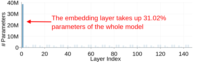
Figure 1: The number of parameters of the layers in GPT-2.

To this end, we propose to compress the embedding layer of LLMs through Tensor-Train Decomposition (TTD) [8] in order to store large embeddings in a low-rank tensor format, with much fewer parameters. This low-rank tensor format is also called TT-format or Matrix Product State (MPS) [9]. Given the fact that in many applications the token vocabulary is ever-changing, we consider each individual token embedding (i.e. each row of the token embedding matrix) rather than taking the token embedding matrix as a whole. Benefiting from the super-compression properties of Tensor Networks (TNs), we tensorize and decompose each token embedding, and then construct a highly efficient format of embedding that can be computed efficiently through distributed computing.

The proposed approach is evaluated on the GPT-2 model. The experiment results show that, using our approach, the embedding layers can indeed be compressed with a compression rate of up to 38.40 times, and with a compression rate of 3.31 didn’t sacrifice model performance. As, due to the approximations involved, for the model performance change after compression, we considered the performance of our TensorGPT on the text reconstruction task, a basic text generation task where the GPT series models excel. We found that with the reconstructed embedding layer from the stored MPS, the overall performance of the GPT-2 even improved under certain TT rank settings, this is likely due to the over-parameterization of the original model.

Our contributions are summarized as follows:

• To our best knowledge, we are the first to utilize the Tensor-Train Decomposition (TTD) and Matrix Product State (MPS) to compress GPT series models.

• A novel approach that treats each token embedding as a Matrix Product State is proposed, which is shown to be very flexible when the token embeddings are inserted or deleted, and also has the potential to be computed in a distributed manner.

• A set of rigorous evaluation metrics is adopted to evaluate our approach. The experimental results show that our compression approach has satisfactory performance, while reducing the number of parameters by a factor of 2.31.

2 Related Work

Among the recent research on the compression of the embedding layers within LLMs tensor with decompositions, the closest to our approach is the work by [13], applied TTD to the embedding layer to reduce the space complexity of large language models. This was achieved by reshaping the embedding matrix into an order-$2N$ tensor which was then decomposed and stored as a Matrix Product Operator. While this approach reduced the number of parameters significantly, the decomposition procedure had to be repeated on the entire embedding matrix every time a new token is added to the dictionary. To solve this issue, instead of decomposing and storing the embedding matrix directly, we propose an approach that decomposes and stores each row of the embedding matrix separately. This reduces the computation costs significantly, as the decomposition can be performed locally on every new token.

Recent progress also includes the compression of the embedding table of a recommendation system in the work by [5], where the tensorized neural network is trained from scratch, yet our proposed approach operates on a pre-trained neural network without an extra training process. In another work [4], Block-Wise Low-Rank Approximation is used to compress very large scale ($\sim$800k vocabulary) embeddings, where the embedding matrices are split into blocks according to the tokens, and then each block is decomposed by SVD. Except for the difference in decomposition methods with our proposed approach, deciding how to reasonably bind certain tokens into blocks for a specific vocabulary requires additional effort.

3 Preliminaries

This section gives brief mathematical preliminaries of tensor algebra, and basic knowledge in LLMs to facilitate the understanding of our proposed methodology in Section 4.

3.1 Tensor and Tensor Operations

Order-N Tensor.

An order-$N$ real-valued tensor is a multi-dimensional array, denoted by a calligraphic font, e.g., $\mathcalbf{A}\in\mathbb{R}^{I_{1}\times\dots\times I_{N}}$, where $N$ is the order of the tensor (i.e., number of modes), and $I_{n}$ ($1\leq n\leq N$) is the size (i.e., the dimension) of its $n$-th mode. Matrices (denoted by bold capital letters, e.g., $\mathbf{A}\in\mathbb{R}^{I_{1}\times I_{2}}$) can be seen as order-$2$ tensors ($N=2$), vectors (denoted by bold lower-case letters, e.g., $\mathbf{a}\in\mathbb{R}^{I}$) can be seen as order-1 tensors ($N=1$), and scalars (denoted by lower-case letters, e.g., $a\in\mathbb{R}$) are order-$0$ tensors ($N=0$).

Tensor Entries.

The $(i_{1},\ldots,i_{N})$-th entry of an order-$N$ tensor is denoted by $a_{i_{1},\cdots,i_{N}}\in\mathbb{R}$, where $i_{n}=1,\ldots,I_{n}$ for $n=1,\ldots,N$. A tensor fiber is a vector of tensor entries obtained by fixing all but one index of the original tensor (e.g., $\mathbf{a}_{:,i_{2},i_{3},\ldots,i_{N}}\in\mathbb{R}^{I_{1}}$). Similarly, a tensor slice is a matrix of tensor entries obtained by fixing all but two indices of the original tensor (e.g., $\mathbf{A}_{:,:,i_{3},i_{4},\ldots,i_{N}}\in\mathbb{R}^{I_{1}\times I_{2}}$).

Tensorization.

A vector, $\mathbf{a}\in\mathbb{R}^{I_{1}I_{2}\cdots I_{N}}$, can be tensorized (or folded) into an order-$N$ tensor, $\mathcalbf{A}\in\mathbb{R}^{I_{1}\times I_{2}\times\cdots\times I_{N}}$, with the relation between their entries defined by

$$\mathcalbf{A}[i_{1},i_{2},\dots,i_{N}]=a_{i}$$ (1)

for all $1\leq i_{n}\leq I_{n}$, where $i=1+\sum_{n=1}^{N}(i_{n}-1)\prod_{k=1}^{n-1}I_{k}$.

Matricization (Mode-n unfolding).

Mode-$n$ matricization of a tensor, $\operatorname{\textit{mat}}\left(\mathcalbf{A},n\right)=\mathbf{A}_{\{n\}}\in\mathbb{R}^{I_{n}\times(I_{1}\cdots I_{n-1}I_{n+1}\cdots I_{N})}$, is a procedure of mapping the elements from a multidimensional array to a two-dimensional array (matrix). Conventionally, such procedure is associated with stacking mode-$n$ fibers (modal vectors) as column vectors of the resulting matrix. For instance, the mode-$1$ unfolding of $\mathcalbf{A}\in\mathbb{R}^{I_{1}\times I_{2}\times\cdots\times I_{N}}$ is represented as $\operatorname{\textit{mat}}\left(\mathcalbf{A},1\right)=\mathbf{A}_{\{1\}}\in\mathbb{R}^{I_{1}\times(I_{2}\cdots I_{N})}$, where the subscript, $\{1\}$, denotes the mode of matricization, and is given by

$$\mathbf{A}_{(1)}\bigg{[}i_{1},\overline{i_{2}i_{3}\ldots i_{N}}\bigg{]}=\mathcalbf{A}[i_{1},i_{2},\ldots,i_{N}]$$ (2)

Note that the overlined subscripts refer to to linear indexing (or Little-Endian) [10], given by:

$$\overline{i_{1}i_{2}\dots i_{N}} =1+\sum_{n=1}^{N}\Bigg{[}(i_{n}-1)\prod_{n^{\prime}=1}^{n-1}I_{n^{\prime}}\Bigg{]}$$ (3)

$$=1+i_{1}+(i_{2}-1)I_{1}+\cdots+(i_{n}-1)I_{1}\ldots I_{N-1}$$

Vectorization.

Given an order-$N$ tensor, $\mathcalbf{A}\in\mathbb{R}^{I_{1}\times\cdots\times I_{N}}$, its vectorization reshapes the multidimensional array into a large vector, $\operatorname{\textit{vec}}\left(\mathcalbf{A}\right)=\mathbf{\bar{a}}\in\mathbb{R}^{I_{1}\cdots I_{N}}$.

Tensor contraction.

The contraction of an order-$N$ tensor, $\mathcalbf{A}\in\mathbb{R}^{I_{1}\times\dots\times I_{N}}$, and an order-$M$ tensor $\mathcalbf{B}\in\mathbb{R}^{J_{1}\times\dots\times J_{M}}$, over the $n$^th and $m$^th modes respectively, where $I_{n}=J_{m}$, results in $\mathcalbf{C}\in\mathbb{R}^{I_{1}\times\cdots\times I_{n-1}\times I_{n+1}\times\cdots\times I_{N}\times J_{1}\times\cdots\times J_{m-1}\times J_{m+1}\times J_{M}}$, with entries

$$c_{i_{1},\dots,i_{n-1},i_{n+1},\dots,i_{N},j_{1},\dots,j_{m-1},j_{m+1},\dots,j_{M}}=\sum_{i_{n}=1}^{I_{n}}a_{i_{1},\dots,i_{n-1},i_{n},i_{n+1},\dots,i_{N}}b_{j_{1},\dots,j_{m-1},i_{n},j_{m+1},\dots,j_{M}}$$ (4)

A $(2,1)$-tensor contraction between two order-$2$ tensors, $\textbf{A}\in\mathbb{R}^{I_{1}\times I_{2}}$ and $\textbf{B}\in\mathbb{R}^{J_{1}\times J_{2}}$, where $I_{2}=J_{1}$, is equivalent to a standard matrix multiplication, $\textbf{C}=\textbf{A}\times_{2}^{1}\textbf{B}=\textbf{A}\textbf{B}\in\mathbb{R}^{I_{1}\times J_{2}}$. Similarly, a $(2,1)$-tensor contraction between an order-$2$ tensor, $\textbf{A}\in\mathbb{R}^{I_{1}\times I_{2}}$, and an order-$1$ tensor, $\textbf{b}\in\mathbb{R}^{J_{1}}$, where $I_{2}=J_{1}$, is equivalent to a standard matrix-by-vector multiplication, $\textbf{c}=\textbf{A}\times_{2}^{1}\textbf{b}=\textbf{A}\textbf{b}\in\mathbb{R}^{I_{1}}$.

3.2 Token, Token Embeddings and Embedding Layer in LLMs

Token and Tokenization.

In natural language processing (NLP), a token is a meaningful unit of text, such as a word, punctuation mark, or other element that contributes to the structure and meaning of a sentence or document. Tokens are produced through a process known as tokenization, which involves breaking down a piece of text into individual units. The GPT series models employ a widely used tokenization method named Byte Pair Encoding (BPE) [7]. The BPE breaks down text into varying-length subword units, and is particularly useful for languages with complex morphology or when dealing with out-of-vocabulary words.

Token Embedding and Embedding Layer in LLMs.

In the context of LLMs, “embedding” refers to converting discrete input tokens into continuous vector representations. These representations are commonly known as word embeddings or token embeddings. In LLMs, the embedding layer is responsible for output token embeddings according to the sequential input tokens. This layer maps each input token to a high-dimensional vector that captures the semantic and syntactic information about the meaning and context of a token. Normally, an embedding layer considers a set of tokens $\{v\}$ of size $V$ (also known as “vocabulary”), where $v$ represents a considered token. For each token $v$, a token embedding $\textbf{x}_{v}$ of dimension $D$ is assigned by the embedding layer, that is, $\textbf{x}_{v}\in\mathbb{R}^{D}$. The weights of the embedding layer are represented as an embedding weight matrix W, where $\textbf{W}\in\mathbb{R}^{V\times D}$. In practice, if the token embedding dimension $D$ is excessively large, there would be excessive parameter complexity, resulting in high storage costs for the embedding layer, and thereafter high storage costs for the whole language model.

Remark 1.

The embedding weight matrix W can be seen as a lookup table. A basic embedding generation finds the token embeddings corresponding to all the input tokens and stacks them according to the input order. It should be noted that in the current LLMs, such as GPT-like and BERT-like models, the position and mask information of the tokens are also encoded into the embeddings. In these cases, a token embedding $\textbf{x}_{v}$ is not merely generated via a lookup process.

4 Methodology

This section gives a brief introduction to the technical cornerstones that our approach relies on, and a detailed description of our proposed approach.

4.1 Tensor-Train Decomposition (TTD) and Matrix Product State (MPS)

Tensor-Train Decomposition [14, 8] was introduced to help mitigate the computational bottlenecks that arise from the curse of dimensionality, as tensor algorithms can become intractable for high-order tensors. The most common form of TT is the Matrix Product State (MPS or TT-MPS), introduced in the quantum physics community [11], which applies the Tensor-Train Singular Value Decomposition (TT-SVD) algorithm described in Algorithm 1 [12] to decomposes a large order-$N$ tensor, $\mathcalbf{X}\in\mathbb{R}^{I_{1}\times I_{2}\times\cdots\times I_{N}}$, into $N$ smaller $2$-nd or $3$-rd order core tensors, $\mathcalbf{G}^{(n)}\in\mathbb{R}^{R_{n-1}\times I_{n}\times R_{n}}$ for $n=1,\dots,N$, such that

$$\mathcalbf{X}\approx\mathcalbf{G}^{(1)}\times_{2}^{1}\mathcalbf{G}^{(2)}\times_{3}^{1}\mathcalbf{G}^{(3)}\times_{3}^{1}\cdots\times_{3}^{1}\mathcalbf{G}^{(N)}$$ (5)

The tensors $\mathcalbf{G}^{(1)},\ldots,\mathcalbf{G}^{(N)}$ are referred to as the core tensors, while the set $\{R_{0},\dots,R_{N}\}$, where $R_{0}=R_{N}=1$, represents the TT-rank of the TT decomposition. By defining $\mathcalbf{G}^{(n)}_{:,i_{n},:}$, $i_{n}=1,\dots,I_{N}$ as the $i_{n}$-th horizontal slice of tensor $\mathcalbf{G}^{(n)}$, the MPS assumes the element-wise form as

$$x_{i_{1},i_{2},\dots,i_{N}}=\mathbf{G}^{(1)}_{:,i_{1},:}\cdots\mathbf{G}^{(N)}_{:,i_{N},:}$$ (6)

Input :  Data tensor, $\mathcalbf{X}\in\mathbb{R}^{I_{1}\times I_{2}\times\cdots\times I_{N}}$, and approximation accuracy, $\epsilon$

Output :  Core tensors, $\mathcalbf{G}^{(1)},\dots,\mathcalbf{G}^{(N)}$, approximating $\mathcalbf{X}\in\mathbb{R}^{I_{1}\times I_{2}\times\cdots\times I_{N}}$

Initialize cores, $\mathcalbf{G}^{(1)},\dots,\mathcalbf{G}^{(N)}$, and $R_{0}=1$

Compute truncation parameter $\delta=\frac{\epsilon}{\sqrt{N-1}}||\mathcalbf{X}||_{F}$

$\mathcalbf{Z}\leftarrow\mathcalbf{X}$, and $\mathbf{Z}\leftarrow\mathbf{Z}_{(1)}$

for $n=1$ to $N-1$ do

       Compute $\delta$-truncated SVD: $\mathbf{Z}=\mathbf{USV}+\mathbf{E},\text{ s.t. }{||\mathbf{E}||_{F}}\leq\delta;\mathbf{U}\in\mathbb{R}^{R_{(n-1)}I_{n}\times R_{n}}$

      $\mathcalbf{G}^{(n)}\leftarrow$ reshape $\left(\mathbf{U},[R_{(n-1)},I_{n},R_{n}]\right)$

      $\mathbf{Z}\leftarrow$ reshape $\left(\mathbf{SV}^{T},[R_{n}I_{(n+1)},I_{(n+2)}I_{(n+3)}\dots I_{N}])\right)$

$\mathcalbf{G}^{(N)}\leftarrow\mathbf{Z}$

return $\mathcalbf{G}^{(1)},\mathcalbf{G}^{(2)},\dots,\mathcalbf{G}^{(N)}$

Algorithm 1 Tensor-Train Singular Value Decomposition (TT-SVD)

4.2 MPS formatted Token Embedding

As mentioned in Section 1 and Section 2, when the vocabulary changes, the tensor decomposition should be re-executed from scratch if the decomposition object is the whole embedding weight matrix. On the other hand, loading the whole embedding weight matrix into the memory and then decomposing also requires massive memory and computation resources. Using the notions in Section 3 and Algorithm 1, decomposing a 2-order W requires roughly the computation cost of $\mathcal{O}(VD^{2})$.

Rather than decomposing the whole embedding weight matrix, we propose to decompose each token embedding. In this way, each token embedding is reshaped into an order-$N$ tensor, $\texttt{ten}\left(\textbf{x}_{v}\right)=\mathcalbf{X}\in\mathbb{R}^{I_{1}\times\cdots\times I_{N}}$ such that $D=\prod_{k=1}^{N}I_{k}$, which is then decomposed and stored in Matrix Product State (MPS) form as $\mathcalbf{X}\approx\mathcalbf{G}^{(1)}\times_{3}^{1}\cdots\times_{3}^{1}\mathcalbf{G}^{(N)}$. In other words, instead of storing the entire token embedding $\textbf{x}\in\mathbb{R}^{D}$, we store the corresponding MPS cores, $\mathcalbf{G}^{(n)}\in\mathbb{R}^{R_{n-1}\times I_{n}\times R_{n}}$, for $n=1,\ldots,N$.

This approach has two advantages:

1. Lower storage cost: The space complexity reduces from an original $\mathcal{O}\left(I^{N}\right)$ (exponential in $N$) to $\mathcal{O}\left(NR^{2}I\right)$ (linear in $N$), where $R_{n}=R$ and $I_{n}=I$ for all $n=1,\ldots,N$ for simplicity;

2. Affordable computation cost of TTD on resource-constrained nodes. Since token embeddings are decomposed individually, the decomposition of an individual token embedding or a small number of token embeddings can be offloaded to a single resource-constrained node (thread, process or device). On a single node, the computation cost is reduced from $\mathcal{O}(VD^{2})$ to $\mathcal{O}(D)$. Also considering the ever-changing vocabulary, this approach has the potential to be deployed in a dynamic distributed system.

Remark 2.

The considered tensor embedding procedure is highly effective for a small rank tensor, $R$, small MPS dimension, $I$, and large tensor order $N$. In practice, the original vector embedding dimension can be chosen to be a power of $2$ in order to maximize the compression as $D=I^{N}=2^{N}$.

Remark 3.

In practice, the MPS is a low-rank approximation of the original embedding. However, the approximation error will tend to zero as the rank $R$ increases. Therefore, the choice of the rank $R$ will have to balance the trade-off between the compression power and the approximation ability.

Remark 4.

Without considering the position and mask information mentioned in Remark 1, the MPS token embedding approach can be directly used to accelerate the token embedding mapping and compress the stored embeddings. However, since the language models we discuss in this paper are typical LLMs containing position and mask encoding, we shall not consider the above two.

5 Experiment

Table 1: Compression rate $\eta$ of the embedding layer, distortion error (MAE or norm-MAE) and the compatibility (Generation Loss) of the reconstructed embedding layer. All the results were implemented with the Tensor-Train Decomposition on the GPT-2 model and GLUE/MRPC dataset. For the text reconstruction task, the generation loss of the original model is 13.71, and regarding this, any setting where the generation loss is lower than 13.71 has better text generation performance than the original model. Decomposing embedding weight matrix W directly with two cores achieves a higher compression rate than our approach; without a decline of generation loss, the compression rate can be up to 23.64$\times$. However, our approach has advantages mentioned in Section 4.2, and achieves the best text reconstruction performance with the lowest generation loss of 9.01 among all the settings, when the compression rate is 3.31$\times$.

Methods	TT cores’ ranks	Compression Rate $\eta$	MAE of Layer Reconstruction	Embeddings norm-MAE ($\times 10^{-3}$)	Generation Loss
Original	—-				13.71
TTD weight matrix with 2 cores (SVD)	1,2,1	378.22$\times$	0.1209	2.115	20.17
	1,4,1	189.11$\times$	0.1079	2.260	22.00
	1,8,1	94.56$\times$	0.1014	2.401	16.70
	1,16,1	47.28$\times$	0.0989	2.481	14.70
	1,32,1	23.64$\times$	0.0917	2.311	10.14
	1,641,1	11.82$\times$	0.0848	2.113	10.13
	1,128,1	5.91$\times$	0.0794	1.848	10.65
	1,256,1	2.95$\times$	0.0690	1.500	12.74
	1,512,1	1.48$\times$	0.0458	1.012	9.82
TTD for each token $\texttt{ten}(\textbf{x}_{v})$	1,1,1,1,1,1,1,1,1,1,1	38.40$\times$	0.1120	2.573	20.77
	1,1,1,1,1,2,1,1,1,1,1	32.00$\times$	0.1119	3.063	20.88
	1,1,1,1,2,2,2,1,1,1,1	21.33$\times$	0.1115	2.957	27.81
	1,1,1,1,2,4,2,1,1,1,1	14.77$\times$	0.1113	2.864	28.60
	1,2,2,2,2,2,2,2,2,2,1	10.67$\times$	0.1090	2.695	19.40
	1,1,2,4,4,4,4,4,4,1,1	4.00$\times$	0.1054	2.628	22.63
	1,2,4,4,4,4,4,4,4,2,1	3.31$\times$	0.0995	2.574	9.01
	1,2,2,4,8,8,8,4,2,2,1	2.33$\times$	0.0965	2.549	51.24
	1,2,4,8,8,8,8,8,4,2,1	1.13$\times$	0.0744	0.883	39.88

5.1 Dataset, Tokenization and Language Model

The text dataset used for the experiments was a mixed version of General Language Understanding Evaluation (GLUE) [1] and Microsoft Research Paraphrase Corpus (MRPC) [3], with 11,602 English sentences in total. For the tokenization, we chose the BPE mentioned in Section 3.2, since it is popular in GPT series models. The language model we used was the HuggingFace version of GPT-2, with an embedding weight matrix $\textbf{W}\in\mathbb{R}^{50257\times 768}$, where the vocabulary size $V$ is 50,257 and the token embedding dimension $D$ is 768.

5.2 Implementation

The 2.12.0 version of TensorFlow was used for the GPT-2 model, while Tensorly [6], a Python package for tensor learning, was used to decompose the token embeddings and the embedding layer.

According to Remark 2 and also to take advantage of the hierarchical structure and multiway interactions expressiveness of Tensor-Train Decomposition, we reshaped each token embedding $\textbf{x}_{v}$ into a power of 2 format for tensorization, that is, $\texttt{ten2}\left(\textbf{x}_{v}\right)=\mathcalbf{X}\in\mathbb{R}^{2\times 2\times\cdots\times 2}$. The current token embedding dimension $D$ is 768, which cannot be factored into a power of 2. Therefore, we padded each token embedding with zeros to reach a length of 1024, which is the nearest power of 2 to 768 and is a feasible dimension for $\texttt{ten2}(\cdot)$. Note that when Tensor-Train Decomposition is applied to decompose $\textbf{x}_{v}$, and then to reconstruct $\textbf{x}_{v}$ back, the values of each token embedding $\textbf{x}_{v}$ from index 768 to 1,024 are almost zeros.

5.3 Evaluation Metrics

Compression Rate.

We used the embedding layer compression ratio to describe the degree of size reduction and efficiency in embedding layer storage. More mathematically, the compression rate $\eta$ is the ratio of the original embedding layer size to the sum of the size of the compressed token.

$$\eta=\frac{V\times D}{\sum_{j=1}^{V}\sum_{k=1}^{N}|\mathcalbf{G}^{(k)}_{j}|}$$ (7)

where $\mathcalbf{G}^{(k)}_{j}$ denotes the $k$th tensor core of the $j$th token after decomposing each token embedding $\textbf{x}_{j}$ in the embedding layer weight matrix W.

Distortion Error.

The distortion metrics were used to describe the compression fidelity, that is, the similarity between the original embedding layer weights and reconstructed embedding layer weights, or the original reconstructed token embeddings and reconstructed token embeddings. Considering the inference process of the embedding layer, the distortion metrics were first calculated sentence by sentence and then derived from the average. There are two kinds of distortion measurements of the embedding weight matrix and token embeddings:

• Mean absolute error (MAE) for the embedding weight matrix reconstruction: We used MAE to measure the difference between the original embedding layer weight matrix and the reconstructed embedding layer weight matrix. A lower MAE suggests that the compressed embedding layer weights closely resemble the original embedding layer weights, indicating a higher level of fidelity in the compression process.

• Normalized mean absolute error (norm-MAE) for the token embeddings: The token embedding values vary from minus several hundred to several hundred, and to align them for easier comparison like embedding weight matrix, we used the normalized mean absolute error. The norm-MAE is the ratio of mean absolute error and the difference between the maximum and minimum values of original embeddings. Similar to MAE for the embedding weight matrix, a lower norm-MAE indicates a higher compression fidelity.

Compatibility with the subsequent GPT-2 network blocks.

The primary function of GPT-like models is natural language generation. We here conducted a text reconstruction task to verify if the reconstructed embedding layer can collaborate effectively with the subsequent GPT-2 network blocks for natural language generation. The purpose of this task was to reconstruct the original input data from the encoded representation in the embedding layer and the subsequent network blocks, similar to an autoencoder. This part serves as a sanity check for the stored information in the reconstructed embedding layer, and causes evaluation via text generation loss of the GPT-2 model.

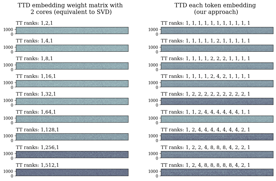
Figure 2: Visualization of the reconstruction distortion error (MAE) for the GPT-2 embedding weight matrix W. In each heatmap, a point with location index $(j,p)$ with lighter colors than other points indicates a more accurate reconstruction at this point than the other points, while with darker colour means less accurate reconstruction, where $j=1,\ldots,V$ and $p=1,\ldots,D$ . For better visualization, we reshaped W from the shape of $50257\times 768$ to $25128\times 1536$, with a sacrifice of one token embedding to enable reshaping.

5.4 Experiment Results

All the evaluation metrics described in Section 5.3 on the dataset GLUE/MRPC are shown in Table 1. There are two approaches tested for a comprehensive analysis - our proposed approach introduced in Section 4, and the approach of directly decomposing the embedding weight matrix W into two TT cores. The latter is actually equivalent to performing tensor SVD.

As the ranks of TT cores increase, both approaches exhibit a decrease in compression rate, fidelity of embedding layer reconstruction (MAE), and fidelity of reproduced token embeddings (norm-MAE). There is no apparent decline or increase in the text generation loss, possibly because this metric is highly dependent on the dataset itself. In all settings, the lowest text generation loss was 9.01, which was achieved by our approach when the TT ranks were 1,2,4,4,4,4,4,4,1,1.

5.5 Discussion

We visualized the MAE for the reconstruction of embedding weight matrix W in Figure 2. For better visualization, we folded the dimension that represents the vocabulary index into a reasonable matrix shape. In Figure 2, the lighter colour indicates a lower MAE, and the darker colour indicates a higher MAE.

From the visualization, since the change of colour shading is not stable, it can be inferred that the decrease in compression fidelity does not decrease smoothly as the TT ranks increase, even for SVD. As for the decomposition of each token embedding, we can identify specific areas where the light (lower MAE) lines consistently appear, suggesting that some dimensions of the token embeddings are more precise in reconstruction. These dimensions may have the potential for further compression.

6 Conclusion and Future Work

In the context of Large Language Models (LLMs), this study has suggested a compression approach for the embedding layer. The approach has constructed a power-2 tensor Matrix Product State (MPS) format for each token embedding in the embedding weight matrix, followed by the further application of the Tensor-Train Decomposition (TTD). This approach has demonstrated the advantages of adaptability to the ever-changing vocabulary and in a distributed manner, together with the compression of GPT-2 and has achieved a 3.31$\times$ compression rate with an improved model performance in the text reconstruction task.

The superiority of Matrix Product State has not been not fully explored in our current implementation. An unsolved problem is the integration of MPS into the computation process of token embeddings within other encoded information (e.g. position or mask encodings) in LLMs, so that the LLMs can run faster, and be able to be deployed on lower-end devices. Furthermore, if the generated token embeddings are also formatted by MPS, the embedding generation process might be lighter and easier to store as well.

References

- [1] Wang, A., Singh, A., Michael, J., Hill, F., Levy, O. & Bowman, S. GLUE: A Multi-Task Benchmark and Analysis Platform for Natural Language Understanding. Proceedings Of The 2018 EMNLP Workshop BlackboxNLP: Analyzing And Interpreting Neural Networks For NLP. pp. 353-355 (2018)
- [2] Radford, A., Wu, J., Child, R., Luan, D., Amodei, D. & Sutskever, I. Language models are unsupervised multitask learners. OpenAI Blog. 1, 9 (2019)
- [3] Dolan, B. & Brockett, C. Automatically Constructing a Corpus of Sentential Paraphrases. Proceedings Of The Third International Workshop On Paraphrasing. (2005)
- [4] Chen, P., Si, S., Li, Y., Chelba, C. & Hsieh, C. Groupreduce: Block-wise low-rank approximation for neural language model shrinking. Advances In Neural Information Processing Systems. 31 (2018)
- [5] Yin, C., Acun, B., Wu, C. & Liu, X. Tt-rec: Tensor train compression for deep learning recommendation models. Proceedings Of Machine Learning And Systems. 3 pp. 448-462 (2021)
- [6] Kossaifi, J., Panagakis, Y., Anandkumar, A. & Pantic, M. TensorLy: Tensor Learning in Python. Journal Of Machine Learning Research. 20, 1-6 (2019), http://jmlr.org/papers/v20/18-277.html
- [7] Gage, P. A new algorithm for data compression. C Users Journal. 12, 23-38 (1994)
- [8] Oseledets, I. Tensor-train decomposition. SIAM Journal On Scientific Computing. 33, 2295-2317 (2011)
- [9] Perez-Garcia, D., Verstraete, F., Wolf, M. & Cirac, J. Matrix product state representations. ArXiv Preprint Quant-ph/0608197. (2006)
- [10] Dolgov, S. & Savostyanov, D. Alternating minimal energy methods for linear systems in higher dimensions. SIAM Journal On Scientific Computing. 36, A2248-A2271 (2014)
- [11] Cichocki, A. Era of Big Data Processing: A New Approach via Tensor Networks and Tensor Decompositions. Proceedings Of The International Workshop On Smart Info-Media Systems In Asia. (2014,3)
- [12] Cichocki, A., Lee, N., Oseledets, I., Phan, A., Zhao, Q. & Mandic, D. Tensor networks for dimensionality reduction and large-scale optimization: Part 1: low-rank tensor decompositions. Foundations And Trends In Machine Learning. 9, 249-429 (2016)
- [13] Khrulkov, V., Hrinchuk, O., Mirvakhabova, L. & Oseledets, I. Tensorized Embedding Layers. Proceedings Of The 2020 Conference On Empirical Methods In Natural Language Processing: Findings. pp. 4847-4860 (2020)
- [14] Oseledets, I. & Tyrtyshnikov, E. Breaking the curse of dimensionality, or how to use SVD in many dimensions. SIAM Journal On Scientific Computing.31, 3744-3759 (2009)