Some preconditioning techniques for a class of double saddle point problems

Abstract

In this paper, we describe and analyze the spectral properties of a number of exact block preconditioners for a class of double saddle point problems. Among all these, we consider an inexact version of a block triangular preconditioner providing extremely fast convergence of the FGMRES method. We develop a spectral analysis of the preconditioned matrix showing that the complex eigenvalues lie in a circle of center $(1,0)$ and radius 1, while the real eigenvalues are described in terms of the roots of a third order polynomial with real coefficients. Numerical examples are reported to illustrate the efficiency of inexact versions of the proposed preconditioners, and to verify the theoretical bounds.

AMS classification: 65F10, 65F50, 56F08.

Keywords: Double saddle point problems. Preconditioning. Krylov subspace methods.

1 Introduction

This paper is concerned with a number of block preconditioners for the numerical solution of large and sparse linear system of equations of double saddle-point type of the form

$$\mathcal{A}w\equiv\begin{pmatrix}A&B^{T}&0\\ B&0&C^{T}\\ 0&C&0\end{pmatrix}\begin{pmatrix}x\\ y\\ z\end{pmatrix}=\begin{pmatrix}f\\ g\\ h\end{pmatrix}\equiv b,$$ (1.1)

where $A\in\mathbb{R}^{n\times n}$ is a symmetric positive definite matrix, $B\in\mathbb{R}^{m\times n}$ and $C\in\mathbb{R}^{l\times m}$ have full row rank, $f\in\mathbb{R}^{n}$, $g\in\mathbb{R}^{m}$ and $h\in\mathbb{R}^{l}$ are given vectors. Such linear systems arise in a number of scientific applications including constrained least squares problems [1], constrained quadratic programming [2], magma-mantle dynamics [3], to mention a few; see, e.g. [4, 5, 6]. Similar block structures arise e.g. in liquid crystal director modeling or in the coupled Stokes-Darcy problem, and the preconditioning of such linear systems has been considered in [7, 8, 9, 10].

Obviously, the matrix of system (1.1) is symmetric and can be considered as a $2\times 2$ block matrix [11]. Due to the fact that these saddle point matrices are typically large and sparse, their iterative solution is recommended e.g. by Krylov subspace iterative methods [13]. In order to improve the efficiency of iterative methods, some preconditioning techniques are employed.

To solve iteratively the linear system (1.1), a number of preconditioning methods have been investigated and studied in the literature. In [14], Huang developed the block diagonal preconditioner $\mathcal{P}_{D}$ and its inexact version $\widehat{\mathcal{P}}_{D}$ which are of the forms

$$\mathcal{P}_{D}=\begin{pmatrix}A&0&0\\ 0&S&0\\ 0&0&X\end{pmatrix},\qquad\widehat{\mathcal{P}}_{D}=\begin{pmatrix}\widehat{A}&0&0\\ 0&\widehat{S}&0\\ 0&0&\widehat{X}\end{pmatrix},$$ (1.2)

where $S=BA^{-1}B^{T},\ X=CS^{-1}C^{T}$ and $\widehat{A},\widehat{S}$ and $\widehat{X}$ are symmetric positive definite approximations of $A,S$, and $X$, respectively. Exact and inexact versions of the block diagonal preconditioner $\widehat{\mathcal{P}}_{D}$ have been analyzed in [12]. Cao [11] considered the equivalent linear system

$$\mathcal{A}w\equiv\begin{pmatrix}A&B^{T}&0\\ -B&0&-C^{T}\\ 0&C&0\end{pmatrix}\begin{pmatrix}x\\ y\\ z\end{pmatrix}=\begin{pmatrix}f\\ -g\\ h\end{pmatrix}\equiv b,$$ (1.3)

and proposed the shift-splitting iteration of the form

$$\frac{1}{2}(\alpha I+\mathcal{A})w^{(k+1)}=\frac{1}{2}(\alpha I-\mathcal{A})w^{(k)}+b,$$ (1.4)

which leads to the preconditioner

$$\mathcal{P}_{SS}=\frac{1}{2}\begin{pmatrix}\alpha I+A&B^{T}&0\\ -B&\alpha I&-C^{T}\\ 0&C&\alpha I\end{pmatrix},$$ (1.5)

where $\alpha$ is a positive constant and $I$ is the identity matrix of appropriate size. In addition, a relaxed version of the shift-splitting preconditioner has been considered by dropping the shift parameter in the (1,1) block of $\mathcal{P}_{SS}$. In [15] two block preconditioners are proposed, and the spectral distributions of their inexact versions are described.

In [16], three exact block preconditioners for solving (1.1) have been introduced and analyzed which are defined as

$$\mathcal{P}_{1}=\begin{pmatrix}A&0&0\\ B&-S&C^{T}\\ 0&0&-X\end{pmatrix},\quad\mathcal{P}_{2}=\begin{pmatrix}A&0&0\\ B&-S&C^{T}\\ 0&0&X\end{pmatrix},\quad\mathcal{P}_{3}=\begin{pmatrix}A&B^{T}&0\\ B&-S&0\\ 0&0&-X\end{pmatrix}.$$ (1.6)

Moreover, it is shown that the preconditioned matrices corresponding to the above preconditioners only have at most three distinct eigenvalues. More recently, Wang and Li [17] have proposed an exact and inexact parameterized block symmetric positive definite preconditioner for solving the double saddle point problem (1.1).

Enlightened by the type $\mathcal{P}$ preconditioners in (1.6), we describe several other block preconditioning approaches to be employed within a Krylov subspace methods for the solution of linear system of equations (1.1),

$$\mathcal{Q}_{1}=\begin{pmatrix}A&B^{T}&0\\ 0&-S&0\\ 0&0&X\end{pmatrix},\quad\mathcal{Q}_{2}=\begin{pmatrix}A&B^{T}&0\\ 0&S&C^{T}\\ 0&0&-X\end{pmatrix},\quad\mathcal{Q}_{3}=\begin{pmatrix}A&B^{T}&0\\ 0&-S&C^{T}\\ 0&0&\pm X\end{pmatrix},$$ (1.7)

and the block preconditioners of the forms

$$\mathcal{Q}_{4}=\begin{pmatrix}A&B^{T}&0\\ B&0&0\\ 0&C&\pm X\end{pmatrix},\quad\mathcal{Q}_{5}=\begin{pmatrix}A&B^{T}&0\\ B&0&0\\ 0&0&X\end{pmatrix}.$$ (1.8)

We analyze the spectral distribution of the corresponding preconditioned matrices which in all cases have at most three distinct eigenvalues thus guaranteeing the finite termination of e.g. the GMRES iterative method. In realistic problems the proposed preconditioners can not be used exactly since they require (for their application)

1. Solution of a system with $A$,
   

2. Explicit computation of $S=BA^{-1}B^{T}$,
   

3. Solution of a system with $S$,
   

4. Explicit computation of $X=CS^{-1}C^{T}$,
   

5. Solution of a system with $X$.

Particularly, steps 2. and 4. require inversion of the (possibly sparse) matrices $A$ and $S$. Practical application of the described preconditioners is then subjected to approximation of matrices $A,S$ and $X$ with $\widehat{A},\widehat{S}$ and $\widehat{X}$, respectively.

To measure the effects of such approximation on the spectral properties of the preconditioned matrix we considered the block triangular preconditioner $\mathcal{Q}_{3}$ (with the plus sign in (3,3) block), and give bound on the complex and real eigenvalues in terms of the (real and positive) eigenvalues of $\widehat{A}^{-1}A$, $\widehat{S}^{-1}S$, $\widehat{X}^{-1}X$.

The outline of this work is described as follows. In section 2, we derive and analyze some exact block preconditioners for solving double saddle point problem (1.1). In section 3, we test the inexact versions of the proposed preconditioners on a test case in combination with the FGMRES iterative method. We then focus in section 4 on the spectral analysis of the block preconditioner which revealed the most efficient. Bound on truly complex as well as on real eigenvalues are developed for this preconditioner and compared with the actual spectral distribution. Some further results about the real eigenvalues of a simplified version of the triangular preconditioner are developed and tested in section 5. Finally, we state some conclusions in section 6.

2 Block preconditioners and eigenvalue analysis

Let us consider the preconditioners in (1.7) and (1.8). We observe that these preconditioners are nonsingular since $A$ is symmetric positive definite and both $B$ and $C$ have full row rank. We know that the eigenvalues of $\mathcal{A}\mathcal{Q}^{-1}$ and $\mathcal{Q}^{-1}\mathcal{A}$ (for general preconditioner $\mathcal{Q}$) are equal, so that spectral results can be given in terms of any of the two matrices. In the following the eigenvalues of the preconditioned matrices corresponding to the proposed preconditioners are determined. The notations $\sigma(.)$ and $||.||$ denote the set of all eigenvalues of a matrix and the Euclidean norm of a vector, respectively. We use $\Re(\lambda)$ and $\Im(\lambda)$ to denote the real and imaginary parts of a complex eigenvalue $\lambda$. The preconditioners $\mathcal{Q}_{3}$ and $\mathcal{Q}_{4}$ with positive (3,3)-block are denoted by $Q_{3,+}$ and $Q_{4,+}$.

Theorem 1.

Suppose that $A\in\mathbb{R}^{n\times n}$ is symmetric positive definite and $B\in\mathbb{R}^{m\times n}$ and $C\in\mathbb{R}^{l\times m}$ are matrices with full row rank. Then the preconditioner $\mathcal{Q}_{1}$ for $\mathcal{A}$ satisfies

$$\sigma(\mathcal{A}\mathcal{Q}_{1}^{-1})\in\Big{\{}1,\frac{1}{2}(1\pm\sqrt{3}i)\Big{\}}.$$

Proof.

First we must compute $\mathcal{Q}_{1}^{-1}$. An easy calculations yields that

$$\mathcal{Q}_{1}^{-1}=\begin{pmatrix}A^{-1}&A^{-1}B^{T}S^{-1}&0\\ 0&-S^{-1}&0\\ 0&0&X^{-1}\end{pmatrix},$$ (2.1)

It follows directly from (2.1) that

$$\mathcal{A}\mathcal{Q}_{1}^{-1}=\begin{pmatrix}I&0&0\\ BA^{-1}&I&C^{T}X^{-1}\\ 0&-CS^{-1}&0\end{pmatrix}.$$ (2.2)

We now determine the eigenvalues of the preconditioned matrix $\mathcal{A}\mathcal{Q}_{1}^{-1}$ by using the Laplace expansion. Therefore, the characteristic polynomial of $\mathcal{A}\mathcal{Q}_{1}^{-1}$ is given by

$$q(\lambda)=\text{det}(\lambda I-\mathcal{A}\mathcal{Q}_{1}^{-1})=(\lambda-1)^{n}\begin{vmatrix}(\lambda-1)I&-C^{T}X^{-1}\\ CS^{-1}&\lambda I\end{vmatrix}.$$ (2.3)

Clearly, $\lambda=1$ is an eigenvalue of $\mathcal{A}\mathcal{Q}_{1}^{-1}$ with algebraic multiplicity at least $n$. To determine the rest of eigenvalues, we seek $\lambda\neq 1,\>x_{2}$ and $x_{3}$ satisfying

$$(\lambda-1)x_{2}-C^{T}X^{-1}x_{3} =0,$$ (2.4)

$$CS^{-1}x_{2}+\lambda x_{3} =0.$$ (2.5)

Computing $x_{2}=\frac{1}{\lambda-1}CS^{-1}x_{3}$ from equation (2.4) and substituting the value $x_{2}$ into equation (2.5), we get

$$\Big{(}\lambda^{2}I-\lambda I+I\Big{)}x_{3}=0$$ (2.6)

Note that the vector $x_{3}$ must be nonzero, otherwise if $x_{3}=0$, then $x_{2}=0$, and we saw that $x_{1}=0$ if $\lambda\neq 1$. Without loss of generality, we can assume that $x_{3}^{*}x_{3}=1$. Multiplying equation (2.6) on the left by $x_{3}^{*}$, we obtain

$$\lambda^{2}-\lambda+1=0.$$ (2.7)

The roots of (2.7) are equal to $\lambda=\frac{1}{2}(1\pm\sqrt{3}i)$, which completes the proof. ∎

Remark 1.

From the foregoing theorem it is evident that the preconditioned matrix $\mathcal{A}\mathcal{Q}_{1}^{-1}$ has eigenvalues clustered around three values 1, $\frac{1}{2}(1+\sqrt{3}i)$, and $\frac{1}{2}(1-\sqrt{3}i)$, therefore one can expect rapid convergence for the preconditioned GMRES method.

Remark 2.

It is easy to verify that the preconditioned matrix $\mathcal{T}=\mathcal{A}\mathcal{Q}_{1}^{-1}$ satisfies the following polynomial

$$(\mathcal{T}-\mathcal{I})(\mathcal{T}^{2}-\mathcal{T}+\mathcal{I})=0.$$

Since the above relation can be factorized into distinct linear factors (over $\mathbb{R}$), we conclude that $\mathcal{T}$ is diagonalizable and has at most three distinct eigenvalues $1,\frac{1}{2}(1\pm\sqrt{3}i)$.

Theorem 2.

Suppose that $A\in\mathbb{R}^{n\times n}$ is symmetric positive definite and $B\in\mathbb{R}^{m\times n}$ and $C\in\mathbb{R}^{l\times m}$ are matrices with full row rank. Then the preconditioner $\mathcal{Q}_{2}$ for $\mathcal{A}$ satisfies

$$\sigma(\mathcal{A}\mathcal{Q}_{2}^{-1})\in\Big{\{}\pm 1,\pm i\Big{\}}.$$

Proof.

Straightforward calculations reveal that

$$\mathcal{Q}_{2}^{-1}=\begin{pmatrix}A^{-1}&-A^{-1}B^{T}S^{-1}&-A^{-1}B^{T}S^{-1}C^{T}X^{-1}\\ 0&S^{-1}&S^{-1}C^{T}X^{-1}\\ 0&0&-X^{-1}\end{pmatrix}.$$ (2.8)

It follows from (2.8) that

$$\mathcal{A}\mathcal{Q}_{2}^{-1}=\begin{pmatrix}I&0&0\\ BA^{-1}&-I&-2C^{T}X^{-1}\\ 0&CS^{-1}&I\end{pmatrix}.$$ (2.9)

To proceed we use the Laplace expansion to determine the eigenvalues of $\mathcal{A}\mathcal{Q}_{2}^{-1}$. Therefore, the characteristic polynomial of $\mathcal{A}\mathcal{Q}_{2}^{-1}$ is given by

$$\widehat{q}(\lambda)=\text{det}(\lambda I-\mathcal{A}\mathcal{Q}_{2}^{-1})=(\lambda-1)^{n}\begin{vmatrix}(\lambda+1)I&2C^{T}X^{-1}\\ -CS^{-1}&(\lambda-1)I\end{vmatrix}.$$ (2.10)

It is clear that $\lambda=1$ is an eigenvalue of $\mathcal{A}\mathcal{Q}_{2}^{-1}$ with algebraic multiplicity at least $n$. To find the remaining eigenvalues, we seek $\lambda\neq 1,\>x_{2}$ and $x_{3}$ satisfying

$$(\lambda+1)x_{2}+2C^{T}X^{-1}x_{3} =0,$$ (2.11)

$$-CS^{-1}x_{2}+(\lambda-1)x_{3} =0.$$ (2.12)

Notice that $x_{2}\neq 0$, otherwise if $x_{2}=0$, then $x_{3}=0$ from equation (2.12), and we saw that $x_{1}=0$ if $\lambda\neq 1$. From equation (2.12), we derive $x_{3}=\frac{1}{\lambda-1}CS^{-1}x_{2}$. If $x_{2}\in\text{ker}(CS^{-1})$, then $\lambda=-1$ is an eigenvalue of $\mathcal{A}\mathcal{Q}_{2}^{-1}$. Thus, it can be deduced that $(0;x_{2};0)$ is an eigenvector associated with $\lambda=-1$, where $x_{2}$ is an arbitrary vector. In the sequel we assume that $\lambda\neq-1$. Substituting the value $x_{3}$ into equation (2.11), we get

$$\Big{(}(\lambda^{2}-1)I+2C^{T}X^{-1}CS^{-1}\Big{)}x_{2}=0.$$ (2.13)

We normalize $x_{2}$ such that $x_{2}^{*}x_{2}=1$, and multiply equation (2.13) by $x_{2}$ on the left to obtain

$$\lambda^{2}-1+2x_{2}^{*}C^{T}X^{-1}CS^{-1}x_{2}=0.$$ (2.14)

From the above relation, the eigenvalue $\lambda$ can be expressed

$$\lambda=\pm\sqrt{1-2x_{2}^{*}C^{T}X^{-1}CS^{-1}x_{2}}.$$ (2.15)

It is easy to verify that $C^{T}X^{-1}CS^{-1}$ is a projector onto $\mathcal{R}(C^{T}X^{-1})=\mathcal{R}(C^{T})$, where $\mathcal{R}$ denotes the range of a matrix. We rewrite the relation (2.11) as

$$x_{2}=\Big{(}\frac{-2}{\lambda+1}\Big{)}C^{T}X^{-1}x_{3},$$ (2.16)

and hence we observe $x_{2}\in\mathcal{R}(C^{T}X^{-1})$. Consequently, we have

$$x_{2}^{*}C^{T}X^{-1}CS^{-1}x_{2}=1.$$ (2.17)

It follows that $\mathcal{A}\mathcal{Q}_{2}^{-1}$ has eigenvalues $\lambda=\pm i$, and we have proved the theorem. ∎

Remark 3.

From equations (2.11), (2.12) and the proof of Theorem 2, it can be seen that $\lambda=-1$ may or may not be an eigenvalue of $\mathcal{A}\mathcal{Q}_{2}^{-1}$. We observed that $\lambda=-1$ is an eigenvalue if $x_{2}\in\text{ker}(CS^{-1})$. Conversely, suppose that $\lambda=-1$ is an eigenvalue of $\mathcal{A}\mathcal{Q}_{2}^{-1}$. From Eqs. (2.11) and (2.12), we have $x_{3}=0$ and then $CS^{-1}x_{2}=0$ which means that $x_{2}\in\text{ker}(CS^{-1})$. This condition is necessary and sufficient for $\lambda=-1$ to be an eigenvalue of $\mathcal{A}\mathcal{Q}_{2}^{-1}$ with associated eigenvector of the form $(0;x_{2};0).$

Remark 4.

It is easy to check that the preconditioned matrix $\mathcal{F}=\mathcal{A}\mathcal{Q}_{2}^{-1}$ satisfies

$$(\mathcal{F}-\mathcal{I})(\mathcal{F}+\mathcal{I})(\mathcal{F}^{2}+\mathcal{I})=0.$$ (2.18)

From the relation (2.18), we can conclude that $\mathcal{F}$ is diagonalizable and has at most four distinct eigenvalues $\pm 1,\pm i$.

Remark 5.

According to the following partitioning

$$\left(\begin{array}[]{cc|c}*&*&0\\ &*&*\\ \hline\cr 0&0&*\end{array}\right),$$

it is clear that the preconditioners $\mathcal{P}_{1}$, $\mathcal{P}_{2}$, $\mathcal{Q}_{3}$ and $Q_{3,+}$ have the same structure and all are in the class of block triangular preconditioners. The eigenvalues of the preconditioned matrices $\mathcal{A}\mathcal{Q}_{3}^{-1}$ and $\mathcal{A}\text{$Q_{3,+}^{-1}$}$ are also provided here for completeness.

Theorem 3.

Suppose that $A\in\mathbb{R}^{n\times n}$ is symmetric positive definite and $B\in\mathbb{R}^{m\times n}$ and $C\in\mathbb{R}^{l\times m}$ have full row rank. Then the eigenvalues of the preconditioned matrices $\mathcal{A}\mathcal{Q}_{3}^{-1}$ and $\mathcal{A}\mathcal{Q}_{4}^{-1}$ are 1 and -1.

Proof.

After straightforward computations, we can obtain

$$\mathcal{A}\mathcal{Q}_{3}^{-1} =\begin{pmatrix}A&B^{T}&0\\ B&0&C^{T}\\ 0&C&0\end{pmatrix}\begin{pmatrix}A^{-1}&A^{-1}B^{T}S^{-1}&A^{-1}B^{T}S^{-1}C^{T}X^{-1}\\ 0&-S^{-1}&-S^{-1}C^{T}X^{-1}\\ 0&0&-X^{-1}\end{pmatrix}$$

$$=\begin{pmatrix}I&0&0\\ BA^{-1}&I&0\\ 0&-CS^{-1}&-I\end{pmatrix},$$

and

$$\mathcal{Q}_{4}^{-1}\mathcal{A} =\begin{pmatrix}A^{-1}-A^{-1}B^{T}S^{-1}BA^{-1}&A^{-1}B^{T}S^{-1}&0\\ S^{-1}BA^{-1}&-S^{-1}&0\\ X^{-1}CS^{-1}BA^{-1}&-X^{-1}CS^{-1}&-X^{-1}\end{pmatrix}\begin{pmatrix}A&B^{T}&0\\ B&0&C^{T}\\ 0&C&0\end{pmatrix}$$

$$=\begin{pmatrix}I&0&A^{-1}B^{T}S^{-1}C^{T}\\ 0&I&-S^{-1}C^{T}\\ 0&0&-I\end{pmatrix},$$

which implies that preconditioned matrices $\mathcal{A}\mathcal{Q}_{3}^{-1}$ and $\mathcal{Q}_{4}^{-1}\mathcal{A}$ (or $\mathcal{A}\mathcal{Q}_{4}^{-1}$) have eigenvalues 1 and -1. ∎

Remark 6.

It is easy to check that the minimum polynomial of the preconditioned matrices $\mathcal{A}\mathcal{Q}_{3}^{-1}$ and $\mathcal{Q}_{4}^{-1}\mathcal{A}$ have order 4. One may imply favorable convergence rate for the Krylov subspace methods.

Remark 7.

It is obvious that the preconditioned matrices $\mathcal{A}\text{$Q_{3,+}^{-1}$}$ and $\text{$Q_{4,+}^{-1}$}\mathcal{A}$ satisfy

$$\mathcal{A}\text{$Q_{3,+}^{-1}$}=\begin{pmatrix}I&0&0\\ BA^{-1}&I&0\\ 0&-CS^{-1}&I\end{pmatrix},\quad\text{and}\quad\text{$Q_{4,+}^{-1}$}\mathcal{A}=\begin{pmatrix}I&0&A^{-1}B^{T}S^{-1}C^{T}\\ 0&I&-S^{-1}C^{T}\\ 0&0&I\end{pmatrix}.$$

Hence, we conclude that the eigenvalues of $\mathcal{A}\text{$Q_{3,+}^{-1}$}$ and $\text{$Q_{4,+}^{-1}$}\mathcal{A}$ are all one. Moreover, the minimum polynomial of the preconditioned matrix $\mathcal{A}\text{$Q_{3,+}^{-1}$}$ has order 3, while $\text{$Q_{4,+}^{-1}$}\mathcal{A}$ has minimum polynomial of order 2. Therefore, the GMRES method will reach the exact solution in at most three and two steps, respectively.

Theorem 4.

Suppose that $A\in\mathbb{R}^{n\times n}$ is symmetric positive definite and $B\in\mathbb{R}^{m\times n}$ and $C\in\mathbb{R}^{l\times m}$ are matrices with full row rank. Then the preconditioner $\mathcal{Q}_{5}$ for $\mathcal{A}$ satisfies

$$\sigma(\mathcal{A}\mathcal{Q}_{5}^{-1})\in\Big{\{}1,\frac{1}{2}(1\pm\sqrt{3}i)\Big{\}}.$$

Proof.

By simple calculations, we can obtain

$$\mathcal{Q}_{5}^{-1}=\begin{pmatrix}A^{-1}-A^{-1}B^{T}S^{-1}BA^{-1}&A^{-1}B^{T}S^{-1}&0\\ S^{-1}BA^{-1}&-S^{-1}&0\\ 0&0&X^{-1}\end{pmatrix}.$$

We readily verify that

$$\mathcal{A}\mathcal{Q}_{5}^{-1}=\begin{pmatrix}I&0&0\\ 0&I&C^{T}X^{-1}\\ CS^{-1}BA^{-1}&-CS^{-1}&0\end{pmatrix}.$$

The rest of the proof is similar to that of Theorem 1; we omit the details here. It can also be shown that the preconditioned matrix $\mathcal{J}=\mathcal{A}\mathcal{Q}_{5}^{-1}$ satisfies

$$(\mathcal{J}-\mathcal{I})(\mathcal{J}^{2}-\mathcal{J}+\mathcal{I})=0,$$

and it follows that $\mathcal{J}$ is diagonalizable and has at most three distinct eigenvalues $1,\frac{1}{2}(1\pm\sqrt{3}i)$. ∎

Finally, we mention that although the preconditioners type $\mathcal{P}$ and $\mathcal{Q}$ are theoretically powerful, they are not practical in real-world problems. Solving linear systems involving $S$ and $X$ can be prohibitive. However, we may be able to devise effective inexact version of these preconditioners for $\mathcal{A}$ by approximating the Schur complement matrices. To apply the proposed type $\mathcal{Q}$ preconditioners within a Krylov subspace method, we require to solve the linear system of equations with the coefficient matrices $A$, $S=BA^{-1}B^{T}$ and $X=CS^{-1}C^{T}$. Instead of exactly performing solves with $S$ and $X$, we approximate $S$ and $X$ by matrices $\widehat{S}$ and $\widehat{X}$, respectively, and then the linear systems involving these matrices can be iteratively solved.

3 Experimental comparisons of the preconditioners

In this section we present a numerical test, which will be solved by Flexible GMRES (FGMRES) with no restart, using the previously described preconditioners. The comparisons will be carried on in terms of number of FGMRES iterations (represented by ITS) and elapsed CPU time in seconds (represented by CPU). We also provide the norm of error vectors denoted as $\text{ERR}=\|w^{(k)}-w^{*}\|_{2}/\|w^{*}\|_{2}$. The initial guess is set to be the zero vector and the iterations will be stopped whenever

$$\|b-\mathcal{A}w^{(k)}\|_{2}/\|b\|_{2}<\texttt{tol},$$

with the tolerance tol selected as will be explained below.

In all cases, the right-hand side vector $b$ is computed after selecting the exact solution of (1.1) as

1. $w=e\equiv(1,1,\ldots,1)^{T}\in\mathbb{R}^{n+m+l}$.

2. $w$ a random vector of the appropriate dimension.

The numerical experiments presented in this work have been carried out on a computer with an Intel Core i7-1185G7 CPU @ 3.00GHz processor and 16 GB RAM using Matlab 2022a.

Example 1.

([14, 16]) We consider the linear system of equations (1.1) for which

$$A=\text{diag}\begin{pmatrix}2W^{T}W+D_{1},D_{2},D_{3}\end{pmatrix}\in\mathbb{R}^{n\times n},$$

is a block diagonal matrix;

$$B=[E,-I_{2p_{1}},I_{2p_{2}}]\in\mathbb{R}^{m\times n},\quad\text{and}\quad C=E^{T}\in\mathbb{R}^{l\times m},$$

are both full row rank matrices where $p_{1}=p^{2},\>p_{2}=p(p+1)$; $W=(w_{ij})\in\mathbb{R}^{p_{2}\times p_{2}}$ with $w_{ij}=e^{-2((i/3)^{2}+(j/3)^{2})}$; $D_{1}=I_{p_{2}}$ is the identity matrix; $D_{i}=\text{diag}(d^{(i)}_{j})\in\mathbb{R}^{2p_{1}\times 2p_{1}},\>(i=2,3)$ are diagonal matrices with

$$d^{(2)}_{j}=\begin{cases}1,\qquad&\text{for}\quad 1\leq j\leq p_{1},\\ 10^{-5}(j-p_{1}^{2}),\qquad&\text{for}\quad p_{1}+1\leq j\leq 2p_{1},\end{cases}$$

$$d^{(3)}_{j}=10^{-5}(j+p_{1}^{2}),\qquad\text{for}\quad 1\leq j\leq 2p_{1};$$

and

$$E=\begin{pmatrix}E_{1}\otimes I_{p}\\ I_{p}\otimes E_{1}\end{pmatrix},\qquad\text{with}\qquad E_{1}=\begin{pmatrix}2&-1&\\ &2&-1\\ &&\ddots&\ddots\\ &&&2&-1\end{pmatrix}\in\mathbb{R}^{p\times(p+1)}.$$

To summarize we have $n=5p^{2}+p$, $m=2p^{2}$ and $l=p^{2}+p$ and the size of the double saddle point matrix is $n+m+l=8p^{2}+2p$.

As the block approximations, we take $\widehat{S}=\text{tridiag}(B\widehat{A}^{-1}B^{T})$, the tridiagonal part of $S$, where $\widehat{A}=\text{diag}(A)$ and $\widehat{X}=CL_{S}^{-T}L_{S}^{-1}C^{T}$ with $L_{S}$ the exact bidiagonal factor of $\widehat{S}$.

In addition to the previously analyzed preconditioners we also present the results of an inexact variant of the block preconditioner considered in [19] (here denoted as $\mathcal{P}_{ASB}$), where the Schur complement matrix is simply approximate with the identity matrix ($\widehat{S}\equiv I$), showing outstanding results in the solution of this Example. However, these results (convergence in 2 iterations) can be obtained only by the choice of the right-hand-side ($b=Ae$) and of the initial (zero) vector. In this case the initial residual $r_{0}\equiv b$ satisfies $\mathcal{A}r_{0}=\mathcal{P}_{ASB}r_{0}$ which makes the Krylov subspace of degree 1 invariant for this particular right-hand-side and therefore ensures convergence in at most two iterations. Clearly, changing the right-hand-side, this property does no longer hold.

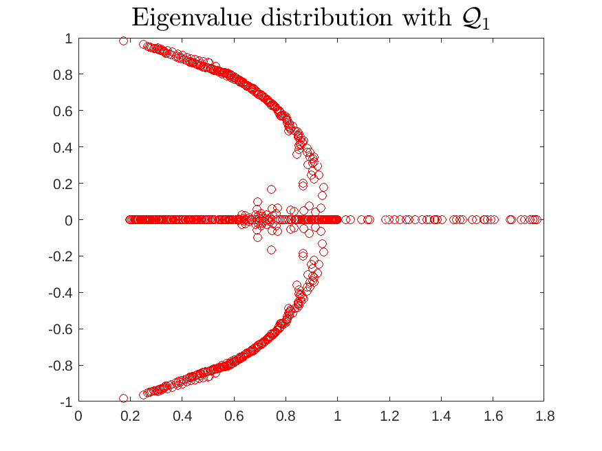
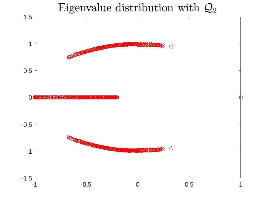
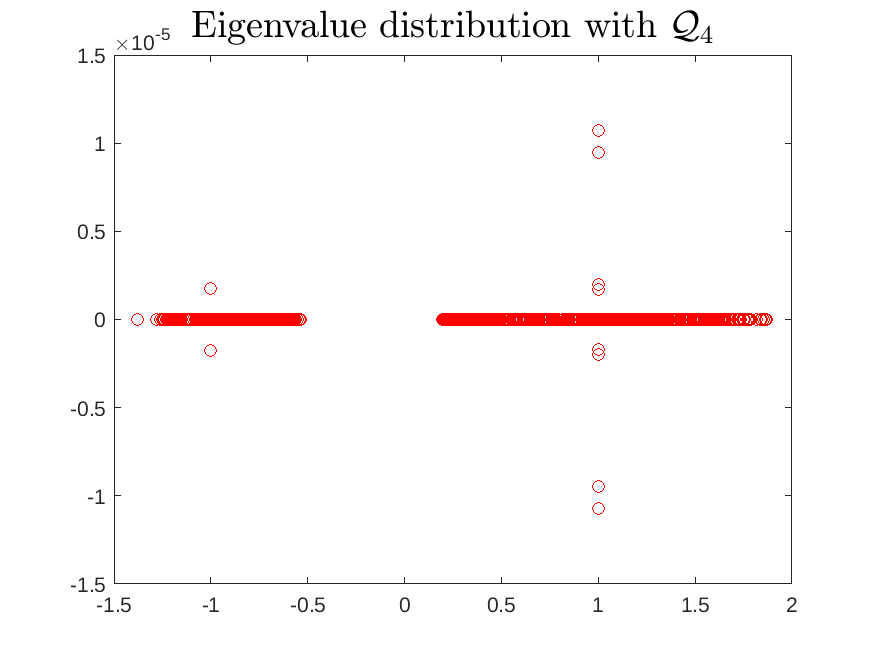
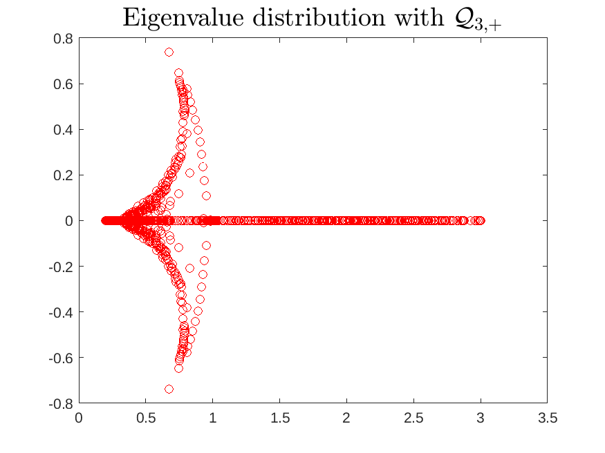
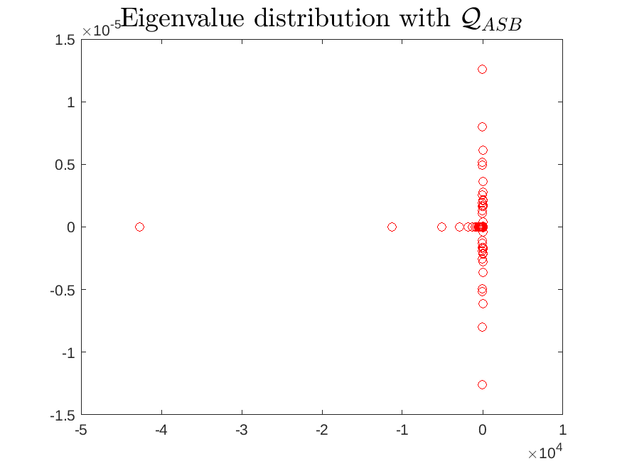
Figure 1: Eigenvalue distribution of the preconditioned matrix with $p=16$ for different preconditioners.

Figure 1 plots the eigenvalue distribution of the preconditioned matrices with the approximation matrices $\widehat{S}$ and $\widehat{X}$. We observe from this figure that the preconditioned matrix with $Q_{3,+}$ has more clustered eigenvalues than the other ones, which can considerably improve the convergence rate of the Krylov subspace iterative methods. Preconditioners ${\mathcal{Q}}_{1}$ and ${\mathcal{Q}}_{5}$ display quite similar eigenvalue distributions (the ideal version have the same eigenvalues). We then remove ${\mathcal{Q}}_{1}$ from the numerical results in view of its slightly higher application cost in comparison with ${\mathcal{Q}}_{5}$. All other proposed preconditioners display also negative eigenvalues, predicting slow GMRES convergence. Finally, the spectral distribution with the ${\mathcal{P}}_{ASB}$ preconditioner, does not seem to be favorable, as it spreads over a wide (real) interval.

The linear system with $\widehat{S}$ is solved exactly by solving two bidiagonal systems with $L_{S}$ and $L_{S}^{T}$, while the system with $\widehat{X}$ is solved, without forming explicitly matrix $\widehat{X}$, by the PCG method accelerated by the incomplete Cholesky factorization of $C\text{diag}(\widehat{S})^{-1}C^{T}$ with a drop tolerance $\tau=10^{-4}$. The work to be done before the beginning of the FGMRES process is described in Algorithm 1 while the application of the preconditioner at each FGMRES iteration is sketched in Algorithm 2, for the preconditioner $Q_{3,+}$.

1:  $\widehat{A}=\text{diag}(A)$,

2:  $\widehat{S}=\text{tridiag}(B\widehat{A}^{-1}B^{T})$

3:  $L_{S}$ is the exact bidiagonal factor of $\widehat{S}$ such that $\widehat{S}=L_{S}L_{S}^{T}$.

4:  Compute $X_{0}=C\text{diag}(\widehat{S})^{-1}C^{T}$ and $M$ its IC factor with drop tolerance $10^{-4}$.

Algorithm 1 Approximations of the blocks before the FGMRES solution.

1:  Split vector $r$ into $r=\begin{bmatrix}r_{1}^{T}&r_{2}^{T}&r_{3}^{T}\end{bmatrix}^{T}$

2:  Solve system $CL_{S}^{-T}L_{S}^{-1}C^{T}w_{3}=r_{3}$ by PCG with preconditioner $MM^{T}$ and $\texttt{tol}_{\texttt{PCG}}=10^{-4}$

3:  $v=C^{T}w_{3}-r_{2}$

4:  $w_{2}=L_{S}^{-T}L_{S}^{-1}v$

5:  $y=r_{1}-B^{T}w_{2}$

6:  Solve $Aw_{1}=y$

7:  Define $w=\begin{bmatrix}w_{1}^{T}&w_{2}^{T}&w_{3}^{T}\end{bmatrix}^{T}$

Algorithm 2 Computation of $w=\text{$Q_{3,+}^{-1}$}r$.

Table 1: Numerical results for example 1 with unitary exact solution.

	size	2080	8256	32896	131328	524800	2 098176	8 390656
	$p$	16	32	64	128	256	512	1024
$\mathcal{P}_{D}$	ITS	79	126	132	128	121	117	†
	CPU	0.15	0.83	3.28	13.25	49.90	165.06	†
	RES	0.21e$-05$	0.12e$-06$	0.88e$-08$	0.49e$-09$	0.35e$-10$	0.20e$-11$	†
	ERR	0.88e$-05$	0.64e$-05$	0.10e$-04$	0.11e$-04$	0.12e$-04$	0.11e$-04$	†
$\mathcal{P}_{3}$	ITS	51	83	87	84	80	77	†
	CPU	0.07	0.43	1.62	7.03	26.45	88.69	†
	RES	0.19e$-05$	0.12e$-06$	0.81e$-08$	0.53e$-09$	0.34e$-10$	0.19e$-11$	†
	ERR	0.68e$-05$	0.60e$-05$	0.10e$-04$	0.11e$-04$	0.12e$-04$	0.11e$-04$	†
$\mathcal{Q}_{2}$	ITS	66	98	100	99	95	91	†
	CPU	0.10	0.64	1.94	8.33	31.30	103.49	†
	RES	0.21e$-05$	0.13e$-06$	0.92e$-08$	0.57e$-09$	0.34e$-10$	0.22e$-11$	†
	ERR	0.66e$-05$	0.64e$-05$	0.97e$-05$	0.10e$-04$	0.10e$-04$	0.10e$-04$	†
$\mathcal{Q}_{4}$	ITS	48	81	85	82	79	76	†
	CPU	0.06	0.46	1.56	6.72	25.59	85.84	†
	RES	0.22e$-05$	0.14e$-06$	0.88e$-08$	0.57e$-09$	0.35e$-10$	0.20e$-11$	†
	ERR	0.64e$-05$	0.67e$-05$	0.10e$-04$	0.12e$-04$	0.11e$-04$	0.10e$-04$	†
$\mathcal{Q}_{5}$	ITS	38	57	59	57	54	52	52
	CPU	0.04	0.22	0.93	3.90	14.49	49.81	294.22
	RES	0.21e$-05$	0.14e$-06$	0.86e$-08$	0.53e$-09$	0.34e$-10$	0.19e$-11$	0.12e$-12$
	ERR	0.59e$-05$	0.68e$-05$	0.10e$-04$	0.11e$-04$	0.12e$-04$	0.10e$-04$	0.11e$-04$
$Q_{3,+}$	ITS	30	44	46	45	43	41	39
	CPU	0.03	0.17	0.64	2.68	10.40	35.52	201.87
	RES	0.19e$-05$	0.14e$-06$	0.86e$-08$	0.47e$-09$	0.33e$-10$	0.20e$-11$	0.12e$-12$
	ERR	0.88e$-05$	0.69e$-05$	0.13e$-04$	0.12e$-04$	0.14e$-04$	0.13e$-04$	0.15e$-04$
$\mathcal{P}_{ASB}$	ITS	19	17	16	15	13	12	45
	CPU	0.05	0.03	0.07	0.27	0.84	2.85	177.30
	RES	0.15e$-05$	0.12e$-06$	0.82e$-08$	0.38e$-09$	0.30e$-10$	0.16e$-11$	0.13e$-12$
	ERR	0.39e$-05$	0.31e$-05$	0.33e$-05$	0.25e$-05$	0.32e$-05$	0.26e$-05$	0.56e$-05$
†: GMRES memory overflow

The numerical results corresponding to the block preconditioned FGMRES for Example 1 are given in Tables 1 (using the right hand side as $b=\mathcal{A}e$) and 2 where an exact random solution is employed.

We run FGMRES with all preconditioners for problems with $p=\{16,32,64,128,256,512,1024\}$ ending up with a problem with more than $8$ million unknowns. To obtain a relative error of (roughly) the same order of magnitude we adjusted the tolerance as

$$\texttt{tol}=\dfrac{10}{N^{2}},\qquad N=n+m+l.$$

Table 2: Numerical results for Example 1 with random exact solution.

	size	2080	8256	32896	131328	524800	2 098176	8 390656
	$p$	16	32	64	128	256	512	1024
$\mathcal{P}_{D}$	ITS	89	147	156	156	152	150	†
	CPU	0.13	0.90	4.31	16.58	61.67	257.74	†
	RES	0.20e$-05$	0.14e$-06$	0.85e$-08$	0.51e$-09$	0.35e$-10$	0.21e$-11$	†
	ERR	0.83e$-05$	0.71e$-05$	0.73e$-05$	0.73e$-05$	0.87e$-05$	0.83e$-05$	†
$\mathcal{P}_{3}$	ITS	58	97	103	101	100	97	†
	CPU	0.06	0.48	1.98	8.32	32.34	128.20	†
	RES	0.20e$-05$	0.11e$-06$	0.83e$-08$	0.57e$-09$	0.33e$-10$	0.22e$-11$	†
	ERR	0.87e$-05$	0.51e$-05$	0.72e$-05$	0.80e$-05$	0.78e$-05$	0.84e$-05$	†
$\mathcal{Q}_{2}$	ITS	74	114	118	117	114	112	†
	CPU	0.07	0.61	2.21	9.67	38.40	146.92	†
	RES	0.21e$-05$	0.13e$-06$	0.87e$-08$	0.52e$-09$	0.35e$-10$	0.22e$-11$	†
	ERR	0.59e$-05$	0.57e$-05$	0.71e$-05$	0.70e$-05$	0.81e$-05$	0.83e$-05$	†
$\mathcal{Q}_{4}$	ITS	55	96	103	103	100	98	†
	CPU	0.06	0.50	1.93	8.46	33.27	126.98	†
	RES	0.22e$-05$	0.14e$-06$	0.79e$-08$	0.47e$-09$	0.34e$-10$	0.22e$-11$	†
	ERR	0.67e$-05$	0.63e$-05$	0.66e$-05$	0.65e$-05$	0.79e$-05$	0.80e$-05$	†
$\mathcal{Q}_{5}$	ITS	43	66	69	68	66	65	60
	CPU	0.04	0.29	1.01	4.70	18.38	70.22	450.92
	RES	0.18e$-05$	0.12e$-06$	0.80e$-08$	0.50e$-09$	0.35e$-10$	0.22e$-11$	0.14e$-12$
	ERR	0.57e$-05$	0.54e$-05$	0.67e$-05$	0.69e$-05$	0.83e$-05$	0.86e$-05$	0.85e$-05$
$Q_{3,+}$	ITS	33	51	54	53	52	52	51
	CPU	0.03	0.21	0.69	3.14	13.17	49.47	301.68
	RES	0.20e$-05$	0.13e$-06$	0.75e$-08$	0.49e$-09$	0.33e$-10$	0.18e$-11$	0.18e$-12$
	ERR	0.11e$-04$	0.57e$-05$	0.65e$-05$	0.73e$-05$	0.81e$-05$	0.71e$-05$	0.78e$-05$
$\mathcal{P}_{ASB}$	ITS	66	98	113	117	117	116	†
	CPU	0.06	0.41	1.67	7.54	29.38	119.92	†
	RES	0.22e$-05$	0.14e$-06$	0.77e$-08$	0.56e$-09$	0.32e$-10$	0.21e$-11$	†
	ERR	0.65e$-05$	0.96e$-05$	0.16e$-04$	0.22e$-04$	0.21e$-04$	0.22e$-04$	†
†: GMRES memory overflow

From these tables, we see that the preconditioners $\mathcal{Q}_{1}$, $\mathcal{Q}_{5}$ and, particularly, $Q_{3,+}$ outperform the other ones in terms of iteration number and CPU time, being all the proposed preconditioners more convenient than $\mathcal{P}_{D}$ and obtaining FGMRES convergence to the solution of (1.1) in a reasonable number of iterations and CPU time. For the largest problem and random right-hand-side, only preconditioners $Q_{3,+}$ and $\mathcal{Q}_{5}$ could solve the given linear system within the memory of our laptop, due do the small number of iterations they required.

Regarding the $\mathcal{P}_{ASB}$ preconditioner we observe that it is the most performing one when $w\equiv e$, yet not providing convergence in two iterations since its exact version is employed, whereas it reveals not competitive with $Q_{3,+}$ for a random exact solution.

In the next section, we will discuss in detail the eigenvalue distribution of the preconditioner matrix using the inexact version of $Q_{3,+}$ and we leave other inexact version of the proposed preconditioners as a topic for further research. Regarding the complex eigenvalues, we perform an analysis similar to the one in [18], but generalized here for the $3\times 3$ block triangular preconditioner.

4 Eigenvalue analysis of the inexact variants of $Q_{3,+}$

We analyze in this section the eigenvalue distribution of the preconditioned matrix $\mathcal{A}\bar{\mathcal{Q}}^{-1}$, where, in the sequel,

$$\bar{\mathcal{Q}}\equiv\text{$Q_{3,+}$}=\begin{pmatrix}\widehat{A}&B^{T}&0\\ 0&-\widehat{S}&C^{T}\\ 0&0&\widehat{X}\end{pmatrix},$$ (4.1)

with $\widehat{A},\widehat{S}$ and $\widehat{X}$ proper SPD approximations (preconditioners) of $A$, $S$ and $X$, respectively.

The relevant spectral properties of the preconditioned matrix $\mathcal{A}\bar{\mathcal{Q}}^{-1}$ will be given in terms of the eigenvalues of $\widehat{A}^{-1}A,\widehat{S}^{-1}\tilde{S}$ and $\widehat{X}^{-1}\tilde{X}$ where $\tilde{S}=B\widehat{A}^{-1}B^{T}$ and $\tilde{X}=C\widehat{S}^{-1}C^{T}$. To this aim, we define

$$\gamma_{\min}^{A}\equiv\lambda_{\min}(\widehat{A}^{-1}A), \gamma_{\max}^{A}\equiv\lambda_{\max}(\widehat{A}^{-1}A),\qquad\gamma_{A}\in[\gamma_{\min}^{A},\gamma_{\max}^{A}],$$ (4.2)

$$\gamma_{\min}^{S}\equiv\lambda_{\min}(\widehat{S}^{-1}\tilde{S}), \gamma_{\max}^{S}\equiv\lambda_{\max}(\widehat{S}^{-1}\tilde{S}),\qquad\gamma_{S}\in[\gamma_{\min}^{S},\gamma_{\max}^{S}],$$ (4.3)

$$\gamma_{\min}^{X}\equiv\lambda_{\min}(\widehat{X}^{-1}\tilde{X}), \gamma_{\max}^{X}\equiv\lambda_{\max}(\widehat{X}^{-1}\tilde{X}),\qquad\gamma_{X}\in[\gamma_{\min}^{X},\gamma_{\max}^{X}].$$ (4.4)

We will finally make the assumption that $1\in[\gamma_{\min}^{A},\gamma_{\max}^{A}$]. This assumption, very commonly satisfied in practice, will simplify some of the bounds mostly regarding real eigenvalues.

Let

$$\bar{\mathcal{D}}=\begin{pmatrix}\widehat{A}&0&0\\ 0&\widehat{S}&0\\ 0&0&\widehat{X}\end{pmatrix}.$$ (4.5)

Then finding the eigenvalues of $\mathcal{A}\bar{\mathcal{Q}}^{-1}$ is equivalent to solving

$$\bar{\mathcal{D}}^{-\frac{1}{2}}\mathcal{A}\bar{\mathcal{D}}^{-\frac{1}{2}}\mathbf{w}=\lambda\bar{\mathcal{D}}^{-\frac{1}{2}}\bar{\mathcal{Q}}\bar{\mathcal{D}}^{-\frac{1}{2}}\mathbb{w},$$

or

$$\begin{pmatrix}\tilde{A}&R^{T}&0\\ R&0&K^{T}\\ 0&K&0\end{pmatrix}\begin{pmatrix}x\\ y\\ z\end{pmatrix}=\lambda\begin{pmatrix}I&R^{T}&0\\ 0&-I&K^{T}\\ 0&0&I\end{pmatrix}\begin{pmatrix}x\\ y\\ z\end{pmatrix},$$ (4.6)

where $\tilde{A}=\widehat{A}^{-\frac{1}{2}}A\widehat{A}^{-\frac{1}{2}},\>R=\widehat{S}^{-\frac{1}{2}}B\widehat{A}^{-\frac{1}{2}}$ and $K=\widehat{X}^{-\frac{1}{2}}C\widehat{S}^{-\frac{1}{2}}$.

Theorem 5.

Suppose that $A\in\mathbb{R}^{n\times n}$ is symmetric positive definite and $B\in\mathbb{R}^{m\times n}$ and $C\in\mathbb{R}^{l\times m}$ are matrices with full row rank. Let $\widehat{A},\widehat{S}$ and $\widehat{X}$ be the symmetric positive approximations of $A,S$ and $X$, respectively. Assume that $\lambda$ is an eigenvalue of the preconditioned matrix $\mathcal{A}\bar{\mathcal{Q}}^{-1}$ and $(x;y;z)$ is the corresponding eigenvector. If $\Im(\lambda)\neq 0$, then $\lambda$ satisfies

$$|\lambda-1| < \sqrt{1-\gamma^{A}_{\min}},\qquad\qquad\text{if}\ Ky=0,$$

$$|\lambda-1| \leq \sqrt{1-\gamma^{A}_{\min}\frac{\|x\|^{2}}{\|y\|^{2}}},\qquad\text{if}\ Ky\neq 0.$$

Proof.

Let $\lambda$ be an eigenvalue of matrix $\mathcal{A}\bar{\mathcal{Q}}^{-1}$ and $(x;y;z)$ be the corresponding eigenvector such that $\|x\|^{2}+\|y\|^{2}+\|z\|^{2}=1$. It follows from (4.6) that

$$\tilde{A}x-\lambda x=(\lambda-1)R^{T}y,$$ (4.7)

$$Rx-(\lambda-1)K^{T}z=-\lambda y,$$ (4.8)

$$Ky=\lambda z.$$ (4.9)

Since $\widehat{A},\widehat{S}$ and $\widehat{X}$ are SPD, and $B$ and $C$ are matrices with full row rank, then $\tilde{A}$ is SPD and $K$ and $R$ are matrices with full row rank. If $y=0$, from (4.7) we can derive $\tilde{A}x=\lambda x$. Thus, it can be deduced that $\lambda\in[\gamma^{A}_{\min},\gamma^{A}_{\max}]$ and then the eigenvalue $\lambda$ is real. The associated eigenvector for this case is of the form $(x;0;0)$ where $x\neq 0$. Assume now that $\lambda\neq 1$ and $y\neq 0$. The rest of the proof is divided into two cases:

Case I. $Ky=0$. From (4.9), we obtain $z=0$. Multiplying (4.7) by $x^{*}$ on the left and the transposed conjugate of (4.8) by $y$ on the right, we get

$$x^{*}\tilde{A}x-\lambda\|x\|^{2}=(\lambda-1)x^{*}R^{T}y,$$ (4.10)

$$x^{*}R^{T}y=-\bar{\lambda}\|y\|^{2}.$$ (4.11)

Inserting (4.11) into equation (4.10), we have

$$x^{*}\tilde{A}x-\lambda+(\lambda-\bar{\lambda})\|y\|^{2}+|\lambda|^{2}\|y\|^{2}=0.$$ (4.12)

Let $\lambda=a+ib$, then taking the real and imaginary parts of (4.12) apart, we obtain

$$x^{*}\tilde{A}x-a+(a^{2}+b^{2})\|y\|^{2}=0,$$ (4.13)

$$b(2\|y\|^{2}-1)=0.$$ (4.14)

From (4.14), we have $b=0$ or $\|y\|^{2}=\frac{1}{2}$. We assume that $b\neq 0$. From (4.12) and after some simple calculations, we have

$$2x^{*}\tilde{A}x-\lambda-\bar{\lambda}+|\lambda|^{2}=0.$$ (4.15)

Using identity $|\lambda|^{2}-\lambda-\bar{\lambda}=|\lambda-1|^{2}-1$, we obtain $|\lambda-1|^{2}=1-2x^{*}\tilde{A}x$. If $1-\gamma^{A}_{\min}\geq 0$, we deduce that

$$|\lambda-1|^{2}\leq 1-\gamma^{A}_{\min},$$

which implies that

$$1-\sqrt{1-\gamma^{A}_{\min}}\leq\Re(\lambda)\leq 1+\sqrt{1-\gamma^{A}_{\min}}.$$

If $1-\gamma^{A}_{\min}<0$, therefore there exists no $\lambda$ with nonzero imaginary part satisfying the equality in (4.15).

Case II. $Ky\neq 0$. Multiplying (4.7) by $x^{*}$ on the left, the transposed conjugate of (4.8) by $y$ on the right and (4.9) by $z^{*}$ on the left, we derive

$$x^{*}\tilde{A}x-\lambda\|x\|^{2}=(\lambda-1)x^{*}R^{T}y,$$ (4.16)

$$x^{*}R^{T}y-(\bar{\lambda}-1)z^{*}Ky=-\bar{\lambda}\|y\|^{2},$$ (4.17)

$$z^{*}Ky=\lambda\|z\|^{2}.$$ (4.18)

Inserting (4.18) and (4.17) into equation (4.16) and easy manipulations, we get

$$x^{*}\tilde{A}x-\lambda(\|x\|^{2}+\|z\|^{2})+(\lambda^{2}+|\lambda|^{2}-\lambda|\lambda|^{2})\|z\|^{2}+\bar{\lambda}(\lambda-1)\|y\|^{2}=0.$$ (4.19)

Using identity $\|x\|^{2}+\|z\|^{2}=1-\|y\|^{2}$, the above expression becomes

$$x^{*}\tilde{A}x-\lambda+(\lambda-\bar{\lambda}+|\lambda|^{2})\|y\|^{2}+(\lambda^{2}-\lambda|\lambda|^{2}+|\lambda|^{2})\|z\|^{2}=0,$$ (4.20)

and can be equivalently written as

$$x^{*}\tilde{A}x-\lambda+\left(\lambda-\bar{\lambda}+|\lambda|^{2}\right)\|y\|^{2}-\lambda\left(|\lambda|^{2}-(\lambda+\bar{\lambda})\right)\|z\|^{2}=0.$$ (4.21)

In case of complex eigenvalues, we will show that the real quantity

$$\rho=|\lambda|^{2}-(\lambda+\bar{\lambda})=|\lambda-1|^{2}-1=|\lambda|^{2}-2a,$$ (4.22)

is always negative, showing that the complex eigenvalues lie in an open circle with center $(1,0)$ and prescribed radius. Let us write (4.20), exploiting the real and imaginary part,

$$x^{*}\tilde{A}x-a+|\lambda|^{2}\|y\|^{2}-a\rho\|z\|^{2} =0,$$ (4.23)

$$b(-1+2\|y\|^{2}-\rho\|z\|^{2}) =0.$$ (4.24)

If $\lambda$ is complex, then $b\neq 0$ and from (4.24) we obtain

$$\|z\|^{2}=\frac{2\|y\|^{2}-1}{\rho},$$ (4.25)

and substituting it in (4.23) we have

$$0=x^{*}\tilde{A}x-a+|\lambda|^{2}\|y\|^{2}-a(2\|y\|^{2}-1)=x^{*}\tilde{A}x+\|y\|^{2}(|\lambda|^{2}-2a)=x^{*}\tilde{A}x+\|y\|^{2}\rho,$$

from which

$$\rho=-\frac{x^{*}\tilde{A}x}{\|y\|^{2}}.$$ (4.26)

We can rewrite (4.26) as

$$\rho=-\gamma_{A}\frac{\|x\|^{2}}{\|y\|^{2}}\leq-\gamma^{A}_{\min}\frac{\|x\|^{2}}{\|y\|^{2}},\qquad\gamma_{A}=\frac{x^{*}\tilde{A}x}{\|x\|^{2}}.$$

which together with (4.22) completes the proof of the theorem. ∎

In the following, our aim is to characterize the real eigenvalues of the preconditioned matrix not lying in $[\gamma^{A}_{\min},\gamma^{A}_{\max}]$. To this end, we premise two technical lemmas which will be useful for our analysis.

Lemma 1.

([20]) Let $\lambda\notin[\gamma^{A}_{\min},\gamma^{A}_{\max}]$. Then for arbitrary $z\neq 0$, there exists a vector $s\neq 0$ such that

$$\frac{z^{T}(\tilde{A}-\lambda I)^{-1}z}{z^{T}z}=\Big{(}\frac{s^{T}\tilde{A}s}{s^{T}s}-\lambda\Big{)}^{-1}=(\gamma_{A}-\lambda)^{-1},$$

where $\gamma_{A}=\dfrac{s^{T}\tilde{A}s}{s^{T}s}$.

Lemma 2.

Let $p(x)$ be the polynomial defined as

$$p(x)=x^{3}-a_{1}x^{2}+a_{2}x-a_{3},\qquad a_{j}>0,\ j=1,2,3,$$

and let $a=\min\{a_{1},\dfrac{a_{3}}{a_{2}}\}$ and $b=\max\{a_{1},\dfrac{a_{3}}{a_{2}}\}$. Then $p(x)<0,\>\forall x\in(0,a)$ and $p(x)>0,\>\forall x>b.$

Proof.

The statement of the lemma comes from observing that $p(x)$ is the sum of the term $x^{3}-a_{1}x^{2}$ which is negative in $(0,a_{1})$ and positive for $x>a_{1}$ and of the term $a_{2}x-a_{3}$ which is increasing and changes sign once for $x=\dfrac{a_{3}}{a_{2}}.$ ∎

Let, as in the previous lemma, $\gamma_{A}=\dfrac{s^{T}\tilde{A}s}{s^{T}s}$ and define $\gamma_{S}=\dfrac{y^{T}RR^{T}y}{y^{T}y}=\dfrac{y^{T}\widehat{S}^{-1/2}\tilde{S}\widehat{S}^{-1/2}y}{y^{T}y}$, hence $\gamma_{S}\in[\gamma^{S}_{\min},\gamma^{S}_{\max}]$ and $\gamma_{X}=\dfrac{z^{T}KK^{T}z}{z^{T}z}=\dfrac{z^{T}\widehat{S}^{-1/2}\tilde{X}\widehat{S}^{-1/2}z}{z^{T}z}\in[\gamma^{X}_{\min},\gamma^{X}_{\max}]$. We are now able to bound the real eigenvalues of the preconditioned matrix $\mathcal{A}\bar{\mathcal{Q}}^{-1}$. We split the main theorem considering two cases $Ky=0$ and $Ky\neq 0$.

Theorem 6.

If $Ky=0$, then the real eigenvalues of the preconditioned matrix not lying in $[\gamma^{A}_{\min},\gamma^{A}_{\max}]$ satisfy

$$\lambda^{2}-(\gamma_{A}+\gamma_{S})\lambda+\gamma_{S}=0.$$

Moreover the following synthetic bound holds:

$$\min\left\{\gamma^{A}_{\min},\frac{\gamma^{S}_{\min}}{\gamma^{A}_{\max}+\gamma^{S}_{\min}}\right\}\leq\lambda\leq\gamma^{A}_{\max}+\gamma^{S}_{\max}.$$ (4.27)

Proof.

From (4.7), we have

$$x=(\tilde{A}-\lambda I)^{-1}(\lambda-1)R^{T}y.$$ (4.28)

Inserting $x$ into the equation (4.8) yields

$$R(\tilde{A}-\lambda I)^{-1}(1-\lambda)R^{T}y=\lambda y.$$ (4.29)

Multiplying the above equation by $\dfrac{y^{T}}{y^{T}y}$ and using Lemma 1, we derive

$$\lambda^{2}-(\gamma_{A}+\gamma_{S})\lambda+\gamma_{S}=0,$$ (4.30)

The solutions of equation (4.30) are

$$\lambda_{1,2}=\frac{\gamma_{A}+\gamma_{S}\pm\sqrt{(\gamma_{A}+\gamma_{S})^{2}-4\gamma_{S}}}{2}.$$

It is easy to see that

$$\lambda_{1}=\frac{\gamma_{A}+\gamma_{S}+\sqrt{(\gamma_{A}+\gamma_{S})^{2}-4\gamma_{S}}}{2}\leq\gamma_{A}+\gamma_{S}\leq\gamma_{\max}^{A}+\gamma^{S}_{\max}.$$

It is not hard to find that the smallest eigenvalue $\lambda_{2}$ is a decreasing function with respect to $\gamma_{A}$ and it is an increasing with respect to $\gamma_{S}$ if $\gamma_{A}\geq 1$. Therefore, we have

$$\lambda_{2} =\frac{\gamma_{A}+\gamma_{S}-\sqrt{(\gamma_{A}+\gamma_{S})^{2}-4\gamma_{S}}}{2}$$

$$=\frac{2\gamma_{S}}{\gamma_{A}+\gamma_{S}+\sqrt{(\gamma_{A}+\gamma_{S})^{2}-4\gamma_{S}}}\geq\frac{\gamma^{S}_{\min}}{\gamma^{A}_{\max}+\gamma^{S}_{\min}}.$$

From the above discussion, we have proved that the real eigenvalues satisfy

$$\frac{\gamma^{S}_{\min}}{\gamma^{A}_{\max}+\gamma^{S}_{\min}}\leq\lambda\leq\gamma^{A}_{\max}+\gamma^{S}_{\max}.$$ (4.31)

∎

Before developing bound on the real eigenvalues of the preconditioned matrix in the general case we state the following Lemma.

Lemma 3.

Let $\zeta\in\mathbb{R}$ be either $0<\zeta<\min\left\{\gamma_{\min}^{A},\dfrac{\gamma_{\min}^{S}}{\gamma_{\max}^{A}+\gamma_{\min}^{S}}\right\}$ or $\zeta\geq\gamma_{\max}^{A}+\gamma_{\max}^{S}$. Then the symmetric matrix

$$Z(\zeta)=(1-\zeta)R(\zeta I-\tilde{A})^{-1}R^{T}+\zeta I,$$ (4.32)

has either all positive or all negative eigenvalues.

Proof.

Let $w$ be a nonzero vector. Multiplying (4.32) by $\dfrac{w^{T}}{w^{T}w}$ on the left and by $w$ on the right and applying Lemma 1, since $\zeta I-\tilde{A}$ has all positive or all negative eigenvalues, yields

$$\frac{w^{T}Zw}{w^{T}w} = (1-\zeta)\frac{w^{T}R(\zeta I-\tilde{A})^{-1}R^{T}w}{w^{T}w}+\zeta=\quad(\text{setting}\ z=R^{T}w)$$ (4.33)

$$= (1-\zeta)\frac{z^{T}(\zeta I-\tilde{A})^{-1}z}{z^{T}z}\frac{w^{T}RR^{T}w}{w^{T}w}+\zeta=$$

$$= \frac{1-\zeta}{\zeta-\gamma_{A}}\gamma_{S}+\zeta.$$

The Rayleigh quotient associated to $Z(\zeta)$, namely the function $h(\zeta)=\dfrac{1-\zeta}{\zeta-\gamma_{A}}\gamma_{S}+\zeta$ can not be zero under the hypotheses on $\zeta$. In fact,

$$h(\zeta)=0\Longrightarrow\zeta^{2}-(\gamma_{A}+\gamma_{S})\zeta+\gamma_{S}=0,$$ (4.34)

and applying (4.31) we obtain the desired result. ∎

The next theorem provides bounds on the real eigenvalues of the preconditioned matrix $\mathcal{A}\bar{\mathcal{Q}}^{-1}$ in the general case.

Theorem 7.

Let $\lambda\in\mathbb{R}$ and $\lambda\notin\left[\min\left\{\gamma_{\min}^{A},\dfrac{\gamma_{\min}^{S}}{\gamma_{\max}^{A}+\gamma_{\min}^{S}}\right\},\gamma_{\max}^{A}+\gamma_{\max}^{S}\right]$. Then the remaining real eigenvalues of the preconditioned matrix $\mathcal{A}\bar{\mathcal{Q}}^{-1}$ satisfy

$$\lambda^{3}-(\gamma_{A}+\gamma_{S}+\gamma_{X})\lambda^{2}+(\gamma_{S}+\gamma_{X}+\gamma_{A}\gamma_{X})\lambda-\gamma_{A}\gamma_{X}=0.$$ (4.35)

Moreover the following synthetic bound holds:

$$\min\left\{\dfrac{\gamma_{\min}^{S}}{\gamma_{\max}^{A}+\gamma_{\min}^{S}},\frac{\gamma_{\min}^{A}\gamma_{\min}^{X}}{\gamma_{\min}^{X}+\gamma^{S}_{\max}+\gamma_{\min}^{A}\gamma_{\min}^{X}}\right\}\leq\lambda\leq\gamma_{\max}^{A}+\gamma_{\max}^{S}+\gamma_{\max}^{X}.$$ (4.36)

Proof.

The equation (4.7) can be written as

$$x=(1-\lambda)(\lambda I-\tilde{A})^{-1}R^{T}y.$$ (4.37)

When we insert this into the second equation in (4.8), we obtain

$$Z(\lambda)y=(\lambda-1)K^{T}z,$$ (4.38)

where $Z(\lambda)=(1-\lambda)R(\lambda I-\tilde{A})^{-1}R^{T}+\lambda I$. The hypotheses on $\lambda$ allow to use Lemma 3 which guarantee the matrix $Z(\lambda)$ is either SPD or symmetric negative definite. Hence, obtaining $y=(\lambda-1)Z(\lambda)^{-1}K^{T}z$ from the previous equation and substituting in (4.9) yields

$$\left[K(\lambda-1)Z(\lambda)^{-1}K^{T}-\lambda I\right]z=0.$$ (4.39)

Premultiplying by $z^{T}$on the left and dividing by $z^{T}z$ yields

$$\frac{z^{T}K(\lambda-1)Z(\lambda)^{-1}K^{T}z}{z^{T}z}-\lambda=0.$$ (4.40)

Setting $w=K^{T}z$, we can obtain

$$(\lambda-1)\frac{w^{T}Z(\lambda)^{-1}w}{w^{T}w}\frac{z^{T}KK^{T}z}{z^{T}z}-\lambda=0.$$ (4.41)

Denoted the vector $u=Z(\lambda)^{-1/2}w$, the equation (4.41) becomes

$$(\lambda-1)\frac{u^{T}u}{u^{T}Z(\lambda)u}\frac{z^{T}KK^{T}z}{z^{T}z}-\lambda=0.$$ (4.42)

Using now the relation (4.33) in Lemma 3, we get

$$\frac{\lambda-1}{\frac{1-\lambda}{\lambda-\gamma_{A}}\gamma_{S}+\lambda}\gamma_{X}-\lambda=0.$$ (4.43)

After simple algebra we are left with the following polynomial cubic equation

$$q(\lambda)\equiv\lambda^{3}-(\gamma_{A}+\gamma_{S}+\gamma_{X})\lambda^{2}+(\gamma_{S}+\gamma_{X}+\gamma_{A}\gamma_{X})\lambda-\gamma_{A}\gamma_{X}=0.$$ (4.44)

Applying Lemma 2 to this cubic polynomial we have

$$a=\frac{\gamma_{A}\gamma_{X}}{\gamma_{X}+\gamma_{S}+\gamma_{A}\gamma_{X}},\qquad b=\gamma_{A}+\gamma_{S}+\gamma_{X}.$$

In this case it is easily verified that $a<b$ from which we have that $a<\lambda<b$ and the statement of the theorem results by observing that the lower bound is an increasing function of both $\gamma_{A}$ and $\gamma_{K}$ and decreasing on $\gamma_{S}$. ∎

Check of the bounds in Theorems 6 and 7. Figure 2 displays in depth the eigenvalue distribution of preconditioned matrix $\bar{\mathcal{Q}}^{-1}\mathcal{A}$.

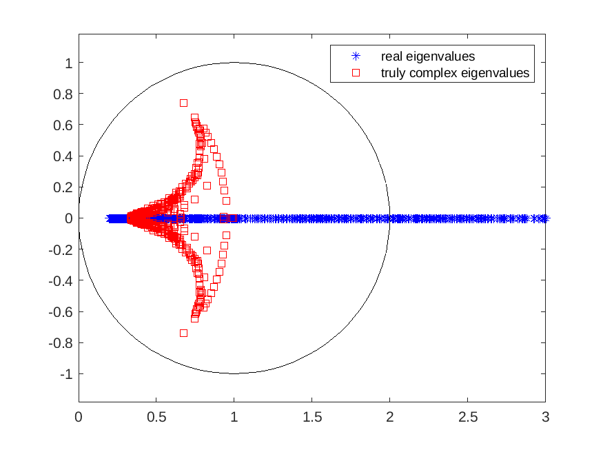
Figure 2: Eigenvalue distribution of preconditioned matrix $\bar{\mathcal{Q}}^{-1}\mathcal{A}$ for Example 1 with $p=16$.

• The complex eigenvalues of the preconditioned matrix $\bar{\mathcal{Q}}^{-1}\mathcal{A}$ fall in the open circle with center (1,0) and radius 1;

• Regarding the real eigenvalues, the results are summarized in the following table:

  $\min\{\lambda,\lambda\in\mathbb{R}\}$	$\max\{\lambda,\lambda\in\mathbb{R}\}$	Lower bound (4.36)	Upper bound (4.36)
  0.1982	3.0019	0.1342	6.2110

In the next section, we will perform a more accurate eigenvalues analysis of the preconditioned matrix with the $\bar{\mathcal{Q}}$ preconditioner, under additional hypotheses.

5 Further characterization of real eigenvalues

We will now consider a simplified preconditioner in which the only approximation is provided by $\widehat{A}\neq A$, whereas $\widehat{S}=B\widehat{A}^{-1}B^{T}\equiv\tilde{S}$ and $\widehat{X}=C\widehat{S}^{-1}C^{T}\equiv\tilde{X}$. Note that $RR^{T}=I_{m}$ and $KK^{T}=I_{l}$.

Theorem 8.

Let $\widehat{S}\equiv\tilde{S}$ and $\widehat{X}\equiv\tilde{X}$. Then any real eigenvalue $\lambda$ of $\mathcal{A}\bar{\mathcal{Q}}^{-1}$ is bounded by

$$\min\left\{\lambda^{+}(\gamma^{A}_{\min}),\gamma^{A}_{\min},\frac{1}{\gamma^{A}_{\max}+1}\right\}\leq\lambda\leq\max\{\lambda^{+}(\gamma^{A}_{\max}),\gamma^{A}_{\max}+1\},$$

where $\lambda^{+}(.)$ is the (unique) positive root of the equation

$$\lambda^{3}-(2+\gamma_{A})\lambda^{2}+(2+\gamma_{A})\lambda-\gamma_{A}=0.$$

Moreover, the following more synthetic bound holds:

$$\dfrac{\gamma^{A}_{\min}}{2}\leq\lambda\leq\gamma^{A}_{\max}+1.$$ (5.1)

Proof.

For this simplified preconditioner we have $\gamma_{S}\equiv 1$ and $\gamma_{X}\equiv 1$. In this case the equation (4.35) becomes

$$p(\lambda;\gamma_{A})\equiv\lambda^{3}-(2+\gamma_{A})\lambda^{2}+(2+\gamma_{A})\lambda-\gamma_{A}=0,$$ (5.2)

for all real

$$\lambda\notin\left[\min\left\{\gamma_{\min}^{A},\dfrac{1}{1+\gamma_{\max}^{A}}\right\},1+\gamma_{\max}^{A}\right].$$ (5.3)

The cubic polynomial equation (5.2) can be written as

$$p(\lambda;\gamma_{A})\equiv\lambda\Big{(}(\lambda-1)^{2}+1\Big{)}-\gamma_{A}(\lambda^{2}-\lambda+1)=0,$$ (5.4)

showing that the function $g(x)\equiv p(\lambda;x)$ is decreasing for each $x\geq 0$ and therefore the position of the largest positive root of (5.4) is increasing. Moreover it is easy to show that for every $\gamma_{A}>0$, there is a unique positive root to the equation $p(\lambda;\gamma_{A})=0$. In fact

$$p(0;\gamma_{A})=-\gamma_{A}<0,\quad p^{\prime}(0;\gamma_{A})=2+\gamma_{A},\qquad p^{\prime}(\tilde{\lambda};\gamma_{A})=0,\quad\tilde{\lambda}=\frac{\gamma_{A}+2-\sqrt{\gamma_{A}^{2}+\gamma_{A}-2}}{3},$$

so that if $\gamma_{A}<1$, the polynomial $p$ is increasing for $\lambda>0$ and it takes a local maximum in $\tilde{\lambda}$ if $\gamma_{A}>1$ in which, however, $p(\tilde{\lambda};\gamma_{A})<p(\tilde{\lambda};1)=0$. Combining all these facts we finally have

$$\lambda^{+}(\gamma^{A}_{\min})\leq\lambda\leq\lambda^{+}(\gamma^{A}_{\max}),$$

where $\lambda^{+}(\gamma_{A})$ refers to the unique positive solution of $p(\lambda;\gamma_{A})=0$, and the thesis holds by observing that $p(\gamma^{A}_{\min};\gamma^{A}_{\min})>0\Longrightarrow\lambda^{+}(\gamma^{A}_{\min})<\gamma^{A}_{\min}$ and $p(\gamma^{A}_{\max};\gamma^{A}_{\max})<0\Longrightarrow\lambda^{+}(\gamma^{A}_{\max})>\gamma^{A}_{\max}$.

Also the second part of the theorem holds since $p\left(\dfrac{\gamma^{A}_{\min}}{2};\gamma^{A}_{\min}\right)=-\dfrac{{(\gamma^{A}_{\min})}^{3}}{8}<0$, then $\lambda^{+}(\gamma^{A}_{\min})>\dfrac{\gamma^{A}_{\min}}{2}$. Moreover, from $p\left(\gamma^{A}_{\max}+1;\gamma^{A}_{\max}\right)=1>0$, we have that $\lambda^{+}(\gamma^{A}_{\max})<\gamma^{A}_{\max}+1$. Combining this with (5.3) and observing that $\dfrac{\gamma^{A}_{\min}}{2}<\dfrac{1}{\gamma^{A}_{\max}+1}$, we conclude the proof.

∎

Remark 8.

Note that we could have applied directly Lemma 2 to equation (5.2), obtaining the following bounds

$$\frac{\gamma_{\min}^{A}}{2+\gamma_{\min}^{A}}\leq\lambda\leq\gamma_{\max}^{A}+2,$$

which are looser than those proved in Theorem 8.

Check of the bounds in Theorem 8. The following example is given to assess the theoretical results developed in Theorem 8.

Example 2.

Consider the linear system (1.1) with the block matrices are randomly generated by the following MATLAB code:

⬇

n = 100; m = 80; l = 60;

z = 1+10*rand(1); w = z*rand(n,1); w = 0.1+sort(w); w(1:10) = w(1);

A = diag(w); B = rand(m,n); C = rand(l,m);

In this example, matrix $A$ is diagonal with a random eigenvalue distribution in $[0.1,11]$ and $\widehat{A}=I$.

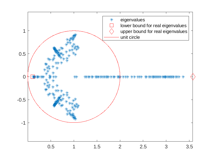
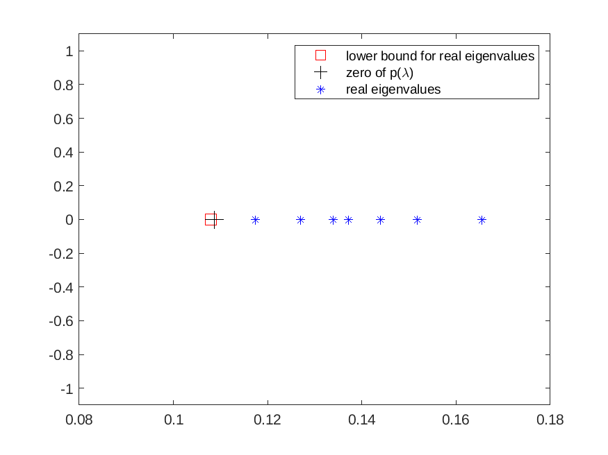
Figure 3: Eigenvalue distribution of the preconditioned matrix $\bar{\mathcal{Q}}^{-1}\mathcal{A}$ for Example 2. Left panel: real eigenvalues – blue asterisks, complex eigenvalues – red circles, upper bound by (5.1) – red diamond. Right panel: smallest eigenvalues compared with the two lower bounds of Theorem 8.

In Figure 3 (left) we show the whole spectrum of the preconditioned matrix $\bar{\mathcal{Q}}^{-1}\mathcal{A}$ together with the bounds for the real eigenvalues. In Figure 3 (right) a zoom of the smallest (real) eigenvalues is provided showing that both the lower bounds, namely $\gamma_{\min}^{A}$ (red box) and $\lambda^{+}$ (black plus) are smaller, yet very close, than the smallest real eigenvalue of the preconditioned matrix. The results of this experiment as well as the observation of the figures point out that:

• The complex eigenvalues of the related preconditioned matrix are located in a circle centered at (1, 0) with radius 1;

• The real eigenvalues lie in the real interval $[0.1024,3.373]$;

• Here $\dfrac{\gamma^{A}_{\min}}{2}=0.1003,\ \lambda^{+}=0.1008$ and $\gamma^{A}_{\max}+1=3.552$

We can appreciate the closeness of the bounds to the endpoints of the real eigenvalue interval.

6 Conclusions

In this work, we have considered a number of exact block preconditioners, developing the spectral distribution of the corresponding preconditioned matrices, for a class of double saddle point problems. Some numerical experiments are performed, which show the good behavior of the preconditioned FGMRES method using an inexact counterpart of these preconditioner, in comparison with other preconditioners from the literature.

We have then concentrated on the inexact variants of a specific block triangular preconditioner, performing a complete spectral analysis and relating the eigenvalue distribution of the preconditioned matrix with the extremal eigenvalues of the (symmetric and positive definite) preconditioned (1,1) block and the Schur complement matrices. Numerical tests are reported which confirm the validity of the developed theoretical bounds.

Future work is aimed at generalizing this work to provide the eigenvalue distribution of more general double saddle-point matrices, in particular those with nonzero $(2,2)$ and $(3,3)$ blocks, and to test them on a wide number of realistic applications, such as, e.g., coupled poromechanical models [21], and the coupled Stokes-Darcy equation [10].

References

- [1] J.-Y. Yuan, Numerical methods for generalized least squares problems, J. Comput. Appl. Math., 66 (1996), pp. 571–584.
- [2] D.-R. Han, X.-M. Yuan, Local linear convergence of the alternating direction method of multipliers for quadratic programs, SIAM J. Numer. Anal., 51 (2013), pp. 3446–3457.
- [3] S. Rhebergen, G.N. Wells, A.J. Wathen, R.F. Katz, Three-field block preconditioners for models of coupled magma/mantle dynamics, SIAM J. Sci. Comput., 37 (2015), pp. A2270–A2294.
- [4] Z.-M. Chen, Q. Du, J. Zou, Finite element methods with matching and nonmatching meshes for Maxwell equations with discontinuous coefficients, SIAM J. Numer. Anal., 37 (2000), pp. 154–1570.
- [5] P. Monk, Analysis of a finite element method for Maxwell’s equations, SIAM J. Numer. Anal., 29 (1992), pp. 714–729.
- [6] M. Cai, M. Mu, J. Xu, Preconditioning techniques for a mixed Stokes/Darcy model in porous media applications, Comput. Appl. Math., 233 (2009), pp. 346–355.
- [7] F. Chen, B. Ren, On preconditioning of double saddle point linear systems arising from liquid crystal director modeling, Appl. Math. Lett, 136 (2023), 108445.
- [8] P. Chidyagwai, S. Ladenheim, D. B. Szyld, Constraint preconditioning for the coupled Stokes-Darcy system, SIAM J. Sci. Comput., 38, (2016), pp. A668—A690.
- [9] F.P.A. Beik, M. Benzi, Iterative methods for double saddle point systems, SIAM J. Matrix Anal. Appl., 39 (2018), pp. 902–921.
- [10] F.P.A. Beik, M. Benzi, Preconditioning techniques for the coupled Stokes–Darcy problem: spectral and field-of-values analysis. Numer. Math. 150, 257–298 (2022).
- [11] Y. Cao, Shift-splitting preconditioners for a class of block three-by-three saddle point problems, Appl. Math. Lett., 96 (2019), pp. 40–46.
- [12] S. Bradley, C. Greif, Eigenvalue bounds for double saddle-point systems. IMA Journal of Numerical Analysis, (2023). Published online on 23 December 2022.
- [13] V. Simoncini, D. Szyld, Recent computational developments in Krylov subspace methods for linear systems, Numer. Linear Algebra Appl., 14 (2007), pp. 1–59.
- [14] N. Huang, C.-F. Ma, Spectral analysis of the preconditioned system for the block saddle point problem, Numer. Algor., 81 (2019), pp. 421–444.
- [15] F. Balani Bakrani, M. Hajarian, L. Bergamaschi, Two block preconditioners for a class of double saddle point linear systems, Applied Numerical Mathematics, 190 (2023), pp. 155–167.
- [16] X. Xie, H.B. Li, A note on preconditioning for the block saddle point problem, Comput. Math. Appl., 79 (2020), pp. 3289–3296.
- [17] N. N. Wang, J.-C. Li, On parameterized block symmetric positive definite preconditioners for a class of block three-by-three saddle point problems, Comput. Appl. Math., 405 (2022), 113959.
- [18] V. Simoncini, Block triangular preconditioners for symmetric saddle-point problems, Appl. Numer. Math., 49 (2004), pp. 63–80.
- [19] H. Aslani, D.K. Salkuyeh, F.P.A. Beik, On the Preconditioning of Three-by-Three Block Saddle Point Problems, Filomat, 35 (2021), pp. 5181–5194.
- [20] L. Bergamaschi, On eigenvalue distribution of constraint-preconditioned symmetric saddle point matrices, Numer. Linear Algebra Appl., 19 (2012), pp. 754–772.
- [21] M. Frigo, N. Castelletto, M. Ferronato, Enhanced relaxed physical factorization preconditioner for coupled poromechanics, Comput. Math. Appl., 106 (2022), pp. 27–39.