On efficient computation in active inference
Abstract
Despite being recognized as neurobiologically plausible, active inference faces difficulties when employed to simulate intelligent behaviour in complex environments due to its computational cost and the difficulty of specifying an appropriate target distribution for the agent. This paper introduces two solutions that work in concert to address these limitations. First, we present a novel planning algorithm for finite temporal horizons with drastically lower computational complexity. Second, inspired by Z-learning from control theory literature, we simplify the process of setting an appropriate target distribution for new and existing active inference planning schemes. Our first approach leverages the dynamic programming algorithm, known for its computational efficiency, to minimize the cost function used in planning through the Bellman-optimality principle. Accordingly, our algorithm recursively assesses the expected free energy of actions in the reverse temporal order. This improves computational efficiency by orders of magnitude and allows precise model learning and planning, even under uncertain conditions. Our method simplifies the planning process and shows meaningful behaviour even when specifying only the agent’s final goal state. The proposed solutions make defining a target distribution from a goal state straightforward compared to the more complicated task of defining a temporally informed target distribution. The effectiveness of these methods is tested and demonstrated through simulations in standard grid-world tasks. These advances create new opportunities for various applications.
Keywords Active inference Dynamic programming Stochastic control Reinforcement learning
1 Introduction
How should an organism perceive, learn, and act to ensure survival when born into a new world? How do ‘agents’ eventually learn to exhibit sentient behaviour in nature, such as hunting and navigation?
A prominent framework that approaches these questions is stochastic optimal control (SOC), which determines the best possible set of decisions—given a specific criterion—at any given time and in the face of uncertainty. The fundamental problem that SOC addresses can be defined as follows: When born at time and ahead, an ‘agent’ receives observations from its surrounding ‘environment’. This ‘agent’ not only passively receives observations but also is capable of responding with ‘actions’. Additionally, it may receive information or has inbuilt reward systems that quantify its chance of survival and progress. So, this process may be summarised as a stream of data from the agent’s perspective: . Here, stands for the observation at time , stands for the agent’s action at time , and stands for the ‘reward’ at time from the external environment or agent’s inbuilt reward structure. In this setting, the primary goal of an agent is to
| (1) |
Eq.1 is an optimisation problem, and due to its general structure, it has a vast scope in various disciplines across the sciences. Several fields of research grew around this idea in the past decades, like reinforcement learning (RL) (Sutton and Barto, 2018), control theory (Todorov, 2006, 2009), game theory (Fudenberg and Tirole, 1991; Lu et al., 2020), and economics (Mookherjee, 1984; Von Neumann and Morgenstern, 1944). But in fact, formulating decision-making as utility maximisation originated much earlier in the ethical theory of utilitarianism in 18th-century philosophy (Bentham, 1781; Mill, 1870), and was later applied by Pavlov in the early 20th century to account for animal conditioning (Pavlov, 1927). Many current engineering methods, such as Q-learning (Watkins and Dayan, 1992), build upon the Bellman-optimality principle to learn proper observation-action mappings that maximise cumulative reward. Model-based methods in RL, like Dyna-Q Peng and Williams (1993), employ an internal model of the ‘environment’ to accelerate this planning process Sutton and Barto (2018). Similarly, efficient methods, e.g., which linearly scales with the problem dimensions, emerged in classical control theory to compute optimal actions in similar settings (Todorov, 2006, 2009).
Another critical and complementary research direction is studying systems showing ‘general intelligence’, which abounds in nature. Indeed, we see a spectrum of behaviour in the natural world that may or may not be accountable by the rather narrow goal of optimising cumulative reward. By learning more about how the brain produces sentient behaviour, we can hope to accelerate the generation of artificial general intelligence (Goertzel, 2014; Gershman, 2023). This outlook motivates us to look into the neural and cognitive sciences, where an integral theory is the free energy principle (FEP), which brings together Helmholtz’s early observations of perception with more recent ideas from statistical physics and machine learning (Feynman, 1998; Dayan et al., 1995) to attempt a mathematical description of brain function and behaviour in terms of inference that has the potential of unifying many previous theories on the subject, including but not limited to cumulative reward maximisation (Friston, 2010; Friston et al., 2022; Da Costa et al., 2023).
In the last decade, the FEP has been applied to model and generate biological-like behaviour under the banner of active inference (Da Costa et al., 2020). Active inference has since percolated into many adjacent fields owing to its ambitious scope as a general modelling framework for behaviour (Pezzato et al., 2023; Oliver et al., 2022; Deane et al., 2020; Rubin, 2020; Fountas et al., 2020; Matsumoto et al., 2022). In particular, several recent experiments posit active inference as a promising approach to optimal control and explainable and transparent artificial intelligence Friston et al. (2009); Friston (2012); Sajid et al. (2021a); Mazzaglia et al. (2022); Millidge et al. (2020); Albarracin et al. (2023). In this article, we consider active inference as an approach to stochastic control, its current limitations, and how they can be overcome with dynamic programming and the adequate specification of a target distribution.
In the following three sections, we consider the active inference framework, discuss existing ideas accounting for perception, planning and decision-making—and identify their limitations. Next, in Section 5, we show how dynamic programming can address these limitations by enabling efficient planning and can scale up existing methods. We formalise these ideas in a practical algorithm for partially observed Markov decision processes (POMDP) in Section5.1. Then we discuss the possibility of learning the agent’s preferences by building upon Z-learning (Todorov, 2006) in Section 6. We showcase these innovations with illustrative simulations in Section 8.
2 Active inference as biologically plausible optimal control
The active inference framework is a formal way of modelling the behaviour of self-organising systems that interface with the external world and maintain a consistent form over time Friston et al. (2021); Kaplan and Friston (2018); Kuchling et al. (2020). The framework assumes that agents embody generative models of the environment they interact with, on which they base their (intelligent) behaviour (Tschantz et al., 2020; Parr and Friston, 2018). The framework, however, does not impose a particular structure on such models. Here, we focus on generative models in the form of partially observed Markov decision processes (POMDPs) for their simplicity and ubiquitous use in the optimal control literature Lovejoy (1991); Shani et al. (2013); Kaelbling et al. (1998). In the next section, we discuss the basic structure of POMDPs and how the active inference framework uses them.
2.1 Generative models using POMDPs
Assuming agents have a discrete representation of their surrounding environment, we turn to the POMDP framework (Kaelbling et al., 1998). POMDPs offer a fairly expressive structure to model discrete state-space environments where parameters can be expressed as tractable categorical distributions. The POMDP-based generative model can be formally defined as a tuple of finite sets :
-
is a set of hidden states () causing observations .
-
is a set of observations, where , in the fully observable setting. In a partially observable setting, .
-
is a set of actions () Eg: .
-
encodes the one-step transition dynamics, i.e., the probability that when action is taken while being in state (at time ) results in at time .
-
encodes the likelihood mapping, for the partially observable setting.
-
Encodes the prior of the agent about the hidden state factor .
-
Encodes the prior of the agent about actions .
In a POMDP, the hidden states () generate observations () through the likelihood mapping () in the form of a categorical distribution, . is a collection of square matrices , where represents transition dynamics ): The transition matrix () determines the dynamics of given the agent’s action as . In and , is represented as a one-hot vector that is multiplied through regular matrix multiplication 222One-hot is a group of bits among which the legal combinations of values are only those with a single high (1) bit and all the others low (0). Here, the bit (1) is allocated to the state . The Markovianity of POMDPs means that state transitions are independent of history (i.e. state only depends upon the state-action pair and not etc.).
In summary, the generative model can be summarised as follows,
| (2) |
So, from the agent’s perspective, when encountering a stream of observations in time, such as , as a consequence of performing a stream of actions , the generative model quantitatively couples and quantifies the causal relationship from action to observation through some assumed hidden states of the environment. These are called ‘hidden’ states because, in POMDPs, the agent cannot observe them directly. Based on this representation, an agent can now attempt to optimise its actions to keep receiving preferred observations. Currently, the generative model has no concept of ‘preference’ and ‘goal’ (Bruineberg et al., 2018). Rather than attempting to maximise cumulative reward from the environment, active inference agents minimise the ‘surprise’ of encountered observations (Sajid et al., 2021a, b). We look at this idea closely in the next section.
2.2 Surprise and free energy
The surprise of a given observation in active inference (Friston, 2019; Sajid et al., 2021a) is defined through the relation
| (3) |
Please note that the agent does not have access to the true probability of an observation: . However, the internal generative model expects an observation with a certain probability , which quantifies surprise in Eq.3. Minimising surprise directly requires the marginalisation of the generative model, i.e., , which is often computationally intractable due to the large size of the state-space (Blei et al., 2017; Sajid et al., 2022a). Since is a convex function, we can solve this problem by defining an upper-bound to surprise using Jensen’s inequality 333Jensen’s inequality: If is a random variable and is a convex function, .:
| (4) |
The newly introduced term is often interpreted as an (approximate posterior) belief about the (hidden) state: . This upper bound (F) is called the variational free energy (VFE) (it is also commonly known as evidence lower bound – ELBO (Blei et al., 2017) 444The connection between the two lies in the fact that they are essentially equivalent up to a constant (the log evidence), but with opposite signs. In other words, minimizing VFE is equivalent to maximizing the ELBO. Formally this is: ). So, by optimising the belief to minimise the variational free energy (F), an agent is capable of minimising the surprise or at least maintain it bounded at low values.
How is this formulation useful for stochastic control?
Imagine the agent embodies a biased generative model with ‘goal-directed’ expectations for observations. The goal then becomes to minimise , which can be done through the conjunction of perception, i.e., optimising the belief , or action, i.e., controlling the environment to sample observations that lead to a lower (Tschantz et al., 2020). So, instead of passively inferring what caused observations, the agent starts to ‘actively’ infer, exerting control over the environment using available actions in . The central advantage of this formalism is that there is now only one single cost function () to optimise all aspects of behaviour, such as perception, learning, planning, and decision-making (or action selection). There are related works in the reinforcement literature noting the use of similar information-theoretic metrics for control Rhinehart et al. (2021); Berseth et al. (2019). The following section discusses this feature in detail and further develops the active inference framework.
3 Perception and learning
3.1 Perception
From the agent’s perspective, perception means (Bayes optimally) maintaining a belief about hidden states causing the observations . In active inference, agents optimise the beliefs to minimise . The VFE may be rewritten (from Eq.4), using the identity , as:
| (5) |
Differentiating w.r.t and setting the derivative to zero, we get (see Supplementary A),
| (6) |
Using the above equation, we can evaluate the optimal that minimises555The second derivate of Eq.6 w.r.t to is greater than zero which corresponds to local minima of w.r.t to . using,
| (7) |
This equation provides the (Bayesian) belief propagation scheme, given by
| (8) |
Here, is the softmax function; that is, the exponential of the input that is then normalised so that the output is a probability distribution. Given a real-valued vector in , the i-th element of reads:
| (9) |
where corresponds to the i-th element of . We estimate the first term of Eq.8, i.e. the prior using belief at time , and the action taken at time . Using the transition dynamics operator , we write:
| (10) |
At the first time step, i.e. , we use a known prior about the hidden state to substitute for the term . Similarly, the second term in Eq.8, i.e., the estimate of the hidden state from the observation we gathered from the environment at time can be evaluated as the dot product between the likelihood function and the observation gathered at time . The belief propagation scheme here is shown in the literature to have a degree of biological plausibility in the sense that it can be implemented by a local neuronal message-passing scheme (de Vries and Friston, 2017). The following section discusses the learning of the model parameters.
3.2 Learning
The parameter learning rules of our generative model are defined in terms of the optimised belief about states . In our architecture, the agent uses belief propagation 666We stick to the belief propagation scheme for perception in this paper. However, general schemes like variational message passing may be used to estimate . to best estimate , the belief about (hidden) states in the environment. Given these beliefs, observations sampled, and actions undertaken by the agent, the agent hopes to learn the underlying contingencies of the environment. The learning rules of active inference consist of inferring parameters of , , and at a slower time scale. We discuss such learning rules in detail in the following.
3.2.1 Transition dynamics
Agents learn the transition dynamics, , across time by maintaining a concentration parameter , using conjugate update rules well documented in the active inference literature(Friston et al., 2017; Da Costa et al., 2020; Sajid et al., 2021a) such as:
| (11) |
where is the probability of taking action , is belief the state at time as a consequence of action at , and represents a square matrix of Kronecker product between two vectors and .
Every column of the transition dynamics , can be estimated from column-wise as,
| (12) |
Here, is the i-th column of . represents the mean of the Dirichlet distribution 777Dirichlet distributions are commonly used as prior distributions in Bayesian statistics given that the Dirichlet distribution is the conjugate prior of the categorical distribution and multinomial distribution. We use the mean of the Dirichlet distribution here because we are performing a Bayesian update. Briefly, the mean of a Dirichlet distribution with parameters is given by where . So, in this case, each entry in the estimated transition probabilities is the corresponding entry in , divided by the sum of all entries in the corresponding column of . This normalization ensures that the columns of sum to 1. with parameter .
3.2.2 Likelihood
Similar to the conjugacy update in Eq.11, the Dirichlet parameter () for the likelihood dynamics () is learned over time within trials using the update rule,
| (13) |
Here, is the observation gathered from environment at time , and is the approximate posterior belief about the hidden-state () (Friston et al., 2017; Da Costa et al., 2020).
Like perception and learning, decision-making and planning can also be formulated around the cost function and belief . In the next section, we review in detail existing ideas (Friston et al., 2021; Sajid et al., 2022b) for planning and decision-making. We then identify their limitations and, next, propose an improved architecture.
4 Planning and decision making
4.1 Classical formulation of active inference
Traditionally, planning and decision-making by active inference agents revolve around the goal of minimising the variational free energy of the observations one expects in the future. To implement this, we define a policy space comprising sequences of actions in time. The policy space in classical active inference (Sajid et al., 2021a) is defined as a collection of policies
| (14) |
which are themselves sequences of actions indexed in time; that is, , where is one of the available action in , and is the agent’s planning horizon. is the total number of unique policies defined by permutations of available actions over a time horizon of planning .
To enable goal-directed behaviour, we need a way to quantify the agent’s preference for sample observations . The prior preference for observations is usually defined as a categorical distribution over observations,
| (15) |
So, if the value corresponding to an observation in is the highest, it is the most preferred observation for the agent. Given these two additional parameters ( and ), we can define a new quantity called the expected free energy (EFE) of a policy similar to the definition in (Sajid et al., 2021a; Schwartenbeck et al., 2019; Parr and Friston, 2019) as,
| (16) |
In Eq.(16) above, is the t-th element in , i.e. the action corresponding to time for policy . The term, represents the most likely observation caused by the policy at time . stands for the KL-divergence, which, when minimised, forces the distribution closer towards . This term is also called the "Risk" term, representing the goal-directed behaviour of the agent. The KL-divergence between two distributions, and , is defined as:
| (17) |
and if and only if .
In the second term of Eq.16, stands for the (Shannon) entropy of defined as,
| (18) |
The second term is also called the ‘Expected ambiguity’ term. When the expected entropy of w.r.t the belief is less, the agent is more confident of the state-observation mapping (i.e., ) in its generative model.
Hence, by choosing the policy to make decisions that minimise , the agent minimises ‘Risk’ at the same time and also its ‘Ambiguity’ about the state-observation mapping. Hence, in active inference, decision-making naturally balances the exploration-exploitation dilemma (Triche et al., 2022). We also note that the agent is not optimising but only evaluating and comparing various over different policies in the policy space . Once the best policy is identified, the most simple decision-making rule follows by choosing actions at time , where is the -th element of .
It may already be evident that the above formulation has one fundamental problem: in the stochastic control problems that are commonly encountered in practice, the size of possible action spaces and the time horizons of planning make the policy space too large to be computationally tractable. For example, with eight available actions in and a time horizon of planning , the total number of (definable) policies that need to be considered are () trillion. Even for this relatively small-scale example, this policy space is not computationally tractable to simulate agent behaviour (unless additional decision tree search methods are considered (Fountas et al., 2020; Champion et al., 2021a, b) or policy amortisation Fountas et al. (2020); Çatal et al. (2020)) or by eliminating implausible policy trajectories using Occam’s principle. We now turn to an improved scheme that redefines policy space and planning all together.
4.2 Sophisticated inference
Graduating from the classical definition of policy as a sequence of actions in time, sophisticated inference (Friston et al., 2021) attempts to evaluate the EFE of observation-action pairs at a given time , . Given this joint distribution, an agent can sample actions using the conditional distribution when observing at time ,
| (19) |
Given the prior-preference distribution of an agent , in terms of hidden states , the expected free energy of an observation-action pair is defined as (Friston et al., 2021),
| (20) | |||
| (21) |
We rewrite this equation in a familiar fashion to Eq.16. In the above equation, the agent holds evaluated beliefs about future hidden states given all past actions in the term . Beliefs about hidden states can be extrapolated to observations using the likelihood mapping () as
| (22) |
Also, the prior preference of the agent is defined in terms of hidden states in Eq.20. Now the Eq.20 can be rewritten using mappings like Eq.22 as,
| (23) | |||
| (24) |
Note that the prior preference distribution in the equation above is over observations , . Rewriting Eq.23 in a similar fashion to the previously discussed classical active inference we obtain
| (25) | |||
| (26) |
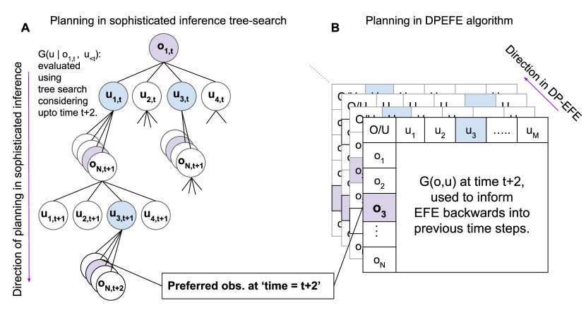
The first two terms can be interpreted the same way as we did for Eq.23 in the previous section. However, the third term in Eq.25 gives rise to a recursive tree-search algorithm, accumulating free energies of the future (as deep as we evaluate forward in time). Such an evaluation is pictorially represented in Fig.1 (A).
While Bellman optimal Da Costa et al. (2021), one unavoidable limitation of the sophisticated inference planning algorithm is that it faces a worse curse of dimensionality for even relatively small planning horizons. For example, to evaluate the goodness of an action within a period of fifteen time-steps into the future, and with eight available actions and a hundred hidden states, requires an exorbitant () calculations, in comparison to () for classical active inference. A simple solution proposed in (Friston et al., 2021) is to eliminate tree search branches by setting a threshold value to predictive probabilities such as in Eq.25. So, for example, when during planning, the algorithm terminates the search over future branches. This restriction significantly reduces the computational time, and a set of ensuing (meaningful) simulations was presented in (Friston et al., 2021).
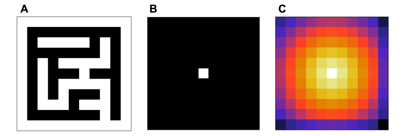
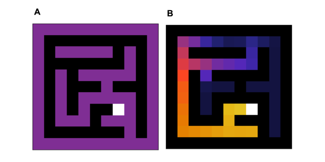
Another limitation is that in all active or sophisticated inference agents to facilitate desirable behaviour, a prior preference needs to be defined by the modeller or learned by the agents Sajid et al. (2021b, 2022c) informing the agent that some states are preferable to others, as demonstrated in Fig.2 (B) for a grid problem given in Fig.2 (A). An informed prior preference enables the agent to solve this navigation task by only planning four or more time steps ahead. It can take action and move towards a ‘more preferred state’ if not the final goal state. However, without such information, the agent is ‘blind’ (cf. Fig.2 (C)) and can only find the optimal move when planning the whole eight-step trajectory for the given grid.
We first noticed this limitation when comparing different active inference schemes to various well-known reinforcement learning algorithms in (Paul et al., 2021) in a fully observable setting (i.e., MDPs). In the next section, we demonstrate how to scale the sophisticated inference scheme using dynamic programming for the general case of POMDP-based generative models.
5 Dynamic programming for evaluating expected free energy
The Bellman optimality principle states that the sub-policy of an optimal policy (for a given problem) must itself will be an optimal policy for the corresponding sub-problem (Sutton and Barto, 2018). Dynamic programming is an optimisation technique that naturally follows the Bellman optimality principle; rather than attempting to solve a problem as a whole, dynamic programming attempts to solve sub-parts of the problem and integrate the sub-solutions into a solution to the original problem. This approach makes dynamic programming scale favourably, as we solve one sub-problem at a time to integrate later. The more we break down the large problem into corresponding sub-problems, the more computationally tractable is the solution.
Inspired by this principle, let us consider a spatial navigation problem that the agent needs to solve in our setting. The optimal solution to this navigation problem is a sequence of individual steps. Our prior preference for the ‘goal state’ is for the end of our time horizon of planning. So, the agent may start planning from the last time step (a step sub-problem) and go backwards to solve the problem. This approach is also called planning by backward induction Zhou et al. (2019).
So, for a planning horizon of (i.e., the agent aims to reach goal state at time ), the EFE of the (last) action for the th time step in a POMDP setting is written as:
| (27) |
The term, is the expected free energy associated with any action , given we are in (hidden) state . This estimate measures how much we believe observations at time will align with our prior preference . Note that, for simplicity, we ignored the ‘expected ambiguity’ term in the equation above, i.e. the uncertainty of state-observation mapping (or likelihood), cf. Eq.25. This does not affect our subsequent derivations; we can always add it as an additional term. The following derivation provided technical details of dynamic programming while focusing only on the ‘risk’ term in .
To estimate , we make use of the prediction about states that can occur at time :
| (28) |
and given the prediction , we write
| (29) | |||
| (30) |
Next, using Eq.28, the corresponding action distribution (for action selection) is calculated at time ,
| (31) |
where we recursively calculate the expected free energy for actions and the corresponding action-distributions for time steps backwards in time,888For times other than , the first term in Eq.32 does not contribute to solving the particular instance if only accommodates preference to a (time-independent) goal-state. However, for a temporally informed , i.e. with a separate preference for reward maximisation at each time step, this term will meaningfully influence action selection.
| (32) |
In the equation above, the second term condenses information about all future observations rather than doing a forward tree search in time. To inform , we consider all possible observation-action pairs that can occur in time and use the previously evaluated . In Eq.32, we evaluate using,
| (33) |
We then map the distribution to the observation space and evaluate using the likelihood mapping . In Eq.33, we assume that actions in time are independent of each other, i.e. is independent of . Even though actions are assumed to be explicitly independent in time, the information (and hence desirability) about actions are also informed backwards in time from the recursive evaluation of expected free energy.
While evaluating the EFE, , backwards in time, we used the action distribution in Eq.31. This action distribution can be directly used for action selection. Given an observation at time , may be sampled 999Precision of action-section may be controlled by introducing a positive constant inside the softmax function in Eq.31. The higher the constant, the higher the chance of selecting the action with less EFE. from,
| (34) |
In the next section, we summarise the above formulation as a novel active inference algorithm useful for modelling intelligent behaviour in sequential POMDP settings.
5.1 Algorithmic formulation of DPEFE
Here, we formalise a generic algorithm that can be employed for a sequential POMDP problem. The main algorithm (see Alg.1) works sequentially in time and brings together three different aspects of the agent’s behaviour, namely, perception (inference), planning, and learning.
For planning, that is, to evaluate the expected free energy () for actions (given states) in time, we employ the planning algorithm (See. Alg.2) as a subroutine to Alg.1. In the most general case, the algorithm is initialised with ’flat’ priors for the likelihood function () and transition dynamics (). The algorithm also allows us to equip the agent with a more informed prior about and . Learning in the DPEFE algorithm is setting as a one-hot vector with the encountered goal state. This technique accelerates the parameters’ learning process during trials and improves agent performance. We can also make available the ‘true’ dynamics of the environment to the agent whenever present. With ‘true’ dynamics available at the agent’s disposal, the agent can infer hidden states and plan accurately. The next section discusses a different approach to ameliorating the curse of dimensionality in sophisticated inference. Later, we discuss a potential learning rule for the prior preference distribution inspired by a seminar work in the control theoretic literature.
6 Learning prior preferences
In the previous section, we introduced a practical algorithm solution that speeds up planning in sophisticated inference. The second innovation on offer is to enable learning of preferences such that smaller planning horizons become sufficient for our agent to take optimal actions, as discussed in Fig.2. A seminal work from the literature on control theory proposes using a ‘desirability’ function, scoring how desirable each state is, to compute optimal actions for a particular class of MDPs and, importantly, showing that the planning complexity of computing those actions is linear in time (Todorov, 2006). When the underlying MDP model of the environment is unavailable and the agent needs to take actions based solely on a stream of samples of states and rewards (i.e., ), an online algorithm called Z-learning, inspired from the theoretical developments in (Todorov, 2006), was proposed to solve this problem. Given an optimal desirability function , the optimal control, or policy, is analytically computable. The calculation of does not rely on knowledge of the underlying MDP but instead, on the following online learning rule:
| (35) |
where, is a learning rate that is continuously optimised—see below. These two terms form a weighted average that updates the estimate of , with controlling the balance between the old estimate and the new information.
Inspired by these developments, we write a learning rule for updating which can be useful for the sophisticated inference agent. Given the samples , an agent may learn the parameter online using a rule analogous to Eq.35,
| (36) |
In the above equation, represents the desirability of an observation at time . The value of is updated depending on the reward received and the desirability of the observation received at the next time step .
The learning rate is a time-dependent parameter in Z-learning, as given in the equation below. is a hyperparameter we optimise that influences how fast/slow gets updated over time Todorov (2009):
| (37) |
If is high, the algorithm puts more weight on the new information. If is low, the algorithm puts more weight on the current estimate. Using the update rule in Eq.36 with the learning rate evolving as in (37), the value of evolves over time and may be used to update online, ensuring that is a categorical distribution over observations using the softmax function:
| (38) |
We use the standard grid world environments as shown in Fig.3 for the evaluation of the performance of various agents (more details in the next sections). Fig.6, is a visualisation that represents the learned prior preference (for the grid shown in Fig. 3 (A)) useful for the sophisticated inference agent. With an informed prior preference like this, the agent needs to plan only one time step ahead to navigate the grid successfully. It should be noted that in the DPEFE setting, we fix the prior preference either before a trial or learn it when we encounter the goal as a one-hot vector. We are not learning an informed prior preference for the DPEFE agent in the simulations presented in the paper. The method for learning prior preference discussed in this section holds for any agent, but in our paper, DPEFE is not using this feature to demonstrate its ability to plan deeper. When we aid an active inference algorithm with the learning rule for , a planning horizon of suffices to take desirable actions (i.e. with no deep tree search like in SI or policy space () as in CAIF). With considering only the next time step, (i.e. only the consequence of immediately available actions), planning in all active inference agents (CAIF, SI, and DPEFE) are algorithmically equivalent. In the rest of the paper, we call this agent with planning horizon , which is aided with the learning rule of as active inference AIF (T = 1) agent. In our simulations, we compare the performance of these two approaches (i.e., deep planning with sparse and short-term planning with learning ). An animation that visualises the learning prior preference distribution for the grid over episodes in Fig.2 can be found in this link. In the following section, we discuss and compare the computational complexity of planning between existing and newly introduced schemes.
7 Computational complexity
In this section, we compare the computational complexity in evaluating the expected free energy term, used for planning and decision making, with two other active inference approaches: classical active inference Da Costa et al. (2020),Sajid et al. (2021a), and sophisticated inference Friston et al. (2021).
In classical active inference (Da Costa et al. (2020), Sajid et al. (2021a)), the expected free energy for an MDP (i.e., a fully observable case) is given by,
| (39) |
Here, represents an agent’s prior preference and is equivalent to in an MDP setting. In this paper, is directly defined in terms of the hidden states. To avoid confusion, we always use the notation in this paper regarding the observations .
Similarly, for sophisticated inference (Friston et al., 2021), we have,
| (40) |
In the above equation, we restrict the recursive evaluation of the second term, forward in time, till a ‘planning horizon (T)’ as mentioned in Friston et al. (2021). necessary for ’full-depth planning’ i.e planning to the end of the episode is often required for sparsely defined prior preferences. This is required since the agent would not be able to differentiate the desirability of actions until reaching the last step of the episode through a tree search.
In classical active inference, to evaluate Eq.39, the computational complexity is proportional to: For sophisticated inference, to evaluate Eq.40, the complexity scales proportionally to: The dimensions of the quantities involved are specified in Tab.1. And recall that both Eq.39 and Eq.40 ignore the ‘ambiguity’ term for simplicity.
| Sophisticated inference | Classical active inference | ||
| Term | Dimension | Term | Dimension |
| (cardinality of S) | |||
For evaluating EFE using dynamic programming, the expected free energy for an MDP can be deduced from Eq.32 as,
| (41) |
Since we only evaluate on time-step ahead in Eq.41, even when evaluating backwards in time, the complexity scales as:
8 Simulations results
8.1 Setup
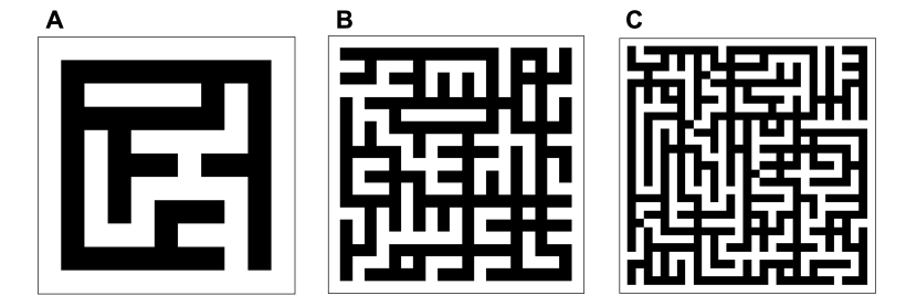
We perform simulations in the standard grid world environment in Fig.3 to evaluate the performance of our proposed algorithms. The agent is born in a random start state at the beginning of every episode and can take one of the four available actions (North, South, East, West) at every time step to advance towards the goal state until the episode terminates either by a time-out (, , and steps for the grids in Fig.3 respectively) or by reaching the goal state. For completeness, we compare the performance of the following algorithms in the grid world:
-
•
Q-learning: a benchmark model-free RL algorithm Watkins and Dayan (1992)
-
•
Dyna-Q: a benchmark model-based RL algorithm improving upon Q-learning Peng and Williams (1993)
-
•
DPEFE algorithm with strictly defined (sparse) (See Sec.5.1)
-
•
Active inference algorithm aided with learning rule for (See Sec.6) and planning horizon of i.e with no deep tree search like in SI, or policy space () as in CAIF. With considering only the next time step, (i.e. only the consequence of immediately available actions) planning in all active inference agents (CAIF, SI, and DPEFE) are algorithmically equivalent. In the rest of the paper, we call this agent with planning horizon aided with the learning rule of as active inference AIF (T = 1) agent.
We perform simulations in deterministic and stochastic grid variations shown in Fig.3. The deterministic variation is a fully observable grid with no noise. So, an agent fully observes the present state—i.e., an MDP setting. Also, the outcomes of actions are non-probabilistic with no noise—i.e., a deterministic MDP setting. In the stochastic variation, we make the environment more challenging to navigate by adding noise in the transitions and noise in the observed state. In this case, the agent faces uncertainty at every time step about the underlying state (i.e., partially observable) and the next possible state (i.e., stochastic transitions)—i.e., a stochastic POMDP setting.
8.2 Summary of results
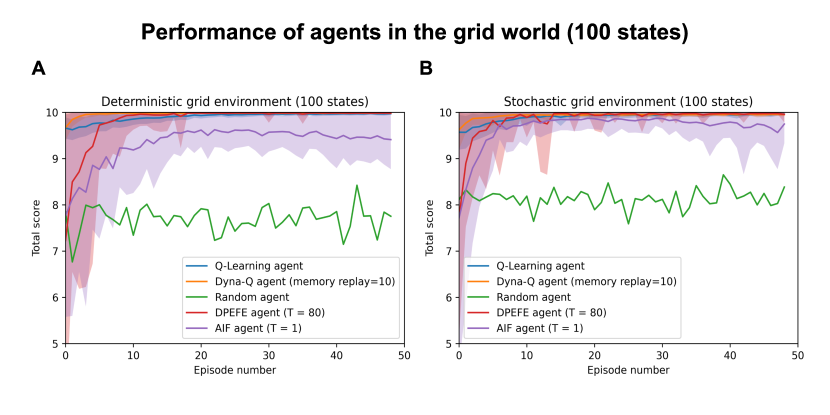
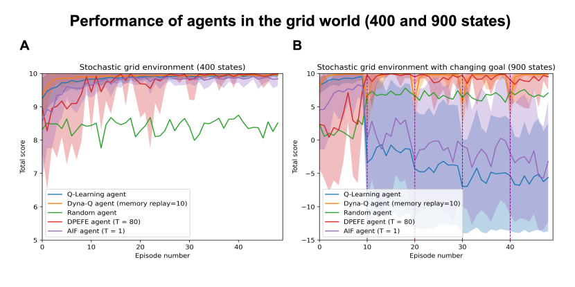
The agents’ performance in this navigation problem is summarised in Fig.4 and Fig.5. Performance is quantified in terms of how quickly an agent learns to solve the grid task, i.e. the total score. The agent receives a reward of ten points when the goal state is reached and a small negative reward for every step taken. The total score hence represents how fast the agent navigated to the goal state for a given episode. The grid has a fixed goal state throughout the episodes in Fig.4 (A, B) and Fig.5 (A). For simulations in Fig.5 (B), the goal state is shifted to another random state every 10 episodes. This setup helps to evaluate the adaptability of agents in the face of changes in the environment. It is clear that during the initial episodes, the agents take longer to reach the goal state but learn to navigate quicker as the episodes unfold. Standard RL algorithms (i.e., Dyna-Q and Q-Learning) are used here to benchmark the performance of active inference agents, as they are efficient state-of-the-art algorithms to solve this sort of task.
In our simulations, the DPEFE algorithm performs at par with the Dyna-Q algorithm with a planning depth of 101010a planning horizon more than any optimal path in this grid. Since the start state is randomized, optimal paths can have many lengths in the grid. A planning depth of ensures that the agent plans enough not to miss the length that needs to be covered in any setting. (See (Fig.4 (A, B), Fig.5 (A)). The DPEFE agent performs even better when we randomised goal-states every episode (Fig.5 (B)). In contrast to online learning algorithms like Dyna-Q, active inference agents can take advantage of the re-definable explicit prior preference distribution . For the AIF(T = 1) agent, we observe that the performance improves over time but is not as good as the DPEFE agent. This is because the AIF(T = 1) agent plans for only one step ahead in our trials by design. We could also observe that the Q-Learning agent performs worse than the random agent and recovers slower than the AIF(T = 1) agent when faced with uncertainty in the goal state. It is a promising direction to optimise the learning of prior preference in the AIF(T = 1) agent, ensuring accuracy in the face of uncertainty. All simulations were performed for trials with different random seeds to ensure the reproducibility of results.
Besides this, we observe a longer time to achieve the goal state for both active inference agents (even longer than the ‘Random agent’) in the initial episodes. This is a characteristic feature of active inference agents, as their exploratory behaviour dominates during the initial trials. The goal-directed behaviour dominates only after the agent sufficiently minimises uncertainty in the model parameters Tschantz et al. (2020).
8.3 Optimising learning rate parameter for AIF (T = 1) agent
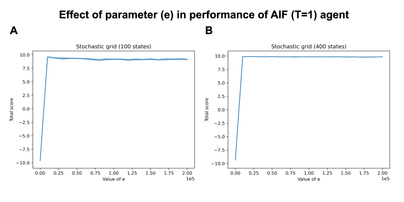
The learning rule proposed for sophisticated inference in Eq.37 requires a (manually) optimised value of for every environment that influences the learning rate . Todorov (2009) inspires this learning rule, where the value of determines how fast the parameter converges for a given trial. The structure of learned is crucial for the active inference agent, as determines how meaningful the planning is for the agent. In Fig.B.1, we plot the performance of the AIF(T = 1) agent as a function of for the grids in Fig. 3. A promising direction for future research is to improve the learning rule based on and fine-tune the method for learning . The observation in Fig.B.1 is that the performance of the AIF(T = 1) agent is not heavily dependent on the value of . We used different values of in AIF(T = 1) agents in all settings in this paper.
8.4 An emphasis on computational complexity
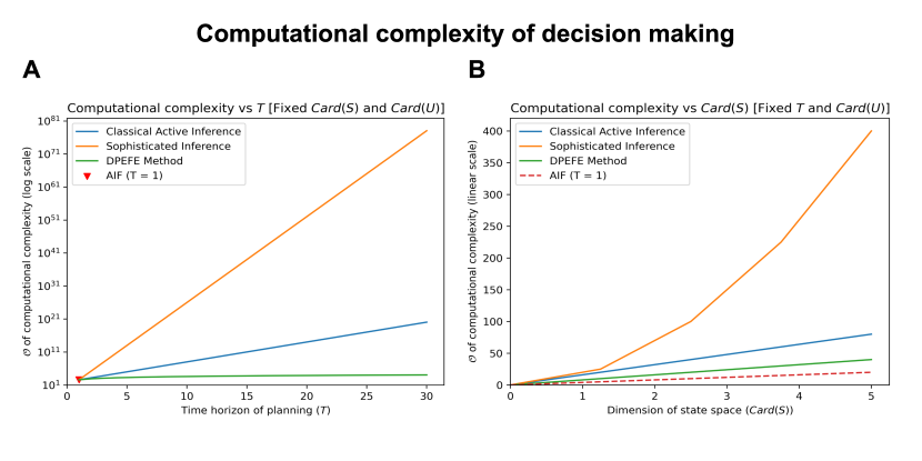
To understand why the classical active inference (CAIF) and SI methods cannot solve these grid environments with the traditional planning method, we provide an exemplar setting in Tab. 2. Consider the small grid as shown in Fig.3 with , , . Tab.2 summarises the computational complexity of simulating various active inference agents for this small grid world problem. The computational complexity exceeds practical implementations even with a planning horizon. We can observe this visually in Fig.7.
| Method | Order dimension () | Approx. for specific case |
|---|---|---|
| CAIF (T = 30) | ||
| SI (T = 30) | ||
| SI (T = 2) | ||
However, we note that the proposed solution of first learning the prior preferences (See Sec.6) using the Z-learning rule enables the active inference (AIF) agent to learn and solve the unknown environment by avoiding the computational complexity of a deep tree search. It should also be noted that neither of the active inference algorithms (DPEFE and AIF (T=1)) was equipped with meaningful priors about the (generative) model parameters (, , and ). Agents start blindly with ‘uninformed’ model priors and evolve by integrating all aspects of behaviour: perception, planning, decision-making, and learning. Yet, the fact that, like Dyna-Q, they start with a model of the world means that they are much less agnostic than the model-free alternative offered by Q-learning. The following section discusses the merits and limitations of the proposed solutions to optimise decision-making in active inference.
9 Discussion
In this work, we explored the usefulness of active inference as an algorithm to model intelligent behaviour and its application to a benchmark control problem, the stochastic grid world task. We identified the limitations of some of the most common formulations of active inference Friston et al. (2021), which do not scale well for planning and decision-making tasks in high-dimensional settings. We proposed two computational solutions to optimise planning: harnessing the machinery offered by dynamic programming and the Bellman optimality principle and harnessing the Z-learning algorithm to learn informed preferences.
First, our proposed planning algorithm evaluates expected free energy backwards in time, exploiting Bellman’s optimality principle, considering only the immediate future as in the dynamic programming algorithm. We present an algorithm for general sequential POMDP problems that combines perception, action selection and learning under the single cost function of variational free energy. Additionally, the prior preference, i.e., the goal state about the control task, was strictly defined (i.e., uninformed) and supplied to the agent, unlike well-informed prior preferences as seen in earlier formulations. Secondly, we explored the utility of equipping agents so as to learn their prior preferences. We observed that learning the prior preference enables the agent to solve the task while avoiding the computationally (often prohibitively) expensive tree search. We used state-of-the-art model-based reinforcement learning algorithms, such as Dyna-Q, to benchmark the performance of active inference agents. Lastly, there is further potential to optimise computational time by exploiting approximation parameters involved in planning and decision-making. For example, the softmax functions used while planning and decision-making determine the precision of output distributions. There is also scope to optimise further the SI agent proposed in this paper by learning the prior preference. Based on the Z-learning method, the learning rule for prior preference parameters shall be optimised and fine-tuned for active inference applications in future work. Since the Z-learning method is fine-tuned for a particular class of MDP problems Todorov (2006), we leave a detailed comparison of the two approaches to future work. We conclude that the above results advance active inference as a promising suite of methods for modelling intelligent behaviour and for solving stochastic control problems.
10 Acknowledgments
AP acknowledges research sponsorship from IITB-Monash Research Academy, Mumbai and the Department of Biotechnology, Government of India. AR is funded by the Australian Research Council (Refs: DE170100128 & DP200100757) and Australian National Health and Medical Research Council Investigator Grant (Ref: 1194910). AR is a CIFAR Azrieli Global Scholar in the Brain, Mind & Consciousness Program. AR, NS, and LD are affiliated with The Wellcome Centre for Human Neuroimaging, supported by core funding from Wellcome [203147/Z/16/Z]. NS is funded by the Medical Research Council (MR/S502522/1) and the 2021-2022 Microsoft PhD Fellowship. LD is supported by the Fonds National de la Recherche, Luxembourg (Project code: 13568875). This publication is based on work partially supported by the EPSRC Centre for Doctoral Training in Mathematics of Random Systems: Analysis, Modelling and Simulation (EP/S023925/1).
11 Software note
All the code for agents, optimisation and grid environments used are custom written in Python 3.9.15 and is available in this project repository: https://github.com/aswinpaul/dpefe_2023.
References
- Sutton and Barto [2018] Richard S. Sutton and Andrew G. Barto. Reinforcement Learning: An Introduction. The MIT Press, second edition, 2018. URL http://incompleteideas.net/book/the-book-2nd.html.
- Todorov [2006] Emanuel Todorov. Linearly-solvable markov decision problems. In B. Schölkopf, J. Platt, and T. Hoffman, editors, Advances in Neural Information Processing Systems, volume 19. MIT Press, 2006. URL https://proceedings.neurips.cc/paper/2006/file/d806ca13ca3449af72a1ea5aedbed26a-Paper.pdf.
- Todorov [2009] Emanuel Todorov. Efficient computation of optimal actions. Proceedings of the National Academy of Sciences, 106(28):11478–11483, 2009. doi:10.1073/pnas.0710743106. URL https://www.pnas.org/doi/abs/10.1073/pnas.0710743106.
- Fudenberg and Tirole [1991] Drew Fudenberg and Jean Tirole. Game theory. MIT press, 1991.
- Lu et al. [2020] Kaihong Lu, Guangqi Li, and Long Wang. Online distributed algorithms for seeking generalized nash equilibria in dynamic environments. IEEE Transactions on Automatic Control, 66(5):2289–2296, 2020.
- Mookherjee [1984] Dilip Mookherjee. Optimal incentive schemes with many agents. The Review of Economic Studies, 51(3):433–446, 1984. ISSN 00346527, 1467937X. URL http://www.jstor.org/stable/2297432.
- Von Neumann and Morgenstern [1944] J. Von Neumann and O. Morgenstern. Theory of Games and Economic Behavior. Theory of Games and Economic Behavior. Princeton University Press, Princeton, NJ, US, 1944.
- Bentham [1781] Jeremy Bentham. An Introduction to the Principles of Morals and Legislation. History of Economic Thought Books, 1781.
- Mill [1870] John Stuart Mill. Utilitarianism. Longmans, Green and Company, 1870. ISBN 978-1-4992-5302-3.
- Pavlov [1927] P Ivan Pavlov (1927). Conditioned reflexes: An investigation of the physiological activity of the cerebral cortex. Annals of Neurosciences, 17(3):136–141, July 2010. ISSN 0972-7531. doi:10.5214/ans.0972-7531.1017309.
- Watkins and Dayan [1992] Christopher JCH Watkins and Peter Dayan. Q-learning. Machine learning, 8:279–292, 1992.
- Peng and Williams [1993] Jing Peng and Ronald J Williams. Efficient learning and planning within the dyna framework. Adaptive behavior, 1(4):437–454, 1993.
- Goertzel [2014] Ben Goertzel. Artificial general intelligence: concept, state of the art, and future prospects. Journal of Artificial General Intelligence, 5(1):1, 2014.
- Gershman [2023] Samuel J Gershman. What have we learned about artificial intelligence from studying the brain? https://gershmanlab.com/pubs/NeuroAI_critique.pdf, 2023. Accessed: 2023-05-29.
- Feynman [1998] Richard Feynman. Statistical Mechanics: A Set Of Lectures. Westview Press, Boulder, Colo, 1st edition edition, March 1998. ISBN 978-0-201-36076-9.
- Dayan et al. [1995] Peter Dayan, Geoffrey E. Hinton, Radford M. Neal, and Richard S. Zemel. The Helmholtz Machine. Neural Computation, 7(5):889–904, September 1995. ISSN 0899-7667, 1530-888X. doi:10.1162/neco.1995.7.5.889.
- Friston [2010] Karl Friston. The free-energy principle: A unified brain theory? Nature Reviews Neuroscience, 11(2):127–138, February 2010. ISSN 1471-003X, 1471-0048. doi:10.1038/nrn2787.
- Friston et al. [2022] Karl Friston, Lancelot Da Costa, Noor Sajid, Conor Heins, Kai Ueltzhöffer, Grigorios A. Pavliotis, and Thomas Parr. The free energy principle made simpler but not too simple. arXiv:2201.06387 [cond-mat, physics:nlin, physics:physics, q-bio], January 2022.
- Da Costa et al. [2023] Lancelot Da Costa, Noor Sajid, Thomas Parr, Karl Friston, and Ryan Smith. Reward Maximization Through Discrete Active Inference. Neural Computation, 35(5):807–852, April 2023. ISSN 0899-7667. doi:10.1162/neco_a_01574.
- Da Costa et al. [2020] Lancelot Da Costa, Thomas Parr, Noor Sajid, Sebastijan Veselic, Victorita Neacsu, and Karl Friston. Active inference on discrete state-spaces: A synthesis. Journal of Mathematical Psychology, 99:102447, 2020. ISSN 0022-2496. doi:10.1016/j.jmp.2020.102447. URL https://www.sciencedirect.com/science/article/pii/S0022249620300857.
- Pezzato et al. [2023] Corrado Pezzato, Carlos Hernández Corbato, Stefan Bonhof, and Martijn Wisse. Active inference and behavior trees for reactive action planning and execution in robotics. IEEE Transactions on Robotics, 39(2):1050–1069, 2023. doi:10.1109/TRO.2022.3226144.
- Oliver et al. [2022] Guillermo Oliver, Pablo Lanillos, and Gordon Cheng. An empirical study of active inference on a humanoid robot. IEEE Transactions on Cognitive and Developmental Systems, 14(2):462–471, jun 2022. doi:10.1109/tcds.2021.3049907. URL https://doi.org/10.1109.2021.3049907.
- Deane et al. [2020] George Deane, Mark Miller, and Sam Wilkinson. Losing ourselves: Active inference, depersonalization, and meditation. Frontiers in Psychology, 11, 2020. ISSN 1664-1078. doi:10.3389/fpsyg.2020.539726. URL https://www.frontiersin.org/articles/10.3389/fpsyg.2020.539726.
- Rubin [2020] Sergio Rubin. Future climates: Markov blankets and active inference in the biosphere. Journal of The Royal Society Interface, 17:20200503, 11 2020. doi:10.1098/rsif.2020.0503.
- Fountas et al. [2020] Zafeirios Fountas, Noor Sajid, Pedro A. M. Mediano, and Karl Friston. Deep active inference agents using Monte-Carlo methods. arXiv:2006.04176 [cs, q-bio, stat], June 2020.
- Matsumoto et al. [2022] Takazumi Matsumoto, Wataru Ohata, Fabien CY Benureau, and Jun Tani. Goal-directed planning and goal understanding by extended active inference: Evaluation through simulated and physical robot experiments. Entropy, 24(4):469, 2022.
- Friston et al. [2009] Karl J. Friston, Jean Daunizeau, and Stefan J. Kiebel. Reinforcement learning or active inference? PLOS ONE, 4(7):1–13, 07 2009. doi:10.1371/journal.pone.0006421. URL https://doi.org/10.1371/journal.pone.0006421.
- Friston [2012] Karl Friston. A free energy principle for biological systems. Entropy (Basel, Switzerland), 14:2100–2121, 11 2012. doi:10.3390/e14112100.
- Sajid et al. [2021a] Noor Sajid, Philip J. Ball, Thomas Parr, and Karl J. Friston. Active inference: Demystified and compared. Neural Computation, 33(3):674–712, January 2021a. ISSN 0899-7667. doi:10.1162/neco_a_01357. URL https://doi.org/10.1162/neco_a_01357.
- Mazzaglia et al. [2022] Pietro Mazzaglia, Tim Verbelen, Ozan Çatal, and Bart Dhoedt. The free energy principle for perception and action: A deep learning perspective. Entropy, 24(2):301, 2022.
- Millidge et al. [2020] Beren Millidge, Alexander Tschantz, Anil K. Seth, and Christopher L. Buckley. On the relationship between active inference and control as inference. In Tim Verbelen, Pablo Lanillos, Christopher L. Buckley, and Cedric De Boom, editors, Active Inference, pages 3–11, Cham, 2020. Springer International Publishing. ISBN 978-3-030-64919-7. doi:https://link.springer.com/chapter/10.1007/978-3-030-64919-7_1.
- Albarracin et al. [2023] Mahault Albarracin, Inês Hipólito, Safae Essafi Tremblay, Jason G. Fox, Gabriel René, Karl Friston, and Maxwell J. D. Ramstead. Designing explainable artificial intelligence with active inference: A framework for transparent introspection and decision-making, 2023.
- Friston et al. [2021] Karl Friston, Lancelot Da Costa, Danijar Hafner, Casper Hesp, and Thomas Parr. Sophisticated inference. Neural Computation, 33(3):713–763, February 2021. ISSN 0899-7667. doi:10.1162/neco_a_01351. URL https://doi.org/10.1162/neco_a_01351.
- Kaplan and Friston [2018] Raphael Kaplan and Karl J. Friston. Planning and navigation as active inference. Biological Cybernetics, 112(4):323–343, 2018. ISSN 1432-0770. doi:10.1007/s00422-018-0753-2. URL https://doi.org/10.1007/s00422-018-0753-2.
- Kuchling et al. [2020] Franz Kuchling, Karl Friston, Georgi Georgiev, and Michael Levin. Morphogenesis as bayesian inference: A variational approach to pattern formation and control in complex biological systems. Physics of Life Reviews, 33:88–108, 2020. ISSN 1571-0645. doi:https://doi.org/10.1016/j.plrev.2019.06.001. URL https://www.sciencedirect.com/science/article/pii/S1571064519300909.
- Tschantz et al. [2020] Alexander Tschantz, Anil K. Seth, and Christopher L. Buckley. Learning action-oriented models through active inference. PLOS Computational Biology, 16(4):1–30, 04 2020. doi:10.1371/journal.pcbi.1007805. URL https://doi.org/10.1371/journal.pcbi.1007805.
- Parr and Friston [2018] Thomas Parr and Karl J. Friston. The discrete and continuous brain: From decisions to movement-and back again. Neural computation, 30(29894658):2319–2347, September 2018. ISSN 0899-7667. doi:10.1162/neco_a_01102. URL https://www.ncbi.nlm.nih.gov/pmc/articles/PMC6115199/.
- Lovejoy [1991] William S. Lovejoy. A survey of algorithmic methods for partially observed markov decision processes. Annals of Operations Research, 28(1):47–65, 1991. ISSN 1572-9338. doi:10.1007/BF02055574. URL https://doi.org/10.1007/BF02055574.
- Shani et al. [2013] Guy Shani, Joelle Pineau, and Robert Kaplow. A survey of point-based pomdp solvers. Autonomous Agents and Multi-Agent Systems, 27(1):1–51, 2013. ISSN 1573-7454. doi:10.1007/s10458-012-9200-2. URL https://doi.org/10.1007/s10458-012-9200-2.
- Kaelbling et al. [1998] Leslie Pack Kaelbling, Michael L. Littman, and Anthony R. Cassandra. Planning and acting in partially observable stochastic domains. Artificial Intelligence, 101(1):99–134, 1998. ISSN 0004-3702. doi:https://doi.org/10.1016/S0004-3702(98)00023-X. URL https://www.sciencedirect.com/science/article/pii/S000437029800023X.
- Bruineberg et al. [2018] Jelle Bruineberg, Erik Rietveld, Thomas Parr, Leendert van Maanen, and Karl J Friston. Free-energy minimization in joint agent-environment systems: A niche construction perspective. Journal of theoretical biology, 455:161–178, 2018.
- Sajid et al. [2021b] Noor Sajid, Panagiotis Tigas, Alexey Zakharov, Zafeirios Fountas, and Karl Friston. Exploration and preference satisfaction trade-off in reward-free learning. In ICML 2021 Workshop on Unsupervised Reinforcement Learning, 2021b.
- Friston [2019] Karl Friston. A free energy principle for a particular physics, 2019.
- Blei et al. [2017] David M. Blei, Alp Kucukelbir, and Jon D. McAuliffe. Variational Inference: A Review for Statisticians. Journal of the American Statistical Association, 112(518):859–877, April 2017. ISSN 0162-1459, 1537-274X. doi:10.1080/01621459.2017.1285773.
- Sajid et al. [2022a] Noor Sajid, Francesco Faccio, Lancelot Da Costa, Thomas Parr, Jürgen Schmidhuber, and Karl Friston. Bayesian brains and the rényi divergence. Neural Computation, 34(4):829–855, 2022a.
- Rhinehart et al. [2021] Nicholas Rhinehart, Jenny Wang, Glen Berseth, John Co-Reyes, Danijar Hafner, Chelsea Finn, and Sergey Levine. Information is power: intrinsic control via information capture. Advances in Neural Information Processing Systems, 34:1074745–10758, 2021.
- Berseth et al. [2019] Glen Berseth, Daniel Geng, Coline Devin, Chelsea Finn, Dinesh Jayaraman, and Sergey Levine. Smirl: Surprise minimizing rl in dynamic environments. arXiv preprint arXiv:1912.05510, 2019.
- de Vries and Friston [2017] Bert de Vries and Karl J. Friston. A factor graph description of deep temporal active inference. Frontiers in Computational Neuroscience, 11:95, 2017. ISSN 1662-5188. doi:10.3389/fncom.2017.00095. URL https://www.frontiersin.org/article/10.3389/fncom.2017.00095.
- Friston et al. [2017] Karl J. Friston, Thomas Parr, and Bert de Vries. The graphical brain: Belief propagation and active inference. Network Neuroscience, 1(4):381–414, 2017. doi:10.1162/NETN_a_00018. URL https://doi.org/10.1162/NETN_a_00018.
- Sajid et al. [2022b] Noor Sajid, Lancelot Da Costa, Thomas Parr, and Karl Friston. Active inference, bayesian optimal design, and expected utility. The Drive for Knowledge: The Science of Human Information Seeking, page 124, 2022b.
- Schwartenbeck et al. [2019] Philipp Schwartenbeck, Johannes Passecker, Tobias U Hauser, Thomas HB FitzGerald, Martin Kronbichler, and Karl J Friston. Computational mechanisms of curiosity and goal-directed exploration. Elife, 8:e41703, 2019.
- Parr and Friston [2019] Thomas Parr and Karl J. Friston. Generalised free energy and active inference. Biological Cybernetics, 113(5):495–513, 2019. ISSN 1432-0770. doi:10.1007/s00422-019-00805-w. URL https://doi.org/10.1007/s00422-019-00805-w.
- Triche et al. [2022] Anthony Triche, Anthony S. Maida, and Ashok Kumar. Exploration in neo-hebbian reinforcement learning: Computational approaches to the exploration–exploitation balance with bio-inspired neural networks. Neural Networks, 151:16–33, 2022. ISSN 0893-6080. doi:https://doi.org/10.1016/j.neunet.2022.03.021. URL https://www.sciencedirect.com/science/article/pii/S0893608022000995.
- Champion et al. [2021a] Théophile Champion, Lancelot Da Costa, Howard Bowman, and Marek Grześ. Branching Time Active Inference: The theory and its generality. arXiv:2111.11107 [cs], November 2021a.
- Champion et al. [2021b] Théophile Champion, Howard Bowman, and Marek Grześ. Branching Time Active Inference: Empirical study and complexity class analysis. arXiv:2111.11276 [cs], November 2021b.
- Çatal et al. [2020] O. Çatal, T. Verbelen, J. Nauta, C. D. Boom, and B. Dhoedt. Learning perception and planning with deep active inference. In ICASSP 2020 - 2020 IEEE International Conference on Acoustics, Speech and Signal Processing (ICASSP), pages 3952–3956, 2020. doi:10.1109/ICASSP40776.2020.9054364.
- Da Costa et al. [2021] Lancelot Da Costa, Thomas Parr, Biswa Sengupta, and Karl Friston. Neural dynamics under active inference: Plausibility and efficiency of information processing. Entropy, 23(4), 2021. ISSN 1099-4300. doi:10.3390/e23040454. URL https://www.mdpi.com/1099-4300/23/4/454.
- Sajid et al. [2022c] Noor Sajid, Panagiotis Tigas, Zafeirios Fountas, Qinghai Guo, Alexey Zakharov, and Lancelot Da Costa. Modelling non-reinforced preferences using selective attention. arXiv preprint arXiv:2207.13699, 2022c.
- Paul et al. [2021] Aswin Paul, Noor Sajid, Manoj Gopalkrishnan, and Adeel Razi. Active inference for stochastic control. In Machine Learning and Principles and Practice of Knowledge Discovery in Databases, pages 669–680, Cham, 2021. Springer International Publishing. ISBN 978-3-030-93736-2. doi:https://doi.org/10.1007/978-3-030-93736-2_47.
- Zhou et al. [2019] Di Zhou, Min Sheng, Jie Luo, Runzi Liu, Jiandong Li, and Zhu Han. Collaborative data scheduling with joint forward and backward induction in small satellite networks. IEEE transactions on communications, 67(5):3443–3456, 2019.
Appendix A Derivation of optimal state-belief
We want to differentiate the following w.r.t. :
| (A.1) |
First, note that the derivative of the logarithm function is . Second, observe that the derivative of with respect to is 1. With these two pieces in mind, we can differentiate :
Let’s define , then:
| (A.2) |
The derivative of with respect to can be computed as:
| (A.3) |
This leads to:
| (A.4) | ||||
| (A.5) |
So, the derivative of with respect to is:
| (A.6) |
The goal is to minimize the free energy with respect to the distribution . To find the minimum, we can set the derivative of with respect to to zero. From the previous derivation, we know that:
| (A.7) |
Setting this equal to zero gives:
| (A.8) | |||
| (A.9) |
However, note that the log function is typically normalized such that the sum of the probabilities in equals (since is a probability distribution), so we can safely ignore the term:
| (A.10) |
The optimal distribution that minimizes the free energy is thus:
| (A.11) |
Appendix B Optimising learning parameter for AIF (T=1) agent