Rapid mass oscillations for gravitational wave emission: superconducting junctions

Abstract

We revisit the superconducting junction dynamics as a quantum two-level system in order to provide evidence that the oscillating current density in the junction is related to an oscillating charge and mass density in addition to an oscillating velocity. As a result, the superconducting junction emerges as a solid state device capable of producing rapid charge and mass oscillations inaccessible in other contexts. Rapid mass oscillations are required for gravitational wave emission when small masses are involved in the emission process. As a result, a superconducting junction device can produce gravitational waves provided the mass oscillation has a non-zero quadrupole moment component. The smallness of $Gc^{-5}$ can be fully compensated by the largeness of $e^{4}\hbar^{-6}$.

1 Introduction

Do superconducting junction current oscillations imply mass oscillations as well? Provided the charge density component of the current density does not remain constant, the answer is in the affirmative. Otherwise, the oscillation actually affects the drift velocity of the carriers which is the standard interpretation of the dynamics across the tunnelling junction[[1], [2] ].

The Josephson junction which we will call superconducting tunnelling junction in the body of the paper is treated as a two level quantum system, which is subject to an external driving force and the law of conservation of charge. Therefore, the time dependence of the charge densities ($\rho_{j}$ for $j=1,2$) in the two sides of the juction should be related by: $\dot{\rho}_{1}=-\dot{\rho}_{2}\propto\sqrt{\rho_{1}\rho_{2}}\sin{\phi},$ where $\phi$ is the phase difference of the condensate’s wave function across the junction. The relation is a statement that if current flows from one of the sides, it charges up the other side which changes its electric potential. It is precisely this behaviour that leads to high frequency oscillations. The frequency of these oscillations is determined by the Josephson constant $K_{J}=2e/h$, which is 483 598 $\times 10^{9}$ Hz V^-1.

However, when the junction is connected to a source of an electromotive force, i.e. a battery (constant electric potential $V$), currents will flow to reduce the potential difference across the junction. When the currents from the battery are included in the Josephson junction description, standart solution dictates that charge densities do not change and there should be no mass oscillation[3]. This is the famous $\rho_{1}=\rho_{2}=\rho_{0}$ solution, where $\rho_{0}$ is a constant, i.e. the standard solution.

The standard solution is correct provided $\sin{\phi}=0,$ which happens either by i.) $\phi\propto t$ and is vanishing only as a mean value (rapid oscillations which means that the average amplitude is assumed zero), ii.) $\phi={\rm n}\pi$ for ${\rm n}\in\mathbb{Z},$ which is a form of an unjustified quantization condition, or iii.) $V=0,$ that is the static mode.

Note, in general, the system of equations that describe the dynamics in the superconducting tunnelling junction is highly non-linear. The standard solution and description are approximate. The DC mode is understood as $\rho_{1}=\rho_{2}=\rho_{0}$ and $\phi=2eVt/\hbar,$ which leads to

$$\dot{\rho}_{1}=-\dot{\rho}_{2}\propto\sin{2eVt/\hbar}\neq 0$$ (1)

a stark contradiction due to the approximate character of the solution.

In this paper we resolve this contradiction and present evidence, that charge and mass rapidly oscillate in the superconducting tunnelling junction. This is done in sections 2 and 3. Section 4 is dedicated to the practical use of such rapid mass oscillations, namely the artificial generation of gravitational waves. We also convey a design of a device capable of utilising the proposed effect. The paper ends with a conclusion and contains an appendix with few useful formulas.

2 A two-level quantum system

The weakly coupled superconducting tunnelling junction can effectively be modeled as a two-level quantum system[[1], [2]]. The rate of change of the superconducting pairs’ wavefunction on one side of the junction depends on the instanteneous values of the wavefunction on both sides - subindex 1 and 2:

$$i\hbar\partial_{t}\psi_{1} = \frac{qV}{2}\psi_{1}+K\psi_{2}$$ (2a)

$$i\hbar\partial_{t}\psi_{2} = K^{\ast}\psi_{1}-\frac{qV}{2}\psi_{2}$$ (2b)

Here $V$ is the applied voltage bias which measures the difference in the superconducting pairs’ self energies $U_{i}$ (for $i=1,2$) across the insulating layer $\lvert U_{2}-U_{1}\rvert=qV$. The charge $q=2e$ is the charge of the Cooper pairs. The coupling energy coefficient $K$ is a real-valued constant for the magnetic-free case ($K=K_{0}$) and is accompanied by a factor which depends on an integral from the magnetic vector potential across the junction in the general case:

$$K(\vec{A})=K_{0}e^{i\kappa}\quad\kappa=\frac{2e}{\hbar}\int_{1}^{2}\vec{A}\cdot d\vec{r}$$ (3)

Using the trigonometric representation for the wavefunction $\psi_{j}=\rho_{j}e^{i\nu_{j}},$ where $i=1,2$ and separating the real and imaginary parts leads to the non-linear system of equations

$$\partial_{t}\rho_{1} = \frac{2K_{0}}{\hbar}\sqrt{\rho_{1}\rho_{2}}\sin{\phi}$$ (4a)

$$\partial_{t}\rho_{2} = -\frac{2K_{0}}{\hbar}\sqrt{\rho_{1}\rho_{2}}\sin{\phi}$$ (4b)

$$\partial_{t}\nu_{1} = -\frac{K_{0}}{\hbar}\sqrt{\frac{\rho_{2}}{\rho_{1}}}\cos{\phi}-\frac{qV}{2\hbar}$$ (4c)

$$\partial_{t}\nu_{2} = -\frac{K_{0}}{\hbar}\sqrt{\frac{\rho_{1}}{\rho_{2}}}\cos{\phi}+\frac{qV}{2\hbar}$$ (4d)

Here $\phi=\theta+\kappa$ and $\theta=\nu_{2}-\nu_{1}$. From (4a) and (4b) we obtain

$$\partial_{t}\rho_{1}=-\partial_{t}\rho_{2},$$ (5)

which has the obvious solution $\int\partial_{t}\rho_{1}dt=-\int\partial_{t}\rho_{2}dt$, that is

$$\rho_{2}(t)=2\rho_{0}-\rho_{1}(t).$$ (6)

Here $\rho_{0}$ is a constant, which is interpreted as the equilibrium charge density. Therefore, we insert (6) in (4a) to obtain

$$\partial_{t}\rho_{1}=\frac{2K_{0}}{\hbar}\sqrt{\rho_{1}\left(2\rho_{0}-\rho_{1}\right)}\sin{\phi}.$$ (7)

Introducing a dimensionless variable $u=\rho_{1}/2\rho_{0},$ the above equation can be cast into

$$\frac{du}{\sqrt{u-u^{2}}}=\frac{2K_{0}}{\hbar}\sin{\phi}dt$$

which is easily integrated[4]

$$\sin^{-1}\left(1-2u\right)=\theta_{0}-\frac{2K_{0}}{\hbar}\int\sin{\phi}dt.$$

Finally,

$$\rho_{1}(t) = \rho_{0}\left[1-\sin{f(t)}\right]$$ (8a)

$$\rho_{2}(t) = \rho_{0}\left[1+\sin{f(t)}\right]$$ (8b)

where

$$f(t) = f_{0}-\frac{2K_{0}}{\hbar}\int\sin{\phi}\,dt.$$ (9)

Regardless the specific temporal evolution of $f(t),$ the mean value

$$\langle\rho_{1}\rangle_{t}=\langle\rho_{2}\rangle_{t}=\rho_{0}$$ (10)

coincides with the standard result, commonly misunderstood as exact. The exact solution, (8a) and (8b), clearly exhibits behaviour which can be interpreted as charge and more interestingly mass density oscillation. The mass density oscillation comes as an epiphenomenon of the charges (electrons, superconducting pairs) being massive particles, including in the sense of effective mass in the solid state.

3 Small parameter solution: oscillator equation

The exact solution presented in the previous section clearly exhibits the sought after mass oscillation. However, it depends on the temporal behaviour of the phase $\phi(t)$. The equation describing the evolutionary behaviour of the phase $\phi$ is highly non-linear. We are not able to provide a general analytical solution, but would once again confirm the oscillatory behaviour of the charge and mass density across the superconducting junction.

Suppose $\epsilon(t)\ll\rho_{0}$, then a natural small parameter $x(t)=\epsilon/\rho_{0}\ll 1$ emerges. Preserving the form of the exact solution (8a) and (8b), we can assume that

$$\rho_{1}(t) = \rho_{0}-\epsilon(t)$$ (11a)

$$\rho_{2}(t) = \rho_{0}+\epsilon(t)$$ (11b)

is a legitamate type of solution. Inserting this ansatz in the original system (4a) we obtain

$$\partial_{t}x=-a\sqrt{1-x^{2}}\sin{\phi}=-a\sin{\phi}+o(x^{2}),$$ (12)

where $a=\frac{2K_{0}}{\hbar}$. Note, we have expanded the r.h.s. of the equation over the small parameter and kept the first order terms only. The second equation for the phase is further simplified if we assume that $\kappa$ is a constant, that is a vanishing or orthogonal to the trajectory of the superconducting pairs $\vec{A}$ vector potential:

$$\partial_{t}\phi=ax(t)\cos{\phi}+b,$$ (13)

where $b=\frac{qV}{\hbar}.$ Let us now differentiate equation (12) with respect to time and substitute the derivative of the phase from equation (13):

$$\partial_{t}^{2}x=-a\cos{\phi}\partial_{t}\phi=-(a\cos{\phi})^{2}x(t)-ab\cos{\phi}.$$ (14)

Alternatively, we can cast the equation into

$$\partial_{t}^{2}x+(a\cos{\phi})^{2}\;x(t)=-ab\cos{\phi}.$$ (15)

The structure of this equation is rather obvious

$$\partial_{t}^{2}x+\omega_{0}^{2}(t)\;x(t)=f(t).$$ (16)

It is a driven oscillator with resonant frequency $\omega_{0}(t)=|a\cos{\phi}|$ and a driving force $f(t)=-b\omega_{0}(t)$. Note, the driving force is composed of two terms. One is $b\propto V(t)$ proportional to the applied voltage across the superconducting junction. As is well known the applied voltage can be either DC, therefore $b$ will set the fixed amplitude of the driving force, or AC in which case $b(t)$ will set the time dependent amplitude, which frequency, if lower than $\omega_{0}$, will serve as an envelope modulation of the driving force.

More interestingly, the second term in the driving force is exactly equal to the resonant frequency of the oscillator, therefore the oscillator is being driven always resonantly, namely $x(t)$ is a periodic function with frequency $\omega_{0}.$

This suggests that charge and mass oscillations with frequency $\omega_{0}$ at superconducting junctions are admissible solutions.

Now we turn to an estimate of the squared resonant frequency using its mean value.

$$\langle\omega_{0}^{2}\rangle_{t}=a^{2}\langle\cos^{2}{\phi}\rangle_{t}=a^{2}/2=\frac{2K_{0}^{2}}{\hbar^{2}}.$$ (17)

Naturally, the resonant frequency is proportional to the coupling energy over Planck’s constant. This is a very large frequency due to $\hbar\propto 10^{-34}$ being in the denominator.

4 Mass oscillations for gravitational wave emission

Gravitational-wave sources are mainly time-dependent quadrupole mass moments [5]. The traceless $D_{\alpha\alpha}=0$ mass quadrupole moment tensor is given by $D_{\alpha\beta}=\int\rho(3x_{\alpha}x_{\beta}-r^{2}\delta_{\alpha\beta})dV$. Here $\rho$ represents the mass density which in the case of a superconducting tunnelling junction is proportional to the charge density. A restriction to axial symmetry (with respect to the $z-$axis) diagonalizes the tensor in a manner that $D_{xx}=D_{yy}=-D_{zz}/2$. Furthermore, if mass moves along the $z-$axis only (imposing one dimensional motion by setting $x=0$ and $y=0$), then

$$D_{zz}=2\int\rho z^{2}dV$$ (18)

and as a result $\dddot{D}_{\alpha\beta}^{\quad 2}=3\dddot{D}_{zz}^{\;2}/2$, where $\dddot{D}$ represents the third derivative with respect to time.

The power of gravitational wave emission is governed by

$$P = \frac{G}{30c^{5}}\dddot{D}_{zz}^{\quad 2}.$$ (19)

Note the smallness of the coupling constant $G/c^{5}\approx 3\times 10^{-53}$ s³ kg^-1 m^-2, where $G$ is Newton’s gravitational constant and $c$ is the velocity of light in vacuum. The standard argument for circumventing the smallness of the constant in gravitational wave production is the requirement of astronomically large masses which can produce substantially large quadrupole mass tensor. Here and elsewhere [6], we convey an argument in favour of a high frequency process which can substitute the necessity for large masses in gravitational wave production. Such a high frequency process can be initiated in a quantum mechanical setting, namely the oscillation of the superconducting condensate between two separated superconducting regions of a tunnelling junction.

Next, suppose the current density alternating between the sides of the junction device sets the law of motion for the superconducting pairs, that is the same oscillation as the one given in equations (8a, 8b) and (9):

$$z(t)=A_{z}\sin{f(t)}.$$ (20)

Here $A_{z}$ is the amplitude of the oscillation It is probably equal to a few times the thickness of the insulating barrier in the junction. Note, $\rho(t)$ can be either $\rho=\rho_{1}(t)$ or $\rho=\rho_{2}(t)$ without a difference for the end result. We will use the notation $\int\rho_{0}dV=M$, where $M$ is the total mass of the cooper pairs sloshing between the sides of the junction. $\rho_{0}$ here will be the equilibrium mass density which is proportional to the charge density as discussed above. Finally:

$$D_{zz}=2A_{z}^{2}\int\rho_{0}(1+\sin{f})\sin^{2}{f}dV=2A_{z}^{2}M(1+\sin{f})\sin^{2}{f}$$ (21)

which has the following third order derivative

$$\dddot{D}_{zz} = \frac{A_{z}^{2}M}{2}\left[\dddot{f}\left(4\sin{2f}+3\cos{f}-3\cos{3f}\right)\right.$$

$$+3\ddot{f}\dot{f}\left(-3\sin{f}+9\sin{3f}+8\cos{2f}\right)$$

$$+\dot{f}^{3}\left.\left(-16\sin{2f}-3\cos{f}+27\cos{3f}\right)\right]$$

Substituting the time derivatives of $f$ with their approximate corresponding values given in the Appendix, we obtain

$$\dddot{D}_{zz} = \frac{A_{z}^{2}M}{2\hbar^{3}}\left[2q^{2}V^{2}K_{0}\sin{\phi}\left(4\sin{2f}+3\cos{f}-3\cos{3f}\right)\right.$$

$$+6qVK_{0}^{2}\sin{2\phi}\left(-3\sin{f}+9\sin{3f}+8\cos{2f}\right)$$

$$+8K_{0}^{3}\sin^{3}{\phi}\left.\left(-16\sin{2f}-3\cos{f}+27\cos{3f}\right)\right]$$

which can further be reduced by assuming that $qV\gg K_{0}$, that is the applied electrical energy across the junction is far greater than the coupling energy:

$$\dddot{D}_{zz} \approx \frac{A_{z}^{2}Mq^{2}V^{2}K_{0}}{\hbar^{3}}\left[\sin{\phi}\left(4\sin{2f}+3\cos{f}-3\cos{3f}\right)\right]$$ (24)

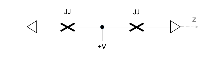
Figure 1: A quadrupole superconducting tunnelling junction device with minimum design. Note the two junctions are positioned on a line. The two ends of this line are grounded and the device is driven by an AC/DC voltage applied at the center.

Now, the averaged power of gravitational wave emission comes out as

$$P = \frac{G}{30c^{5}}\dddot{D}_{zz}^{\quad 2}\approx\left(\frac{Ge^{4}}{c^{5}\hbar^{6}}\right)5A_{z}^{4}M^{2}V^{4}K_{0}^{2},$$ (25)

where we have used the fact that the charge of the cooper pairs $q=2e$ is twice the charge of the electron. Interestingly, the smallness of the coupling constant $G/c^{5}$ is no longer an issue since $\hbar^{6}$ appears in the denominator, that is the coupling constant for this quantum process is given by

$$\frac{Ge^{4}}{c^{5}\hbar^{6}}\approx 6.5\times 10^{128}\quad{\rm C^{-3}s^{-5}V^{-7}}.$$ (26)

The structure of this newly emerged coupling constant reveals an interesting behaviour at the superconducting tunnelling junction, namely the dependence on the charge (electromagnetic energy) is stronger than the dependence on the mass. In other words, this set up channels electromagnetic energy into the geometric (gravitational) field with greater ease than simply converting mass into curvature (the classical einsteinean mechanism). We suppose that this is possible due to the quantum nature of the superconducting tunnelling junction.

The minimum design capable of producing a non-vanishing time dependent quadrupole mass moment is having two superconducting tunnelling junctions on a line (see Fig. 1). Such a device can be micro-fabricated and one possible such fabrication based on niobium metal ($T_{C}=9.26$ K) is depicted on Fig. 2.

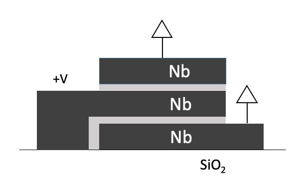
Figure 2: A quadrupole superconducting tunnelling junction device can be micro-fabricated on an insulating support by sequential evaporations of niobium metal. The insulating layers (thin light grey separations) essential for the operation of the tunnelling junction can be created by filling the vacuum chamber with oxygen after the niobium layer evaporation. Thus a natural layer of niobium oxide forms and has the sufficient thinness (few nm). The device is driven by the electrical scheme in Figure 1.

5 Conclusions

In consclusion, we would like to point out the main result of this paper - the charge density across a superconducting tunnelling junction changes with time, i.e. it is a rapidly oscillating function. The characteristic frequency of this oscillation is proportional to the coupling energy over Planck’s constant $\propto K_{0}/\hbar$. Since the cooper pairs are particles with a non-vanishing effective mass, at the superconducting tunnelling junction we have a condensed matter set up where rapid mass oscillations can arise. As a result, in a proper device (two superconducting junction on a line) electrical power (superconducting current times voltage) can be converted to gravitational wave emission. We believe, this compelling case can inspire an experimental verification attempt. Gravitation as a fundamental force has been explored only observationally. Here, we present an experimentally relevant situation in which gravitational waves can be artificially generated. This effectively opens the way to experimental exploration of gravitation.

Appendix

$$\dot{\phi} \approx \frac{qV}{\hbar}\quad\kappa={\rm const.}\quad\ddot{\phi}\approx\frac{q\dot{V}}{\hbar}$$ (27)

$$\dot{f} = -\frac{2K_{0}}{\hbar}\sin{\phi}$$ (28)

$$\ddot{f} = -\frac{2K_{0}}{\hbar}\cos{\phi}\dot{\phi}=-\frac{2qVK_{0}}{\hbar^{2}}\cos{\phi}$$ (29)

$$\dddot{f} = -\frac{2K_{0}}{\hbar}\cos{\phi}\ddot{\phi}+\frac{2K_{0}}{\hbar}\sin{\phi}(\dot{\phi})^{2}$$ (30)

$$=-\frac{2q\dot{V}K_{0}}{\hbar^{2}}\cos{\phi}+\frac{2q^{2}V^{2}K_{0}}{\hbar^{3}}\sin{\phi}$$

$$\approx\frac{2q^{2}V^{2}K_{0}}{\hbar^{3}}\sin{\phi}$$

References

- [1] R. P. Feynman, R. B. Leighton, and M. Sands, The Feynman lectures on physics, Addison‐Wesley, Reading, Mass, Vol. III, ch. 21 (1965).
- [2] K. K. Likharev, Dynamics of Josephson junctions and circuits, Gordon and Breach Sc. Publ. (1986).
- [3] Author’s personal correspondence with Physics Letters A regarding https://doi.org/10.1016/j.physleta.2019.126042 One referee wrote the following criticism of the idea that a quadrupole Josephson junction device can act as a gravitational wave emitter: ”My main problem with the proposed effect is the following: the current is a product of the electron density and their velocity (in the rest frame of ions). The Josephson current oscillations do not automatically imply mass oscillations - the density can remain constant, but the velocity can oscillate.”
- [4] H. B. Dwight, Tables of Integrals and other Mathematical Data., 4th Ed.,The Macmillan Co. New York and London, (1961).
- [5] L.D. Landau, E.M. Lifshitz, The Classical Theory of Fields, vol. 2, 3rd ed., Pergamon Press, ISBN 978-0-08-016019-1, (1971).
- [6] Victor Atanasov, Gravitational wave emission from quadrupole Josephson junction device, Phys. Lett. A 384, 126042 (2020).